We describe a new coordination activity and initial results for

a global synthesis of eddy covariance CH4 flux measurements.

FLUXNET-CH4 SYNTHESIS ACTIVITY

Objectives, Observations, and Future Directions

Sara H. Knox, robert b. JacKSon, benJamin Poulter, Gavin mcnicol, etienne Fluet-cHouinard, ZHen ZHanG, GuStaF HuGeliuS, PHiliPPe bouSquet, JoSeP G. canadell,

marielle SaunoiS, dario PaPale, HouSen cHu, trevor F. Keenan, denniS baldoccHi, marGaret S. torn, ivan mammarella, carlo trotta, miKa aurela, Gil boHrer,

david i. camPbell, aleSSandro ceScatti, Samuel cHamberlain, Jiquan cHen, Weinan cHen, SiGrid denGel, anKur r. deSai, euGenie euSKircHen, tHomaS FriborG, daniele GaSbarra, iGnacio Goded, matHiaS GoecKede, martin Heimann, manuel HelbiG, taKaSHi Hirano,

david Y. HollinGer, HiroKi iWata, minSeoK KanG, Janina Klatt, Ken W. KrauSS, larS KutZbacH, annalea loHila, bHaSKar mitra, timotHY H. morin, matS b. nilSSon, SHuli niu, aSKo noormetS,

Walter c. oecHel, mattHiaS PeicHl, olli Peltola, micHele l. reba, andreW d. ricHardSon, benJamin r. K. runKle, YounGrYel rYu, torSten SacHS, Karina v. r. ScHäFer, HanS Peter ScHmid, naraSinHa SHurPali, oliver SonnentaG, anGela c. i. tanG, maSaHito ueYama, rodriGo varGaS, timo veSala, eric J. Ward, liSamarie WindHam-mYerS, GeorG WoHlFaHrt, and donatella Zona

Atmospheric methane (CH4) is the second-most important anthropogenic greenhouse gas fol-lowing carbon dioxide (CO2) (Myhre et al. 2013).

The concentration of CH4 in the atmosphere today is about 2.5 times higher than in 1750 (Saunois et al. 2016a). The increase in atmospheric CH4 has arisen from human activities in agriculture, energy produc-tion, and waste disposal, and from changes in natural CH4 sources and sinks (Saunois et al. 2016a,b, 2017; Turner et al. 2019). Based on top-down atmospheric inversions, global CH4 emissions for the decade of 2003–12 were an estimated ~420 Tg C yr–1 (range 405–426 Tg C yr–1) (Saunois et al. 2016a). However, some analyses suggest that uncertainties in global CH4 sources and sinks are higher than those for CO2,

and uncertainties from natural sources exceed those from anthropogenic emissions (Saunois et al. 2016a). In particular, the largest source of uncertainty in the global CH4 budget is related to emissions from wetlands and inland waters (Saunois et al. 2016a; Melton et al. 2013; Bastviken et al. 2011). Wetland CH4 emissions may contribute as much as 25%–40% of the global total and are a leading source of interannual variability in total atmospheric CH4 concentrations (Bousquet et al. 2006; Chen and Prinn 2006; Saunois et al. 2016a).

Direct, ground-based measurements of in situ CH4 f luxes with high measurement frequency are important for understanding the responses of CH4 f luxes to environmental factors including climate,

2607AMERICAN METEOROLOGICAL SOCIETY |DECEMBER 2019Unauthenticated | Downloaded 01/03/22 02:04 PM UTC

AFFILIATIONS: Knox—Department of Earth System Science, Stanford University, Stanford, California, and Department of Geography, The University of British Columbia, Vancouver, British Columbia, Canada; JacKSon—Department of Earth System Science, Woods Institute for the Environment, and Precourt Institute for Energy, Stanford University, Stanford, California; Poulter—Bio-spheric Sciences Laboratory, NASA Goddard Space Flight Center, Greenbelt, Maryland; mcnicol and Fluet-cHouinard—Department of Earth System Science, Stanford University, Stanford, California; ZHanG—Department of Geographical Sciences, University of Mary-land, College Park, College Park, Maryland; HuGeliuS—Department of Physical Geography, and Bolin Centre for Climate Research, Stockholm University, Stockholm, Sweden; bouSquet and Sau-noiS—Laboratoire des Sciences du Climat et de l’Environnement, LSCE-IPSL, CEA-CNRS-UVSQ, Université Paris-Saclay, Gif-sur-Yvette, France; canadell—Global Carbon Project, Oceans and Atmosphere, CSIRO, Canberra, Australian Capital Territory, Australia; PaPale and trotta—Dipartimento per la Innovazione nei Sistemi Biologici, Agroalimentari e Forestali, Università degli Studi della Tuscia, Largo dell’Università, Viterbo, Italy; cHu, torn, and denGel—Earth and Environmental Sciences Area, Lawrence Berkeley National Lab, Berkeley, California; Keenan—Earth and Environmental Sciences Area, Lawrence Berkeley National Lab, and Department of Environmental Science, Policy and Management, University of California, Berkeley, Berkeley, California; baldoccHi and cHamberlain—Department of Environmental Science, Policy and Management, University of California, Berkeley, Berkeley, California; mammarella—Institute for Atmospheric and Earth System Research/Physics, Faculty of Science, University of Helsinki, Helsinki, Finland; aurela, loHila, and Peltola—Finnish Meteoro-logical Institute, Helsinki, Finland; boHrer—Department of Civil, Environmental and Geodetic Engineering, The Ohio State Univer-sity, Columbus, Ohio; camPbell—School of Science, University of Waikato, Hamilton, New Zealand; ceScatti and Goded—European Commission, Joint Research Centre (JRC), Ispra, Italy; J. cHen—Department of Geography, Environment, and Spatial Sciences, and Center for Global Change and Earth Observations, Michigan State, East Lansing, Michigan; W. cHen and niu—Key Laboratory of Eco-system Network Observation and Modeling, Institute of Geograph-ic Sciences and Natural Resources Research, Chinese Academy of Sciences, Beijing, China; deSai—Department of Atmospheric and Oceanic Sciences, University of Wisconsin–Madison, Madison, Wis-consin; euSKircHen—Institute of Arctic Biology, University of Alaska Fairbanks, Fairbanks, Alaska; FriborG—Department of Geosciences and Natural Resource Management, University of Copenhagen, Copenhagen, Denmark; GaSbarra—Department of Vegetal Biology, University of Napoli Federico II, and Institute for Mediterranean Agricultural and Forest Systems, CNR, Naples, Italy; GoecKede—Max Planck Institute for Biogeochemistry, Jena, Germany; Hei-mann—Max Planck Institute for Biogeochemistry, Jena, Germany, and Institute for Atmosphere and Earth System Research/Physics, Faculty of Science, University of Helsinki, Helsinki, Finland; HelbiG—School of Geography and Earth Sciences, McMaster University, Hamilton, Ontario, and Département de Géographie, Université de Montréal, Montreal, Quebec, Canada; Hirano—Research Faculty of Agriculture, Hokkaido University, Sapporo, Japan; HollinGer—Northern Research Station, Forest Service, USDA, Durham, New Hampshire; iWata—Department of Environmental Sciences, Shinshu

University, Matsumoto, Nagano, Japan; KanG—National Center for AgroMeteorology, Seoul, South Korea; Klatt—Institute of Meteo-rology and Climate Research, Karlsruhe Institute of Technology, Garmisch-Partenkirchen, Germany; KrauSS and Ward—Wetland and Aquatic Research Center, U.S. Geological Survey, Lafayette, Louisiana; KutZbacH—Institute of Soil Science, Center for Earth System Research and Sustainability, Universität Hamburg, Hamburg, Germany; mitra and noormetS—Department of Ecosystem Science and Management, Texas A&M University, College Station, Texas; morin—Department of Environmental Resources Engineering, State University of New York College of Environmental Science and Forestry, Syracuse, New York; nilSSon and PeicHl—Department of Forest Ecology and Management, Swedish University of Agricultural Sciences, Umeå, Sweden; oecHel—Department of Biology, San Diego State University, San Diego, California, and Department of Physical Geography, University of Exeter, Exeter, United Kingdom; reba—Delta Water Management Research Service, Agricultural Research Service, USDA, Jonesboro, Arkansas; ricHardSon—School of Informatics, Computing, and Cyber Systems, and Center for Ecosystem Science and Society, Northern Arizona University, Flagstaff, Arizona; runKle—Department of Biological and Agricul-tural Engineering, University of Arkansas, Fayetteville, Arkansas; rYu—Department of Landscape Architecture and Rural Systems Engineering, Seoul National University, Seoul, South Korea; SacHS—GFZ German Research Centre for Geoscience, Potsdam, Germany; ScHäFer—Department of Biological Sciences, Rutgers, The State University of New Jersey, Newark, New Jersey; ScHmid—Atmo-spheric Environmental Research, Institute of Meteorology and Climatology, Karlsruhe Institute of Technology, Garmisch-Parten-kirchen, Germany; SHurPali—Biogeochemistry Research Group, Department of Biological and Environmental Sciences, University of Eastern Finland, Kuopio, Finland; SonnentaG—Département de Géographie and Centre d’Études Nordiques, Université de Mon-tréal, Montreal, Quebec, Canada; tanG—Sarawak Tropical Peat Research Institute, Kota Samarahan, Sarawak, Malaysia; ueYama—Graduate School of Life and Environmental Sciences, Osaka Prefec-ture University, Sakai, Japan; varGaS—Department of Plant and Soil Sciences, University of Delaware, Newark, Delaware; veSala—Insti-tute for Atmospheric and Earth System Research/Physics, Faculty of Science, and Institute for Atmospheric and Earth System Research/Forest Sciences, Faculty of Agriculture and Forestry, University of Helsinki, Helsinki, Finland; WindHam-mYerS—Water Mission Area, U.S. Geological Survey, Menlo Park, California; WoHlFaHrt—De-partment of Ecology, University of Innsbruck, Innsbruck, Austria; Zona—Department of Biology, San Diego State University, San Diego, California, and Department of Animal and Plant Sciences, University of Sheffield, Sheffield, United KingdomCORRESPONDING AUTHOR: Sara Knox, saraknox.knox@gmail.com

The abstract for this article can be found in this issue, following the table of contents.DOI:10.1175/BAMS-D-18-0268.1

A supplement to this article is available online (10.1175/BAMS-D-18-0268.2)

In final form 11 June 2019©2019 American Meteorological SocietyFor information regarding reuse of this content and general copyright information, consult the AMS Copyright Policy.

2608 | DECEMBER 2019Unauthenticated | Downloaded 01/03/22 02:04 PM UTC

for providing validation datasets for the land surface models used to infer global CH4 budgets, and for constraining CH4 budgets. Eddy covariance (EC) flux towers measure real-time exchange of gases such as CO2, CH4, water vapor, and energy between the land surface and the atmosphere. The EC technique has emerged as a widespread means of measuring trace gas exchange because it provides direct and near-continuous ecosystem-scale flux measurements without disturbing the soil or vegetation (Baldocchi 2003; Aubinet et al. 2012). There are more than 900 reported active and historical flux tower sites globally and approximately 7,000 site years of data collected (Chu et al. 2017). While most of these sites measure CO2, water vapor, and energy exchange, the develop-ment of new and robust CH4 sensors has resulted in a rapidly growing number of CH4 EC measurements (Baldocchi 2014; Morin 2018), primarily in natural and agricultural wetlands (Petrescu et al. 2015).

Since the late 1990s, with a growing number of long-term, near-continuous EC measurements, the EC community has been well coordinated for inte-grating and synthesizing CO2, water vapor and energy fluxes. This cross-site coordination resulted in the development of regional f lux networks for Europe [EuroFlux, CarboEurope, and Integrated Carbon Observing System (ICOS)], Australia (OzFlux), North and South America (AmeriFlux, Large Biosphere Amazon, Fluxnet-Canada/Canadian Carbon Pro-gram, and MexFlux), Asia [AsiaFlux, ChinaFlux, Ko-Flux, and U.S.–China Carbon Consortium (USCCC)], and globally, FLUXNET (Papale et al. 2012; Baldoc-chi 2014). The resulting FLUXNET database (http://fluxnet.fluxdata.org/) has been used extensively to evaluate satellite measurements, inform Earth system models, generate data-driven CO2 flux products, and provide answers to a broad range of questions about atmospheric f luxes related to ecosystems, land use and climate (Pastorello et al. 2017). FLUXNET has grown steadily over the past 25 years, enhancing our understanding of carbon, water and energy cycles in terrestrial ecosystems (Chu et al. 2017).

Similar community efforts and syntheses for CH4 remain limited in part because EC measurements for CH4 fluxes were rarer until recently. Whereas the ear-liest EC measurements of CO2 fluxes date back to the late 1970s and early 1980s (Desjardins 1974; Anderson et al. 1984), the first EC CH4 flux measurements only began in the 1990s (Verma et al. 1992; Shurpali and Verma 1998; Fan et al. 1992; Kim et al. 1999), with reliable, easy-to-deploy field sensors only becom-ing available in the past decade or so. EC CH4 flux measurements became more feasible with advances

in sensor development, such as tunable diode laser absorption spectrometers, that allowed researchers to measure previously undetectable trace gas fluxes with higher signal to noise ratios (Rinne et al. 2007; McDermitt et al. 2011). After these new sensors were commercialized, and low-power, low-maintenance open-path sensors were developed that could be operated by solar panels in remote locations, the number of CH4 flux tower measurements increased substantially (Baldocchi 2014; Morin 2018). The rapidly growing number of EC CH4 flux measure-ments presents new opportunities for FLUXNET-type analyses and syntheses of ecosystem-scale CH4 flux observations.

This manuscript describes initial results from a new coordination activity for flux tower CH4 mea-surements organized by the Global Carbon Project (GCP) in collaboration with regional flux networks and FLUXNET. The goal of the activity is to develop a global database for EC CH4 observations to answer regional and global questions related to CH4 cycling. Here, we describe the objectives of the FLUXNET-CH4 activity, provide an overview of the current geographic and temporal coverage of CH4 flux mea-surements globally, present initial analyses exploring time scales of variability, uncertainty, trends, and drivers of CH4 f luxes across 60 sites, and discuss future research opportunities for examining controls on CH4 emissions and reducing uncertainties in the role of wetlands in the global CH4 cycle.

FLUXNET-CH4 SYNTHESIS OBJECTIVES AND TASKS. This activity is part of a larger GCP effort to establish and better constrain the global methane budget (www.globalcarbonproject.org /methanebudget/index.htm), and is designed to develop a CH4 database component in FLUXNET for a global synthesis of CH4 f lux tower data. To this end, we are surveying, assembling, and synthesiz-ing data from the EC community, in coordination with regional networks, including AmeriFlux’s 2019 “Year of Methane” (http://ameriflux.lbl.gov/year-of -methane/year-of-methane/), FLUXNET initiatives, and other complementary activities. In particular, this work is being carried out in parallel with the EU’s Readiness of ICOS for Necessities of Integrated Global Observations (RINGO) project, which is working to standardize protocols for f lux calcula-tions, quality control and gap-filling for CH4 f luxes (Nemitz et al. 2018). Methane-specific protocols are needed because of the added complexities and high variability of CH4 flux measurements and dynamics (Nemitz et al. 2018).

2609AMERICAN METEOROLOGICAL SOCIETY |DECEMBER 2019Unauthenticated | Downloaded 01/03/22 02:04 PM UTC

Our approach is to include all currently available and future CH4 flux tower observations in a global CH4 database, including freshwater, coastal, natural, and managed ecosystems, as well as upland ecosys-tems that may be measuring CH4 uptake by soils. The initiative is open to all members of the EC community. Database compilation began in 2017 and is ongoing. Data from sites in the Americas can be submitted to AmeriFlux (http://ameriflux.lbl.gov/data/how -to-uploaddownload-data/); otherwise, data can be submitted to the European Fluxes Database Cluster (www.europe-fluxdata.eu/home/sites-list).

In addition to many applications, an ultimate goal of the FLUXNET-CH4 activity is to generate a publicly available, open-access, data-driven global CH4 emis-sions product using similar machine-learning-based approaches used for CO2 f luxes (Jung et al. 2009; Tramontana et al. 2016). The product will be based on mechanistic factors associated with CH4 emissions and new spatiotemporal information on wetland area and dynamics for constraining CH4-producing areas. This gridded product will provide an independent bottom-up estimate of global wetland CH4 emissions to compare with estimates of global CH4 emissions from land surface models and atmospheric inversions. Recent work has shown the potential to upscale EC CH4 flux observations across northern wetlands, with predictive performance comparable to previous stud-ies upscaling net CO2 exchange (Peltola et al. 2019); however, our focus is on a globally gridded product.

The near-continuous, high-frequency nature of EC measurements also offers significant promise for improving our understanding of ecosystem-scale CH4 flux dynamics. As such, this synthesis also aims to investigate the dominant controls on net ecosystem-scale CH4 f luxes from hourly to interannual time scales across wetlands globally, and to characterize scale-emergent, nonlinear, and lagged processes of CH4 exchange.

Methane is produced during decomposition under anaerobic or reducing conditions and is transported to the atmosphere via plant-mediated transport, ebullition, and diffusion (Bridgham et al. 2013). During transport, CH4 can pass through un-saturated soil layers and be consumed or oxidized by aerobic bacteria (Wahlen 1993). Process-based biogeochemical models developed and applied at site, regional, and global scales simulate these indi-vidual processes with varying degrees of complexity (Bridgham et al. 2013; Melton et al. 2013; Poulter et al. 2017; Castro-Morales et al. 2018; Grant and Roulet 2002). The large range in predicted wetland CH4 emissions rates suggests that there is both

substantial parameter and structural uncertainty in large-scale CH4 flux models, even after account-ing for uncertainties in wetland areas (Poulter et al. 2017; Saunois et al. 2016a; Melton et al. 2013; Riley et al. 2011). A global EC CH4 database and associ-ated environmental variables can help constrain the parameterization of process-based biogeochemistry models (Saunois et al. 2016a; Bridgham et al. 2013; Oikawa et al. 2017). Furthermore, a key challenge is evaluating globally applicable process-based CH4 models at a spatial scale comparable to model grid cells (Melton et al. 2013; Riley et al. 2011). A globally gridded wetland CH4 emissions product upscaled from EC fluxes can help resolve this issue by provid-ing a scale-appropriate model evaluation dataset. As such, the global CH4 database and gridded product will also be used to parameterize and benchmark the performance of land surface models of global CH4 emissions, providing a unique opportunity for informing and validating biogeochemical models.

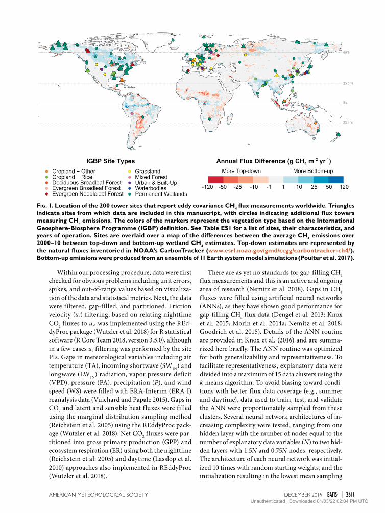
METHODS. Based on a survey of the EC com-munity (announced via the f luxnet-community @george.lbl.gov and AmeriFlux-Community@lbl.gov listservs), information available in regional networks and FLUXNET, and the scientific literature, we es-timate that at least 200 sites worldwide are currently applying the EC method for CH4 flux measurements (Fig. 1). Here we focus on findings from across 60 of the ~110 sites currently committed to participating in our FLUXNET-CH4 activity [Table A1 in the appen-dix and Table ES1 in the online supplemental material (https://doi.org/10.1175/BAMS-D-18-0268.2)]. Data from this initial set of sites were selected because they were publicly available or were contributed directly by site principal investigators (PIs). We will continue to engage the EC community more broadly and expand the database in the future.

Data standardization, gap-filling, and partitioning. We used similar data processing procedures as FLUXNET to standardize and gap-fill measurements, and in the case of net CO2 exchange, partition f luxes across sites (http://fluxnet.fluxdata.org/data/aboutdata/data -processing-101-pipeline-and-procedures/). Standard quality assurance and quality control of the data were first performed by site PIs. In nearly all cases, data collected by the local tower teams were first submit-ted to the data archives hosted by the regional flux networks, where data are prescreened and formatted based on the regional network data protocols. Data from the regional networks then entered our f lux processing procedure.

2610 | DECEMBER 2019Unauthenticated | Downloaded 01/03/22 02:04 PM UTC

Within our processing procedure, data were first checked for obvious problems including unit errors, spikes, and out-of-range values based on visualiza-tion of the data and statistical metrics. Next, the data were filtered, gap-filled, and partitioned. Friction velocity (u*) filtering, based on relating nighttime CO2 f luxes to u*, was implemented using the REd-dyProc package (Wutzler et al. 2018) for R statistical software (R Core Team 2018, version 3.5.0), although in a few cases u* filtering was performed by the site PIs. Gaps in meteorological variables including air temperature (TA), incoming shortwave (SWIN) and longwave (LWIN) radiation, vapor pressure deficit (VPD), pressure (PA), precipitation (P), and wind speed (WS) were filled with ERA-Interim (ERA-I) reanalysis data (Vuichard and Papale 2015). Gaps in CO2 and latent and sensible heat f luxes were filled using the marginal distribution sampling method (Reichstein et al. 2005) using the REddyProc pack-age (Wutzler et al. 2018). Net CO2 f luxes were par-titioned into gross primary production (GPP) and ecosystem respiration (ER) using both the nighttime (Reichstein et al. 2005) and daytime (Lasslop et al. 2010) approaches also implemented in REddyProc (Wutzler et al. 2018).

There are as yet no standards for gap-filling CH4 flux measurements and this is an active and ongoing area of research (Nemitz et al. 2018). Gaps in CH4 f luxes were filled using artificial neural networks (ANNs), as they have shown good performance for gap-filling CH4 flux data (Dengel et al. 2013; Knox et al. 2015; Morin et al. 2014a; Nemitz et al. 2018; Goodrich et al. 2015). Details of the ANN routine are provided in Knox et al. (2016) and are summa-rized here briefly. The ANN routine was optimized for both generalizability and representativeness. To facilitate representativeness, explanatory data were divided into a maximum of 15 data clusters using the k-means algorithm. To avoid biasing toward condi-tions with better f lux data coverage (e.g., summer and daytime), data used to train, test, and validate the ANN were proportionately sampled from these clusters. Several neural network architectures of in-creasing complexity were tested, ranging from one hidden layer with the number of nodes equal to the number of explanatory data variables (N) to two hid-den layers with 1.5N and 0.75N nodes, respectively. The architecture of each neural network was initial-ized 10 times with random starting weights, and the initialization resulting in the lowest mean sampling

Fig. 1. Location of the 200 tower sites that report eddy covariance CH4 flux measurements worldwide. Triangles indicate sites from which data are included in this manuscript, with circles indicating additional flux towers measuring CH4 emissions. The colors of the markers represent the vegetation type based on the International Geosphere-Biosphere Programme (IGBP) definition. See Table ES1 for a list of sites, their characteristics, and years of operation. Sites are overlaid over a map of the differences between the average CH4 emissions over 2000–10 between top-down and bottom-up wetland CH4 estimates. Top-down estimates are represented by the natural fluxes inventoried in NOAA’s CarbonTracker (www.esrl.noaa.gov/gmd/ccgg/carbontracker-ch4/). Bottom-up emissions were produced from an ensemble of 11 Earth system model simulations (Poulter et al. 2017).

2611AMERICAN METEOROLOGICAL SOCIETY |DECEMBER 2019Unauthenticated | Downloaded 01/03/22 02:04 PM UTC

error was selected. The simplest architecture, whereby additional increases in complexity resulted in <5% reduction in mean squared error, was chosen and the prediction saved. This procedure was repeated with 20 resamplings of the data, and missing half hours were filled using the median prediction. A standard set of variables available across all sites were used to gap-fill CH4 f luxes (Dengel et al. 2013), including TA, SWIN, WS, PA, and sine and cosine functions to represent seasonality. These meteorological variables were selected since they are relevant to CH4 exchange and were gap-filled using the ERA-I reanalysis data. Other variables related to CH4 exchange such as water table depth (WTD) or soil temperature (TS) were not included as explanatory variables as they were not available across all sites or had large gaps that could not be filled using the ERA-I reanalysis data. These missing data for variables highlight some of the key challenges in standardizing CH4 gap-filling methods across sites and emphasize the need for standardized protocols of auxiliary measurements across sites (cf. “Future research directions and needs” section) (Nemitz et al. 2018; Dengel et al. 2013). ANN gap-filling was performed using MATLAB (MathWorks 2018, version 9.4.0).

Annual CH4 budgets represent gap-filled, half-hourly fluxes integrated over an entire year or grow-ing season. If fluxes were only measured during the growing season, we assumed that fluxes outside of this period were negligible, although we acknowl-edge that cold season fluxes can account for as much as ~13%–50% of the annual CH4 emissions in some locations (Zona et al. 2016; Treat et al. 2018b; Helbig et al. 2017a; Kittler et al. 2017).

Uncertainty estimation. ANNs were also used to es-timate annual gap-filled and random uncertainty in CH4 flux measurements (Richardson et al. 2008; Moffat et al. 2007; Anderson et al. 2016; Knox et al. 2018). Here, we focus on assessing the random er-ror, but a full assessment of total flux measurement error also requires quantifying systematic error or bias (Baldocchi 2003). Systematic errors, due to incomplete spectral response, lack of nocturnal mix-ing, submesoscale circulations, and other factors are discussed elsewhere (Baldocchi 2003; Peltola et al. 2015) and are the focus of other ongoing initiatives.

Random errors in EC f luxes follow a double exponential (Laplace) distribution with a standard deviation varying with flux magnitude (Richardson et al. 2012, 2006). Model residuals of gap-filling algorithms such as ANNs provide a reliable, and conservative “upper limit,” estimate of the random

f lux uncertainty (Moffat et al. 2007; Richardson et al. 2008). For half-hourly CH4 flux measurements, random error was estimated using the residuals of the median ANN predictions. At each site, the probability density function (PDF) of the random f lux measurement error more closely followed a double-exponential (Laplace) rather than normal (Gaussian) distribution, with the root-mean-square error (RMSE) for the Laplace distribution fitted to the PDF of random errors consistently lower than the normal distributed error. From half-hourly flux measurements, random error can also be estimated using the daily differencing approach (Richard-son et al. 2012). Random error estimates [σ(δ)], as expressed as the standard deviation of the double-exponential distribution with scaling parameter β, where σ(δ) = √

–2β (Richardson et al. 2006), were

found to be nearly identical using the two approaches [σ(δ)model_residual = 1.0 × σ(δ)daily_differencing + 1.21; r2 = 0.97, p < 0.001], supporting the use of the model residual approach for estimating random error. As discussed below, σ(δ) scaled linearly with the magnitude of CH4 fluxes at nearly all sites. To quantify random uncer-tainty of cumulative fluxes, we used a Monte Carlo simulation that randomly draws 1,000 random errors for every original measurement using σ(δ) binned by flux magnitude, and then computed the variance of the cumulative sums (Anderson et al. 2016). For gap-filled values, the combined gap-filling and ran-dom uncertainty was calculated from the variance of the cumulative sums of the 20 ANN predictions (Anderson et al. 2016; Oikawa et al. 2017; Knox et al. 2015). The annual cumulative uncertainty at 95% confidence was estimated by adding the cumulative gap-filling and random measurement uncertain-ties in quadrature (Richardson and Hollinger 2007; Anderson et al. 2016). Note that when reporting mean or median annual CH4 fluxes across sites, error bars represent the standard error.

Wavelet-based time-scale decomposition. Methane fluxes are highly dynamic and vary across a range of time scales (Sturtevant et al. 2016; Koebsch et al. 2015). For example, in wetlands with permanent in-undation, the seasonal variation of CH4 exchange is predominantly controlled by temperature and plant phenology (Chu et al. 2014; Sturtevant et al. 2016). Ecosystem CH4 exchange also varies considerably at both longer (e.g., interannual; Knox et al. 2016; Rinne et al. 2018) and shorter (e.g., weeks, days, or hours; Koebsch et al. 2015; Hatala et al. 2012; Schaller et al. 2018) time scales. Wavelet decomposition is a particu-larly useful tool for investigating scale in geophysical

2612 | DECEMBER 2019Unauthenticated | Downloaded 01/03/22 02:04 PM UTC

and ecological analysis (Cazelles et al. 2008; Torrence and Compo 1998), because it can characterize both the time scale and location of patterns and pertur-bations in the data. Partitioning variability across temporal scales can help to isolate and characterize important processes (Schaller et al. 2018).

The maximal overlap discrete wavelet transform (MODWT) was used to decompose the time scales of variability in gap-filled CH4 flux measurements, as described in Sturtevant et al. (2016). The MODWT al-lows the time series to be decomposed into the detail added from progressively coarser to finer scales and either summed or treated individually to investigate patterns across scales. We reconstructed the detail in the fluxes for dyadic scales 1 (21 measurements = 1 h) to 14 (214 measurements = 341 days). Since patterns generated by ecological processes tend to occur over a scale range rather than at one individual scale, the detail over adjacent scales were summed to analyze four general time scales of variation (Sturtevant et al. 2016). These time scales included the “hourly” scale (1–2 h) representing perturbations such the passage of clouds overhead and turbulent scales up to the spectral gap, the “diel” scale (4 h to 1.3 days) encom-passing the diel cycles in sunlight and temperature, the “multiday” scale (2.7 to 21.3 days) ref lecting synoptic weather variability or fluctuations in water levels, and the “seasonal” scale (42.7 to 341 days) representing the annual solar cycle and phenology. Data were wavelet decomposed into the hourly, diel, and multiday scales using the Wavelet Methods for Time Series Analysis (WMTSA) Wavelet Toolkit in MATLAB.

Statistical analysis. We tested for significant relation-ships between log-transformed annual CH4 emissions and a number of covariates using linear mixed-effects models as described in Treat et al. (2018b). The pre-dictor variables of CH4 flux we evaluated included: biome or ecosystem type (categorical variables), and continuous biophysical variables including mean seasonal WTD, mean annual soil and air temperature (TMST and TMAT, respectively), net ecosystem exchange (NEE), GPP, and ER. When considering continuous variables, we focused on freshwater wetlands for comparison with previous CH4 synthesis activities. Soil temperature was measured between 2 and 25 cm below the surface in different studies. The results below are presented for GPP and ER covariates that are partitioned using the nighttime flux partitioning algorithm (Wutzler et al. 2018; Reichstein et al. 2005), although similar findings were obtained using daytime partitioned estimates. Additionally, individual sites or

site years were excluded when gaps in measurements exceeded two consecutive months, which explains the differences in the number of sites and site years in the “Environmental controls on annual CH4 emissions across freshwater wetland sites” section below.

Mixed-effects modeling was used because of the potential bias of having measurements over several years, with site included as a random effect in the analysis (Treat et al. 2018b). The significance of in-dividual predictor variables was evaluated using a χ2 test against a null model using only site as a random variable (Bates et al. 2015), with both models fit without reduced maximum likelihood. For multiple linear regression models, we used the model selection process outlined in Zuur et al. (2009). To incorporate annual cumulative uncertainty when assessing the significance of trends and differences in annual CH4 fluxes across biomes and ecosystem types, we used a Monte Carlo simulation that randomly draws 1,000 annual cumulative uncertainties for each estimate of annual CH4 flux. For each random draw the signifi-cance of the categorical variable was tested using a χ2 test against the null model with only site as a ran-dom variable. We report the marginal r2 (r2

m), which describes the proportion of variance explained by the fixed factors alone (Nakagawa and Schielzeth 2013). The mixed-effects modeling was implemented using the lmer command from the lme4 package (Bates et al. 2015) for R statistical software.

RESULTS AND DISCUSSION. Geographic and temporal coverage of eddy covariance CH4 flux measure-ments. We identified 200 sites worldwide that are applying the EC method for CH4 (Fig. 1; Table ES1); wetlands (including natural, managed, and restored wetlands) comprise the majority of sites (59%), with rice agriculture (10%) as the second-most represented vegetation type. The predominance of wetland and rice paddy sites in the database is unsurprising be-cause many studies are designed to target ecosystems expected to have relatively large CH4 emissions. However, there are also sites in ecosystems that are typically smaller sources or even sinks of CH4 such as upland forests (13%) and grasslands (8%). Additionally, six sites (~3%) are urban, with another five sites measuring CH4 f luxes from open water bodies. Although identified sites span all continents except Antarctica, the majority are concentrated in North America and Europe, with a growing number of sites in Asia (Fig. 1; Table ES1).

Measurements of CH4 fluxes cover a broad range of climates and a large fraction of wetland habitats (Fig. 2), with the tropics and tropical wetlands notably

2613AMERICAN METEOROLOGICAL SOCIETY |DECEMBER 2019Unauthenticated | Downloaded 01/03/22 02:04 PM UTC

underrepresented. As discussed below (see “Future research directions and needs” section), one impor-tant goal of FLUXNET and the regional networks is to increase site representativeness and extend mea-surements in undersampled regions. Increasing the number of tropical sites is particularly important for CH4 because more than half of global CH4 emissions are thought to come from this region (Saunois et al. 2016a; Dean et al. 2018). Furthermore, compared to northern wetlands, their biogeochemistry remains relatively poorly understood (Mitsch et al. 2009; Pan-gala et al. 2017). We expect the number of CH4 flux sites and their geographic and temporal coverage to continue to increase, as has occurred through time for CO2, water vapor, and energy flux measurements in FLUXNET (Pastorello et al. 2017; Chu et al. 2017).

Long-term CH4 flux time series are key to under-standing the causes of year-to-year variability and

trends in fluxes (Chu et al. 2017; Euskirchen et al. 2017; Pugh et al. 2018). The longest continuous record of CH4 flux measurements, from a fen in Finland (Rinne et al. 2018), is now ~14 years and ongoing (Table ES1). Three other sites have measurements exceeding 10 years; however, the median length is 5 years, with most sites established from 2013 onward (Table ES1). Longer time series are also important for both explor-ing the short- and long-term effects of extreme events on f luxes and tracking the response of disturbed or restored ecosystems over time (Pastorello et al. 2017). Furthermore, they can help address new and emerging science questions, such as quantifying CH4 feedbacks to climate with rising temperatures and as-sociated changes in ecosystem composition, structure and function (Helbig et al. 2017a,b; Dean et al. 2018), and the role of wetland emissions in atmospheric CH4 variability (McNorton et al. 2016; Poulter et al. 2017).

CH4 fluxes and trends across biomes and ecosystem types. Half-hourly and annual net CH4 f luxes for the 60 sites currently included in the database ex-hibited strong variability across sites (Figs. 3 and 4). Across the dataset, the mean half-hourly CH4 f lux was greater than the median f lux, indicating a positively skewed distribution with infrequent, large emissions (Fig. 3a), similar to findings from chamber-based syntheses (Olefeldt et al. 2013; Turetsky et al. 2014). Mean and median CH4 f luxes were smaller at higher latitudes and larger at lower latitudes (Fig. 3b), comparable again to trends in CH4 f luxes observed in predominantly chamber-based syntheses (Bartlett and Harriss 1993; Turetsky et al. 2014; Treat et al. 2018b).

The continuous nature of EC flux measurements is well suited for quantifying annual ecosystem-scale CH4 budgets, along with accumulated uncertainty (cf. “Gap-filling performance and uncertainty quantifica-tion” section). Annual estimates of net CH4 flux for each of the 60 sites in the flux tower database ranged from −0.2 ± 0.02 g C m–2 yr–1 for an upland forest site to 114.9 ± 13.4 g C m–2 yr–1 for an estuarine freshwater marsh (Rey-Sanchez et al. 2018), with fluxes exceeding 40 g C m–2 yr–1 at multiple sites (Fig. 4b). These emis-sions are of a considerably broader range and have much higher annual values than in an earlier synthesis by Baldocchi (2014), which included published values from 13 sites (Fig. 4a); median annual CH4 f luxes (±SE) in that study were 6.4 ± 1.9 g C m–2 yr–1, com-pared with 10.0 ± 1.6 g C m–2 yr–1 for our expanded database. Annual CH4 sums in our database were positively skewed, with skewness increasing with ad-ditional observations due largely to the inclusion of

Fig. 2. Distribution of sites by mean annual air temper-ature and precipitation. Tower locations are shown as circles or triangles (see Fig. 1), with vegetation type in color based on the IGBP definitions (CRO = croplands; DBF = deciduous broadleaf forests; EBF = evergreen broadleaf forests; ENF = evergreen needleleaf forests; GRA = grasslands; MF = mixed forests; URB = urban and built-up lands; WAT = water bodies; WET = per-manent wetlands). Gray dots represent annual mean temperature and total precipitation from the CRU TS 3.10 gridded climate dataset over the entire landmass (Harris et al. 2014), whereas blue dots represent grid cells with >25% wetland fraction as estimated using the Global Lakes and Wetlands Database (Lehner and Döll 2004). Temperature and precipitation grid cells included in this figure were averaged from 1981 to 2011, at 0.5° resolution.

2614 | DECEMBER 2019Unauthenticated | Downloaded 01/03/22 02:04 PM UTC

high CH4-emitting freshwater marsh sites (Fig. 4).

As suggested from Fig. 3b, annual wetland CH4 emissions differed significantly among biomes, even when consider-ing accumulated uncertainty [average Monte Carlo χ2 = 13.4 (12.1–14.7, 95% confidence interval), degrees of freedom (df) = 3, p < 0.05] (Table 1). Median CH4 emissions were significantly lower for tundra wetlands (2.9 ± 1.3 g C m–2 yr–1) than temperate wetlands (27.4 ± 3.4 g C m–2 yr–1). Higher CH4 emissions were observed from subtropical/tropical wetlands (43.2 ± 11.2 g C m–2 yr–1), based on only three site years of data; however, emphasizing the need for additional flux tower mea-surements in the tropics.

Whereas annual boreal/taiga wetland CH4 emis-sions were comparable to values reported in a recent synthesis of predominantly chamber-based CH4 flux measurements (Treat et al. 2018b), our tower-based measurements are ~50% lower and over 6 times higher for tundra and temperate wetlands, respec-tively (Table 1). The inconsistencies highlighted in Table 1 not only reflect the differences in the number and location of sites between datasets, but also the discrepancies resulting from different measurement

techniques. Several studies have noted consider-able differences in CH4 emissions measured using EC and chamber techniques, with estimates from chambers often higher than those from the EC mea-surements (Schrier-Uijl et al. 2010; Hendriks et al. 2010; Meijide et al. 2011; Krauss et al. 2016). This distinction highlights the need for additional studies investigating the systematic differences caused by the different spatial and temporal sampling footprints of these methods (Krauss et al. 2016; Morin et al. 2017;

Windham-Myers et al. 2018; Xu et al. 2017). Characterizing discrepancies between mea-surement techniques may also help constrain bottom-up estimates of CH4 emissions and reduce the disagreement of ~15 Tg C yr–1 between bot-tom-up (139 Tg CH4 yr–1) and top-down (125 Tg CH4 yr–1) es-timates of CH4 emissions from natural wetlands (Saunois et al. 2016a).

Annual CH4 emissions also differed significantly across ecosystems [average Monte Carlo χ2 = 45.5 (39.3–50.1), df = 9, p < 0.001; Fig. 5], with median f luxes highest for freshwater marshes (43.2 ±

Fig. 3. (a) Probability density function, and (b) cumulative frequency distri-bution of half-hourly CH4 flux (FCH4) data for sites currently included in the database (60 sites) aggregated by biome. Thin lines represent individual sites, whereas thicker lines present sites aggregated by biome. All cases are approximated by kernel density estimation. Note that whereas the x axis is scaled between −50 and 900 nmol m–2 s–1 for visualization purposes, some CH4 fluxes exceed this range.

Fig. 4. (a) Histogram of annual CH4 fluxes (FCH4; g C m–2 yr–1) measured with eddy covariance and published in the synthesis by Baldocchi (2014), and (b) histogram of our annual CH4 fluxes including additional site years of data estimated from the 60 sites listed in Table A1.

2615AMERICAN METEOROLOGICAL SOCIETY |DECEMBER 2019Unauthenticated | Downloaded 01/03/22 02:04 PM UTC

4.2 g C m–2 yr–1) and lowest for upland ecosystems (1.3 ± 0.7 g C m–2 yr–1). Treat et al. (2018b) also observed the highest annual emissions in marshes and re-ported a similar median value for temperate marshes (49.6 g C m–2 yr–1). Wet tundra and bogs had signifi-cantly lower annual emissions than marshes (Fig. 5), which in part reflects their presence in colder boreal and tundra systems, as well as differences in vegetation type, nutrient status, and hydrological regime (Treat et al. 2018b). Low median CH4 emission was observed from salt marshes in our dataset (0.8 ± 2.9 g C m–2 yr–1), because high sulfate concentrations inhibit methano-genesis (Poffenbarger et al. 2011; Holm et al. 2016). Even drained wetlands converted to agricultural land can be large sources of CH4 associated with seasonal flooding (Fig. 5). Median annual CH4 flux from rice was 12.6 ± 1.6 g C m–2 yr–1, which is slightly lower than the IPCC default value of 15 g C m–2 yr–1 (Sass 2003).

Environmental controls on annual CH4 emissions across freshwater wetland sites. Using an integrated CH4 flux database, we can begin to investigate the factors associated with varying CH4 emissions across sites. We explored the effects of WTD, TMST or TMAT, NEE, GPP, and ER on annual CH4 f lux. At global scales,

Table 1. Number of site years and characteristics of CH4 fluxes (g C m–2 yr–1) currently included in the data-base. Fluxes are compared with measurements reported in a recent synthesis of predominantly chamber-based CH4 flux measurements. Biome type was extracted from Olson et al. (2001) using site coordinates and includes tundra, boreal/taiga, temperate, and tropical/subtropical. Wetland CH4 emissions differed significantly across biomes, with letters indicating significant differences (α = 0.05) among biomes. Note that similar to our tower only dataset, values from Treat et al. (2018b) represent measured annual fluxes derived from a smaller dataset where measurements were made in the growing season and nongrowing season.

BiomeNo. of

site yearsMedian annual

CH4 flux25th

percentile75th

percentile References

Tundra

10 2.9 1.8 4.2 This study—All sites

10 2.9a 1.8 4.2 This study—Wetlands

31 5.6 1.0 11.4 Treat et al. (2018b)—All sites

26 6.3 3.0 16.4 Treat et al. (2018b)—Wetlands

Boreal and taiga

35 8.3 4.1 10.9 This study—All sites

30 9.5ab 6.0 11.3 This study—Wetlands

68 13.1 3.5 23.7 Treat et al. (2018b)—All sites

67 13.2 3.6 23.7 Treat et al. (2018b)—Wetlands

Temperate

72 16.4 7.9 35.9 This study—All sites

47 27.4b 10.0 47.3 This study—Wetlands

27 4.3 0.3 41.7 Treat et al. (2018b)—All sites

25 5.3 0.8 42.2 Treat et al. (2018b)—Wetlands

Tropical and subtropical

3 43.2 20.0 46.8 This study—All sites

3 43.2ab 20.0 46.8 This study—Wetlands

— — — — Treat et al. (2018b)—All sites

— — — — Treat et al. (2018b)—Wetlands

Fig. 5. Annual CH4 fluxes (FCH4; g C m–2 yr–1) among ecosystem types for the 60 sites currently included in the database (Table A1). Letters indicate significant differences (α = 0.05) among ecosystem types. Median value, first quartile, and third quartile are presented in the boxes, and dots represent outliers, which are defined as observations more than 1.5 times the inter-quartile range away from the top or bottom of the box.

2616 | DECEMBER 2019Unauthenticated | Downloaded 01/03/22 02:04 PM UTC

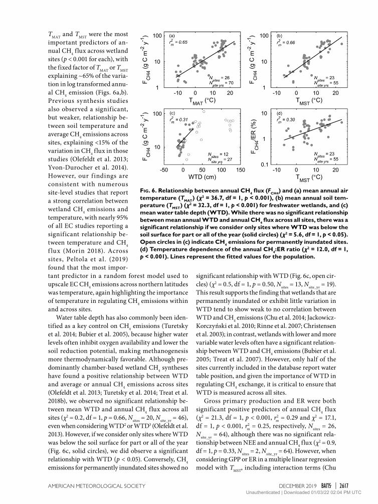
TMAT and TMST were the most important predictors of an-nual CH4 f lux across wetland sites (p < 0.001 for each), with the fixed factor of TMAT or TMST explaining ~65% of the varia-tion in log transformed annu-al CH4 emission (Figs. 6a,b). Previous synthesis studies also observed a significant, but weaker, relationship be-tween soil temperature and average CH4 emissions across sites, explaining <15% of the variation in CH4 flux in those studies (Olefeldt et al. 2013; Yvon-Durocher et al. 2014). However, our f indings are consistent with numerous site-level studies that report a strong correlation between wetland CH4 emissions and temperature, with nearly 95% of all EC studies reporting a significant relationship be-tween temperature and CH4 f lux (Morin 2018). Across sites, Peltola et a l . (2019) found that the most impor-tant predictor in a random forest model used to upscale EC CH4 emissions across northern latitudes was temperature, again highlighting the importance of temperature in regulating CH4 emissions within and across sites.

Water table depth has also commonly been iden-tified as a key control on CH4 emissions (Turetsky et al. 2014; Bubier et al. 2005), because higher water levels often inhibit oxygen availability and lower the soil reduction potential, making methanogenesis more thermodynamically favorable. Although pre-dominantly chamber-based wetland CH4 syntheses have found a positive relationship between WTD and average or annual CH4 emissions across sites (Olefeldt et al. 2013; Turetsky et al. 2014; Treat et al. 2018b), we observed no significant relationship be-tween mean WTD and annual CH4 f lux across all sites (χ2 = 0.2, df = 1, p = 0.66, Nsites = 20, Nsite_yr = 46), even when considering WTD2 or WTD3 (Olefeldt et al. 2013). However, if we consider only sites where WTD was below the soil surface for part or all of the year (Fig. 6c, solid circles), we did observe a significant relationship with WTD (p < 0.05). Conversely, CH4 emissions for permanently inundated sites showed no

significant relationship with WTD (Fig. 6c, open cir-cles) (χ2 = 0.5, df = 1, p = 0.50, Nsites = 13, Nsite_yr = 19). This result supports the finding that wetlands that are permanently inundated or exhibit little variation in WTD tend to show weak to no correlation between WTD and CH4 emissions (Chu et al. 2014; Jackowicz-Korczyński et al. 2010; Rinne et al. 2007; Christensen et al. 2003); in contrast, wetlands with lower and more variable water levels often have a significant relation-ship between WTD and CH4 emissions (Bubier et al. 2005; Treat et al. 2007). However, only half of the sites currently included in the database report water table position, and given the importance of WTD in regulating CH4 exchange, it is critical to ensure that WTD is measured across all sites.

Gross primary production and ER were both significant positive predictors of annual CH4 f lux (χ2 = 21.3, df = 1, p < 0.001, r2

m = 0.29 and χ2 = 17.1, df = 1, p < 0.001, r2

m = 0.25, respectively, Nsites = 26, Nsite_yr = 64), although there was no significant rela-tionship between NEE and annual CH4 flux (χ2 = 0.9, df = 1, p = 0.33, Nsites = 2, Nsite_yr = 64). However, when considering GPP or ER in a multiple linear regression model with TMST, including interaction terms (Chu

Fig. 6. Relationship between annual CH4 flux (FCH4) and (a) mean annual air temperature (TMAT) (χ2 = 36.7, df = 1, p < 0.001), (b) mean annual soil tem-perature (TMST) (χ2 = 32.3, df = 1, p < 0.001) for freshwater wetlands, and (c) mean water table depth (WTD). While there was no significant relationship between mean annual WTD and annual CH4 flux across all sites, there was a significant relationship if we consider only sites where WTD was below the soil surface for part or all of the year (solid circles) (χ2 = 5.6, df = 1, p < 0.05). Open circles in (c) indicate CH4 emissions for permanently inundated sites. (d) Temperature dependence of the annual CH4:ER ratio (χ2 = 12.0, df = 1, p < 0.001). Lines represent the fitted values for the population.

2617AMERICAN METEOROLOGICAL SOCIETY |DECEMBER 2019Unauthenticated | Downloaded 01/03/22 02:04 PM UTC

et al. 2014), neither GPP nor ER were significant, suggesting that the observed relationship with GPP or ER was due to covariation with soil temperature and, possibly, other environmental drivers.

The strong temperature dependence of ecosystem-scale CH4 emissions we observed across wetland sites is in line with the high temperature sensitivity of CH4 emissions found across microbial to ecosystem scales (Yvon-Durocher et al. 2014). CH4 emissions also have a higher temperature dependence than ER, such that the ratio of CH4 to CO2 emissions was found to increase markedly with seasonal increases in tem-perature (Yvon-Durocher et al. 2014). Similarly, we observed a significant increase in the ratio of annual CH4 to ER along geographic temperature gradients, ranging from 0.4% to 7.9%, with a median value of 2.8% across the dataset (Fig. 6d). This relationship suggests that warming may result in a greater relative contribution of CH4 to total carbon emissions from wetland ecosystems. With a growing FLUXNET CH4 database, it will be possible to further explore the dominant controls on CH4 f luxes within and across ecosystem types, as well as further investigate the temperature dependence of ecosystem-scale CH4 exchange (Schipper et al. 2014; Arcus et al. 2016; Yvon-Durocher et al. 2014).

Time scales of variability. Methane f luxes exhibited strong variability over a range of time scales, with the

variation across time scales differing between wetland types (Fig. 7). As observed previously (Sturtevant et al. 2016), the seasonal time scale dominated CH4 flux vari-ability across wetland types, but was most pronounced in rice paddies, which have a distinct growing season, and least pronounced in bogs (Fig. 7). Across ecosystem types, variation was lowest at the multiday scale, al-though multiday CH4 flux variation was slightly greater in rice paddies and wet tundra, potentially indicating greater water table fluctuations (Sturtevant et al. 2016), particularly at rice paddy sites, which are subject to seasonal drainage (Knox et al. 2016; Runkle et al. 2019). Whereas some studies report a strong diel pattern in CH4 emissions from wetlands and rice paddies (Knox et al. 2016; Chu et al. 2014; Morin et al. 2014b; Kim et al. 1999), others have found little or no diel variation (Rinne et al. 2018; Jackowicz-Korczyński et al. 2010; Yagi and Minami 1990; Nadeau et al. 2013). Across wetland types, diel variation was greatest in freshwater marshes (Fig. 7), which is consistent with the observa-tions that the vegetation at sites with a strong diel cycle of CH4 emissions is typically dominated by species with convective gas flow such as Phragmites australis or Typha spp. (Brix et al. 1992; Chanton et al. 1993). Bogs, fens, and wet tundra showed the greatest variation at the hourly scale (Fig. 7). This is likely in part due to typically lower fluxes at these sites as hourly pertur-bations of turbulent time series are largely dominated by noise (Hollinger and Richardson 2005), as well as the fact that near-surface turbulence and short-term pressure fluctuations can strongly influence CH4 ex-change in these peat dominated ecosystems (Nadeau et al. 2013; Sachs et al. 2008).

Gap-filling performance and uncertainty quantif ication. The performance of the neural networks varied strongly across sites (Fig. 8). Model r2, calculated from the median ANN prediction and observed f luxes at each site, ranged from ~0 to 0.92 across sites, with a median value of 0.41. Across sites, ANN performance was strongly linked to the percentage of total variance at diel and seasonal scales (r2 = 0.69, p < 0.001), indicating that across the wide range of observed flux magnitudes, sites with a more distinct seasonal and diel pattern tended to be more predict-able (Fig. 8). There was also a significant negative relationship between model r2 and the percentage of total variance at the hourly scale across sites (r2 = 0.72, p < 0.001), because, as noted previously, hourly per-turbations are largely dominated by noise (Hollinger and Richardson 2005).

Knowledge of the random errors in half-hourly f lux measurements is not only important for

Fig. 7. Variance of CH4 flux (FCH4) wavelet coefficients across time scales, as a percentage of the total variance, averaged by wetland type. Error bars represent the standard error. Note that only ecosystem types with at least 6 sites are shown here, including bogs, fens, freshwater (FW) marshes, rice paddies, and wet tundra.

2618 | DECEMBER 2019Unauthenticated | Downloaded 01/03/22 02:04 PM UTC

evaluating the uncertainty in cumulative fluxes (e.g., daily, monthly, or annual) and comparing f luxes across tower sites, but it also needed to incorporate information about random flux errors in model-data synthesis activities (Richardson et al. 2006). As noted above, random flux error more closely followed a Laplace rather than Gaussian distribution. Within sites, σ(δ) was not constant, but rather nearly always scaled with the magnitude of CH4 fluxes (Fig. 9a), as predicted from theory (Richardson et al. 2006). As observed for other fluxes (Richardson et al. 2006), both the slope and intercept of this relationship varied among sites, and depending on the sign of the flux (Fig. 9a). Across sites, random flux error therefore scaled linearly with the magnitude of mean CH4 flux (r2 = 0.86, p < 0.001), even when excluding the two highest CH4-emitting sites (r2 = 0.46, p < 0.001) (Fig. 9b). Whereas closed-path CH4 analyzers have been found to have lower random errors and instru-ment noise compared with open-path sensors (Peltola et al. 2014), there was no clear evidence of a systematic effect of the influence of closed- versus open-path sensors on random errors across sites (Fig. 9).

The total annual cumulative uncertainty in CH4 fluxes, including both random and gap-filling errors, ranged from ±0.01 to ±13.4 g C m–2 yr–1, with a me-dian value of ±1.0 g C m–2 yr–1 at 95% confidence (Fig. 10a). Relative error decreased expo-nentially with flux magnitude, ranging from 1.5% to 60% in most cases (Fig. 10b), although a few sites where annual CH4 sums were near zero had rela-tive errors exceeding 200% (data not shown). The high-est relative errors therefore tended to be associated with low CH4-emitting sites, such as upland sites and bogs, and the lowest relative errors were generally associated with high CH4-emitting sites such as freshwater marshes (Fig. 10b).

FUTURE RESEARCH D I R E C T I O N S A N D NEEDS. Better quantifica-tion of CH4 sources and sinks will improve estimates of re-gional and global CH4 budgets and reduce uncertainties in the CH4 cycle. In this general

Fig. 8. Relationship between the correlation coefficient (r2) calculated from the median ANN prediction and observed CH4 fluxes at each site and the percentage of total variance at diel and seasonal scales (r2 = 0.69, p < 0.001). Each site is color coded by ecosystem type. Sizes of the dots are proportional to the magnitude of mean CH4 flux, where flux magnitude was aggregated into 10 bins for plotting.

Fig. 9. (a) Scaling of FCH4 random flux measurement error [σ(δ)] with flux magnitude for all sites with a significant linear relationship between random error and flux magnitude (95% of all sites). Data at each site were placed into 10 bins (Oikawa et al. 2017). (b) Scaling of FCH4 random flux measurement error, characterized by the standard deviation of the double-exponential distribution [σ(δ)], with mean flux magnitude across sites. There was a significant linear relationship between σ(δ) and the magnitude of mean CH4 flux [σ(δ) = 0.5 × FCH4 + 5.9, r2 = 0.86, p < 0.001], even when excluding the two highest CH4-emitting sites [σ(δ) = 0.4 × FCH4 + 11.3, r2 = 0.46, p < 0.001]. Note that circles represent sites with open-path CH4 analyzers while asterisks represent sites with closed-path sensors.

2619AMERICAN METEOROLOGICAL SOCIETY |DECEMBER 2019Unauthenticated | Downloaded 01/03/22 02:04 PM UTC

context, high-frequency ob-servations of ecosystem-scale CH4 emissions should help constrain bottom-up CH4 budgets, improve our under-standing of the environmental factors controlling CH4 fluxes, and inform and validate land surface models used to esti-mate global CH4 f luxes. Un-like well-established efforts synthesizing CO2, water vapor, and energy observations, no such global data synthesis or initiative previously existed for CH4. The database pre-sented here addresses this gap with the EC community by organizing the collection and aggregation of a global EC CH4 database through FLUXNET.

EC flux data quality assessment. Much of what has been learned within FLUXNET for CO2, water vapor, and energy measurements is informing, and should continue to inform, new efforts for CH4. Reliable EC measure-ments of CO2 and water vapor f luxes have been conducted at hundreds of sites across broad regional networks (Papale et al. 2012), and substantial efforts have focused on developing best practices and har-monizing approaches across sites to ensure consistent, high-quality flux measurements (Aubinet et al. 1999; Reichstein et al. 2005; Moffat et al. 2007). CH4 fluxes are often characterized by small fluxes with episodic spikes, and additional research is needed to ensure reliable measurements (Peltola et al. 2014, 2013), and refine and standardize methods and routines for data processing and quality checking (Nemitz et al. 2018; Schaller et al. 2018). Recent efforts provided guidance on instrument selection, setup and maintenance, and data processing for EC CH4 flux measurements (Nemitz et al. 2018). However, with respect to instru-ment setup and data processing, more research is needed in best practices for storage flux quantifica-tion, despiking, and u* filtering (Nemitz et al. 2018).

Gap-f illing. Whereas neural networks have shown strong performance for gap-filling CH4 fluxes (Den-gel et al. 2013; Knox et al. 2016), our results reveal some of the challenges of gap-filling CH4 fluxes at sites with low fluxes and/or a lack of seasonal and diel variation (Fig. 8). More research is therefore needed

for best practices for gap-filling to estimate annual CH4 budgets (Nemitz et al. 2018). For example, there has yet to be a comprehensive analysis comparing a wide range of gap-filling approaches for CH4 fluxes similar to the study by Moffat et al. (2007) for CO2 exchange. While ANNs are one gap-filling method (Dengel et al. 2013; Shoemaker et al. 2014; Morin et al. 2014a), numerous other gap-filling approaches exist, including nonlinear regression techniques, mean diurnal variation, lookup tables, marginal distribu-tion sampling, and the multiple imputation method (Moffat et al. 2007; Vitale et al. 2019). Future efforts should focus on systematically investigating these approaches across a range of sites to provide best practices for gap-filling CH4 exchange.

Ancillary measurements. Along with research that addresses the challenges of measuring and process-ing EC CH4 f luxes, key ancillary variables to help gap-fill, predict, and scale CH4 f luxes should also be measured more comprehensively across sites. For instance, although WTD is known to strongly influence CH4 emissions (Turetsky et al. 2014; Treat et al. 2018b), as noted above, only half of the sites currently included in the database report water table position. Generally, EC CH4 measurements are implemented at sites also collecting CO2 f luxes and common meteorological measurements used in the f lux community; however, guidelines are only

Fig. 10. (a) Histogram of total random error (g C m–2 yr–1) in annual CH4 flux at 95% confidence, where count refers to the number of site years of measurements. The cumulative gap-filling and random measurement uncertainties of gap-filled and original values were added in quadrature to estimate the total random uncertainty at each site. (b) Relationship be-tween annual CH4 flux (g C m–2 yr–1) and relative error (i.e., total random error divided by flux magnitude; %).

2620 | DECEMBER 2019Unauthenticated | Downloaded 01/03/22 02:04 PM UTC

beginning to emerge for which additional support-ing variables should be collected at sites measuring CH4 f luxes (Nemitz et al. 2018).

Measurements of variables beyond those relevant for CO2 are needed to better understand and pre-dict the complex and interacting processes of CH4 production, consumption, and transport, the latter of which includes diffusion, ebullition, and plant-mediated transport. Guidance on the description of some basic variables affecting these processes is avail-able through new protocols in the flux community detailing soil meteorological measurements, ancillary vegetation measurements, and site description, man-agement and disturbance (Saunders et al. 2018; Op De Beeck et al. 2018; Gielen et al. 2018). These protocols provide guidance on variables such as soil tempera-ture and soil moisture profiles, water table depth and snow depth, soil pH and soil type, bulk density, and livestock density. However, although WTD is an eas-ily measured proxy for anaerobic conditions, direct and continuous measurement of redox potential and oxygen content in particular would be valu-able additional measurements (Nemitz et al. 2018). Similarly, measuring variables such as conductivity, below-ground CH4 concentrations, dissolved organic carbon concentrations, and the presence of alternative electron acceptors such as nitrate, iron, sulfate, and humic substances in the water and soil column would provide useful information for the interpretation of CH4 emissions. Stable isotope analyses of CH4 are also valuable as they provide important information on mechanisms of CH4 production, transport, and oxidation (Chanton et al. 1997; Marushchak et al. 2016). Detailed information on soil microbial com-munities driving CH4 production and consumption could also be helpful (Kwon et al. 2017). Vegetation biomass, species composition, and phenology are also important variables to consider, because plants are a primary source of carbon substrates for methano-genic metabolism, and they mediate CH4 transport through aerenchymous tissue (Kwon et al. 2017; Joabsson et al. 1999; Carmichael et al. 2014). New guidance is now available for such measurements at flux tower locations (Gielen et al. 2018; Hufkens et al. 2018). Continuing to develop a consensus on best practices for ancillary measurements is important for interpreting, gap-filling, and upscaling CH4 flux measurements.

Characterizing spatial variability. CH4 f luxes exhibit finescale spatial variability that can span orders of magnitude within a landscape (Peltola et al. 2015; Marushchak et al. 2016; Desai et al. 2015; Treat et al.

2018a; Iwata et al. 2018), attributable to heterogeneous soil properties and moisture conditions, vegetation composition, and land use (Davidson et al. 2016; Parmentier et al. 2011; Chamberlain et al. 2018). Furthermore, there is evidence that traditionally unmeasured surfaces (i.e., tree stems) are important sources of CH4 to the atmosphere and could explain spatial heterogeneity within ecosystems (Barba et al. 2019). Accurately representing spatial heterogeneity and the relative fraction of uplands and wetlands is imperative for interpreting and predicting CH4 emissions within many ecosystems, and for upscal-ing f lux measurements regionally and globally as wetlands are hot spots for carbon cycling (Treat et al. 2018a; Tuovinen et al. 2019; Rößger et al. 2019). Flux footprint analysis characterizing the fractional coverage of the dominant surface types, particu-larly the fraction of open water and aerenchymatous plants, is important for interpreting EC CH4 f lux measurements and quantifying annual CH4 budgets at spatially heterogeneous sites (Franz et al. 2016; Helbig et al. 2017a; Jammet et al. 2017) (Fig. 11). This integration can be achieved by combining CH4 mea-surements, flux footprint analysis, and near-surface

Fig. 11. Footprint climatology for a eutrophic shallow lake on a formerly drained fen in Germany (Zarnekow; DE-Zrk) illustrating the importance of footprint analy-sis for the interpretation of EC measurements of CH4. Here we used two footprint models, including the model of Kormann and Meixner (2001) (yellow) and Kljun et al. (2015) (white). The footprint climatology was calculated by aggregating all half-hour footprints within a year. The dashed lines enclose the areas aggre-gating to 80% of source areas, while solid lines enclose the 50% of source areas.

2621AMERICAN METEOROLOGICAL SOCIETY |DECEMBER 2019Unauthenticated | Downloaded 01/03/22 02:04 PM UTC

Table A1. The ecosystem type is based on the classification of Olefeldt et al. (2013) and Treat et al. (2018b). Biome was based on the classification of Olson et al. (2001) and extracted using site coordinates. Vegetation type was based on the International Geosphere-Biosphere Programme (IGBP) definition. Salinity regime includes freshwater (FW) or saltwater (SW) wetlands. Disturbance is based on the classification of Turetsky et al. (2014). Data from all sites are publicly available, primarily through AmeriFlux and the European Database Cluster, and in a few cases, through other databases/repositories. Site DOIs are specified where applicable.

Site ID Site name CountryLat (°N)

Lon (°E) Biome IGBP Ecosystem type Salinity

Wetland disturbance Site PI Data DOI/location

US-ICs Wet sedge tundra U.S. 68.606 −149.311 Tundra WET Wet tundra FW Undisturbed Eugenie Euskirchen DOI:10.17190/AMF/1246130SE-St1 Stordalen grassland (mire) Sweden 68.350 19.050 Tundra WET Fen FW Undisturbed Thomas Friborg European Fluxes Database ClusterSE-Sto Stordalen Palsa bog Sweden 68.356 19.050 Tundra WET Bog FW Undisturbed Thomas Friborg European Fluxes Database ClusterRU-Vrk Seida/Vorkuta Russia 67.055 62.940 Tundra WET Wet tundra FW Undisturbed Thomas Friborg European Fluxes Database ClusterRU-Ch2 Chersky reference Russia 68.617 161.351 Tundra WET Wet tundra FW Undisturbed Mathias Goeckede European Fluxes Database ClusterRU-Che Chersky Russia 68.613 161.341 Tundra WET Wet tundra FW Drying Mathias Goeckede European Fluxes Database ClusterRU-SAM Samoylov Russia 72.374 126.496 Tundra WET Wet tundra FW Undisturbed Torsten Sachs European Fluxes Database ClusterUS-NGB NGEE Barrow U.S. 71.280 −156.609 Tundra WET Wet tundra FW Undisturbed Margaret Torn DOI:10.17190/AMF/1436326US-Beo Barrow U.S. 71.281 −156.612 Tundra WET Wet tundra FW Undisturbed Donatella Zona AmeriFluxUS-Bes Barrow U.S. 71.281 −156.596 Tundra WET Wet tundra FW Undisturbed Donatella Zona AmeriFluxUS-Atq Atqasuk U.S. 70.470 −157.409 Tundra WET Wet tundra FW Undisturbed Donatella Zona DOI:10.17190/AMF/1246029US-Ivo Ivotuk U.S. 68.486 −155.750 Tundra WET Wet tundra FW Undisturbed Donatella Zona DOI:10.17190/AMF/1246067

— Black spruce forest U.S. 64.700 −148.320 Boreal forests/taiga ENF Upland — — Eugenie Euskirchen www.lter.uaf.edu/data/data-detail/id/708— Rich fen U.S. 64.704 −148.313 Boreal forests/taiga WET Fen FW Undisturbed Eugenie Euskirchen www.lter.uaf.edu/data/data-detail/id/708— Thermokarst collapse scar bog U.S. 64.700 −148.320 Boreal forests/taiga WET Bog FW Undisturbed Eugenie Euskirchen www.lter.uaf.edu/data/data-detail/id/708

FI-Lom Lompolojankka Finland 67.997 24.209 Boreal forests/taiga WET Fen FW Undisturbed Annalea Lohila European Fluxes Database ClusterSE-Deg Degero Sweden 64.182 19.557 Boreal forests/taiga WET Fen FW Undisturbed Matthias Peichl, Mats Nilsson European Fluxes Database ClusterCA-SCC Scotty Creek—Peat plateau/collapse scar Canada 61.308 −121.299 Boreal forests/taiga ENF Peat plateau FW — Oliver Sonnentag DOI:10.17190/AMF/1480303CA-SCB Scotty Creek bog Canada 61.309 −121.299 Boreal forests/taiga WET Bog FW Undisturbed Oliver Sonnentag AmeriFluxUS-NGC NGEE Arctic Council U.S. 64.861 −163.701 Boreal forests/taiga WET Wet tundra FW Undisturbed Margaret Torn AmeriFluxUS-Uaf University of Alaska Fairbanks U.S. 64.866 −147.856 Boreal forests/taiga WET Bog FW Undisturbed Masahito Ueyama DOI:10.17190/AMF/1480322FI-Sii Siikaneva I (FI-Sii) Finland 61.833 24.193 Boreal forests/taiga WET Fen FW Undisturbed Timo Vesala, Ivan Mammarella European Fluxes Database ClusterFI-Si2 Siikaneva II Finland 61.837 24.170 Boreal forests/taiga WET Bog FW Undisturbed Timo Vesala, Ivan Mammarella European Fluxes Database ClusterUS-Myb Mayberry wetland U.S. 38.050 −121.765 Temperate WET Marsh FW Wetting Dennis Baldocchi DOI:10.17190/AMF/1246139US-Sne Sherman Island restored wetland U.S. 38.037 −121.755 Temperate WET Marsh FW Wetting Dennis Baldocchi DOI:10.17190/AMF/1418684US-Tw1 Twitchell west pond wetland U.S. 38.107 −121.647 Temperate WET Marsh FW Wetting Dennis Baldocchi DOI:10.17190/AMF/1246147US-Tw4 Twitchell east end wetland U.S. 38.103 −121.641 Temperate WET Marsh FW Wetting Dennis Baldocchi DOI:10.17190/AMF/1246148US-Twt Twitchell rice U.S. 38.109 −121.653 Temperate CRO - Rice Rice FW — Dennis Baldocchi DOI:10.17190/AMF/1246151US-Bi2 Bouldin Island corn U.S. 38.109 −121.535 Temperate CRO - Other Drained/agricultural wetland FW Drying Dennis Baldocchi DOI:10.17190/AMF/1419513US-Bi1 Bouldin Island alfalfa U.S. 38.102 −121.504 Temperate CRO - Other Drained/agricultural wetland FW Drying Dennis Baldocchi DOI:10.17190/AMF/1480317US-Snd Sherman Island U.S. 38.037 −121.754 Temperate CRO - Other Drained/agricultural wetland FW Drying Dennis Baldocchi DOI:10.17190/AMF/1246094US-OWC Old Woman Creek U.S. 41.380 −82.512 Temperate WET Marsh FW Undisturbed Gil Bohrer DOI:10.17190/AMF/1246094US-Orv Olentangy River Wetland Research Park U.S. 40.020 −83.018 Temperate WET Marsh FW Undisturbed Gil Bohrer DOI:10.17190/AMF/1246135NZ-Kop Kopuatai New Zealand −37.388 175.554 Temperate WET Bog FW Undisturbed Dave Campbell https://researchcommons.waikato.ac.nz/handle/10289/11393IT-Cas Castellaro Italy 45.070 8.718 Temperate CRO - Rice Rice FW — Alessandro Cescatti European Fluxes Database ClusterUS-WPT Winous Point north marsh U.S. 41.465 −82.996 Temperate WET Marsh FW Wetting Jiquan Chen, Housen Chu DOI:10.17190/AMF/1246155US-CRT Curtice Walter-Berger cropland U.S. 41.628 −83.347 Temperate CRO - Other Upland — — Jiquan Chen, Housen Chu DOI:10.17190/AMF/1246156US-Los Lost Creek U.S. 46.083 −89.979 Temperate WET Fen FW Undisturbed Ankur Desai DOI:10.17190/AMF/1246071JP-Mse Mase paddy flux site (MSE) Japan 36.054 140.027 Temperate CRO - Rice Rice FW — Akira Miyata European Fluxes Database ClusterJP-Swl Suwa Lake site Japan 36.047 138.108 Temperate WAT Waterbody FW Undisturbed Hiroki Iwata European Fluxes Database ClusterIT-BCi Borgo Cioffi Italy 40.524 14.957 Temperate CRO - Other Upland — — Vincenzo Magliulo European Fluxes Database Cluster

— Hongyuan China 32.800 102.550 Temperate GRA Upland — — Shuli Niu European Fluxes Database ClusterUS-NC4 NC Alligator River U.S. 35.788 −75.904 Temperate WET Swamp FW Undisturbed Asko Noormets DOI:10.17190/AMF/1480314DE-SfN Schechenfilz Nord Germany 47.806 11.328 Temperate WET Bog FW Undisturbed Hans Peter Schmid European Fluxes Database ClusterUS-Ho1 Howland Forest (main tower) U.S. 45.204 −68.740 Temperate ENF Upland — — Andrew Richardson DOI:10.17190/AMF/1246061US-HRA Humnoke farm rice field AWD, United States U.S. 34.585 −91.752 Temperate CRO - Rice Rice FW — Benjamin Runkle AmeriFluxUS-HRC Humnoke farm rice field conventional, United States U.S. 34.589 −91.752 Temperate CRO - Rice Rice FW — Benjamin Runkle AmeriFluxKR-CRK Cheorwon rice paddy South Korea 38.201 127.251 Temperate CRO - Rice Rice FW — Youngryel Ryu, Minseok Kang European Fluxes Database ClusterDE-Zrk Zarnekow Germany 53.876 12.889 Temperate WET Fen FW Wetting Torsten Sachs European Fluxes Database ClusterDE-Dgw Dagowsee Germany 53.151 13.054 Temperate WAT Waterbody FW Undisturbed Torsten Sachs European Fluxes Database ClusterUS-MRM Marsh Resource Meadowlands Mitigation Bank U.S. 40.816 −74.044 Temperate WET Salt marsh SW Wetting Karina Schäfer AmeriFlux

— Bog Lake peatland U.S. 47.530 −93.470 Temperate WET Fen FW Undisturbed Shahi Verma AmeriFlux— MacArthur Agro-Ecology Research Center U.S. 27.163 −81.187 Temperate CRO - Other Drained/agricultural wetland FW Drying Jed Sparks, Samuel Chamberlain AmeriFlux

JP-BBY Bibai bog Japan 43.323 141.811 Temperate WET Bog FW Undisturbed Masahito Ueyama European Fluxes Database ClusterUS-StJ St. Jones Reserve U.S. 39.088 −75.437 Temperate WET Salt marsh SW Undisturbed Rodrigo Vargas DOI:10.17190/AMF/1480316US-Srr Suisun marsh—Rush Ranch U.S. 38.201 −122.026 Temperate WET Salt marsh SW Undisturbed Lisamarie Windham-Myers DOI:10.17190/AMF/1418685AT-Neu Neustift Austria 47.117 11.318 Temperate GRA Upland — — Georg Wohlfahrt European Fluxes Database ClusterUS-LA2 Salvador WMA freshwater marsh U.S. 29.859 −90.287 Tropical and subtropical WET Marsh FW Undisturbed Ken Krauss AmeriFluxUS-LA1 Pointe-aux-Chenes brackish marsh U.S. 29.501 −90.445 Tropical and subtropical WET Salt marsh SW Undisturbed Ken Krauss AmeriFluxMY-MLM Maludam Malaysia 1.454 111.149 Tropical and subtropical WET Swamp FW Undisturbed Angela Tang DOI:10.5281/zenodo.1161966

2622 | DECEMBER 2019Unauthenticated | Downloaded 01/03/22 02:04 PM UTC

Table A1. The ecosystem type is based on the classification of Olefeldt et al. (2013) and Treat et al. (2018b). Biome was based on the classification of Olson et al. (2001) and extracted using site coordinates. Vegetation type was based on the International Geosphere-Biosphere Programme (IGBP) definition. Salinity regime includes freshwater (FW) or saltwater (SW) wetlands. Disturbance is based on the classification of Turetsky et al. (2014). Data from all sites are publicly available, primarily through AmeriFlux and the European Database Cluster, and in a few cases, through other databases/repositories. Site DOIs are specified where applicable.

Site ID Site name CountryLat (°N)

Lon (°E) Biome IGBP Ecosystem type Salinity

Wetland disturbance Site PI Data DOI/location

US-ICs Wet sedge tundra U.S. 68.606 −149.311 Tundra WET Wet tundra FW Undisturbed Eugenie Euskirchen DOI:10.17190/AMF/1246130SE-St1 Stordalen grassland (mire) Sweden 68.350 19.050 Tundra WET Fen FW Undisturbed Thomas Friborg European Fluxes Database ClusterSE-Sto Stordalen Palsa bog Sweden 68.356 19.050 Tundra WET Bog FW Undisturbed Thomas Friborg European Fluxes Database ClusterRU-Vrk Seida/Vorkuta Russia 67.055 62.940 Tundra WET Wet tundra FW Undisturbed Thomas Friborg European Fluxes Database ClusterRU-Ch2 Chersky reference Russia 68.617 161.351 Tundra WET Wet tundra FW Undisturbed Mathias Goeckede European Fluxes Database ClusterRU-Che Chersky Russia 68.613 161.341 Tundra WET Wet tundra FW Drying Mathias Goeckede European Fluxes Database ClusterRU-SAM Samoylov Russia 72.374 126.496 Tundra WET Wet tundra FW Undisturbed Torsten Sachs European Fluxes Database ClusterUS-NGB NGEE Barrow U.S. 71.280 −156.609 Tundra WET Wet tundra FW Undisturbed Margaret Torn DOI:10.17190/AMF/1436326US-Beo Barrow U.S. 71.281 −156.612 Tundra WET Wet tundra FW Undisturbed Donatella Zona AmeriFluxUS-Bes Barrow U.S. 71.281 −156.596 Tundra WET Wet tundra FW Undisturbed Donatella Zona AmeriFluxUS-Atq Atqasuk U.S. 70.470 −157.409 Tundra WET Wet tundra FW Undisturbed Donatella Zona DOI:10.17190/AMF/1246029US-Ivo Ivotuk U.S. 68.486 −155.750 Tundra WET Wet tundra FW Undisturbed Donatella Zona DOI:10.17190/AMF/1246067

— Black spruce forest U.S. 64.700 −148.320 Boreal forests/taiga ENF Upland — — Eugenie Euskirchen www.lter.uaf.edu/data/data-detail/id/708— Rich fen U.S. 64.704 −148.313 Boreal forests/taiga WET Fen FW Undisturbed Eugenie Euskirchen www.lter.uaf.edu/data/data-detail/id/708— Thermokarst collapse scar bog U.S. 64.700 −148.320 Boreal forests/taiga WET Bog FW Undisturbed Eugenie Euskirchen www.lter.uaf.edu/data/data-detail/id/708

FI-Lom Lompolojankka Finland 67.997 24.209 Boreal forests/taiga WET Fen FW Undisturbed Annalea Lohila European Fluxes Database ClusterSE-Deg Degero Sweden 64.182 19.557 Boreal forests/taiga WET Fen FW Undisturbed Matthias Peichl, Mats Nilsson European Fluxes Database ClusterCA-SCC Scotty Creek—Peat plateau/collapse scar Canada 61.308 −121.299 Boreal forests/taiga ENF Peat plateau FW — Oliver Sonnentag DOI:10.17190/AMF/1480303CA-SCB Scotty Creek bog Canada 61.309 −121.299 Boreal forests/taiga WET Bog FW Undisturbed Oliver Sonnentag AmeriFluxUS-NGC NGEE Arctic Council U.S. 64.861 −163.701 Boreal forests/taiga WET Wet tundra FW Undisturbed Margaret Torn AmeriFluxUS-Uaf University of Alaska Fairbanks U.S. 64.866 −147.856 Boreal forests/taiga WET Bog FW Undisturbed Masahito Ueyama DOI:10.17190/AMF/1480322FI-Sii Siikaneva I (FI-Sii) Finland 61.833 24.193 Boreal forests/taiga WET Fen FW Undisturbed Timo Vesala, Ivan Mammarella European Fluxes Database ClusterFI-Si2 Siikaneva II Finland 61.837 24.170 Boreal forests/taiga WET Bog FW Undisturbed Timo Vesala, Ivan Mammarella European Fluxes Database ClusterUS-Myb Mayberry wetland U.S. 38.050 −121.765 Temperate WET Marsh FW Wetting Dennis Baldocchi DOI:10.17190/AMF/1246139US-Sne Sherman Island restored wetland U.S. 38.037 −121.755 Temperate WET Marsh FW Wetting Dennis Baldocchi DOI:10.17190/AMF/1418684US-Tw1 Twitchell west pond wetland U.S. 38.107 −121.647 Temperate WET Marsh FW Wetting Dennis Baldocchi DOI:10.17190/AMF/1246147US-Tw4 Twitchell east end wetland U.S. 38.103 −121.641 Temperate WET Marsh FW Wetting Dennis Baldocchi DOI:10.17190/AMF/1246148US-Twt Twitchell rice U.S. 38.109 −121.653 Temperate CRO - Rice Rice FW — Dennis Baldocchi DOI:10.17190/AMF/1246151US-Bi2 Bouldin Island corn U.S. 38.109 −121.535 Temperate CRO - Other Drained/agricultural wetland FW Drying Dennis Baldocchi DOI:10.17190/AMF/1419513US-Bi1 Bouldin Island alfalfa U.S. 38.102 −121.504 Temperate CRO - Other Drained/agricultural wetland FW Drying Dennis Baldocchi DOI:10.17190/AMF/1480317US-Snd Sherman Island U.S. 38.037 −121.754 Temperate CRO - Other Drained/agricultural wetland FW Drying Dennis Baldocchi DOI:10.17190/AMF/1246094US-OWC Old Woman Creek U.S. 41.380 −82.512 Temperate WET Marsh FW Undisturbed Gil Bohrer DOI:10.17190/AMF/1246094US-Orv Olentangy River Wetland Research Park U.S. 40.020 −83.018 Temperate WET Marsh FW Undisturbed Gil Bohrer DOI:10.17190/AMF/1246135NZ-Kop Kopuatai New Zealand −37.388 175.554 Temperate WET Bog FW Undisturbed Dave Campbell https://researchcommons.waikato.ac.nz/handle/10289/11393IT-Cas Castellaro Italy 45.070 8.718 Temperate CRO - Rice Rice FW — Alessandro Cescatti European Fluxes Database ClusterUS-WPT Winous Point north marsh U.S. 41.465 −82.996 Temperate WET Marsh FW Wetting Jiquan Chen, Housen Chu DOI:10.17190/AMF/1246155US-CRT Curtice Walter-Berger cropland U.S. 41.628 −83.347 Temperate CRO - Other Upland — — Jiquan Chen, Housen Chu DOI:10.17190/AMF/1246156US-Los Lost Creek U.S. 46.083 −89.979 Temperate WET Fen FW Undisturbed Ankur Desai DOI:10.17190/AMF/1246071JP-Mse Mase paddy flux site (MSE) Japan 36.054 140.027 Temperate CRO - Rice Rice FW — Akira Miyata European Fluxes Database ClusterJP-Swl Suwa Lake site Japan 36.047 138.108 Temperate WAT Waterbody FW Undisturbed Hiroki Iwata European Fluxes Database ClusterIT-BCi Borgo Cioffi Italy 40.524 14.957 Temperate CRO - Other Upland — — Vincenzo Magliulo European Fluxes Database Cluster

— Hongyuan China 32.800 102.550 Temperate GRA Upland — — Shuli Niu European Fluxes Database ClusterUS-NC4 NC Alligator River U.S. 35.788 −75.904 Temperate WET Swamp FW Undisturbed Asko Noormets DOI:10.17190/AMF/1480314DE-SfN Schechenfilz Nord Germany 47.806 11.328 Temperate WET Bog FW Undisturbed Hans Peter Schmid European Fluxes Database ClusterUS-Ho1 Howland Forest (main tower) U.S. 45.204 −68.740 Temperate ENF Upland — — Andrew Richardson DOI:10.17190/AMF/1246061US-HRA Humnoke farm rice field AWD, United States U.S. 34.585 −91.752 Temperate CRO - Rice Rice FW — Benjamin Runkle AmeriFluxUS-HRC Humnoke farm rice field conventional, United States U.S. 34.589 −91.752 Temperate CRO - Rice Rice FW — Benjamin Runkle AmeriFluxKR-CRK Cheorwon rice paddy South Korea 38.201 127.251 Temperate CRO - Rice Rice FW — Youngryel Ryu, Minseok Kang European Fluxes Database ClusterDE-Zrk Zarnekow Germany 53.876 12.889 Temperate WET Fen FW Wetting Torsten Sachs European Fluxes Database ClusterDE-Dgw Dagowsee Germany 53.151 13.054 Temperate WAT Waterbody FW Undisturbed Torsten Sachs European Fluxes Database ClusterUS-MRM Marsh Resource Meadowlands Mitigation Bank U.S. 40.816 −74.044 Temperate WET Salt marsh SW Wetting Karina Schäfer AmeriFlux

— Bog Lake peatland U.S. 47.530 −93.470 Temperate WET Fen FW Undisturbed Shahi Verma AmeriFlux— MacArthur Agro-Ecology Research Center U.S. 27.163 −81.187 Temperate CRO - Other Drained/agricultural wetland FW Drying Jed Sparks, Samuel Chamberlain AmeriFlux

JP-BBY Bibai bog Japan 43.323 141.811 Temperate WET Bog FW Undisturbed Masahito Ueyama European Fluxes Database ClusterUS-StJ St. Jones Reserve U.S. 39.088 −75.437 Temperate WET Salt marsh SW Undisturbed Rodrigo Vargas DOI:10.17190/AMF/1480316US-Srr Suisun marsh—Rush Ranch U.S. 38.201 −122.026 Temperate WET Salt marsh SW Undisturbed Lisamarie Windham-Myers DOI:10.17190/AMF/1418685AT-Neu Neustift Austria 47.117 11.318 Temperate GRA Upland — — Georg Wohlfahrt European Fluxes Database ClusterUS-LA2 Salvador WMA freshwater marsh U.S. 29.859 −90.287 Tropical and subtropical WET Marsh FW Undisturbed Ken Krauss AmeriFluxUS-LA1 Pointe-aux-Chenes brackish marsh U.S. 29.501 −90.445 Tropical and subtropical WET Salt marsh SW Undisturbed Ken Krauss AmeriFluxMY-MLM Maludam Malaysia 1.454 111.149 Tropical and subtropical WET Swamp FW Undisturbed Angela Tang DOI:10.5281/zenodo.1161966

2623AMERICAN METEOROLOGICAL SOCIETY |DECEMBER 2019Unauthenticated | Downloaded 01/03/22 02:04 PM UTC

(e.g., phenocams) and/or high-resolution drone or satellite remote sensing data, and should be common practice for all sites measuring CH4 fluxes.

Spatial variability in ecosystem-scale CH4 f lux can further be examined by combining chamber and EC measurements, including manual and au-tochambers, multitower approaches, and airborne f lux measurements (Peltola et al. 2015; Zona et al. 2016; Helbig et al. 2017a; Wolfe et al. 2018; Kohnert et al. 2018; Lai et al. 2014; McNicol et al. 2017). Inte-grating additional observations such as information on microbial communities, isotopic measurements, and laboratory incubation observations along with chamber and EC CH4 f lux measurements can fur-ther help explain CH4 dynamics across scales (Angle et al. 2017; Chamberlain et al. 2018; Yang et al. 2017). However, as discussed above, additional research is needed to reconcile differences in f luxes measured across scales (Gioli et al. 2004; Holm et al. 2016; Meijide et al. 2011). Explicitly considering source area composition and spatial heterogeneity will provide enhanced processed-based understanding of CH4 f luxes and improve upscaled regional and global estimates of CH4 emissions, which can help reconcile the discrepancy between bottom-up and top-down budgets (Saunois et al. 2016a; Morin et al. 2017; Davidson et al. 2016).

More sites in key regions. We expect the number of flux towers measuring CH4 fluxes will continue to grow (Chu et al. 2017; Pastorello et al. 2017; Morin 2018), but our compilation of EC CH4 flux sites highlights key underrepresented regions where future flux tow-ers are needed or where more efforts are needed for existing but nonreporting towers to contribute to FLUXNET (Fig. 1). As noted previously, notable gaps include both tropical and subtropical regions, as well as eastern Canada, and the boreal forests of Russia. Figure 1 also provides guidance on where new towers could be strategically located to help reconcile differ-ences between top-down and bottom-up estimates of wetland CH4 emissions. In particular, substantial disagreements between top-down and bottom-up esti-mates are found over the Congo basin, the Inner Niger delta, the Orinoco River delta, the Maranon–Ucayali palm swamps, the Pantanal, the Ganges–Brahmaputra delta, Sumatra, the western Siberian lowlands, and the Hudson Bay lowlands (Fig. 1). However, the placement of new towers is a strong function of the scientific ques-tion being asked and research funding priorities, and therefore the optimal tower network could be different for different applications (Mahecha et al. 2017; Papale et al. 2015; Villarreal et al. 2018).

Better understanding and representing processes. One of the biggest challenges for understanding ecosystem functioning is resolving overlapping, asynchronous (i.e., lagged) and nonlinear processes (Sturtevant et al. 2016). This challenge is particularly relevant for inter-preting continuous, ecosystem-scale measurements of CH4 exchange where scale-specific, nonlinear, and lagged processes may dominate (Franz et al. 2016; Sturtevant et al. 2016; Knox et al. 2018). For instance, CH4 emission responses to water table f luctuation can be nonlinear and lagged on the order of days to months (Goodrich et al. 2015; Sturtevant et al. 2016). CH4 flux has also been observed to lag GPP by hours to days (Rinne et al. 2018; Hatala et al. 2012). Adequately representing these dynamics in process models is important, and further research is needed to better characterize the complex and nonlinear processes influencing ecosystem-scale CH4 exchange across time scales.

The complex nature of CH4 flux dynamics requires moving beyond traditional linear correlation and regression, and using methods such as wavelets, infor-mation theory, and Granger causality that are more tailored to address scale, nonlinearity, and lags di-rectly (Stoy et al. 2005; Vargas et al. 2011; Schäfer et al. 2014; Knox et al. 2016; Detto et al. 2012). Through a USGS Powell Center working group activity, we will continue to investigate controls on CH4 emissions within and across wetland types. To further explore interactions between ecosystem-scale CH4 exchange and drivers across time scales, wavelet analysis will be combined with information theory to explore bio-sphere–atmosphere interactions regardless of form or asynchrony (Sturtevant et al. 2016; Knox et al. 2018; Chamberlain et al. 2018). By coupling wavelet decom-position with information theory, future research will investigate key controls on CH4 fluxes across time scales, as well as the importance of nonlinearities and lags in predicting CH4 f lux dynamics. Future research will also use the global CH4 database to pa-rameterize and benchmark the performance of land surface models of global CH4 emissions, providing a unique opportunity for informing and validating biogeochemical models.

Coordinating, organizing and improving the integration of CH4 fluxes in regional networks and ultimately FLUXNET will bring us one step closer to achieving the goal of providing flux information “everywhere and all of the time” (Baldocchi 2008). In the long term, we hope to integrate the global eddy covariance CH4 database with other methods for measuring CH4 fluxes, such as chamber, aircraft, and satellite measurements. By integrating CH4 flux

2624 | DECEMBER 2019Unauthenticated | Downloaded 01/03/22 02:04 PM UTC

measurements, remote sensing, and modeling, we aim to better characterize CH4 emissions from terrestrial ecosystems and ultimately reduce uncertainties in the global CH4 cycle.

ACKNOWLEDGMENTS. This study was supported by the Gordon and Betty Moore Foundation through Grant GBMF5439 “Advancing Understanding of the Global Methane Cycle” to Stanford University supporting the Methane Budget activity for the Global Carbon Project (globalcarbonproject.org). This work was also conducted as a part of the Wetland FLUXNET Synthesis for Methane Working Group supported by the John Wesley Powell Center for Analysis and Synthesis of the U.S. Geological Survey. We acknowledge the following AmeriFlux sites for their data records: CA-SCC, CA-SCB, U.S.-Beo, U.S.-Bes, U.S.-Atq, U.S.-Ivo, U.S.-ICs, U.S.-NGB, U.S.-NGC, U.S.-Los, U.S.-NC4, U.S.-HRA, U.S.-HRC, U.S.-Myb, U.S.-Sne, U.S.-Tw1, U.S.-Tw4, U.S.-Twt, U.S.-Bi2, U.S.-Bi1, U.S.-Snd, U.S.-OWC, U.S.-ORv, U.S.-WPT, U.S.-CRT, U.S.-MRM, U.S.-Srr, U.S.-Uaf, U.S.-Ho1, U.S.-StJ, U.S.-LA2, U.S.-LA1. In addition, funding for AmeriFlux data resources were provided by the U.S. Department of Energy’s Office of Sci-ence. BRKR was supported by NSF Award 1752083. WCO and DZ acknowledge support from NSF 1204263 and 1702797; NASA ABoVE NNX15AT74A, NNX16AF94A, and NNX17AC61A; NOAA EPP NA16SEC4810008; EU Horizon 2020 No. 629 727890; and NERC UK NE/P002552/1. TFK and HC acknowledge support from the AmeriFlux Management Project. Any use of trade, firm, or product names is for descriptive purposes only and does not imply endorsement by the U.S. government. DP, IM, and TV thank the European Union for supporting the RINGO project funded by the Horizon 2020 Research and Innovation Programme under Grant Agreement 730944. The authors also thank Claire Treat, Nigel Roulet, and another anonymous reviewer for their helpful comments to improve the manuscript.

APPENDIX: SITES CURRENTLY INCLUD-ED IN THE DATABASE. Table A1 presents char-acteristics of sites currently included in the database.

REFERENCESAnderson, D. E., S. B. Verma, and N. J. Rosenberg, 1984:

Eddy correlation measurements of CO2, latent heat, and sensible heat fluxes over a crop surface. Bound.-Layer Meteor., 29, 263–272, https://doi.org/10.1007 /BF00119792.

Anderson, F. E., and Coauthors, 2016: Variation of energy and carbon f luxes from a restored temperate freshwater wetland and implications

for carbon market verification protocols. J. Geo-phys. Res. Biogeosci., 121, 777–795, https://doi .org/10.1002/2015JG003083.

Angle, J. C., and Coauthors, 2017: Methanogenesis in oxygenated soils is a substantial fraction of wetland methane emissions. Nat. Commun., 8, 1567, https://doi.org/10.1038/s41467-017-01753-4.

Arcus, V. L., E. J. Prentice, J. K. Hobbs, A. J. Mulholland, M. W. Van Der Kamp, C. R. Pudney, E. J. Parker, and L. A. Schipper, 2016: On the temperature dependence of enzyme-catalyzed rates. Biochemistry, 55, 1681–1688, https://doi.org/10.1021/acs.biochem.5b01094.

Aubinet, M., and Coauthors, 1999: Estimates of the an-nual net carbon and water exchange of forests: The EUROFLUX methodology. Adv. Ecol. Res., 30, 113–175, https://doi.org/10.1016/S0065-2504(08)60018-5.

—, T. Vesala, and D. Papale, 2012: Eddy Covariance: A Practical Guide to Measurement and Data Analysis. Springer, 438 pp.

Baldocchi, D. D., 2003: Assessing the eddy covariance technique for evaluating carbon dioxide exchange rates of ecosystems: Past, present and future. Global Change Biol., 9, 479–492, https://doi.org/10.1046 /j.1365-2486.2003.00629.x.

—, 2008: ‘Breathing’ of the terrestrial biosphere: Les-sons learned from a global network of carbon dioxide f lux measurement systems. Aust. J. Bot., 56, 1–26, https://doi.org/10.1071/BT07151.

—, 2014: Measuring fluxes of trace gases and energy between ecosystems and the atmosphere—The state and future of the eddy covariance method. Global Change Biol., 20, 3600–3609, https://doi.org/10.1111 /gcb.12649.

Barba, J., and Coauthors, 2019: Methane emissions from tree stems: A new frontier in the global carbon cycle. New Phytol., 222, 18–28, https://doi.org/10.1111 /nph.15582.

Bartlett, K. B., and R. C. Harriss, 1993: Review and as-sessment of methane emissions from wetlands. Che-mosphere, 26, 261–320, https://doi.org/10.1016/0045 -6535(93)90427-7.

Bastviken, D., L. J. Tranvik, J. A. Downing, P. M. Crill, and A. Enrich-Prast, 2011: Freshwater methane emis-sions offset the continental carbon sink. Science, 331, 50, https://doi.org/10.1126/science.1196808.

Bates, D., M. Machler, B. Bolker, and S. Walker, 2015: Fitting linear mixed-effects models using lme4. J. Stat. Software, 67 (1), https://doi.org/10.18637/JSS .V067.I01.

Bousquet, P., and Coauthors, 2006: Contribution of anthropogenic and natural sources to atmospheric methane variability. Nature, 443, 439–443, https://doi.org/10.1038/nature05132.

2625AMERICAN METEOROLOGICAL SOCIETY |DECEMBER 2019Unauthenticated | Downloaded 01/03/22 02:04 PM UTC

Bridgham, S. D., H. Cadillo-Quiroz, J. K. Keller, and Q. Zhuang, 2013: Methane emissions from wetlands: Biogeochemical, microbial, and modeling perspec-tives from local to global scales. Global Change Biol., 19, 1325–1346, https://doi.org/10.1111/gcb.12131.

Brix, H., B. K. Sorrell, and P. T. Orr, 1992: Internal pres-surization and convective gas flow in some emergent freshwater macrophytes. Limnol. Oceanogr., 37, 1420–1433, https://doi.org/10.4319/lo.1992.37.7.1420.

Bubier, J., T. Moore, K. Savage, and P. Crill, 2005: A comparison of methane flux in a boreal landscape be-tween a dry and a wet year. Global Biogeochem. Cycles, 19, GB1023, https://doi.org/10.1029/2004GB002351.

Carmichael, M. J., E. S. Bernhardt, S. L. Bräuer, and W. K. Smith, 2014: The role of vegetation in meth-ane f lux to the atmosphere: Should vegetation be included as a distinct category in the global methane budget? Biogeochemistry, 119, 1–24, https://doi.org /10.1007/s10533-014-9974-1.

Castro-Morales, K., T. Kleinen, S. Kaiser, S. Zaehle, F. Kit-Tler, M. J. Kwon, C. Beer, and M. Göckede, 2018: Year-round simulated methane emissions from a permafrost ecosystem in northeast Siberia. Biogeosciences, 15, 2691–2722, https://doi.org/10.5194 /bg-15-2691-2018.

Cazelles, B., M. Chavez, D. Berteaux, F. Ménard, J. O. Vik, S. Jenouvrier, and N. C. Stenseth, 2008: Wavelet analysis of ecological time series. Oecologia, 156, 287–304, https://doi.org/10.1007/s00442-008-0993-2.

Chamberlain, S. D., and Coauthors, 2018: Soil properties and sediment accretion modulate methane f luxes from restored wetlands. Global Change Biol., 24, 4107–4121, https://doi.org/10.1111/gcb.14124.

Chanton, J. P., G. J. Whiting, J. D. Happell, and G. Gerard, 1993: Contrasting rates and diurnal pat-terns of methane emission from emergent aquatic macrophytes. Aquat. Bot., 46, 111–128, https://doi.org /10.1016/0304-3770(93)90040-4.

—, —, N. E. Blair, C. W. Lindau, and P. K. Bollich, 1997: Methane emission from rice: Stable isotopes, dirunal variations, and CO2 exchange. Global Biogeochem. Cycles, 11, 15–27, https://doi.org/10.1029/96GB03761.

Chen, Y.-H., and R. G. Prinn, 2006: Estimation of atmo-spheric methane emissions between 1996 and 2001 using a three-dimensional global chemical transport model. J. Geophys. Res., 111, D10307, https://doi.org /10.1029/2005JD006058.

Christensen, T. R., and Coauthors, 2003: Factors con-trolling large scale variations in methane emissions from wetlands. Geophys. Res. Lett., 30, 1414, https://doi.org/10.1029/2002GL016848.

Chu, H., J. Chen, J. F. Gottgens, Z. Ouyang, R. John, K. Czajkowski, and R. Becker, 2014: Net ecosystem

methane and carbon dioxide exchanges in a Lake Erie coastal marsh and a nearby cropland. J. Geo-phys. Res. Biogeosci., 119, 722–740, https://doi.org /10.1002/2013JG002520.

—, D. D. Baldocchi, R. John, S. Wolf, and M. Reichstein, 2017: Fluxes all of the time? A primer on the temporal representativeness of FLUXNET. J. Geo-phys. Res. Biogeosci., 122, 289–307, https://doi.org /10.1002/2016JG003576.

Davidson, S. J., V. L. Sloan, G. K. Phoenix, R. Wagner, J. P. Fisher, W. C. Oechel, and D. Zona, 2016: Vegeta-tion type dominates the spatial variability in CH4

emissions across multiple Arctic tundra landscapes. Ecosystems, 19, 1116–1132, https://doi.org/10.1007 /s10021-016-9991-0.

Dean, J. F., and Coauthors, 2018: Methane feed-backs to the global climate system in a warmer world. Rev. Geophys., 56, 207–250, https://doi.org /10.1002/2017RG000559.

Dengel, S., D. Zona, T. Sachs, M. Aurela, M. Jammet, F. J. W. Parmentier, W. Oechel, and T. Vesala, 2013: Testing the applicability of neural networks as a gap-filling method using CH4 flux data from high latitude wet-lands. Biogeosciences, 10, 8185–8200, https://doi.org /10.5194/bg-10-8185-2013.

Desai, A. R., and Coauthors, 2015: Landscape-level terrestrial methane flux observed from a very tall tower. Agric. For. Meteor., 201, 61–75, https://doi.org /10.1016/j.agrformet.2014.10.017.

Desjardins, R. L., 1974: A technique to measure CO2 exchange under field conditions. Int. J. Biometeor., 18, 76–83, https://doi.org/10.1007/BF01450667.

Detto, M., A. Molini, G. Katul, P. Stoy, S. Palmroth, and D. Baldocchi, 2012: Causality and persistence in eco-logical systems: A nonparametric spectral Granger causality approach. Amer. Nat., 179, 524–535, https://doi.org/10.1086/664628.

Euskirchen, E. S., M. S. Bret-Harte, G. R. Shaver, C. W. Edgar, and V. E. Romanovsky, 2017: Long-term release of carbon dioxide from Arctic tundra eco-systems in Alaska. Ecosystems, 20, 960–974, https://doi.org/10.1007/S10021-016-0085-9.

Fan, S. M., and Coauthors, 1992: Micrometeorological measurements of CH4 and CO2 exchange between the atmosphere and subarctic tundra. J. Geophys. Res., 97, 16 627–16 643, https://doi.org/10.1029/91JD02531.

Franz, D., F. Koebsch, E. Larmanou, J. Augustin, and T. Sachs, 2016: High net CO2 and CH4 release at a eutrophic shallow lake on a formerly drained fen. Biogeosciences, 13, 3051–3070, https://doi.org/10.5194 /bg-13-3051-2016.

Gielen, B., and Coauthors, 2018: Ancillary vegetation measurements at ICOS ecosystem stations. Int.

2626 | DECEMBER 2019Unauthenticated | Downloaded 01/03/22 02:04 PM UTC

Agrophys., 10, 645–664, https://doi.org/10.1515 /INTAG-2017-0048.

Gioli, B., and Coauthors, 2004: Comparison between tower and aircraft-based eddy covariance fluxes in five European regions. Agric. For. Meteor., 127, 1–16, https://doi.org/10.1016/j.agrformet.2004.08.004.

Goodrich, J. P., D. I. Campbell, N. T. Roulet, M. J. Clearwater, and L. A. Schipper, 2015: Overriding con-trol of methane flux temporal variability by water ta-ble dynamics in a Southern Hemisphere, raised bog. J. Geophys. Res. Biogeosci., 120, 819–831, https://doi .org/10.1002/2014JG002844.

Grant, R. F., and N. T. Roulet, 2002: Methane efflux from boreal wetlands: Theory and testing of the ecosystem model Ecosys with chamber and tower flux measure-ments. Global Biogeochem. Cycles, 16, 1054, https://doi.org/10.1029/2001GB001702.

Harris, I., P. D. Jones, T. J. Osborn, and D. H. Lister, 2014: Updated high-resolution grids of monthly climatic observations—The CRU TS3.10 dataset. Int. J. Cli-matol., 34, 623–642, https://doi.org/10.1002/joc.3711.

Hatala, J. A., M. Detto, and D. D. Baldocchi, 2012: Gross ecosystem photosynthesis causes a diurnal pattern in methane emission from rice. Geophys. Res. Lett., 39, L06409, https://doi.org/10.1029/2012GL051303.

Helbig, M., L. E. Chasmer, N. C. Kljun, W. L. Quinton, C. C. Treat, and O. Sonnentag, 2017a: The positive net radiative greenhouse gas forcing of increasing meth-ane emissions from a thawing boreal forest-wetland landscape. Global Change Biol., 23, 2413–2427, https://doi.org/10.1111/gcb.13520.

—, W. L. Quinton, and O. Sonnentag, 2017b: Warmer spring conditions increase annual methane emis-sions from a boreal peat landscape with sporadic permafrost. Environ. Res. Lett., 12, 115009, https://doi.org/10.1088/1748-9326/aa8c85.

Hendriks, D. M. D., J. van Huissteden, and A. J. Dolman, 2010: Multi-technique assessment of spatial and temporal variability of methane f luxes in a peat meadow. Agric. For. Meteor., 150, 757–774, https://doi.org/10.1016/j.agrformet.2009.06.017.

Hollinger, A. D., and A. D. Richardson, 2005: Uncer-tainty in eddy covariance measurements and its application to physiological models. Tree Physiol., 25, 873–885, https://doi.org/10.1093/treephys /25.7.873.

Holm, G. O., B. C. Perez, D. E. McWhorter, K. W. Krauss, D. J. Johnson, R. C. Raynie, and C. J. Killebrew, 2016: Ecosystem level methane fluxes from tidal freshwater and brackish marshes of the Mississippi River delta: Implications for coastal wetland carbon projects. Wetlands, 36, 401–413, https://doi.org/10.1007 /s13157-016-0746-7.

Hufkens, K., and Coauthors, 2018: Assimilating phenol-ogy datasets automatically across ICOS ecosystem stations. Int. Agrophys., 32, 677–687, https://doi .org/10.1515/intag-2017-0050.

Iwata, H., R. Hirata, Y. Takahashi, Y. Miyabara, M. Itoh, and K. Iizuka, 2018: Partitioning eddy-covariance methane fluxes from a shallow lake into diffusive and ebullitive f luxes. Bound.-Layer Meteor., 169, 413–428, https://doi.org/10.1007/s10546-018-0383-1.

Jackowicz-Korczy ńsk i, M., T. R . Christensen, K. Bäckstrand, P. Crill, T. Friborg, M. Mastepanov, and L. Ström, 2010: Annual cycle of methane emis-sion from a subarctic peatland. J. Geophys. Res, 115, G02009, https://doi.org/10.1029/2008JG000913.

Jammet, M., S. Dengel, E. Kettner, F.-J. W. Parmentier, M. Wik, P. Crill, and T. Friborg, 2017: Year-round CH4 and CO2 flux dynamics in two contrasting fresh-water ecosystems of the subarctic. Biogeosciences, 14, 5189–5216, https://doi.org/10.5194/bg-14-5189-2017.

Joabsson, A., T. R. Christensen, and B. Wallén, 1999: Vascular plant controls on methane emissions from northern peatforming wetlands. Trends Ecol. Evol., 14, 385–388, https://doi.org/10.1016/S0169 -5347(99)01649-3.

Jung, M., M. Reichstein, and A. Bondeau, 2009: To-wards global empirical upscaling of FLUXNET eddy covariance observations: Validation of a model tree ensemble approach using a biosphere model. Biogeosciences, 6, 2001–2013, https://doi.org/10.5194 /BG-6-2001-2009.

Kim, J., S. B. Verma, and D. P. Billesbach, 1999: Seasonal variation in methane emission from a temperate Phragmites-dominated marsh: Effect of growth stage and plant-mediated transport. Global Change Biol., 5, 433–440, https://doi.org/10.1046/j.1365 -2486.1999.00237.x.

Kittler, F., M. Heimann, O. Kolle, N. Zimov, S. Zimov, and M. Göckede, 2017: Long-term drainage reduces CO2 uptake and CH4 emissions in a Siberian per-mafrost ecosystem. Global Biogeochem. Cycles, 31, 1704–1717, https://doi.org/10.1002/2017GB005774.

Kljun, N., P. Calanca, M. W. Rotach, and H. P. Schmid, 2015: A simple two-dimensional parameterisation for flux footprint prediction (FFP). Geosci. Model Dev., 8, 3695–3713, https://doi.org/10.5194/gmd-8-3695-2015.

Knox, S. H., C. Sturtevant, J. H. Matthes, L. Koteen, J. Verfaillie, and D. Baldocchi, 2015: Agricultural peatland restoration: Effects of land-use change on greenhouse gas (CO2 and CH4) f luxes in the Sacramento-San Joaquin delta. Global Change Biol., 21, 750–765, https://doi.org/10.1111/gcb.12745.

—, J. H. Matthes, C. Sturtevant, P. Y. Oikawa, J. Verfaillie, and D. Baldocchi, 2016: Biophysical

2627AMERICAN METEOROLOGICAL SOCIETY |DECEMBER 2019Unauthenticated | Downloaded 01/03/22 02:04 PM UTC

controls on interannual variability in ecosystem-scale CO2 and CH4 exchange in a California rice paddy. J. Geophys. Res. Biogeosci., 121, 978–1001, https://doi.org /10.1002/2015JG003247.

—, L. Windham-Myers, F. Anderson, C. Sturtevant, and B. Bergamaschi, 2018: Direct and indirect ef-fects of tides on ecosystem-scale CO2 exchange in a brackish tidal marsh in Northern California. J. Geophys. Res. Biogeosci., 123, 787–806, https://doi .org/10.1002/2017JG004048.

Koebsch, F., G. Jurasinski, M. Koch, J. Hofmann, and S. Glatzel, 2015: Controls for multi-scale temporal variation in ecosystem methane exchange during the growing season of a permanently inundated fen. Agric. For. Meteor., 204, 94–105, https://doi .org/10.1016/j.agrformet.2015.02.002.

Kohnert, K., B. Juhls, S. Muster, S. Antonova, A. Serafimovich, S. Metzger, J. Hartmann, and T. Sachs, 2018: Toward understanding the contribu-tion of waterbodies to the methane emissions of a per-mafrost landscape on a regional scale—A case study from the Mackenzie delta, Canada. Global Change Biol., 24, 3976–3989, https://doi.org/10.1111/gcb.14289.

Kormann, R., and F. X. Meixner, 2001: An analyti-cal footprint model for non-neutral stratification. Bound.-Layer Meteor., 99, 207–224, https://doi.org /10.1023/A:1018991015119.

Krauss, K. W., and Coauthors, 2016: Component green-house gas fluxes and radiative balance from two delta-ic marshes in Louisiana: Pairing chamber techniques and eddy covariance. J. Geophys. Res. Biogeosci., 121, 1503–1521, https://doi.org/10.1002/2015JG003224.

Kwon, M. J., and Coauthors, 2017: Plants, microorgan-isms, and soil temperatures contribute to a decrease in methane fluxes on a drained Arctic f loodplain. Global Change Biol., 23, 2396–2412, https://doi.org /10.1111/gcb.13558.

Lai, D. Y. F., T. R. Moore, and N. T. Roulet, 2014: Spatial and temporal variations of methane flux measured by autochambers in a temperate ombrotrophic peatland. J. Geophys. Res. Biogeosci., 119, 864–880, https://doi.org/10.1002/2013JG002410.

Lasslop, G., M. Reichsten, D. Papale, A. D. R. Iichardson, A. Arneth, A. Barr, P. Stoy, and G. Wohlfahrt, 2010: Separation of net ecosystem exchange into assimi-lation and respiration using a light response curve approach: Critical issues and global evaluation. Global Change Biol., 16, 187–208, https://doi.org /10.1111/j.1365-2486.2009.02041.x.

Lehner, B., and P. Döll, 2004: Development and valida-tion of a global database of lakes, reservoirs and wet-lands. J. Hydrol., 296, 1–22, https://doi.org/10.1016/j .jhydrol.2004.03.028.

Mahecha, M. D., and Coauthors, 2017: Detecting impacts of extreme events with ecological in situ monitoring networks. Biogeosciences, 14, 4255–4277, https://doi.org/10.5194/bg-14-4255-2017.

Marushchak, M. E., and Coauthors, 2016: Methane dynamics in the subarctic tundra: Combining stable isotope analyses, plot- and ecosystem-scale f lux measurements. Biogeosciences, 13, 597–608, https://doi.org/10.5194/bg-13-597-2016.

MathWorks, 2018: MATLAB, version 9.5. MathWorks.McDermitt, D., and Coauthors, 2011: A new low-power,

open-path instrument for measuring methane flux by eddy covariance. Appl. Phys., 102B, 391–405, https://doi.org/10.1007/s00340-010-4307-0.

McNicol, G., C. S. Sturtevant, S. H. Knox, I. Dronova, D. D. Baldocchi, and W. L. Silver, 2017: Effects of sea-sonality, transport pathway, and spatial structure on greenhouse gas fluxes in a restored wetland. Global Change Biol., 23, 2768–2782, https://doi.org/10.1111 /GCB.13580.

McNorton, J., and Coauthors, 2016: Role of regional wetland emissions in atmospheric methane vari-ability. Geophys. Res. Lett., 43, 11 433–11 444, https://doi.org/10.1002/2016GL070649.

Meijide, A., G. Manca, I. Goded, V. Magliulo, P. di Tommasi, G. Seufert, and A. Cescatti, 2011: Sea-sonal trends and environmental controls of methane emissions in a rice paddy field in northern Italy. Biogeosciences, 8, 3809–3821, https://doi.org/10.5194 /bg-8-3809-2011.

Melton, J. R., and Coauthors, 2013: Present state of global wetland extent and wetland methane modelling: Conclusions from a model inter-comparison project (WETCHIMP). Biogeosciences, 10, 753–788, https://doi.org/10.5194/bg-10-753-2013.

Mitsch, W. J., A. Nahlik, P. Wolski, B. Bernal, L. Zhang, and L. Ramberg, 2009: Tropical wetlands: Seasonal hydrologic pulsing, carbon sequestration, and meth-ane emissions. Wetlands Ecol. Manage., 18, 573–586, https://doi.org/10.1007/S11273-009-9164-4.

Moffat, A. M., and Coauthors, 2007: Comprehensive comparison of gap-filling techniques for eddy covari-ance net carbon fluxes. Agric. For. Meteor., 147, 209–232, https://doi.org/10.1016/j.agrformet.2007.08.011.

Morin, T. H., 2018: Advances in the eddy covariance approach to CH4 monitoring over two and a half decades. J. Geophys. Res. Biogeosci., 124, 453–460, https://doi.org/10.1029/2018JG004796.

—, G. Bohrer, R. P. M. Frasson, L. Naor-Azreli, S. Mesi, K. C. Stefanik, and K. V. R. Schäfer, 2014a: Environ-mental drivers of methane fluxes from an urban tem-perate wetland park. J. Geophys. Res. Biogeosci., 119, 2188–2208, https://doi.org/10.1002/2014JG002750.

2628 | DECEMBER 2019Unauthenticated | Downloaded 01/03/22 02:04 PM UTC

—, —, L. Naor-Azrieli, S. Mesi, W. T. Kenny, W. J. Mitsch, and K. V. R. Schäfer, 2014b: The seasonal and diurnal dynamics of methane flux at a created urban wetland. Ecol. Eng., 72, 74–83, https://doi .org/10.1016/j.ecoleng.2014.02.002.

—, —, K. C. Stefanik, A. C. Rey-Sanchez, A. M. Matheny, and W. J. Mitsch, 2017: Combining eddy-covariance and chamber measurements to determine the methane budget from a small, heterogeneous urban f loodplain wetland park. Agric. For. Me-teor., 237–238, 160–170, https://doi.org/10.1016/j .agrformet.2017.01.022.

Myhre, G., and Coauthors, 2013: Anthropogenic and natural radiative forcing. Climate Change 2013: The Physical Science Basis, T. F. Stocker et al., Eds., Cambridge University Press, 659–740.

Nadeau, D. F., A. N. Rousseau, C. Coursolle, H. A. Margolis, and M. B. Parlange, 2013: Summer meth-ane fluxes from a boreal bog in northern Quebec, Canada, using eddy covariance measurements. At-mos. Environ., 81, 464–474, https://doi.org/10.1016/J .ATMOSENV.2013.09.044.

Nakagawa, S., and H. Schielzeth, 2013: A general and sim-ple method for obtaining R2 from generalized linear mixed-effects models. Methods Ecol. Evol., 4, 133–142, https://doi.org/10.1111/j.2041-210x.2012.00261.x.

Nemitz, E., and Coauthors, 2018: Standardisation of eddy-covariance flux measurements of methane and nitrous oxide. Int. Agrophys., 32, 517–549, https://doi .org/10.1515/intag-2017-0042.

Oikawa, P. Y., and Coauthors, 2017: Evaluation of a hierarchy of models reveals importance of sub-strate limitation for predicting carbon dioxide and methane exchange in restored wetlands. J. Geophys. Res. Biogeosci., 122, 145–167, https://doi .org/10.1002/2016JG003438.

Olefeldt, D., M. R. Turetsky, P. M. Crill, and A. D. McGuire, 2013: Environmental and physical controls on northern terrestrial methane emissions across permafrost zones. Global Change Biol., 19, 589–603, https://doi.org/10.1111/gcb.12071.

Olson, D. M., and Coauthors, 2001: Terrestrial ecore-gions of the world: A new map of life on Earth. BioScience, 51, 933–938, https://doi.org/10.1641/0006 -3568(2001)051[0933:TEOTWA]2.0.CO;2.

Op De Beeck, M., and Coauthors, 2018: Soil-meteoro-logical measurements at ICOS monitoring stations in terrestrial ecosystems. Int. Agrophys., 32, 619–631, https://doi.org/10.1515/intag-2017-0041.

Pangala, S. R., and Coauthors, 2017: Large emissions from f loodplain trees close the Amazon meth-ane budget. Nature, 552, 230–234, https://doi.org /10.1038/nature24639.

Papale, D., D. Agarwal, D. Baldocchi, R. Cook, J. B. Fisher, and C. van Ingen, 2012: Database main-tenance, data sharing policy, collaboration. Eddy Covariance: A Practical Guide to Measurement and Data Analysis, M. Aubinet, T. Vesala, and D. Papale, Eds., Springer, 399–424.

—, and Coauthors, 2015: Effect of spatial sampling from European f lux towers for estimating carbon and water fluxes with artificial neural networks. J. Geophys. Res. Biogeosci., 120, 1941–1957, https://doi .org/10.1002/2015JG002997.

Parmentier, F. J. W., J. Van Huissteden, M. K. Van Der Molen, G. Schaepman-Strub, S. A. Karsanaev, T. C. Maximov, and A. J. Dolman, 2011: Spatial and tem-poral dynamics in eddy covariance observations of methane fluxes at a tundra site in northeastern Siberia. J. Geophys. Res., 116, G03016, https://doi.org /10.1029/2010JG001637.

Pastorel lo, G. Z., D. Papale, H. Chu, C. Trotta, D. Agarwal, E. Canfora, D. Baldocchi, and M. Torn, 2017: A new data set to keep a sharper eye on land-air exchanges. Eos, Trans. Amer. Geophys. Union, 98, https://doi.org/10.1029/2017EO071597.

Peltola, O., I. Mammarella, S. Haapanala, G. Burba, and T. Vesala, 2013: Field intercomparison of four methane gas analyzers suitable for eddy covariance flux measurements. Biogeosciences, 10, 3749–3765, https://doi.org/10.5194/bg-10-3749-2013.

—, and Coauthors, 2014: Evaluating the performance of commonly used gas analysers for methane eddy covariance f lux measurements: The InGOS inter-comparison f ield experiment. Biogeosci-ences, 11, 3163–3186, https://doi.org/10.5194/bg-11 -3163-2014.

—, and Coauthors, 2015: Studying the spatial variability of methane flux with five eddy covariance towers of varying height. Agric. For. Meteor., 214–215, 456–472, https://doi.org/10.1016/j.agrformet.2015.09.007.

—, and Coauthors, 2019: Monthly gridded data prod-uct of northern wetland methane emissions based on upscaling eddy covariance observations. Earth Syst. Sci. Data, 11, 1263–1289, https://doi.org/10.5194 /essd-11-1263-2019.

Petrescu, A. M. R., and Coauthors, 2015: The uncertain climate footprint of wetlands under human pressure. Proc. Natl. Acad. Sci. USA, 112, 4594–4599, https://doi.org/10.1073/pnas.1416267112.

Poffenbarger, H., B. Needelman, and J. P. Megonigal, 2011: Salinity influence on methane emissions from tidal marshes. Wetlands, 31, 831–842, https://doi.org /10.1007/s13157-011-0197-0.

Poulter, B., and Coauthors, 2017: Global wetland contri-bution to 2000–2012 atmospheric methane growth

2629AMERICAN METEOROLOGICAL SOCIETY |DECEMBER 2019Unauthenticated | Downloaded 01/03/22 02:04 PM UTC

rate dynamics. Environ. Res. Lett., 12, 094013, https://doi.org/10.1088/1748-9326/aa8391.

Pugh, C. A., D. E. Reed, A. R. Desai, and B. N. Sulman, 2018: Wetland flux controls: How does interacting water table levels and temperature influence carbon dioxide and methane fluxes in northern Wisconsin? Biogeochemistry, 137, 15–25, https://doi.org/10.1007 /s10533-017-0414-x.

R Core Team, 2018: R: A language and environment for statistical computing. R Foundation for Statistical Computing, www.R-project.org/.

Reichstein, M., and Coauthors, 2005: On the separation of net ecosystem exchange into assimilation and ecosystem respiration: Review and improved algo-rithm. Global Change Biol., 11, 1424–1439, https://doi.org/10.1111/j.1365-2486.2005.001002.x.

Rey-Sanchez, A. C., T. H. Morin, K. C. Stefanik, K. Wrighton, and G. Bohrer, 2018: Determining total emissions and environmental drivers of meth-ane flux in a Lake Erie estuarine marsh. Ecol. Eng., 114, 7–15, https://doi.org/10.1016/j.ecoleng.2017 .06.042.

Richardson, A. D., and D. Y. Hollinger, 2007: A method to estimate the additional uncertainty in gap-filled NEE resulting from long gaps in the CO2 flux record. Agric. For. Meteor., 147, 199–208, https://doi.org /10.1016/j.agrformet.2007.06.004.

—, and Coauthors, 2006: A multi-site analysis of ran-dom error in tower-based measurements of carbon and energy f luxes. Agric. For. Meteor., 136, 1–18, https://doi.org/10.1016/j.agrformet.2006.01.007.

—, and Coauthors, 2008: Statistical properties of random CO2 flux measurement uncertainty inferred from model residuals. Agric. For. Meteor., 148, 38–50, https://doi.org/10.1016/j.agrformet.2007.09.001.

—, M. Aubinet, A. G. Barr, D. Y. Hollinger, A. Ibrom, G. Lasslop, and M. Reichstein, 2012: Uncertainty quantification. Eddy Covariance: A Practical Guide to Measurement and Data Analysis, M. Aubinet, T. Vesala, and D. Papale, Eds., Springer, 173–209.

Riley, W. J., Z. M. Subin, D. M. Lawrence, S. C. Swenson, M. S. Torn, L. Meng, N. M. Mahowald, and P. Hess, 2011: Barriers to predicting changes in global ter-restrial methane fluxes: Analyses using CLM4Me, a methane biogeochemistry model integrated in CESM. Biogeosciences, 8, 1925–1953, https://doi.org /10.5194/bg-8-1925-2011.

Rinne, J., T. Riutta, M. Pihlatie, M. Aurela, S. Haapanala, J.-P. Tuovinen, E.-S. Tuittila, and T. Vesala, 2007: Annual cycle of methane emission from a boreal fen measured by the eddy covariance technique. Tellus, 59B, 449–457, https://doi.org/10.1111/j.1600 -0889.2007.00261.x.

—, and Coauthors, 2018: Temporal variation of ecosystem scale methane emission from a boreal fen in relation to temperature, water table position, and carbon dioxide f luxes. Global Biogeochem. Cycles, 32 , 1087–1106, https://doi.org/10.1029 /2017GB005747.

Rößger, N., C. Wille, G. Veh, J. Boike, and L. Kutzbach, 2019: Scaling and balancing methane f luxes in a heterogeneous tundra ecosystem of the Lena River delta. Agric. For. Meteor., 266–267, 243–255, https://doi.org/10.1016/j.agrformet.2018.06.026.

Runkle, B. R. K., K. Suvoč, M. L. Reba, C. W. Reavis, S. F. Smith, Y.-L. Chiu, and B. Fong, 2019: Methane emission reductions from the alternate wetting and drying of rice fields detected using the eddy covari-ance method. Environ. Sci. Technol., 53, 671–681, https://doi.org/10.1021/acs.est.8b05535.

Sachs, T., C. Wille, J. Boike, and L. Kutzbach, 2008: Environmental controls on ecosystem-scale CH4 emission from polygonal tundra in the Lena River delta, Siberia. J. Geophys. Res, 113, G00A03, https://doi.org/10.1029/2007JG000505.

Sass, R., 2003: CH4 emissions from rice agriculture. Good practice guidance and uncertainty manage-ment in national greenhouse gas inventories, IPCC Rep., 399–417.

Saunders, M., and Coauthors, 2018: Importance of reporting ancillary site characteristics, and manage-ment and disturbance information at ICOS stations. Int. Agrophys., 32, 457–469, https://doi.org/10.1515 /intag-2017-0040.

Saunois, M., and Coauthors, 2016a: The global methane budget 2000–2012. Earth Syst. Sci. Data, 8, 697–751, https://doi.org/10.5194/essd-8-697-2016.

—, R. B. Jackson, P. Bousquet, B. Poulter, and J. G. Canadell, 2016b: The growing role of methane in anthropogenic climate change. Environ. Res. Lett., 11, 120207, https://doi.org/10.1088/1748-9326/11 /12/120207.

—, and Coauthors, 2017: Variability and quasi-decadal changes in the methane budget over the period 2000-2012. Atmos. Chem. Phys., 17, 11 135–11 161, https://doi.org/10.5194/acp-17-11135-2017.

Schäfer, K. V. R., R. Tripathee, F. Artigas, T. H. Morin, and G. Bohrer, 2014: Carbon dioxide f luxes of an urban tidal marsh in the Hudson-Raritan estuary. J. Geophys. Res. Biogeosci., 119, 2065–2081, https://doi.org/10.1002/2014JG002703.

Schaller, C., F. Kittler, T. Foken, and M. Göckede, 2018: Characterisation of short-term extreme methane f luxes related to non-turbulent mixing above an Arctic permafrost ecosystem. Atmos. Chem. Phys., 19, 4041–4059, https://doi.org/10.5194/acp-19-4041-2019.

2630 | DECEMBER 2019Unauthenticated | Downloaded 01/03/22 02:04 PM UTC

Schipper, L. A., J. K. Hobbs, S. Rutledge, and V. L. Arcus, 2014: Thermodynamic theory explains the tempera-ture optima of soil microbial processes and high Q10 values at low temperatures. Global Change Biol., 20, 3578–3586, https://doi.org/10.1111/gcb.12596.

Schrier-Uijl, A. P., P. S. Kroon, A. Hensen, P. A. Leffelaar, F. Berendse, and E. M. Veenendaal, 2010: Compari-son of chamber and eddy covariance-based CO2 and CH4 emission estimates in a heterogeneous grass ecosystem on peat. Agric. For. Meteor., 150, 825–831, https://doi.org/10.1016/J.AGRFORMET.2009.11.007.

Shoemaker, J. K., T. F. Keenan, D. Y. Hollinger, and A. D. Richardson, 2014: Forest ecosystem changes from annual methane source to sink depending on late summer water balance. Geophys. Res. Lett., 41, 673–679, https://doi.org/10.1002/2013GL058691.

Shurpali, N. J., and S. B. Verma, 1998: Microme-teorological measurements of methane f lux in a Minnesota peatland during two growing sea-sons. Biogeochemistry, 40, 1–15, https://doi.org /10.1023/A:1005875307146.

Stoy, P. C., G. G. Katul, M. B. S. Siqueira, J.-Y. Juang, H. R. McCarthy, H.-S. Kim, A. C. Oishi, and R. Oren, 2005: Variability in net ecosystem exchange from hourly to inter-annual time scales at adjacent pine and hardwood forests: A wavelet analysis. Tree Physiol., 25, 887–902, https://doi.org/10.1093 /treephys/25.7.887.

Sturtevant, C., B. L. Ruddell, S. H. Knox, J. Verfaillie, J. H. Matthes, P. Y. Oikawa, and D. Baldocchi, 2016: Identifying scale-emergent, nonlinear, asynchro-nous processes of wetland methane exchange. J. Geophys. Res. Biogeosci., 121, 188–204, https://doi .org/10.1002/2015JG003054.

Torrence, C., and G. P. Compo, 1998: A practical guide to wavelet analysis. Bull. Amer. Meteor. Soc., 79, 61–78, https://doi.org/10.1175/1520-0477 (1998)079<0061:APGTWA>2.0.CO;2.

Tramontana, G., and Coauthors, 2016: Predicting carbon dioxide and energy f luxes across global FLUXNET sites with regression algorithms. Bio-geosciences, 13, 4291–4313, https://doi.org/10.5194 /bg-13-4291-2016.

Treat, C. C., J. L. Bubier, R. K. Varner, and P. M. Crill, 2007: Timescale dependence of environmental and plant-mediated controls on CH4 flux in a temperate fen. J. Geophys. Res., 112, G01014, https://doi.org /10.1029/2006JG000210.

—, and Coauthors, 2018a: Tundra landscape het-erogeneity, not interannual variability, controls the decadal regional carbon balance in the western Russian Arctic. Global Change Biol., 24, 5188–5204, https://doi.org/10.1111/gcb.14421.

—, A. A. Bloom, and M. E. Marushchak, 2018b: Non-growing season methane emissions—A significant component of annual emissions across northern ecosystems. Global Change Biol., 24, 3331–3343, https://doi.org/10.1111/gcb.14137.

Tuovinen, J.-P., and Coauthors, 2019: Interpreting eddy covariance data from heterogeneous Siberian tundra: Land-cover-specific methane fluxes and spatial rep-resentativeness. Biogeosciences, 16, 255–274, https://doi.org/10.5194/bg-16-255-2019.

Turetsky, M. R., and Coauthors, 2014: A synthesis of methane emissions from 71 northern, temperate, and subtropical wetlands. Global Change Biol., 20, 2183–2197, https://doi.org/10.1111/gcb.12580.

Turner, A. J., C. Frankenberg, and E. A. Kort, 2019: Interpreting contemporary trends in atmospheric methane. Proc. Natl. Acad. Sci. USA, 116, 2805–2813, https://doi.org/10.1073/pnas.1814297116.

Vargas, R., D. D. Baldocchi, M. Bahn, P. J. Hanson, K. P. Hosman, L. Kulmala, J. Pumpanen, and B. Yang, 2011: On the multi-temporal correlation between photosynthesis and soil CO2 eff lux: Reconciling lags and observations. New Phytol., 191, 1006–1017, https://doi.org/10.1111/j.1469-8137.2011.03771.x.

Verma, S. B., F. G. Ullman, D. Billesbach, R. J. Clement, J. Kim, and E. S. Verry, 1992: Eddy correlation mea-surements of methane flux in a northern peatland ecosystem. Bound.-Layer Meteor., 58, 289–304, https://doi.org/10.1007/BF02033829.

Villarreal, S., M. Guevara, D. Alcaraz-Segura, N. A. Brunsell, D. Hayes, H. W. Loescher, and R. Vargas, 2018: Ecosystem functional diversity and the represen-tativeness of environmental networks across the con-terminous United States. Agric. For. Meteor., 262, 423–433, https://doi.org/10.1016/j.agrformet.2018.07.016.

Vitale, D., M. Bilancia, and D. Papale, 2019: A multiple imputation strategy for eddy covariance data. J. En-viron. Inform., 34, 68–87, https://doi.org/10.3808 /jei.201800391.

Vuichard, N., and D. Papale, 2015: Filling the gaps in me-teorological continuous data measured at FLUXNET sites with ERA-Interim reanalysis. Earth Syst. Sci. Data, 7, 157–171, https://doi.org/10.5194/essd-7-157-2015.

Wahlen, M., 1993: The global methane cycle. Annu. Rev. Earth Planet. Sci., 21, 407–426, https://doi.org/10.1146/annurev.ea.21.050193.002203.

Windham-Myers, L., B. Bergamaschi, F. Anderson, S. Knox, R. Miller, and R. Fujii, 2018: Potential for negative emissions of greenhouse gases (CO2, CH4 and N2O) through coastal peatland re-establishment: Novel insights from high frequency flux data at meter and kilometer scales. Environ. Res. Lett., 13, 045005, https://doi.org/10.1088/1748-9326/aaae74.

2631AMERICAN METEOROLOGICAL SOCIETY |DECEMBER 2019Unauthenticated | Downloaded 01/03/22 02:04 PM UTC

Wolfe, G. M., and Coauthors, 2018: The NASA Carbon Airborne Flux Experiment (CARAFE): Instrumen-tation and methodology. Atmos. Meas. Tech., 11, 1757–1776, https://doi.org/10.5194/amt-11-1757-2018.

Wutzler, T., A. Lucas-Moffat, M. Migliavacca, J. Knauer, K. Sickel, L. Šigut, O. Menzer, and M. Reichstein, 2018: Basic and extensible post-processing of eddy covariance f lux data with REddyProc. Biogeosci-ences, 15, 5015–5030, https://doi.org/10.5194/bg-15 -5015-2018.

Xu, K., S. Metzger, and A. R. Desai, 2017: Upscaling tower-observed turbulent exchange at fine spatio-temporal resolution using environmental response functions. Agric. For. Meteor., 232, 10–22, https://doi.org/10.1016/j.agrformet.2016.07.019.

Yagi, K., and K. Minami, 1990: Effect of organic matter application on methane emission from some Japa-nese paddy fields. Soil Sci. Plant Nutr., 36, 599–610, https://doi.org/10.1080/00380768.1990.10416797.

Yang, W. H., G. McNicol, Y. A. Teh, K. Estera-Molina, T. E. Wood, and W. L. Silver, 2017: Evaluating the clas-sical versus an emerging conceptual model of peatland methane dynamics. Global Biogeochem. Cycles, 31, 1435–1453, https://doi.org/10.1002/2017GB005622.

Yvon-Durocher, G., A. P. Allen, D. Bastviken, R. Conrad, C. Gudasz, A. St-Pierre, N. Thanh-Duc, and P. A. del Giorgio, 2014: Methane fluxes show consistent tem-perature dependence across microbial to ecosystem scales. Nature, 507, 488–491, https://doi.org/10.1038 /nature13164.

Zona, D., and Coauthors, 2016: Cold season emis-sions dominate the Arctic tundra methane budget. Proc. Natl. Acad. Sci. USA, 113, 40–45, https://doi .org/10.1073/pnas.1516017113.

Zuur, A. F., E. N. Ieno, N. J. Walker, A. A. Saveliev, and G. M. Smith, 2009: Mixed effects modelling for nested data. Mixed Effects Models and Extensions in Ecology with R, Springer, 101–142.

2632 | DECEMBER 2019Unauthenticated | Downloaded 01/03/22 02:04 PM UTC

Unauthenticated | Downloaded 01/03/22 02:04 PM UTC