Standard Scientific Research and Essays Vol2 (8): 333-344, August 2014 (ISSN: 2310-7502) http://www.standresjournals.org/journals/SSRE

Research Article

Fluid Substitution and AVO Modeling for Hydrocarbon and Lithology Discrimination in X-Field, Offshore Niger

Delta

*1Ugwu SA and 2Nwankwo CN

1Department of Geology, University of Port Harcourt, Nigeria

2Department of Physics, University of Port Harcourt, Nigeria

*Corresponding Author E-mail:ugwusa@yahoo.com; cyrilnn@yahoo.com

Accepted 14 August 2014

----------------------------------------------------------------------------------------------------------------------------- -------- Abstract

Seismic amplitude analysis has been carried out using well logs and seismic data in order to discriminate and characterize fluid and lithology from two reservoirs in XXX-field, Niger Delta. This is aimed at reducing the risks associated with exploitation of hydrocarbon in the area. A repeat 3D seismic survey was processed through amplitude preserving monitoring purposes. Velocity field corrections were made and Forward modeling processing achieved by using Kingdom and Jason Work bench software packages. Correlation of depth-based log data with time-based seismic data for purpose of identifying prospect level on seismic was achieved by the synthetic-to-seismic tie. The rock properties obtained from Sonic and Density logs were used to construct reflection coefficients of the various reflectors or geologic boundaries. Gassmann fluid substitution was applied in order to gain insight and understanding of the subsurface layers at the interface between the considered reservoirs A (R1) and B and the overlying shale. The results of Gassmann fluid substitution and AVO modeling suggest that hydrocarbons can be discriminated from brine, but discrimination of oil from gas is somewhat difficult. AVO analysis taking the average Vp, Vs and density across the overlying shale and reservoir reveals that both targets of interest exhibit a Class 3 AVO anomaly. The

cross plot technique proves effective in fluid discrimination within the reservoirs and can

be used as a quality control tool on the reliability of well log data. The Bayesian analysis shows that the posteriori probability of 50% is obtained at the overlapping zone of oil and gas in both reservoir models.

Keywords: AVO, fluid discrimination, seismic, modeling, reservoir. INTRODUCTION

Seismic amplitudes are usually observed on seismic sections due to contrasts in elastic rock properties at the interface between two geologic layers. Digital processing generally seeks to preserve ‘true amplitude’ so that stratigraphic inferences can be made from it and more subsurface information extracted from our seismic data. Amplitude can indicate internal layering as well as lateral variations in reservoir (Brown, 1987).

Seismic amplitude analysis has been greatly employed in exploration, development, production and monitoring to provide deeper insight and understanding into the heterogeneity that exists in the subsurface, with particular interest in fluid and lithology discrimination and characterization. Amplitude variation with offset (AVO) analysis is used by

Stand. Sci. Res. Essays Ugwu and Nwankwo 334 exploration, production and development teams, to assist hydrocarbon identification in clastic depositional environments (Ross, 2000).The method also helps to delineate the fluid content of reservoirs (Ostrander, 1984). Initial application of AVO method involved the creation of synthetic models and the comparison of these models to common offset stacks generated from real data. AVO unravels Pre-stack seismic information and extracts this information by using the variations of the reflection coefficients as functions of angle of incidence to tell directly about subsurface geology.

Extraction of elastic rock properties from seismic amplitude lies in proper application of seismic inversion tools. The simplified Zoeppritz equations are usually inverted by fitting them to the amplitudes of all the traces, at each time sample of true-amplitude processed, normal moveout-corrected gathers to estimate desired reflectivities. These reflectivities are in turn integrated to generate rock properties/attributes for the primary purpose of lithology and fluid discrimination or characterization (Aki and Richards, 1980; Rutherford and Williams, 1985; Shuey, 1985; Smith and Gidlow 1987; Hilterman, 1990; Fatti et al., 1994; Castagna and Swan, 1997; Yang and Stewart, 1997; Connolly, 1999; Goodway, 2001). Zoeppritz equations describe the variation of P-wave reflection coefficients with the angle of incidence of a P-wave as a function of the P-wave and S-wave velocities and the density above and below the interface.

Seismic inversion can be expressed as estimating quantitative internal properties from interval properties. These elastic rock properties derived from inversion can be directly related to reservoir properties and thus characterize the reservoir. Goodway et al. (1997) introduced the Lambda-Mu-Rho concept as an AVO attribute for fluid and lithology discrimination. The concept relies on the inverted acoustic and shears impedances, and has been used as an effective attribute in reservoir characterization by many researchers and workers in the field of seismic amplitude interpretation (Downton and Lines, 2001; Goodway, 2001; Dewar, 2001; Burianyk, 2000; Quakenbush et al. 2006), introduced the concept of Poisson impedance, which is a portion of difference of two squares expression of Lambda-Mu-Rho concept of Goodway et al. (1997). Seismic inversions lean heavily on seismic amplitude and are particularly important in a deep-water environment where well information is sparse and seismic data form the sole basis for an initial exploration strategy (Mallick et al., 2000). Seismic inversion is an essential first step to ensure the proper integration of seismic data, well-logs, velocity information and geology.

The objective of this research is to determine effective AVO attributes in fluid and lithology discrimination. Successful implementation of this objective will aid in reduction of risks associated with exploitation of hydrocarbon in the area. Chaveste (2003) presents a methodology that integrates well-log reconstruction and modeling, seismic modeling and inversion, and rock properties and attributes estimation through inversion, to reduce risk in estimating petrophysical properties from pre-stack seismic data. Russell et al. (2003) showed how basic rock physics, amplitude variations with offset (AVO), with seismic amplitude inversion can be performed using pre-stack seismic data for fluid factor discrimination. Bachrach et al. (2004), presented a general workflow for 3D lithology analysis and prediction by combining rock physics, full waveform pre-stack inversion and high resolution seismic interpretation, with a case study from the Gulf of Mexico. The unified workflow addresses the issues of quantification of risks and uncertainties involved in reservoir properties estimation in three-dimension (3D), using a well-known Bayesian estimation theory.

The reviewed literatures indicate that numerous AVO attributes can be estimated from pre-stack seismic data and then inverted for various rock properties depending on the approach of the research. This research tries to find an optimal approach, in terms of time and computational complexities, to extract desired rock properties by combining some inherent features, of some of the works reviewed and apply them to a field from the Niger Delta basin. GEOLOGY OF THE NIGER DELTA The Niger Delta basin is situated on the continental margin of the Gulf of Guinea in equatorial West Africa, at the southern end of Nigeria bordering the Atlantic Ocean between latitudes 3° and 6°N and longitudes 5° and 8°E (Figure 1). The Niger Delta province contains only one identified petroleum system referred to as the Tertiary Niger Delta (Akata-Agbada) petroleum system (Orife and Avbovbo, 1982; Ekweozor and Daukoru, 1994; Reijers et al., 1996; Tuttle et al., 1999).

Ugwu and Nwankwo 335

Figure 1. Location map of the Niger Delta showing the drainage system of Rivers Niger and Benue (Modified from Orife and Avbovbo, 1982)

METHODOLOGY This research was carried out using Kingdom and JGW software packages. The SPDC supplied the data coded XXX located offshore Niger Delta. Due to quality control issues on the logs from this field only a portion of it was investigated. The XXX field is located near Port Harcourt, South South Nigeria. 3D seismic surveys originally covered three fields of which XXX field is a part. These earlier 12-fold data sets were acquired in the late eighties/early nineties and were considered sub-optimal from a data quality perspective. In July 2003 a 48 fold 3D reshoot/4D repeat acquisition geometry was completed over the three fields.

Initially the XXX 3D dataset was processed through a non-amplitude preserving processing/post stack time migration (Post-STM). As part of the 4D processing a subset of the repeat survey and the legacy survey were processed through amplitude preserving processing for reservoir monitoring purposes. The data which were in SEG-Y format were first converted to SEG-D format. In order to incorporate higher order terms in the flow, correction of an interval velocity field is required. This was created from the raw picked velocities using kingdom software. In kingdom an algorithm is implemented that minimizes a two term objective function. The first term measures the misfit between the recalculated rms velocity value and the original pick and the second term measures the lateral fluctuations of the computed velocity field. The resulting interval velocity field is therefore a compromise between fitting the picks and smoothness. The amplitude versus angle (AVA) constrained sparse spike inversion module creates an elastic model from multiple AVA seismic reflection data partial stacks. At each CMP, the seismic is modeled as the convolution of a set of reflection coefficients as derived from the elastic parameters using the Aki-Richards (1980) approximation of the Zoeppritz‟s equations. Rock trace workflow requires the S-Sonic and P-Sonic. S-Sonic can be modeled in JGW. Forward modeling procedure is a modeling technique which attempts to reconstruct the surface seismic expression of the subsurface layers from well logs, rock and fluid properties. The modeling was achieved using kingdom and Jason Work bench software.

Washed out zones on logs appear as zones of very low impedance. The resulting synthetic trace exhibits a soft kick (negative polarity) on the top of the washed out shale, a hard kick (positive polarity) on the base of the shale, showing that the sands are acoustically harder, as against the case of soft kick in the Niger Delta. Synthetic to seismic match usually appear as opposite polarity, giving a poor tie when there are wash out zones in the shales.

Figure 2 shows the suite of logs used for forward modeling. Wash out effect is noticed on the caliper log in the shale zones, and this implies the shale in this field is likely to be over-pressured and relatively soft (sticky). Reservoir A (R1) is sandwiched between thick shales and reservoir B has thick overlying shales. Both reservoirs show wash out effects. The effect of wash out was very evident in sonic and density readings in the initial logs. The logs were thus corrected for wash out effect during an initial study of reservoir A. The process of correlating depth-based log data with time-based seismic data for purpose of identifying prospect level on seismic (Figure 3) is achieved by the synthetic-to-seismic tie.

Ugwu and Nwankwo 336

The rock properties obtained from sonic and density logs were used to construct the reflection coefficients of the various reflectors or geologic boundaries (Ziolkowshi et al., 1998; Henry, 2006; Walls et al., 2005).

Synthetic seismograms were generated by convolving a zero phased wavelet extracted from the seismic volume around the well location with the reflection coefficient (RC) series from the logs. Figure 2b shows various suites of logs and the synthetic-to seismic match. The match was obtained by stretching and squeezing the synthetic. Synthetic = RC *wavelet (1)

Figure 2(a and b): Suite of well logs used for the modeling. a shows the two sands top and base and the influence of invasion on the modeled shear sonic (black oval). b shows the

synthetic-to-seismic match with the suite of logs. The well used is deviated. The caliper log reveals the top of shale as washed out zones.

To gain insight and understanding of surface seismic expression of the subsurface layers at the interface between two reservoirs A (R1) and B, and the overlying shales, Gassmann fluid substitution was applied.This substitution technique is used to alter well curve to reflect a change of fluid type. It generates fluid scenarios of different pore fills, which might explain an observed amplitude variation with offset (AVO) anomaly (Smith et al., 2003; Veeken and Rauch, 2006). Input into the model include, temperature, pressure, salinity, API gravity, gas-oil-ratio (GOR) (Harvie-Braunsdroff‟s fluid model) and percentage saturations.

Ugwu and Nwankwo 337

Figure 3. Shows the synthetic-to-seismic match on the pre-stack time migrated (PSTM full)

seismic volume of the prospect area. The tie between the synthetic and the seismic volume is quite good. Sand A is Reservoir R1

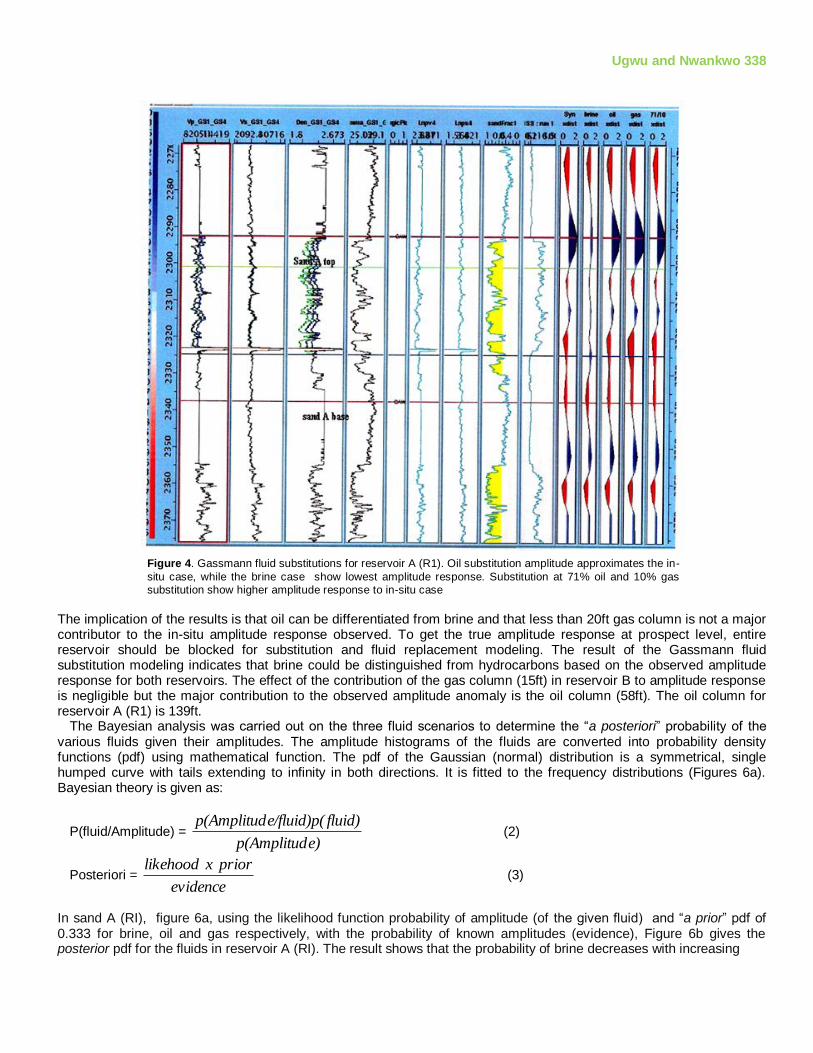
The in-situ saturation were „backed out‟ and replaced by 100% brine and then, progressively, different percentages of fluid saturations were introduced with corresponding amplitude response, for the different fluid scenarios. RESULTS AND DISCUSSION Figure 4 shows the result of fluid substitution modeling in sand A. The first synthetic is the in-situ synthetic of the reservoir containing oil and brine. 100% brine substitution shows least amplitude; at 81% oil and 19% brine substitution, the amplitude response corresponds to the in-situ scenario. However, the amplitude response increases when oil saturation is replaced with gas, and slightly increases than the in-situ case when 10% oil was replaced with gas. This result shows that the hydrocarbon could be separated from the brine, but there is slight separation between oil and gas scenarios. Non-commercial gas accumulation in this reservoir might therefore be indistinguishable from the oil scenarios on seismic. This analysis implies that the oil can be separated from the brine in terms of amplitude response at the log scale. The reservoir (sand B) contains gas, oil and brine, with the gas column less than 20ft. Figure 5a shows the substitution done on the gas zone. The in-situ synthetic has the higher response. 100% brine case shows lower amplitude response, increase in gas saturation from non-commercial saturation to commercial saturation does not lead to a corresponding increase in amplitudes; the amplitudes remain constant (from 10 to 80%), and does not approximate the in-situ case. The implication is that a gas column of 20ft will show little or no resolution on seismic and would be indistinguishable from brine accumulation. Figure 5b shows substitution carried out in the oil column. Increase in oil saturation increases the amplitude response of the synthetic. Non-commercial oil saturation (10%) has low amplitude response while commercial oil saturation (50-83%) shows a constant amplitude response. When 83% gas saturation is introduced, the amplitude increases more than that of 83% oil saturation. The result shows that in the zone of substitution, it would be difficult differentiating brine from non-commercial oil accumulation but separation is pronounced at commercial value. Like in figure 5a, none of the amplitudes approximates the in-situ case. To get the understanding of the ins-situ amplitude response and the major contributor, the entire reservoir was used as the substitution zone. Figure 5c, shows the result of this substitution. At 63% oil and 20% saturations, the amplitude response approximates that of the in-situ response, while63% gas and 20% oil saturations gives a much higher amplitude response.

Ugwu and Nwankwo 338

Figure 4. Gassmann fluid substitutions for reservoir A (R1). Oil substitution amplitude approximates the in-

situ case, while the brine case show lowest amplitude response. Substitution at 71% oil and 10% gas substitution show higher amplitude response to in-situ case

The implication of the results is that oil can be differentiated from brine and that less than 20ft gas column is not a major contributor to the in-situ amplitude response observed. To get the true amplitude response at prospect level, entire reservoir should be blocked for substitution and fluid replacement modeling. The result of the Gassmann fluid substitution modeling indicates that brine could be distinguished from hydrocarbons based on the observed amplitude response for both reservoirs. The effect of the contribution of the gas column (15ft) in reservoir B to amplitude response is negligible but the major contribution to the observed amplitude anomaly is the oil column (58ft). The oil column for reservoir A (R1) is 139ft.

The Bayesian analysis was carried out on the three fluid scenarios to determine the “a posteriori” probability of the various fluids given their amplitudes. The amplitude histograms of the fluids are converted into probability density functions (pdf) using mathematical function. The pdf of the Gaussian (normal) distribution is a symmetrical, single humped curve with tails extending to infinity in both directions. It is fitted to the frequency distributions (Figures 6a). Bayesian theory is given as:

P(fluid/Amplitude) = e)p(Amplitud

fluid)e/fluid)p(p(Amplitud (2)

Posteriori = evidence

priorxlikehood (3)

In sand A (RI), figure 6a, using the likelihood function probability of amplitude (of the given fluid) and “a prior” pdf of 0.333 for brine, oil and gas respectively, with the probability of known amplitudes (evidence), Figure 6b gives the posterior pdf for the fluids in reservoir A (RI). The result shows that the probability of brine decreases with increasing

Ugwu and Nwankwo 339

amplitudes to zero; for oil, it increases to about 70% and falls to about 20% at higher amplitudes. The gas probability increases from zero at low amplitudes

Figure 5. Gassmann fluid substitution modeling for reservoir B. 5a shows the effect of performing fluid substitution on gas column less than 20ft, no difference is observed from non commercial to commercial saturations. 5b. shows the effect of carrying out the modeling within the oil column and 5c shows the effect when the entire reservoir is modeled. In-situ amplitude response approximates 63% oil and 20% gas saturation model. Based on amplitude, brine can be separated from hydrocarbons

to about 80%. The result shows a slight chance of discriminating between the hydrocarbon types. Following the above procedures, we see from Figures 7 (c-d) that our chance of separating oil and gas is indeed small. At very high amplitudes, the probabilities that our gas and oil models are correct given their amplitudes are 0.55 and 0.45 respectively. In reservoirs, the posterior pdf for brine, oil and gas at high amplitudes are 0, <0.5 and > 0.5 respectively. AVO Classification The average rock property (Vp, Vs, ρ) values for the overlying shales, reservoir sand, gas, oil, and brine columns were obtained. Using these values and assuming an effective medium theory (Hilterman, 2001), an AVO classification was attempted for the prospect of interest (Rutherford and Williams, 1985; Castagna and Swan 1997).

Ugwu and Nwankwo 340

Figure 6 AVO modeling plots for reservoir A (RI.). (a-c) shows fluid amplitude histogram, gradient-intercept and far-near modeled plots for sand A. (d and e ) show the synthetics of 1 millisecond length for stack, intercept, gradient, offset and near and far amplitude response for the three fluid scenarios. Hydrocarbons are distinguishable from brine, but gas and oil separation is fairly difficult.

Figure 7. Bayesian probability curves for reservoirs A (R1) A (R1) and B. 7 (a and c) are

the curves for the probability of the amplitudes given the fluids, inside is the fluid

histogram used for generation of the likelihood pdf. 7 (b and d) are the posterior probability of the fluids given the amplitude. The prior probability was set at 0.333 for the three fluid scenarios

Ugwu and Nwankwo 341

Figure 8a shows an AVO plot of reflection co-efficient against angle of incidence for shale/sand A interface, and oil/brine reservoir interface. The shale/sand A (RI) shows a typical class 3-AVO effect while oil/ brine case shows a class 1-AVO effect. Figure 8b shows similar AVO plot, shale/sand B interface shows class 3-AVO effect, gas/oil and oil/brine interfaces as class 1-AVO effect. Figure 8c shows that both shale/sand A and shale/sand B are class 3-AVO case. Figure 8d is intercept gradient plot confirming that shale/reservoir A (RI) and shale/reservoir B are both class 3 AVO with negative gradient and intercept, whereas, the others (oil/brine sand A, gas/oil/brine sand B) are all Class 1-AVO with positive intercept and negative gradient. These results show that on NMO corrected CDP gathers, sand A and B would show up as class 3- AVO anomalies.

Figure 9a shows the cross plot of Lambda- rho against depth for sand A. The black ovals in the oil portion indicate shale intercalation, end member effect and hard streak. The plot reveals the hydrocarbon-water- contact (HCWC) to be gradual. The oil portion has lower incompressibility values relative to the brine portion. Figure 9b shows the cross plot of Lambda-rho against Mu-rho. As observed from Figure 9a, the oil portion cluster together with Lambda-rho values ranging from 15-25 (Gpa g/cm

3), and brine portion from 20-33 (Gpa g/cm

3). The zone of overlap shows the influence of

shale and streak. Figure 9c shows Lambda-rho against Mu-rho cross plot for the sand B. It shows the effect of end member shale (black

oval) on the thin gas cap, and further influence in the oil portion. Figure 9d shows more robustly the fluids in Lambdarho-Murho cross plot space. Gas portion has lowest incompressibility values (less than 20 Gpa g/cm

3), oil portion has fairly

high values (19-28 Gpa g/cm3), and brine portion 20-38 (Gpa g/cm

3). High λp values show the effect of end member

shale. Though the simulation showed the fluids are inseparable, the λ-μ-ρ method showed robust discrimination. The Lambdarho-dept cross plot can be effectively used to visually express the anatomy of sand A. From figure 9a

cross-plot, the qualitative behavior of the reservoir is easily noticed. The anomalous zones indicated by black ovals, corresponds to end member shale, shale intercalations and cemented sand had streak effects

Figure 8: Cross plot for AVO classification. 8 (a-c) shows the cross plot of reflection coefficient with angle of incidence for the sand reservoirs A (R1) and B. The plot reveals a class 3-AVO anomaly. 8 (d) shows the cross plot of gradient against intercept, and confirms the

characteristic AVO class of the sands, negative gradient and intercept. The fluid interface (gas/oil B, oil/brine A (R1), and oil/brine B) shows a characteristics class 1-AVO

Ugwu and Nwankwo 342

In order to explain the effectiveness of the modeled shear velocity and the measured compressional velocity within some of the reservoirs encountered, cross plot of the rock properties for Vp/Vs ratio and λρ/μρ ratio against Poisson ratio and λρ attributes respectively was set up (Figure 10). The cross plot for the two sands considered shows a more realistic Vp/Vs ratio against Poisson ratio and λp/μp ratio against λp for the oil/brine sand A(RI), than for the gas/oil/brine sand B. Relatively, the oil has low Vp/Vs and Poisson ratios, which is clearly expressed in the λρ/μρ ratio against λρ attribute space for sand A. In sand B, the gas portion tends to have higher Vp/Vs and λρ/μρratio.

Figure 9. µ-p cross plot for sands A (R1) and B 9 (a and b) shows the plots of p against depth and µp against p for reservoir A. 9 (c and d) show the same plot for sand reservoir B. Black ovals indicate the effects of end member shale, shale intercalations and hard streak. The p-depth show reveals the anatomy of the reservoir for A

Across a 3- phase fluid scenario, compressional sonic velocity drops more in the gas portion than in oil and brine, but the shear velocity does not significantly change. A reverse would have been expected in the plot of figure 10(c) and (d) for the gas/oil/brine reservoir.

Ugwu and Nwankwo 343

Figure 10. (a,b) Vp/Vs against Poisson‟s ratio cross plot and 10 (c,d) p/ µp against p cross

plot for both reservoirs. 10 b and c shows that the rock properties obtained from the well might not be correct for reservoir B, the gas sand show higher p/ µp ratio relative to that of brine which is lower. The reverse should be reasonably correct for gas sand -µ-p here proves effective in log QC

The Vp/Vs and λρ/μρ ratio clearly show this anomalous behavior. The likely effect could be attributed to the measured sonic or the modeling technique for the estimated shear sonic. The λρ/μρ ratio could therefore be effectively incorporated in the modeling to determine the fidelity of the measured and estimated well logs. AVO Modeling Gassmann fluid substitution modeling in reservoirs A and B can be discussed as follows: Reservoir RI: (i) In-situ amplitude response is much higher than brine response (ii) In-situ amplitude response is similar to 81% oil and 19% brine saturation model (iii) In-situ amplitude response is similar to 71% oil and 10% gas saturation model. (iv) In-situ amplitude response is much less than 81% gas 19% brine saturation model. Reservoirs B: (i) In-situ amplitude response is much higher than brine response (ii) In-situ amplitude response is same as 63% oil and 20% oil saturations. (iii) In-situ amplitude response is much less than 63% gas and 20% oil saturations. The results of forward modeling shows that Gassmann fluid substitution, and AVO modeling are consistent. The result suggests that hydrocarbons can be discriminated from brine, but discrimination of oil from gas is somewhat difficult. AVO analysis taking the average of Vp, Vs and density across the overlying shale and reservoir reveals that both targets of interest exhibit a Class 3-AVO anomaly.

Ugwu and Nwankwo 344

CONCLUSION

The cross plot technique proves effective in fluid discrimination within the reservoirs and can be effectively

used as a reservoir anatomy tool to check the behavior of the reservoir in the presence of fluids and artifacts. It can also be used as a quality control tool on the reliability of well log data. The Bayesian analysis shows that the posteriori probability of 50% is obtained at the overlapping zone of oil and gas in both reservoir models. At higher amplitude, the posterior probability for reservoir R1 is 0%, 15% and 85% for brine, oil and gas scenarios respectively (no gas was encountered in-situ when a residual gas saturation was modeled), and 0%, 45% and 55% respectively for reservoir B.

The result of our finding indicates that the attribute is more diagnostic of lithology, and fluid characterization for

the entire depth of inversion considered and is less affected by compaction. The implication of this modeling study is that on actual NMO corrected CDP gathers and on far seismic volumes, both should show up with increasing amplitude with offset and as bright spots. The reason why the effect of the gas column of reservoir B is quite negligible on amplitude response is that the thickness is not resolvable at seismic resolution (less than ¼ the wavelength).

ACKNOWLEDGEMENT The Authors are grateful to SPDC Port Harcourt for the provision of data used in this study, and to Mr. A.E. Gbenga for his useful contributions.

References

Aki K, Richards PG(1980). Quantitative seismology: W.H. Freeman and Co. Bachrach R, Beller M, Liu CC, Perdomo J, Shelander D, Dutta N, Benabentos M(2004). Combining rock physics analysis, full waveform prestack

inversion and high-resolution seismic interpretation to map lithology units in deep water: A Gulf of Mexico case study: The leading Edge. 4: 378-383.

Brown AR(1987). The value of seismic amplitude: The Leading Edge.10: 30 – 33. Burianyk M(2000). Amplitude-vs-offset and seismic rock property analysis: A primer: The Canadian Society of Exploration Geophysicist Recorder. 11:

1 - 14. Castagna JP, Swan HW(1997). Principle of AVO cross plotting: The Leading Edge. 4: 337-342.

Chaveste A(2003). Risk reduction in estimation of petrophysical properties from seismic data through well-log modeling, seismic modeling, and rock properties estimation: The Leading Edge. 5: 406-418.

Connoly P(1999). Elastic Impedance: The Leading Edge. 18: 438 - 452.

Dewar J(2001). Rock physics for the rest of us – An informal discussion: The Canadian Society of Exploration Geophysicist Recorder. 5: 43 – 49. Downton J, Lines L(2001). AVO feasibility and reliability analysis in the presence of random noise: The Recorder. 66: 66-73. Ekweozor M, Daukoru EM(1994). Northern delta depobelt portion of the Akata-Agbada(!) petroleum system, Niger Delta, Nigeria, in, Magoon, L.B.,

and Dow, W.G., eds., The petroleum system- From Source to Trap, AAPG Memoir 60: Tulsa, American Association of Petroleum Geologists. Pp. 599-614.

Fatti JL, Smith GC, Vail PL, Strauss PJ, Levitt PR(1994). Detection of gas in sandstone reservoirs using AVO analysis: A 3-D seismic case history

using the Geostack technique: Geophysics. 59: 1352 – 1376. Goodway B (2001). AVO and Lame constants for rock parameterization and fluid detection: The Canadian Society of Exploration Geophysicist

Recorder. 6: 39 – 60.

Goodway B, Chen T, Downton J(1997). Improved AVO fluid detection and lithology discrimination using Lame petrophysical parame ters: λρ, μρ and λ/μ fluid stack, from P, and S, inversions: presented at the 6

th Ann. Interna, Mtg., SEG, Expanded Abstracts. 183 – 186.

Henry S(2006). Undestanding seismic amplitudes: www.searchanddiscovery.net

Hilterman FJ (1990). Is AVO the seismic signature of lithology? A case study of ship shoal – South Addition: The Leading Edge. 6: 15 – 22. Hilterman FJ(2001). Seismic Amplitude Interpretation, 2001, Distinguished instructor short course, Distinguish instructor series, No, 4, Soc., Expl.

Geophys.

Mallick S, Lauve J, Ahmed R(2000). Hybrid seismic inversion: A Reconnaissance tool for deep – water exploration: Western Geophysical, Houston. 36 – 43.

Orife JM, Avbovbo AA(1982). Stratigraphic and unconformity traps in the Niger Delta: AAPG Bulletine. 66(2): 251-262.

Ostrander WJ(1984). Plane – wave reflection coefficients for gas sands at non-normal angles of incidence: Geophysics. 49: 1637 – 1648. Quakenbush M, Shang B, Tutle C(2006). Poisson impedance: The Leading Edge. 25: 128 – 139. Reijers TJA, Peter SW, Nwajide CS(1996). The Niger Delta basin: In Reijers, T.J.A., ed., : Selected Chapter on Geology: SPDC Warri. Pp. 103-118.

Ross CP(2000). Effective AVO crossplot modeling: A tutorial: Geophysics. 65: 700 – 711. Russell BH, Hedlin K, Hilterman FJ, Lines LR(2003). Fluid property discrimination with AVO: A Biot-Gassmann perspective: Geophysics. 68: 29-39. Rutherford SR, Williams RH(1985). Amplitude – versus – offset variations in gas sands: Geophysics. 54: 680 – 688.

Shuey RT(1985). A simplification of the Zoeppritz equations: Geophysics. 50: 609 – 614. Smith GC, Gildow PM(1987). Weighted stacking for rock property estimation and detection of gas: Geophysical prospecting. 35: 993 – 1014. Smith MT, Sondergeld HC, Rai SC(2003). Gassmann fluid substitutions: A tutorial: Geophysics. 68: 430-440.

Tuttle MLW, Charpentier RR, Brownfield ME(1999). The Niger Delta petroleum system: Niger Delta province, Cameroon, and Equatorial Guinea, Africa:http://greenwood.cr.usgs.gov/energy/WorldEnergy/OF99-50H/ChapterA.htm#TOP

Veeken PCH, Rauch M(2006). AVO attribute analysis and seismic reservoir characterization. First break. 24: 41-52.

Walls J, Dvorkin J, Carr M(2005). Well logs and rock physics in seismic reservoir characterization: www.rocksolidimages.com. Yang GYC, Stewart RR(1997). Linking petrophysical parameters with seismic parameters: Consortium for Research in Elastic Wave Exploration

Seismology Report. 9(7): 1-9.

Ziolkowshi A, Underhill RJ, Johnston GKR(1998). Wavelets, Well ties and the search for subtle stratigraphic traps: Geophysics. 63: 297-313.