fluid-structure interaction problems in hemodynamics: parallel
TRANSCRIPT
POUR L'OBTENTION DU GRADE DE DOCTEUR ÈS SCIENCES
acceptée sur proposition du jury:
Prof. K. Hess Bellwald, présidente du juryProf. A. Quarteroni, Dr S. Deparis, directeurs de thèse
Dr M. Picasso, rapporteur Dr C. Vergara, rapporteur
Fluid-Structure Interaction Problems in Hemodynamics: Parallel Solvers, Preconditioners, and Applications
THÈSE NO 5109 (2011)
ÉCOLE POLYTECHNIQUE FÉDÉRALE DE LAUSANNE
PRÉSENTÉE LE 25 JUILLET 2011
À LA FACULTÉ SCIENCES DE BASECHAIRE DE MODÉLISATION ET CALCUL SCIENTIFIQUE
PROGRAMME DOCTORAL EN MATHÉMATIQUES
Suisse2011
PAR
Paolo CROSETTO

ii

Riassunto
I principali obiettivi di questo lavoro sono la descrizione, lo studio e la simulazione numericadel problema di interazione fluido–struttura (FSI) applicato all’emodinamica (dinamica delsangue) nelle arterie. Lo studio numerico dell’emodinamica nel sistema cardiovascolare e unsoggetto di ricerca molto attivo, in quanto permetterebbe, una volta validato, di predire l’in-sorgere di patologie, di scegliere la terapia piu’ opportuna o di comprendere meglio l’influenzadi fattori (come lo sforzo di taglio a parete o wall shear stress, WSS) notoriamente legati allanascita di disturbi (come l’ateroscerosi).
Questo lavoro e suddiviso in tre parti, formate da due capitoli ciascuna. Nella primaparte vengono ricavate le equazioni differenziali che costituiscono il problema accoppiato: leequazioni di Navier–Stokes in un dominio mobile per il fluido (sangue), viscoso e incom-primibile, l’equazione dell’elasticita per la struttura (parete arteriosa). In particolare vienedescritta in dettaglio la rappresentazione delle equazioni del fluido in un sistema di riferi-mento Lagrangiano–Euleriano arbitrario (ALE), una scelta frequente in ambito FSI che verraadottata nei capitoli successivi. In seguito vengono introdotte le condizioni di accoppiamen-to, ovvero le continuita della velocita e degli sforzi all’interfaccia tra fluido e struttura (lasuperficie endoteliale della parete arteriosa). Nella prima parte vengono discusse anche ladiscretizzazione spaziale in elementi finiti (FE) e temporale del sistema FSI. Questa discretiz-zazione permette di rappresentare il sistema di equazioni in uno spazio di dimensione finita,dando luogo ad un sistema discreto la cui soluzione e unica. La scelta della discretizzazionetemporale coinvolge due aspetti: la discretizzazione in tempo dei due problemi (fluido e strut-tura) e quella delle condizioni di accoppiamento (continuita delle velocita e degli sforzi). Perentrambi gli aspetti la scelta puo influire sulla stabilita del sistema discreto. Alla fine dellaprima parte di questa tesi viene riportata una descrizione dello stato dell’arte, focalizzatasuilla stabilita del sistema.
Il sistema di equazioni discretizzato e nonlineare. In particolare la dipendenza del domimiofluido dallo spostamento della struttura e la formulazione ALE scelta per il fluido introduconouna forte nonlinearita, il cui trattamento costituisce uno dei due principali argomenti dellaseconda parte della tesi. In letteratura la nonlinearita del sistema FSI viene frequentementerisolta per mezzo del metodo di punto fisso, che ha come vantaggi robustezza ed implementa-zione relativamente immediata, ma anche, nella sua implementazione classica, lo svantaggio diessere inefficiente in alcune circostanze (tipicamente per esempio nel caso dell’emodinamica).Un algoritmo piu efficace, che viene utilizzato in questo lavoro, e quello di Newton. La mag-giore difficolta di questo approccio consiste nel calcolo della matrice Jacobiana, che richiedela valutazione delle derivate dei termini nonlineari. In particolare la nonlinearita dovuta alladipendenza del dominio fluido dallo spostamento della struttura fa intervenire delle derivatedi forma nello Jacobiano del sistema. Il calcolo analitico e l’assemblaggio di queste derivatenella matrice Jacobiana non sono banali (questi termini sono spesso trascurati o approssimati
numericamente in letteratura), e vengono descritti nel terzo capitolo. Considerazioni orienta-te all’implementazione di questa parte in un codice ad elementi finiti sono riportate alla finedel capitolo e costituiscono un contributo originale di questo lavoro.
La seconda parte prosegue, nel quarto capitolo, con lo studio dei metodi di risoluzionedel sistema lineare (Jacobiano). Un metodo efficace solitamente adottato per questo tipodi sistemi (grandi, sparsi e non simmetrici) e GMRES, un metodo di Krylov matrix–free,che richiede soltanto delle moltiplicazioni matrice–vettore per la soluzione del sistema. So-litamente questo metodo e utilizzabile in applicazioni pratiche soltanto se precondizionato.Dopo una rassegna sui metodi comunemente usati in FSI per risolvere il sistema linearizzatoviene proposto un nuovo tipo di precondizionatori, che permette di trattare separatamentei blocchi corrispondenti ai diversi problemi (fluido e struttura). Un’analisi di questo tipodi precondizionatori, proposta alla fine della seconda parte, mostra che il condizionamentodel sistema globale precondizionato dipende in gran parte dal condizionamento dei singoliproblemi disaccoppiati.
Nella terza parte i metodi descritti nei capitoli precedenti vengono applicati a dei casiclinici. Sono simulati diversi battiti cardiaci in un arco aortico ed in un bypass femorale.Viene calcolato il WSS, vengono messi a confronto diversi metodi (modelli 1D, con pareterigida ed FSI) e diverse discretizzazioni spaziali e temporali. Infine, nell’ultimo capitolo,sono presentati risultati di scalabilita forte e debole su diverse griglie, utilizzando diversediscretizzazioni temporali. Le simulazioni di questo capitolo sono state lanciate su piattaformeparallele ad alta performance (Cray XT5, Cray XT6, Blue Gene/P).
ii

Resume
Les objectifs de ce travail sont la description, l’etude et la simulation numerique duprobleme d’interaction fluide–structure (FSI) applique a la dynamique du sang (hemodynamique)dans les arteres. L’etude numerique du systeme cardiovasculaire d’un point de vue hemodynamiqueest un sujet de recherche tres actif, permettant, une fois valide, de predire le developpementde pathologies (par example l’atherosclerose), de mieux comprendre l’influence de facteurs(comme le wall shear stress, WSS) qu’y sont associes et de l’appliquer a la pratique clinique.
Ce travail est divise en trois parties, chacune formee de deux chapitres. Dans la premierepartie les equations differentielles qui constituent le probleme couple sont introduites : lesequations de Navier–Stokes dans un domaine deformable pour le fluide (sang), visqueuxet incompressible, l’equation de l’elasticite pour la structure (paroi arterielle). En particu-lier on decrit en detail la representation des equations du fluide dans un repere arbitraireLagrangien-Eulerien (ALE), un choix frequent en FSI qui sera adopte durant cette these. En-suite on decrit les conditions de couplage : continuite des vitesses et des contraintes a l’interfacefluide–structure. On introduit egalement dans la premiere partie les discretisations spatiale,en elements finis, et temporelle du systeme FSI. Ces discretisations permettent de representerle systeme d’equations dans un espace de dimension finie, ce qui mene a un probleme discretdont la solution est unique. Le choix de la discretisation temporelle influence deux aspects :la discretisation en temps des deux problemes (fluide et structure) et celle des conditionsde couplage (continuite des vitesses et des contraintes). Pour les deux aspects le choix peutaffecter la stabilite du systeme discret. Une description concernant en particulier la stabilitedu systeme se trouve a la fin de la premiere partie de ce travail.
Le systeme d’equations discretise n’est pas lineaire, le fait que le domaine du fluide dependedu deplacement de la structure, ainsi que la formulation ALE pour le fluide, introduisent uneforte nonlinearite dont le traitement est un des deux arguments principaux de la deuxiemepartie de cette these. Il est souvent propose dans la litterature de resoudre la nonlinearite dusysteme FSI en appliquant la methode du point fixe. Elle a pour avantages d’etre robuste etd’avoir une implementation assez simple. Par contre, dans sa forme classique, cette methodepresente le desavantage de ne pas etre efficace dans tous les cas, notamment l’hemodynamique.Un algorithme plus performant, qui est utilise dans ce cas, est celui de Newton. La difficulteprincipale de cette methode vient du calcul de la matrice Jacobienne, qui requiert l’evaluationdes derivees des termes nonlineaires. En particulier, la nonlinearite due a la dependance dudomaine fluide du deplacement de la la structure fait intervenir des derivees de forme dans leJacobien du systeme. Le calcul analytique et l’assemblage de ces derivees ne sont pas triviaux(ces termes sont souvent negliges ou approximes dans la litterature), et sont decrits dans letroisieme chapitre. A la fin de ce chapitre on decrit l’implementation de cette partie dans uncode aux elements finis, ce qui constitue une contribution originale de ce travail.
Dans le quatrieme chapitre on etudie des methodes de resolution du systeme lineaire (Ja-

cobien). Une methode efficace normalement utilisee pour ce type de systemes (grands, creuxet nonlineaires) est GMRES. Cette methode est utilisee normalement dans les cas pratiquesavec un preconditionneur. Apres avoir resume des methodes utilisees en FSI pour resoudrele systeme lineairise, un nouveau type de preconditionneurs est propose. Ces precondition-nerus permettent de traiter separement les blocs qui correspondent aux problemes differents(comme fluide et structure). Une analyse proposee pour ce type de preconditionneurs montreque le conditionnement du systeme global preconditionne ne depend que du conditionnementdes problemes decouples.
Dans la troisieme partie, les methodes decrites dans les chapitres precedents sont ap-pliquees a des cas cliniques. Plusieurs battements cardiaques consecutifs sont simule dans lecas de l’aorte thoracique d’un sujet sain, ainsi que dans le cas d’un pontage femoro–poplite.Le WSS est calcule et differentes methodes sont comparees (modele 1D, paroi rigide, FSI),ainsi que differentes discretisations spatiales et temporelles. Enfin dans le dernier chapitre, lesresultats de scalabilite forte et faible sont montres, sur des maillages differents, avec differentesmethodes. Les simulations de ce chapitre ont ete realisees sur des clusters a haute performance(Cray XT5, Cray XT6, Blue Gene/P).
Mots cle : Interaction fluide-structure, preconditionneurs paralleles, hemodynamique,elements finis
iv

Abstract
In this work we aim at the description, study and numerical investigation of the fluid–structureinteraction (FSI) problem applied to hemodynamics. The FSI model considered consists ofthe Navier–Stokes equations on moving domains modeling blood as a viscous incompressiblefluid and the elasticity equation modeling the arterial wall. The fluid equations are derivedin an arbitrary Lagrangian–Eulerian (ALE) frame of reference. Several existing formulationsand discretizations are discussed, providing a state of the art on the subject. The main newcontributions and advancements consist of:
• A description of the Newton method for FSI–ALE, with details on the implementationof the shape derivatives block assembling, considerations about parallel performance,the analytic derivation of the derivative terms for different formulations (conservativeor not) and for different types of boundary conditions.
• The implementation and analysis of a new category of preconditioners for FSI (appli-cable also to more general coupled problems). The framework set up is general andextensible. The proposed preconditioners allow, in particular, a separate treatment ofeach field, using a different preconditioning strategy in each case. An estimate for thecondition number of the preconditioned system is proposed, showing how precondition-ers of this type depend on the coupling, and explaining the good performance theyexhibit when increasing the number of processors.
• The improvement of the free (distributed under LGPL licence) parallel finite elementslibrary LifeV. Most of the methods described have been implemented within this libraryduring the period of this PhD and all the numerical tests reported were run using thisframework.
• The simulation of clinical cases with patient–specific data and geometry, the compari-son on simulations of physiological interest between different models (rigid, FSI, 1D),discretizations and methods to solve the nonlinear system.
A methodology to obtain patient–specific FSI simulations starting from the raw medicaldata and using a set of free software tools is described. This pipeline from imaging to simu-lation can help medical doctors in diagnosis and decision making, and in understanding theimplication of indicators such as the wall shear stress in the pathogenesis.
Keywords: Fluid-structure interaction, parallel preconditioners, hemodynamic, finiteelements

vi

A nonna Rita


Acknowledgments
During my PhD I was fascinated by the new parallel architectures which keep improving interms of speed, size and energy consumption. My conclusion, at the end of three years (≈)is that the most performant parallel machine is here at the EPFL. It’s my supervisor Prof.Alfio Quarteroni: no matter how much the workload increases, he manages to be up to datewith everybody’s work, to send suggestions, corrections, so I guess he meets the definition ofweak scalability. I would like to thank him also for his capability of understanding how todeal with each one of his students, in order to get the best possible outcome.
Secondly, I want to thank my other supervisor, Dr. Simone Deparis, who looked after mefor all this period, forgiving me all my forgetfulness. Besides the outstanding professionalskills, he is a person with a deep humanity and a magic capability of “breaking the ice” witha laugh and taking it easy.
A huge thanks goes to my family: my mother Irene, father Alberto, sister Elena and mygrandma Margherita for the provisions of good food, wine, clothes, and for being availablefor any problem and supportive in any circumstances.
I want to thank the CMCS crew, I am sure that I could find plenty of qualities for allof them, from both the professional and human points of view. I just acknowledge explicitlyJean for correcting all the accents in the resume, Claudia, who had the “luck” of reading thefirst part of this thesis at an early stage (and gave me several corrections), and Radu, whois already a celebrity in Moretta, for a list of moments ranging from Sat’s Karmeliet to thehistorical B-fest. I did not forget the people who left the crew, in particular Annalisa, withher smiles and complaints, Lausanne is less colorful ever since she went to Texas.
Among the the “swiss” people I want to thank Elena, Ale and Ojas, historical friends, itseems to me that I known them since forever. Among the “italians” I’d like to thank Davideand Alexandra for having left for me a spot on their couch in Torino, every Friday when Iwas back from Lausanne, Andrea (prugna), probably the most honest person on the face ofearth, and the B-team. Thanks also to Chiara and Cristina, that I just crossed during thisperiod, but I have wonderful souvenirs of them.
Thanks to the owners of the arteries simulated during this thesis: Dr. Philippe Rey-mond, whose passion for research always motivates me, and who contributed to many resultscontained in the simulations section, and Monsieur Martin. Thanks also to Gilles, who wasgenerous of precious contributions and suggestions. I acknowledge the Swiss National ScienceFoundation grant 200020-117587 for the support, CSCS, HECToR, CADMOS and DIT forthe availability of the supercomputers, the European grant Mathcard, the Swiss Platform forHigh-Performance and High-Productivity Computing (HP2C).
Eventually I would like to thank my coffee machine Alicia, and the “head scratcher” (thosewho spent some time in my office know how much support they gave me).


Contents
I Physics of the Problem 7
Derivation of the Equations for Fluid and Structure 91.1 The Kinematics of Continuous Media . . . . . . . . . . . . . . . . . . . . . . . 91.2 Lagrangian, Eulerian and ALE Formulations . . . . . . . . . . . . . . . . . . 131.3 The Equations of Continuum Mechanics . . . . . . . . . . . . . . . . . . . . . 161.4 The Equations for a Fluid . . . . . . . . . . . . . . . . . . . . . . . . . . . . . 191.5 The Equations for a Solid . . . . . . . . . . . . . . . . . . . . . . . . . . . . . 21
Modeling Fluid–Structure Interaction Problems 252.1 Coupling Conditions . . . . . . . . . . . . . . . . . . . . . . . . . . . . . . . . 252.2 Three Fields Formulation . . . . . . . . . . . . . . . . . . . . . . . . . . . . . 262.3 Time Discretization for the Structure Problem . . . . . . . . . . . . . . . . . 282.4 Time Discretization for the Fluid–Geometry Problem . . . . . . . . . . . . . . 292.5 Fully Implicit and Convective Explicit Schemes . . . . . . . . . . . . . . . . . 322.6 Geometry–Convective Explicit Scheme . . . . . . . . . . . . . . . . . . . . . . 322.7 Space Discretization . . . . . . . . . . . . . . . . . . . . . . . . . . . . . . . . 33
2.7.1 Interior Penalty Stabilization . . . . . . . . . . . . . . . . . . . . . . . 382.8 Analysis of the Coupled Problem . . . . . . . . . . . . . . . . . . . . . . . . . 38
2.8.1 Analysis of Simplified Coupled Models . . . . . . . . . . . . . . . . . . 382.8.2 Stability and Geometric Conservation Law . . . . . . . . . . . . . . . 402.8.3 Strong versus Weak Coupling . . . . . . . . . . . . . . . . . . . . . . . 42
Added Mass Effect . . . . . . . . . . . . . . . . . . . . . . . . . . . . . 42Fractional–Step and Explicit Couplings . . . . . . . . . . . . . . . . . 45
2.9 Geometrical Multiscale . . . . . . . . . . . . . . . . . . . . . . . . . . . . . . . 46
II Solution Strategies for the FSI problem 49
Nonlinearities and Newton Method 513.1 Newton Method . . . . . . . . . . . . . . . . . . . . . . . . . . . . . . . . . . . 513.2 Fixed Point Formulations . . . . . . . . . . . . . . . . . . . . . . . . . . . . . 52
3.2.1 Dirichlet–Neumann Formulation . . . . . . . . . . . . . . . . . . . . . 543.2.2 Steklov–Poincare Formulation . . . . . . . . . . . . . . . . . . . . . . . 56
3.3 Newton Method for Geometrical Multiscale . . . . . . . . . . . . . . . . . . . 603.4 Computing the Exact Jacobian Matrix . . . . . . . . . . . . . . . . . . . . . . 61
3.4.1 Shape Derivatives of Domain Functionals . . . . . . . . . . . . . . . . 62

CONTENTS
3.4.2 Shape derivatives in FSI-ALE . . . . . . . . . . . . . . . . . . . . . . . 653.4.3 Implementation . . . . . . . . . . . . . . . . . . . . . . . . . . . . . . . 69
Solution of the Algebraic Linear System 714.1 Block Triangular Preconditioners . . . . . . . . . . . . . . . . . . . . . . . . . 71
4.1.1 Schur Complement Preconditioners . . . . . . . . . . . . . . . . . . . . 724.1.2 Block Gauss–Seidel Preconditioners . . . . . . . . . . . . . . . . . . . 74
4.2 Applications to the FSI system . . . . . . . . . . . . . . . . . . . . . . . . . . 744.2.1 Robin–Robin Preconditioners . . . . . . . . . . . . . . . . . . . . . . . 774.2.2 Dirichlet–Dirichlet Preconditioners . . . . . . . . . . . . . . . . . . . . 794.2.3 Other Additive Preconditioners . . . . . . . . . . . . . . . . . . . . . . 814.2.4 Extension to Other Time Discretizations . . . . . . . . . . . . . . . . . 82
4.3 Parallel Preconditioners for FSI . . . . . . . . . . . . . . . . . . . . . . . . . . 844.3.1 State of the Art . . . . . . . . . . . . . . . . . . . . . . . . . . . . . . 854.3.2 Composed Preconditioners for Geometry–Convective Explicit FSI . . . 874.3.3 Composed Preconditioners for Geometry Implicit FSI . . . . . . . . . 884.3.4 Spectral Analysis . . . . . . . . . . . . . . . . . . . . . . . . . . . . . . 89
III Applications and Simulations 95
Applications to Hemodynamics 975.1 Applications and Motivation . . . . . . . . . . . . . . . . . . . . . . . . . . . 97
5.1.1 Circulation . . . . . . . . . . . . . . . . . . . . . . . . . . . . . . . . . 975.1.2 Cardiovascular Diseases . . . . . . . . . . . . . . . . . . . . . . . . . . 99
5.2 Problem Description . . . . . . . . . . . . . . . . . . . . . . . . . . . . . . . . 1015.2.1 From DICOM Images to Numerical Simulations . . . . . . . . . . . . 1025.2.2 Unsteady Blood Flow in a Compliant Iliac Artery . . . . . . . . . . . 104
5.3 Quality Mesh Generation for Cardiovascular Flow Simulations . . . . . . . . . 1055.3.1 Surface Remeshing Techniques . . . . . . . . . . . . . . . . . . . . . . 106
Harmonic Mapping . . . . . . . . . . . . . . . . . . . . . . . . . . . . . 107Conformal Mapping . . . . . . . . . . . . . . . . . . . . . . . . . . . . 107
5.3.2 High Quality Meshes . . . . . . . . . . . . . . . . . . . . . . . . . . . . 1075.3.3 Unsteady Blood Flow in a Compliant Femoropopliteal Bypass . . . . . 110
5.4 Blood Flow in the Aorta . . . . . . . . . . . . . . . . . . . . . . . . . . . . . . 1125.4.1 Boundary Conditions . . . . . . . . . . . . . . . . . . . . . . . . . . . 1145.4.2 Geometrical Model . . . . . . . . . . . . . . . . . . . . . . . . . . . . . 1175.4.3 Timings and Validation for FSI (GCE) . . . . . . . . . . . . . . . . . . 1185.4.4 Numerical Assessment . . . . . . . . . . . . . . . . . . . . . . . . . . . 1255.4.5 Wall Shear Stress . . . . . . . . . . . . . . . . . . . . . . . . . . . . . . 125
5.5 Comparisons . . . . . . . . . . . . . . . . . . . . . . . . . . . . . . . . . . . . 1295.5.1 GCE versus FI . . . . . . . . . . . . . . . . . . . . . . . . . . . . . . . 1295.5.2 Exact versus Inexact Newton Method . . . . . . . . . . . . . . . . . . 1475.5.3 FSI (GCE) versus Rigid Walls and 1D . . . . . . . . . . . . . . . . . . 149
xii

CONTENTS
Scalability and Parallel Performances 1516.1 Introduction . . . . . . . . . . . . . . . . . . . . . . . . . . . . . . . . . . . . . 1516.2 Scalability and Results . . . . . . . . . . . . . . . . . . . . . . . . . . . . . . . 151
6.2.1 Strong Scalability Tests . . . . . . . . . . . . . . . . . . . . . . . . . . 152Strong Scalability for GCE . . . . . . . . . . . . . . . . . . . . . . . . 153Strong Scalability for CE . . . . . . . . . . . . . . . . . . . . . . . . . 154Physiological geometries . . . . . . . . . . . . . . . . . . . . . . . . . . 157
6.2.2 Weak Scalability Test . . . . . . . . . . . . . . . . . . . . . . . . . . . 158Weak Scalability for GCE . . . . . . . . . . . . . . . . . . . . . . . . . 159Weak scalability for CE . . . . . . . . . . . . . . . . . . . . . . . . . . 162Conclusion . . . . . . . . . . . . . . . . . . . . . . . . . . . . . . . . . 162
xiii

Introduction
The modeling of the cardiovascular system is receiving increasing attention from both themedical and mathematical environments because of, from the one hand, the great influence ofhemodynamics on cardiovascular diseases and, from the other hand, its challenging complexitythat keeps open the debate about the setting up of appropriate models and algorithms. Awide variety of approaches can be found in literature, dealing with different formulations ofthe problem and solution strategies.
Below we give an overview of some of the most popular methodologies to solve numericallythe system of equations arising from the hemodynamic model. We briefly introduce thecoupled Fluid–Structure Interaction (FSI) problem, listing many of the different approachescommonly adopted to tackle it. We also report an outline of the thesis, which is concernedwith the development of algorithms for the solution of the FSI problem and their applicationto blood flow in situations of clinical relevance.
The equations considered in the present work consist of those describing the flow fieldvariables (blood velocity and pressure) and those that govern the mechanical deformation ofthe “structure” (the vessel walls). The first distinction between the different methodologiescomes from the formulation of the problem.
A common choice in the FSI context is to describe the fluid equations using an ArbitraryLagrangian-Eulerian (ALE) frame of reference (see e.g. [Nob01, SH07], cf. Chapter 1). Theadvantage with respect to an Eulerian description is that the coupling can be satisfied exactlyon the fluid-structure interface. However the introduction of a new equation for the fluiddomain motion is required, and its dependence on the solution of the FSI problem introducesa further nonlinearity.
A different approach consists of using a space-time formulation within an Eulerian frame-work. Usually, the latter involves a discretization of the computational domain in time slabs,and each solution in a time slab is computed sequentially (see [TSS06, HWD04], or [BCHZ08]for a description of this formulation).
Other approaches are based on a standard Eulerian formulation [CMM08, WCLB08,MPGW10]. With the latter approach the computation of the fluid domain displacementis avoided, however a method to keep track of the fluid-structure interface must be employed.
Also the Lagrangian meshless finite elements methods [IOP03, OnO11] have been coupledwith structure equations in order to model FSI problems. The dynamic of the fluid is mod-eled in a Lagrangian frame of reference, which has the advantage that the convective termdisappears and the disadvantage that at each time step the domain discretization needs to berecomputed.
The lattice Boltzmann method, quite popular in computational fluid dynamics, has re-cently been used also for FSI. The coupling with a finite elements method for the struc-
CONTENTS
ture mechanics is investigated e.g. in [Kwo08], while the immersed boundary method is usedin [CZ10] to identify the fluid-structure interface.
Once the system of equations describing the physical problem is set up, a further optionalstep consists of splitting the global system into subdomain problems, one domain being thatof the fluid, the other that of the solid, within standard domain decomposition (DD) ap-proaches. In this context, Dirichlet–Neumann schemes are the most popular ones adoptedin FSI (see e.g. [BQQ08a, KW08b, DDFQ07, MNS06, FM05]). Robin-Neumann and Robin-Robin schemes are applied in [BNV08, GGNV10] to the FSI context, while other standarddomain decomposition strategies (e.g. Neumann-Neumann, FETI) are described for a generalproblem e.g. in [TW05]. Another similar option consists of reformulating the problem on thefluid-structure interface through the Steklov–Poincare operators, see e.g. [DDQ06, DDFQ06].
All these strategies correspond to a particular choice of the subdomains and of the interfaceconditions assigned in the course of the subdomain iterations. Following the definitions givenin [CK02] all these formulations of the problem can be qualified as nonlinear preconditioners(see Section §3.2). These domain decomposition schemes are particularly suited to the casewhen separate (and independent) solvers for the subdomain problems are available, becausethe solution of the global system can be obtained through repeated solutions of the subdomainproblems (this property is often referred to as modularity).
The choice of the time discretization introduces further distinctions among the meth-ods. The fully coupled nonlinear problem can be discretized in time by considering all theterms in the equations implicitly, which leads to a Fully Implicit (FI) method [BCHZ08,TSS06, HHB08, KGF+09, BC10a, DP07]. This is the most stable but also most expensivechoice. A large variety of alternative time discretizations can be devised. For instance aGeometry-Convective Explicit (GCE) discretization is proposed in [BQQ08a], where the mov-ing geometry is taken at the previous time step and the convective term is treated partlyexplicitly (see Section §2.7 for details). Even in the space-time framework the fluid domainin a time slab can be extrapolated using the informations relative to previous time slabs,e.g. [TSS06, HWD04]. In this thesis (cf. Chapter 5) we compare the FI and GCE methods,together with two other intermediate options, obtained by varying the time discretization ofthe convective term.
A natural way to handle the nonlinearity is based on the use of the Aitken acceleratedfixed point algorithm in all its variants, see e.g. [KW08b, BQQ08a, DDFQ06]. In this wayeach fixed point iteration requires one residual evaluation.
Otherwise the time discretized problem can be linearized via the Newton method, eitherconsidering the full Jacobian matrix, as in [BCHZ08, HHB08, FM05, TSS06, GKW10], orneglecting some of its contributions, as in [BC10a, GV03, DBV09, Hei04, Dep04]. In theNewton method the full Jacobian matrix is often available only as matrix-vector multiplication(this is the case in [FM05] and in [GKW10]). In these cases a matrix–free method must beemployed to solve exactly the Jacobian system. Each iteration of this method requires asolve of the linearized subproblems. Thus the cost of each nonlinear iteration correspondsto the cost of one residual evaluation plus a variable number of solutions of the linearizedsubproblems. A detailed explanation of this kind of algorithms is provided in Chapter 3.
A further distinction between the different methods comes from the way the couplingconditions are advanced in time. We can devise three main different coupling strategies:strong coupling, weak coupling, fractional step schemes, see Section §2.8.3. This choice hasan impact on both the stability and the order of accuracy of the overall scheme.
For what concerns the fully coupled discretized equations where no domain decomposi-
2
CONTENTS
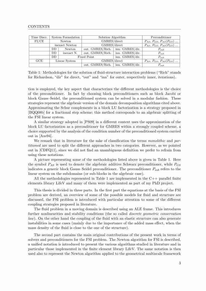
Time Discr. System Formulation Solution Algorithm Preconditioner
FI/CE Newton GMRES/direct PAS , PGS , PAS(PGS) ...
inexact Newton GMRES/direct PAS , PGS , PAS(PGS) ...
DD Newton out. GMRES/Rich. inn. GMRES/dir. PsubDD inexact N. out. GMRES/Rich. inn. GMRES/dir. PsubDD Fixed Point inn. GMRES/dir. Psub
GCE Linear System GMRES/direct PAS , PGS , PAS(PGS) ...
out. GMRES/Rich. inn. GMRES/dir. Psub
Table 1: Methodologies for the solution of fluid-structure interaction problems (“Rich” standsfor Richardson, “dir” for direct, “out” and “inn” for outer, respectively inner, iterations).
tion is employed, the key aspect that characterizes the different methodologies is the choiceof the preconditioner. In fact by choosing block preconditioners such as block Jacobi orblock Gauss–Seidel, the preconditioned system can be solved in a modular fashion. Thesestrategies represent the algebraic version of the domain decomposition algorithms cited above.Approximating the Schur complements in a block LU factorization is a strategy proposed in[BQQ08b] for a fractional step scheme; this method corresponds to an algebraic splitting ofthe FSI linear system.
A similar strategy adopted in [PS09] in a different context uses the approximation of theblock LU factorization as a preconditioner for GMRES within a strongly coupled scheme, achoice supported by the analysis of the condition number of the preconditioned system carriedout in [Axe94].
We remark that in literature for the sake of classification the terms monolithic and par-titioned are used to split the different approaches in two categories. However, as we pointedout in [CDFQ11], since we did not find an unambiguous definition we prefer to refrain fromusing these notations.
A picture representing some of the methodologies listed above is given in Table 1. Herethe symbol PAS is used to denote the algebraic additive Schwarz preconditioner, while PGSindicates a generic block Gauss–Seidel preconditioner. The preconditioner Psub refers to thelinear system on the subdomains (or sub-blocks in the algebraic case).
All the methodologies represented in Table 1 are implemented in the C++ parallel finiteelements library LifeV and many of them were implemented as part of my PhD project.
This thesis is divided in three parts. In the first part the equations at the basis of the FSIproblem are derived, an overview of some of the possible models for fluid and structure arediscussed, the FSI problem is introduced with particular attention to some of the differentcoupling strategies proposed in literature.
The fluid problem in a moving domain is described using an ALE frame. This introducesfurther nonlinearities and stability conditions (the so called discrete geometric conservationlaw). On the other hand the coupling of the fluid with an elastic structure can also generateinstabilities in some cases (mainly due to the importance of the added mass effect, when themass density of the fluid is close to the one of the structure).
The second part contains the main original contributions of the present work in terms ofsolvers and preconditioners for the FSI problem. The Newton algorithm for FSI is described,a unified notation is introduced to present the various algorithms studied in literature and inparticular those implemented in the finite element library LifeV. The same notation is thenused also to represent the Newton algorithm applied to the geometrical multiscale framework
3
CONTENTS
(i.e., the coupling of 3D FSI models with 1D models for arteries). Special attention is devotedto the derivation of the full Jacobian matrix of the whole FSI problem. This Jacobian includesa block containing cross derivatives of the fluid equations with respect to the domain motion.These (shape) derivatives have a non-trivial expression whose derivation is usually omittedfor the sake of simplicity. We report here in Section §3.4 all the calculations leading to theexpression of these derivatives together with implementation-oriented observations, whichenhance the scalability and efficiency of the current approach.
The preconditioning techniques for FSI are discussed and an overview of the classical pre-conditioning strategies used in this field is provided. A preconditioning strategy is introducedwhich consists in a combination of block Gauss–Seidel and domain decomposition precondi-tioners. This technique allows to split the preconditioner in as many factors as the numberof sub problems considered and for this reason it is well suited for multiphysics problems.The preconditioner is obtained as the product of the preconditioners built for each factor.Each one of these factors may then, in their turn, exploit a preconditioning strategy tunedfor the specific problem, and if a factor does not change during the whole simulation thecorresponding preconditioner can be reused, saving computational time. An estimate for thecondition number of the preconditioned system is derived, showing that it depends on thequality of the preconditioners for each single factor in the aforementioned factorization andon the maximum singular value of a specific matrix, whose form depends on one of the cou-pling blocks (cf. Section §4.3.4). We remark that this maximum singular value plays a rolesimilar to the CBS constant (see [KM09, AK10, Axe94], cf. Chapter 4), but it is not tied tosymmetric positive definite matrices.
The third part of this thesis contains the numerical simulations as well as a comparisonin terms of computational efficiency and accuracy of the results obtained using differentsolvers and preconditioners here proposed. The application domain is the hemodynamicin large arteries. Our simulations concern the blood dynamics in a compliant aortic archunder physiological conditions and in a femoropopliteal bypass, equipped with boundaryconditions taken from clinical measurements. The results show that the values of relevanthemodynamic factors such as the wall shear stress (WSS), an important indicator for severaldiseases, depend quite substantially from the model and the discretization used. In particularin the case of the aorta a comparison between FSI, rigid walls and 1D model is carried out,showing significant differences in the WSS magnitude. A considerable difference, especiallywith a “large” timestep, is observed also between different time discretizations of the FSIproblem (in particular between the GCE and FI time discretizations), this because of thelarge displacements in the aortic arch (more than 20% of the diameter) which induce a largenonlinearity. We also report WSS comparisons on different space discretizations (using mesheswith different characteristic sizes) for the simulation of blood flow in a femoropopliteal bypass.The results obtained allow us to conclude that, if the mesh is not fine enough and no boundary-layer meshes are used, the WSS is severely underestimated.
A comparison on the aorta simulation shows that in some cases taking into account theshape derivatives block in the Jacobian greatly improves the efficiency of the algorithm duringsystole with respect to an inexact Newton method where shape derivatives are neglected.Furthermore we show that, using a special preconditioner, PAS−DN , obtained by means ofa triple factorization and by computing an additive Schwarz preconditioner for each factor,and an efficient implementation of the shape derivatives assembly, the nonlinear iterationsperformed using exact or inexact Newton methods have almost the same computational cost
4

CONTENTS
(neither the Jacobian assembling nor the GMRES iterations are influenced by the shapederivatives computation).
The weak and strong scalability of the algorithms are tested using different precondi-tioners and different time discretizations on benchmark and physiological geometries. Thepreconditioning techniques that are used for comparison are a classical algebraic additiveSchwarz preconditioner, computed on the matrix of the whole coupled system, and the com-position of block Gauss Seidel preconditioning strategies, which lead to a representation ofthe preconditioners as a product of several factors, with the same algebraic additive Schwarzpreconditioner. The preconditioners obtained by composition are more efficient than theclassical algebraic additive Schwarz both in terms of number of iterations and computationaltime. The computation of the preconditioners introduced shows to be scalable, while thereis room for improvement concerning the solution of the linear system. However, thanks tothe condition number estimate derived in Section §4.3.4, the improvements can be achievedby choosing more suitable parallel preconditioning strategies for the different factors in thepreconditioners (e.g. multilevel preconditioners like algebraic multigrid and multilevel domaindecomposition preconditioners [KM09, TW05], or specific to each single field, like the pressurecorrection preconditioners for the fluid field [ESW05]).
We end this introduction by listing the parallel supercomputers used to run the algorithmsproposed in this thesis.
• (Callisto) The Callisto cluster at EPFL, composed of blades with two 4-cores processorsIntel Harptown (3.0 Ghz) each. The blades are interconnected through InfiniBand.
• (Cray XT4) The Cray XT4 supercomputer in the UK National Supercomputing Ser-vice HECToR1, composed by blades containing 4 quad-core (AMD 2.3 GHz) nodes each.The nodes are connected in a 3D torus topology with Seastar communication chips oneach node running Portals communication protocol.
• (Cray XT5) The Cray XT5 supercomputer Rosa of the Swiss National SupercomputingCenter2. A Cray XT5 node is composed by two AMD 2.4GHz “Istambul” Opteronprocessors with six cores each. The nodes are connected in a 3D torus topology withSeastar+ communication chips on each node.
• (Cray XT6) The Cray XT6 supercomputer in the UK National Supercomputing Ser-vice HECToR. Each node on the Cray XT6 supercomputer is composed by two 12-cores64-bit AMD Opteron “Magny–Corus” (2.5 GHz) processors. The nodes are connectedin a 3D torus topology with Seastar2+ communication chips on each node.
• (Blue Gene/P) The IBM Blue Gene/P supercomputer of the center for advancedmodeling science (CADMOS). Each node in a Blue Gene/P is composed of computechips which integrate four IBM PowerPC 450 32-bit processor cores. A dual-pipelinefloating-point unit is attached to each core. The nodes are connected with a 3D torustopology with Serdes communication chips, see [IBM08].
1http://www.hector.ac.uk2http://www.cscs.ch
5


Part I
Physics of the Problem

Derivation of the Equations forFluid and Structure
In this chapter we derive the equations describing the fluid and solid problems, we introducethe formalism which is adopted throughout this work, and we give a brief overview of someof the possible approaches to model fluid and structure in the context of hemodynamics.
The structure of this chapter is divided into two main parts. The first (represented bySections §1.1 §1.2 and §1.3) recalls some basis of continuous mechanics, while in the second(Sections §1.4 and §1.5) the models describing the fluid and the solid dynamics are respectivelyderived.
1.1 The Kinematics of Continuous Media
We recall in this part some standard mathematical concepts which are used to describe thecontinuous media. We refer mainly to Fernandez, Formaggia, Gerbeau, Quarteroni [FQV09,Ch.3] and Scovazzi, Hughes [SH07] for what concerns the modeling part and the derivationof the basic equations.
Let us define a bounded open reference domain Ω ⊂ R3, which represents the body inits original undeformed configuration, with boundary γ. Most of the quantities defined inthis chapter in the reference configuration can be ported to a deformed one (which will beintroduced later) by means of a change of variables. Some quantities are represented only oneither one or the other configuration. When there is ambiguity we distinguish between thetwo different representations by adding a hat ˆif the quantity is represented in the referencedomain. In order to derive some important relations which are at the basis of continuummechanics we introduce some concepts from differential geometry, which will be useful alsoin Section §3.4. We refrain though from reporting all the definitions necessary for a rigorousderivation, since the latter would be beyond the scope of the current discussion. We refer toe.g. [Fla89] for an introduction to differential forms and exterior algebra. This detour maybe skipped for the moment for those readers who are not interested in the derivations of allthe formulas.
We introduce a set of local coordinates of the domain following [SZ92] (see Figure 1.1).We suppose that there are m overlapping sets Oi ⊂ R3 that cover Ω. Given
B = ξ = (ξ1, ξ2, ξ3) ∈ R3 : ‖ξ‖ ≤ 1,
andBo = ξ = (ξ1, ξ2, ξ3) ∈ B : ξ3 = 0,

CHAPTER 1. DERIVATION OF THE EQUATIONS FOR FLUID AND STRUCTURE
B
Oiγ
ΩBo
hi
Figure 1.1: Sketch of a mapping defining local coordinates on Ω.
we define m one-to-one functions ci : Oi → B ⊂ R3 of class Ck and invertible, with inverse ofclass Ck, such that
ci(Oi ∩ Ω) = ξ ∈ B : ξ3 ≥ 0ci(Oi ∩ γ) = ξ ∈ Bo.
(1.1.1)
Then we define the coordinate functions hi : B → Oi such that hi(ci(x)) = x for x ∈ Oi∩γ.A point x in the overlap Oi ∩ Oj ∩ γ can be represented using both coordinate functions hiand hj .
Suppose to fix x ∈ Oi ∩ γ. The Jacobian of the coordinate functions is a 3 × 3 matrixwhich will be noted (omitting the partition index i) ∇ξh. We can define the metric tensorG = (∇ξh)T∇ξh, which is a 3× 3 matrix.e1, e2, e3 is the canonical orthonormal basis in R3. Considering the usual scalar product
in R3 the tangent space on the point x = h(ξ) on γ is spanned by the vectors ti = (∇ξh)eifor i = 1, 2. The vector t3 = (∇ξh)e3 is not necessarily orthogonal to t1 and t2. The normalvector can be defined as tn = (∇ξhT )−1e3. If we call hj , for j = 1, 2, 3, the new set of localcoordinates, we can define the vector dx = t1dh1 + t2dh2 + t3dh3. Then the metric tensorsatisfies dxTGdx = dξTdξ.
The relation between the differentials in the two different coordinate systems (accordingto the definition of contravariant vector [Fla89, Ch.5.4]) reads∑
i
(∇ξh)ijdξi = dhj . (1.1.2)
Lemma 1.1.1. The volume measure in Ω is given by the determinant of ∇ξh,∫bΩ dh =
∫B
det(∇ξh)dξ. (1.1.3)
10

1.1. THE KINEMATICS OF CONTINUOUS MEDIA
The proof follows from the relation between the differentials (1.1.2) and the definition ofdeterminant ([Fla89, Ch.2.2]).
The norm of the vector tn in general is different from one. Let us call
n =tn‖tn‖
, (1.1.4)
the normalized vector orthogonal to the plane spanned by t1 and t2. Then a surface elementcan be represented by Sh = ‖t1× t2‖ = n · (t1× t2). The change of measure on the boundaryγ is retrieved in the following proposition.
Proposition 1.1.2 (Nanson’s formula). With the previous notations, the measure on themanifold γ is represented by
‖cof (∇ξh)e3‖ = ‖ det(∇ξh)(∇ξhT )−1e3‖, (1.1.5)
where cof (∇ξh) = |∇ξh|(∇ξhT )−1 is the cofactor matrix of ∇ξh. This implies that∫bγ dh =
∫Bo
‖cof (∇ξh)e3‖dξ.
Proof. We derive this formula for the unit surface element Sξ = ‖(e1 × e2)‖ = (e1 × e2) · e3.We want to find how Sξ transforms when changing the frame of coordinates. We can representwith the help of (1.1.3) the unit volume element with the triple product Vξ = (e1 × e2) · e3,which coincides with Vξ = ‖(e1×e2)‖‖e3‖ because of the orthogonality of the canonical basis.Then using the parametrization formerly introduced, due to Lemma 1.1.1, we have that thevolume Vh can be expressed as
t3 · (t1 × t2) = det(∇ξh)e3 · (e1 × e2)(∇ξh)e3 · (t1 × t2) = det(∇ξh)‖e1 × e2‖
e3(∇ξh)T · (t1 × t2) = det(∇ξh)Sξ. (1.1.6)
On the other hand we have that, if θ is the angle between t3 and n,
Sh‖t3‖ cos θ = t3 · (t1 × t2) = Vh.
Since cos θ = ( t3‖t3‖ · n) and Sh = (t1 × t2) · n, the previous equation can be equivalently
rewritten as follows
(t3
‖t3‖· n)(t1 × t2) · n = (t1 × t2) · t3
‖t3‖∇ξhe3 · (∇ξh)−Te3
‖∇ξhe3‖‖(∇ξh)−Te3‖Sh = Vh
1‖∇ξhe3‖
.
Being ∇ξhe3 · (∇ξh)−Te3 = 1, reordering the previous expression we obtain
Sh = (t1 × t2) · n = ‖(∇ξh)−Te3‖Vh.
Thus, substituting (1.1.6) we obtain
Sh = ‖(∇ξh)−Te3‖ det(∇ξh)Sξ,
which yields the expected result.
11

CHAPTER 1. DERIVATION OF THE EQUATIONS FOR FLUID AND STRUCTURE
For the standard derivation of the continuum mechanics equations there is no need tointroduce a local coordinate system. We therefore use for the rest of this chapter the Cartesiancoordinates of R3. The differential form dΩ = dx1∧dx2∧dx3, represents the element of volumein the reference configuration, and we call dx the vector dx = dx1e1 + dx2e2 + dx3e3.
We summarize in this paragraph the main basic concepts needed for the description ofthe equations governing the continuum mechanics. The interested reader can find a moreextensive description in [FQV09, Ch.3].
We define a bounded open deformed domain Ωt ⊂ R3 which represents the body in thedeformed configuration at fixed time t ∈ T ⊂ R. A deformation is a one-to-one regular mapφt : Ω → Ωt. To each deformation it is possible to associate the displacement vector fieldd : Ω → R3, such that d(x) = φt(x) − x. The deformation gradient F(x) = ∇bxφt(x) is oneof the fundamental bricks used to describe the mechanics of continuous media. We can nowintroduce the right Cauchy–Green strain tensor, C = FTF. Its definition is analogous tothat of a metric tensor G. Indeed the Cauchy–Green strain tensor represents the change ofmetric due to the deformation: the distance δ between two points P and Q in the referenceconfiguration becomes in the deformed configuration
‖φt(δ)‖ = ‖∇bxφt|P δ‖+ o(‖δ‖) =√
(δ)TFTFδ + o(‖δ‖).
If x = φt(x) ∈ Ωt, this expression in differential form reads
‖dx‖ =√dxTFTFdx.
Exploiting the relation between the differentials one can obtain∫Ωt
dΩt =∫
bΩ det FdΩ, (1.1.7)
which represents the volume of the domain in the current configuration. Thus the determinantof the deformation gradient J = det F has the same role played in Lemma 1.1.1 by det(∇ξh),i.e., it measures the change of volume in the transformation.
A key element in the context of continuum mechanics is the following definition.
Definition 1.1.1 (Piola transform). Given a sufficiently regular second order tensor field σdefined in Ω, we define its Piola transform as Π : Ω→ R3×3 such that
Π(x) = P(σ(x)) = J(x)F−1(x)σ(x). (1.1.8)
We can notice the analogy of the Piola transform with the surface measure previouslyintroduced by means of the cofactor matrix cof (F). The following result comes from a directcalculation
Proposition 1.1.3 (Piola identity).
∇bx·(JF−T ) = 0. (1.1.9)
Proof. A possible proof makes use of Nanson’s formula applied to the transformation φt andGauss’s divergence theorem: given a constant nonzero field f and an arbitrary subset ω of Ω,we have
0 =∫ω∇x·f dΩt =
∫∂ω
f · n dγ =∫∂bω Jf F−T · n dγ =
=∫
bω∇bx·(Jf F−T ) dΩ = f∫
bω∇bx·(JF−T ) dΩ.
The thesis follows from the fact that ω is arbitrary and f is different from zero.
12
1.2. LAGRANGIAN, EULERIAN AND ALE FORMULATIONS
Proposition 1.1.4. The following property of the Piola transform holds
∇bx·Π = J∇x·σ. (1.1.10)
Proof. We recall that the operator ∇bx = F∇x transforms like a covariant vector. Then wecan write, using the Piola identity ∇bx·(JF−T ) = 0,
∇bx·Π = ∇bx·(σJF−T ) = ∇bx·σJF−T = ∇x·σJ.
This proposition sheds light on the meaning of the Piola transform in relation with thedefinition of measure given in Proposition 1.1.2. In fact using the divergence theorem∫
∂bω Πn dγ =∫
bω∇bx·Π dΩ =∫ωJ∇x·σ dΩt =
∫∂ωσn dγ.
Thus the quantity J‖F−T ·n‖ is a measure of the change of surface induced by the deformationφt.
1.2 Lagrangian, Eulerian and ALE Formulations
The motion is a smooth function φ : Ω× R+ → Ωt ⊂ R3 such that φ(x, t) = φt(x) representsa deformation evolving in time.
The invertibility of the deformation φt allows us to write the equations either in thereference domain or in the deformed one. The image of a point x ∈ Ω in the referenceconfiguration through the function φt, φt(x) ∈ Ωt, is the representation of the material pointx in its deformed configuration. The description of the mechanics of continuous media withrespect to the material points x is called Lagrangian description, or material description. Ascalar or vector field V is called Lagrangian if it is defined in Ω.
Another possible description of the dynamics, usually adopted in fluid mechanics, is theEulerian, or spatial, description. A scalar or vector field is called Eulerian if it is definedin Ωt. An Eulerian vector field V (x, t) is written in Lagrangian form when it depends onthe coordinates x (which are constant in time) of the reference domain Ω and on time:V (φt(x), t) = V (x, t). The Eulerian description involves the definition of a fixed controlvolume VC in the deformed configuration, such that it remains contained in the deformedconfiguration for all the time interval considered, VC ⊂ Ωt ∀t ∈ T ⊂ R. The Euleriancounterpart of the vector field V is V (x, t) for x ∈ VC ⊂ Ωt. Notice that VC ⊂ Imφt(Ω) ∀t ∈T and we can define the counter image of the control volume, VC = x ∈ Ω : x = φt
−1(x), x ∈VC. In the Eulerian formulation the vector fields are written with respect to the variable xwhich is in the current configuration, and thus it depends on time.
The Eulerian or spatial time derivative of an Eulerian vector field is the partial derivativewith respect to time, which reads ∂tV (x, t) = ∂V
∂t (x, t). Since the point x = φ(x, t) dependson time, however, to express the total derivative we need to use the chain rule
DtV (x, t) =dV
dt(x, t) =
∂V
∂x
∂φ
∂t(φt−1(x), t) +
∂V (x, t)∂t
. (1.2.1)
13

CHAPTER 1. DERIVATION OF THE EQUATIONS FOR FLUID AND STRUCTURE
The total derivative is also called material or Lagrangian derivative. The total time derivativein the Lagrangian formulation coincides with the partial derivative, since the material pointsin the reference domain x are fixed
dV (x, t)dt
=∂V (x, t)∂t
.
A particularly important vector field is the velocity of the material points u, which isdefined as the partial time derivative of the displacement:
• Lagrangian velocity u = Dtφ(x, t)
• Eulerian velocity u = ∂tφ(φ−1(x, t), t).
In general the Lagrangian frame of reference is used in solid mechanics, while the Eulerianone is preferred in fluid mechanics. This is due to the following main reasons:
1. The constitutive relations of the solids in general involve the displacement, thus thedeformation function is actually used to compute the solid stresses and the computationof the deformation gradient cannot be avoided. On the other hand in fluid mechanicsthe stresses depend in general on the gradient of the velocity vector. So they do notdepend on the history of the material displacement and the solution can be found usingonly quantities on the current domain.
2. In solid mechanics it is usually necessary to impose boundary conditions on the materialboundary, which is moving with the particles. In fluid mechanics it is more commonto impose boundary conditions on fixed boundaries, which are crossed by the materialfluid particles.
In some applications (e.g. fluid–structure interaction, free surface problems) the goal isto solve the equations for the fluid dynamics in a moving domain and the physical boundaryconditions should be imposed on the moving (material) boundary. In these cases we cannotdefine a fixed control volume, because this prevents the imposition of the boundary conditionson the true boundary. However the point one above is still valid. Thus in order to account forthe displacement of the fluid domain it is possible to modify the Eulerian frame of referenceso that the control volume is no longer constant, but it follows the material particles on themoving boundary. Note that this constraint on the displacement of the fluid domain involvesonly the boundary, thus the domain displacement is arbitrary in the domain interior. Thisidea is at the basis of the Arbitrary Lagrangian Eulerian (ALE) description.
To implement it we need to define a reference control volume ΩA ⊂ R3 and an arbitrarymap A : ΩA × R+ → ΩA ⊂ Ωt that for any time t maps the reference control volume to thearbitrary domain ΩA in the deformed configuration. Let us write the equality of the partialderivatives of the Eulerian and ALE representations of a vector field V . If x ∈ ΩA, x ∈ ΩAand x ∈ Ω, having that φ(x, t) = x = A(x, t),
V (φ(x, t), t) = V (A(x, t), t). (1.2.2)
The corresponding partial derivatives read
∂V
∂t φ(x, t) =
∂V
∂t A(x, t). (1.2.3)
14

1.2. LAGRANGIAN, EULERIAN AND ALE FORMULATIONS
ΩA ≡ VC
Ω VC
ΩA
Ωt
φt
At
I
Figure 1.2: Sketch representing a possible choice for the different descriptions. From top tobottom we have the Lagrangian description, the Eulerian, and an ALE one.
This equality allows us in the next section to derive the conservation equations in ALE form.We can define the ALE derivative as the total derivative of the ALE field, i.e.
∂V
∂t
∣∣∣∣ex(A(x, t), t) =∂V
∂t(x, t) +
∂A∂t
(x, t)∂V
∂x(x, t). (1.2.4)
In the following we denote with w the domain velocity in the deformed configuration ΩA,w = ∂tA A−1, and with β the relative velocity β = u−w of the particles.
Notice that by substituting in (1.2.1) and using (1.2.3) we can obtain an expression forthe material derivative of an ALE field:
dV
dt=∂V
∂t
∣∣∣∣ex + β∇xV.
In the practical applications the most suitable reference volume ΩA often consists of a partof the undeformed reference domain Ω. A sketch of possible domains used in the differentformulations is provided in Figure 1.2.
We remark that the Eulerian and Lagrangian descriptions can be found by choosing asALE map the identity map A = I (which gives w = 0) or A = φ (which leads to w = u),respectively.
The following property holds for the total time derivative of the Jacobian determinant J
DtJ = J∇x·u. (1.2.5)
The proof of this formula is postponed to Section §3.4 (equation (3.4.7)) where the derivativesof domain functionals are discussed.
Let us define the arbitrary domains ω ⊂ VC and ωA ⊂ ΩA. Using (1.2.5) we can derivethe Reynolds transport theorem.
15

CHAPTER 1. DERIVATION OF THE EQUATIONS FOR FLUID AND STRUCTURE
Theorem 1.2.1 (Reynolds transport theorem). With the previous notations, let α(x, t) be ascalar field in the Eulerian frame of reference. Then
Dt
∫ωα(x, t) dΩt =
∫ω
∂α(x, t)∂t
dΩt +∫∂ωα(x, t)u · n dγ. (1.2.6)
Proof. We recall a proof reported e.g. in [SH07]. It is sufficient to recast the integrals to thereference configuration and then to exploit the fact that Ω is fixed in time:
Dt
∫ωα(x, t) dΩt = Dt
∫bω Jα(x, t) dΩ =
∫bω[Dt(J)α(x, t) + JDt(α(x, t))] dΩ,
using the definition of material derivative (1.2.1) and the formula (1.2.5) the total derivativebecomes ∫
bω J[α(x, t)∇x·u +
∂(α(x, t))∂t
+∇xα(x, t) · u]dΩ.
Eventually, changing again frame of reference and using the divergence theorem,
Dt
∫ωα(x, t) dΩt =
∫ω
[α(x, t)∇x·u +
∂(α(x, t))∂t
+∇xα(x, t) · u]dΩt =
=∫ω
∂α(x, t)∂t
dΩt +∫∂ωα(x, t)u · n dγ.
The ALE counterpart of this theorem is the following
Theorem 1.2.2 (Leibnitz transport theorem). With the previous notations, let α(x, t) be anALE scalar field in the Eulerian frame of reference.Then
Dt
∫ωA
α(x, t) dΩt =∫ωA
∂α(x, t)∂t
dΩt +∫∂ωA
α(x, t)w · n dγ. (1.2.7)
The proof of this result is very similar to the previous one, the interested reader may referto [SH07]. Also in Section §3.4.1 these results are derived directly from the differentiation ofa shape functional. These theorems clearly hold true also for vector fields.
It is worth to point out that using the ALE formulation, as stressed in [BCHZ08], thetime derivatives are taken in the reference space–time domain, while the spatial derivativesare taken in the deformed one. The difference is that in the ALE case the time derivative ismade by keeping the point x ∈ ΩA fixed, while in the Eulerian case the point x ∈ Ωt is keptfixed.
1.3 The Equations of Continuum Mechanics
In this section we derive the general form of scalar or vectorial conservation laws in theEulerian and ALE frames of reference.
Let us denote α(x, t) and α(x, t) a scalar and a vectorial field on Ωt, respectively. Theconservation law in Eulerian form for a scalar field α reads
Dt
∫ωα(x, t) dΩt =
∫∂ωδ(x, t) · n dγ +
∫ωb(x, t) dΩt, (1.3.1)
16
1.3. THE EQUATIONS OF CONTINUUM MECHANICS
where the quantity∫∂ω δ(x, t) · n dγ is the flux of α across the boundary ∂ω, while δ is an
Eulerian vector field defined in Ωt determining the flux, and the scalar function b is thesource/sink term. The vectorial counterpart is
Dt
∫ωα(x, t) dΩt =
∫∂ω
Θ(x, t) · n dγ +∫ω
b(x, t) dΩt, (1.3.2)
where Θ is a second order tensor field and b is a vector field. We omit in the following thedependence on (x, t).
Assuming the smoothness of the displacement map d, using the Reynolds transport the-orem 1.2.1, we can re-write the conservation equations in another form:∫
ω
∂α
∂tdΩt =
∫∂ω
(δ − αu) · n dγ +∫ωb dΩt, (1.3.3)∫
ω
∂α
∂tdΩt =
∫∂ω
(Θ−α⊗ u) · n dγ +∫ω
b dΩt.
Using the divergence theorem we can write (e.g. for the scalar field)∫ω
∂α
∂tdΩt =
∫ω∇x·(δ − αu) dΩt +
∫ωb dΩt.
Using the localization argument, due to the arbitrariness of the domain ω,
∂α
∂t= ∇x·(δ − αu) + b in ω,
∂α
∂t= ∇x·(Θ−α⊗ u) + b in ω. (1.3.4)
The same considerations are valid if we consider the scalar and vector fields in an ALErepresentation. To retrieve the ALE counterpart of the conservation laws we first considerthe scalar field.
Reordering the Leibnitz formula (1.2.7) on the volume ωA we have∫ωA
∂α
∂tdΩt = Dt
∫ωA
α dΩt −∫∂ωA
αw · n dγ. (1.3.5)
Proceeding like in the proof of Theorem 1.2.1, i.e., recasting to the reference configuration topass the time derivative under the integral sign, we obtain∫
ωA
∂α
∂tdΩt =
∫ωA
JA−1 ∂JAα
∂t
∣∣∣∣ex dΩt −∫∂ωA
αw · n dγ. (1.3.6)
Substituting in the conservation law (1.3.3) (on the domain ωA instead of ω and using (1.2.3))yields ∫
ωA
JA−1 ∂JAα
∂t
∣∣∣∣ex dΩt =∫∂ωA
(δ − αβ) · n dγ +∫ωA
b dΩt. (1.3.7)
This form is hybrid, since the integrals are taken in the domain ωA which is in the currentconfiguration, while the integrands still depend on the quantity JA. However equation (1.3.7)can be further manipulated by computing the derivative on the left hand side and using thedivergence theorem on the right hand side:∫
ωA
JA−1dJA
dtα+ JA
−1JA∂α
∂t
∣∣∣∣ex dΩt =∫ωA
∇x·(δ − αβ) + b dΩt,
17
CHAPTER 1. DERIVATION OF THE EQUATIONS FOR FLUID AND STRUCTURE
then, using a formula analogous to (1.2.5) with JA and w instead of J and u∫ωA
∇x·wα+∂α
∂t
∣∣∣∣ex dΩt =∫ωA
∇x·(δ − αβ) + b dΩt.
Eventually, recalling the definition of β = u−w, we obtain∫ωA
∂α
∂t
∣∣∣∣ex dΩt =∫ωA
∇x·(δ − αu) + w · ∇xα+ b dΩt. (1.3.8)
In an analogous way, for a vectorial field,∫ωA
∂α
∂t
∣∣∣∣ex dΩt =∫ωA
∇x·(Θ−α⊗ u) + (w · ∇x)α+ b dΩt. (1.3.9)
This equation is valid on any domain ωA ⊂ ΩA, thus for the localization argument it holdspointwise
∂α
∂t
∣∣∣∣ex = ∇x·(Θ−α⊗ u) + (w · ∇x)α+ b.
The last equation leads to the non-conservative form of the fluid momentum conservationlaw, as discussed in Section §1.4. Notice that to write this equation we used the Reynoldstransport formula (1.2.6) and the Euler formula (1.2.5).
As for the Eulerian representation, the time derivatives can be brought out of the integralsign by substituting directly (1.3.5) on the conservation law (1.3.3) (on ωA), which gives
Dt
∫ωA
α dΩt =∫∂ωA
(δ − αβ) · n dγ +∫ωA
b dΩt, (1.3.10)
andDt
∫ωA
α dΩt =∫∂ωA
(Θ−α⊗ β) · n dγ +∫ωA
b dΩt. (1.3.11)
These equations lead in Section §1.4 to define the conservative form of the fluid momentumequation.
Notations: we denote the general ALE reference domain ΩA considered so far as thefluid reference domain Ωf , which represents the portion of space occupied by the fluid in thereference configuration. The quantities referring to the fluid domain will be marked with thef label. In the same way we introduce the solid reference domain Ωs, which represents theportion of space occupied by the solid in the reference configuration. All the solid quantitieswill have the label s.
The variables considered in the FSI model will be: the fluid velocity u, the fluid pressure p,the fluid domain displacement df (introduced because of the ALE representation of the fluid),the solid displacement ds. u and p are taken in the current configuration, while df and dsare taken in the reference one.
In the following sections we write the conservation equations that are used in our FSIformulation. For the momentum conservation equations we need to introduce the Cauchystress tensor. This tensor derives from the Cauchy’s theorem stating that the traction vectort on a surface S, such that the force exerted on S reads
∫S t dγ, is a linear function of the
normal n to the surface S. This theorem implies that there exists a unique tensor σ called
18
1.4. THE EQUATIONS FOR A FLUID
Cauchy stress tensor, such that t = σn. Its symmetry can be easily shown (see e.g. [Cur04,Ch.3.8]).
Notations: We denote by σf and σs the Cauchy stress tensors for the fluid and the solidrespectively in the deformed configuration. Their counterparts represented in the referenceconfiguration (called Piola-Kirchhof stress tensors) are denoted σf and Π respectively.
1.4 The Equations for a Fluid
In this section we report the conservation equations for mass and momentum on movingdomains written in the Eulerian and ALE frames. For an incompressible Newtonian fluidthese conservation laws describe the Navier–Stokes equations.
We start by considering some conservation equations for a generic fluid in Eulerian andALE form. The mass conservation equation is obtained by taking the density of the continuummedium as the scalar field α of the previous section. The flux and the source/sink termscorresponding to δ and b are in this case zero. Thus we have, substituting in (1.3.3),∫
ω
∂ρf∂t
dΩt =∫ω−∇x·(ρfu) dΩt. (1.4.1)
If the fluid is incompressible, then the density ρf is constant and the left hand sidevanishes. Thus (1.4.1) becomes the classical mass conservation equation appearing in theNavier–Stokes equations
∇x·u = 0 in Ωt, (1.4.2)
where we used the localization argument.Expression (1.4.1), which is written now in Eulerian representation, can be written in
ALE form substituting in (1.3.8):∫ωA
∂ρf∂t
∣∣∣∣ex dΩt =∫ωA
−∇x·(ρfu) + w · ∇xρf dΩt. (1.4.3)
To write the momentum conservation equation we consider as vector field in (1.3.3) ρfu,while the flux vector σf · nf is expressed as function of the fluid velocity u in a constitutiverelation. The source/sink term ff represents the momentum generated by the volume forcesacting on the fluid. We write here the momentum equation directly in ALE form, substitutingthe definitions of α, Θ, and b in (1.3.9):∫
ωA
∂(ρfu)∂t
∣∣∣∣ex dΩt =∫ωA
∇x·(σf − ρfu⊗ u) + w · ∇x(ρfu) + ff dΩt. (1.4.4)
This equation represents the non-conservative form of the momentum balance. It can besimplified using standard algebra∫ωA
∂ρf∂t
∣∣∣∣exu+ρf∂u∂t
∣∣∣∣ex dΩt =∫ωA
∇x·σf−∇x·(ρfu)u−ρf (u·∇x)u+(w·∇x)ρfu+wρf∇xu+ff dΩt,
and by reordering,∫ωA
ρf∂u∂t
∣∣∣∣ex dΩt =∫ωA
∇x·σf−ρf (u−w)·∇xu+ff dΩt+∫ωA
u[−∂ρf∂t
∣∣∣∣ex −∇x·(ρfu) + w∇x·ρf]dΩt.
(1.4.5)
19
CHAPTER 1. DERIVATION OF THE EQUATIONS FOR FLUID AND STRUCTURE
Due to (1.4.3) the term in brackets vanishes. Using the localization argument, from thearbitrariness of the domain ωA, the momentum conservation equation can be written in theform
ρf∂u∂t
∣∣∣∣ex = ∇x·σf − ρf (u−w) · ∇xu + ff . (1.4.6)
This is the non conservative form of the momenum equation. Writing the conservation of themomentum in conservative form is accomplished by simply substituting the definitions of α,Θ, and b into (1.3.11)
Dt
∫ωA
ρfu dΩt =∫γf
(σf − ρfu⊗ β) · nf dγ +∫ωA
ff dΩt. (1.4.7)
Then applying the divergence theorem we obtain
Dt
∫ωA
ρfu dΩt =∫ωA
∇x·σf −∇x·(ρfu⊗ β) + ff dΩt. (1.4.8)
In fluid dynamics, as previously mentioned, the stress tensor usually depends on thevelocity u through a constitutive relation. The constitutive law to be such has to satisfy anumber of principles, like the principle of frame indifference stating that the constitutive lawmust be independent of the observer. Newtonian fluids correspond to a particular choice forthe constitutive equation, when the stress tensor depends linearly on the symmetric part ofthe velocity gradient
σf = µf (∇xu + (∇xu)T )− pI. (1.4.9)
Here p denotes the pressure. This constitutive law models incompressible Newtonian viscousfluids. Although these assumptions are usually accepted for a macroscopic description of bloodflow in large arteries, the model becomes inappropriate for modeling the hemodynamics inother locations. One of the main limitations of Newtonian fluids in this sense is the constantviscosity. In fact when the velocity decreases the red blood cells tend to interact, increasingthe viscosity of blood. This phenomenon is called shear thinning, and depends also on thedensity of red blood cells (hematocrit). However taking into account these kind of phenomenaon one side introduces further nonlinearities to the model, on the other side it requires theknowledge of more parameters (such as the relation between viscosity and shear rate). SeeA. Robertson, A. Sequeira, G. Owens [FQV09, Ch.6] and references therein for a deeperdiscussion about non-Newtonian fluids.
In our model we consider blood as a Newtonian fluid and thus it is reliable only for largearteries. However most of the methods presented in this work do not depend on the type ofconstitutive equation chosen.
Substituting the constitutive law (1.4.9) in (1.4.6) we have∫ωA
ρf∂u∂t
∣∣∣∣ex dΩt =∫ωA
∇x·(µf (∇xu + (∇xu)T ))−∇xp− ρf (u−w) · ∇xu + ff dΩt. (1.4.10)
Under the hypotheses of constant viscosity and incompressibility (i.e.,∇x·u = 0) this equationcan be rewritten as∫
ωA
ρf∂u∂t
∣∣∣∣ex dΩt =∫ωA
µf∆xu−∇xp− ρf (u−w) · ∇xu + ff dΩt. (1.4.11)
20
1.5. THE EQUATIONS FOR A SOLID
The corresponding conservative form for the momentum conservation is trivially obtainedperforming the same substitutions done in (1.4.10) and (1.4.11) on equation (1.4.8). Again themomentum conservation equation can be written pointwise using the localization argumentas
ρf∂u∂t
∣∣∣∣ex = µf∆xu−∇xp− ρf (u−w) · ∇xu + ff .
1.5 The Equations for a Solid
In our application we consider a Lagrangian frame of reference to describe the solid deforma-tion. Since the coordinates x are fixed, the conservation equations have a simpler form. Theconservation of mass simply reads, ∀ω ⊂ Ωs and being ρs = Jρs the solid density,
0 = Dt
∫ωρs dΩt
s =∫
bω∂Jρs∂t
dΩs
=∫
bω∂ρs∂t
dΩs,
which using the localization argument becomes
∂ρs∂t
= 0. (1.5.1)
The momentum conservation can be obtained from (1.3.2) by recasting all the integrals
back to the reference configuration. The quantity conserved is ρs∂(bdsAt−1)
∂t while the flux isgiven by σs ·ns, where the stress tensor σs, as in the case of the fluid, is given by a constitutivelaw. The momentum conservation reads
Dt
∫bωJρs
∂ds∂t
dΩs−∫
bω J∇x·σs dΩs
=∫
bω Jfs dΩs. (1.5.2)
Using (1.5.1), the localization argument and the fact that the domain ω is fixed we obtain
ρs∂2ds∂t2
− J∇x·σs = fs. (1.5.3)
However this form is still hybrid, since the divergence is taken with respect to x. Using thePiola transform (1.1.10) we obtain
ρs∂2ds∂t2
−∇bx·Π = fs, (1.5.4)
where Π = JF−1σs is the first Piola–Kirchhof tensor.Π is non-symmetric. To write the constitutive relation with respect to a symmetric tensor
we introduce the second Piola–Kirchhof tensor
Σ = F−1Π. (1.5.5)
Instead of using the Cauchy–Green strain tensor in the constitutive relation we rather usethe Green–Lagrange strain tensor
E =12
(C− I). (1.5.6)
21
CHAPTER 1. DERIVATION OF THE EQUATIONS FOR FLUID AND STRUCTURE
This tensor is null when there is no deformation, and from the properties of the tensor C wehave
12
(‖dx‖2 − ‖dx‖2) = dxEdx.
A large variety of materials can be chosen to model the arterial wall. The latter is pre-stressed, i.e., even when the structure is not loaded, the stress is different from zero (this canbe seen when the artery at rest is cut longitudinally or transversally: in the former case ittends to open, in the latter case it tends to shrink [VV87]). The mechanical response of thelarge arteries wall to a given strain is mainly due to the elastin and collagen components. Theformer one is responsible for the elastic response in physiological conditions, while the latteractivates when the strains reach a certain critical value and it is much stiffer. Furthermore thecollagen component is made of fibers, which inhibit the elongation along the fiber direction.The arterial tissue is composed mainly by three layers which behave differently: these are,from the vessel lumen to the external wall, intima, media and adventitia. The intima is a thinlayer in contact with blood, its mechanical properties can be neglected but it is responsible ofthe wall reaction (e.g. stiffening) to the blood flow (in terms of response to stresses or chemicalscoming from the fluid). Media and adventitia are involved in the mechanical response. Toaccurately predict the mechanisms of the arterial wall one should take into account thesecharacteristics in a constitutive law. Furthermore, as almost all biological tissues, the arterialwall is incompressible, which introduces another constraint. In literature accurate models forthe arterial wall can be found in [HGO00, HSSB02] and more recently in [ZFDR08, RRDH08]We refer to [HO06, Bal06] for an overview of the mechanical properties and models.
Although some arteries show visco-elastic effects, they are usually negligible [Bal06], thusmost of the times the arterial wall is modeled as an elastic material. If there exists a scalarvalued strain energy function W depending on the strain tensor E and such that
∂W
∂E(E) = Σ(E), (1.5.7)
then the material is called hyperelastic.A constitutive law must be written in terms of objective quantities, in order to satisfy the
frame indifference (or objectivity) principle. Let us consider a change of reference defined bythe rotation R ∈ SO(3) (the group of orthogonal matrices with determinant equal to one).A vector v is objective if in the new frame has the form RTv. A matrix M is objective if inthe new frame of reference it reads RTMR.
Let M and v be an objective matrix and vector respectively. A scalar function f(M,v) iscalled isotropic if it is invariant with respect to rotations, i.e., if f(M,v) = f(RTMR,RTv).A vector function f(M,v) is isotropic if Rf(M,v) = f(RTMRT , Rv), while a matrix functionF(M,v) is isotropic if RTF(M,v)R = F(RTMR,RTv).
If we neglect the collagen fiber orientation, then it is possible to describe the elasticitystrain energy using an isotropic function. This has the advantage that thanks to the repre-sentation theorem (see e.g. [Kor90]) every isotropic function can be expressed in terms of thescalar invariants of the argument tensors.
We can consider a generic strain energy function W (E) which depends on the Green–Lagrange strain tensor. Then equation (1.5.7) can be rewritten, exploiting the representationtheorem, as
Σ =∂W
∂I1
∂I1
∂E+∂W
∂I2
∂I2
∂E+∂W
∂I3
∂I3
∂E,
22

1.5. THE EQUATIONS FOR A SOLID
where the invariants are I1 = tr(E), I2 = [tr(E)]2−tr(E2)2 and I3 = |E|. It is possible to
compute explicitly the derivative of the invariants:
• The derivative of the fist invariant, since the trace is a linear operator, gives ∂I1∂E = I.
• The derivative of the second invariant gives, from direct calculation,
∂I2
∂E= tr(E)I −E.
• The derivative of the third invariant comes from the Jacobi’s formula for the derivativeof a determinant (see e.g. [MN99])
∂I3
∂E= det(E)(E)−1 = cof (E),
where cof (E) is the cofactor matrix of E.
It is now possible to write explicitly the form of the second Piola–Kirchhof tensor for hyper-elastic isotropic materials
Σ =∂W
∂I1+∂W
∂I2tr(E)− ∂W
∂I2E +
∂W
∂I3cof (E). (1.5.8)
A popular isotropic strain energy function is the one defining the Saint Venant–Kirchhofmodel:
W (E) =L1
2(trE)2 + L2tr(E2), (1.5.9)
where L1 and L2 are the Lame coefficients defining the characteristics of the material. Takingthe derivative we obtain
Σ = L1(trE)I + 2L2E. (1.5.10)
Being expression (1.5.10) linear, it can be written in the more general form
Σ = H : E,
where H is a fourth-order tensor.The St. Venant–Kirchhof materials are often characterized by the Young modulus ε and
the Poisson coefficient ν instead of the Lame coefficients. The following relations hold betweenthe two sets of coefficients:
ε = L23L1 + 2L2
L1 + L2; ν =
12
L1
L1 + L2;
L1 =εν
(1− 2ν)(1 + ν); L2 =
ε
2(1 + ν);
Note that the constitutive equation for the St. Venant–Kirchhof material is nonlinearin the displacement ds, because both the tensors E and Σ are nonlinear in F. A furthersimplification of the St. Venant–Kirchhof constitutive equation, which consists in neglectingthe terms of order higher than one in the definitions of E and Σ, leads to the linear elasticityequation. In particular, if we consider small deformations,
E =∇bxds + (∇bxds)T +∇bxds(∇bxds)T
2≈ ∇bxds + (∇bxds)T
2= D,
23
CHAPTER 1. DERIVATION OF THE EQUATIONS FOR FLUID AND STRUCTURE
which is the symmetric part of the displacement gradient, and
L1(I1)I + 2L2E = Σ = F−1Π ≈ Π.
With these simplifications the Venant–Kirchhof constitutive equation is also called isotropicgeneralized Hooke’s law.
The equation of linear elasticity, substituting in (1.5.4), reads
ρs∂2ds∂t2
−∇bx·(L1(trD)I + 2L2D) = fs. (1.5.11)
This equation is close to the nonlinear model under the hypothesis of small deformations.We consider this model in the applications reported in Part III. The implementation of moregeneral materials is currently under development.
24
Modeling Fluid–StructureInteraction Problems
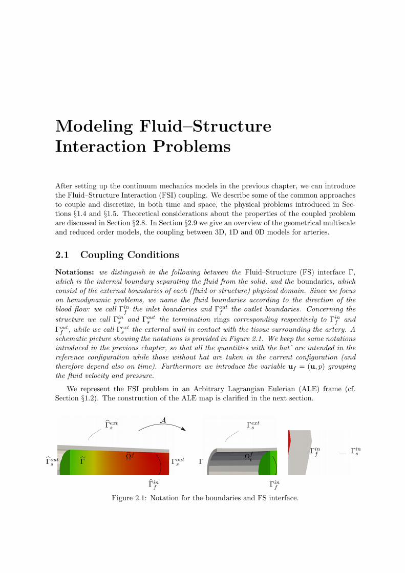
After setting up the continuum mechanics models in the previous chapter, we can introducethe Fluid–Structure Interaction (FSI) coupling. We describe some of the common approachesto couple and discretize, in both time and space, the physical problems introduced in Sec-tions §1.4 and §1.5. Theoretical considerations about the properties of the coupled problemare discussed in Section §2.8. In Section §2.9 we give an overview of the geometrical multiscaleand reduced order models, the coupling between 3D, 1D and 0D models for arteries.
2.1 Coupling Conditions
Notations: we distinguish in the following between the Fluid–Structure (FS) interface Γ,which is the internal boundary separating the fluid from the solid, and the boundaries, whichconsist of the external boundaries of each (fluid or structure) physical domain. Since we focuson hemodynamic problems, we name the fluid boundaries according to the direction of theblood flow: we call Γinf the inlet boundaries and Γoutf the outlet boundaries. Concerning thestructure we call Γins and Γouts the termination rings corresponding respectively to Γinf andΓoutf , while we call Γexts the external wall in contact with the tissue surrounding the artery. Aschematic picture showing the notations is provided in Figure 2.1. We keep the same notationsintroduced in the previous chapter, so that all the quantities with the hatˆare intended in thereference configuration while those without hat are taken in the current configuration (andtherefore depend also on time). Furthermore we introduce the variable uf = (u, p) groupingthe fluid velocity and pressure.
We represent the FSI problem in an Arbitrary Lagrangian Eulerian (ALE) frame (cf.Section §1.2). The construction of the ALE map is clarified in the next section.
Γouts ΓΩf
Γinf
ΓextsA
Γouts ΓΩft
Γexts
Γinf
ΓinsΓinf
Figure 2.1: Notation for the boundaries and FS interface.
CHAPTER 2. MODELING FLUID–STRUCTURE INTERACTION PROBLEMS
On the FS interface Γ the coupling is expressed through:
• the continuity of the velocity;
• the continuity of the stresses;
• the continuity of the domain displacement (geometric adherence).
The last coupling condition is at a certain extent artificial, since it is introduced by the ALEformulation of the fluid equation. It expresses the constraint on the fluid domain to follow thematerial particles of the solid on the interface Γ. The system of equations with the couplingconditions reads:
ρf∂u∂t
∣∣∣∣ex −∇x·σf + ρf (u−w) · ∇xu = ff in Ωft
∇x·u = 0 in Ωft
ρs∂2ds∂t2
−∇bx·Π = fs in Ωs
∂ds∂t
= u At on Γ (2.1.1)
σf nf + Πns = 0 on Γ (2.1.2)
∂df∂t
= w At on Γ, (2.1.3)
where often the body forces ff and fs are set to zero in hemodynamic applications (theycould account e.g. for the gravity force). We recall that from the Piola transform (1.1.10) wehave σf = JF−1σf . The last three equations (2.1.1), (2.1.2), and (2.1.3) represent the threecoupling conditions. The last one, as anticipated, is the geometric adherence constraint onthe ALE map stating that the fluid domain must follow the material FS interface.
2.2 Three Fields Formulation
At every time t > 0 the coupled FSI problem can be refounded as being made of three coupledsub-problems. A fluid problem
F(uf , ds, df ) = 0, (2.2.1)
describing the physics of the fluid through the equations introduced in Section §1.4. Thisproblem consists in finding the fluid velocity and pressure uf = (u, p) 3 given the solid dis-placement ds (or traction vector Πns, or a combination of both) and the domain displacementdf . We do not bind the notation for the fluid problem F to a specific interface condition,neither to a specific form (conservative or not) of the momentum conservation equation.When needed we distinguish the cases of Dirichlet, Neumann, or Robin coupling conditionsby calling the fluid problem FD, FN , or FR respectively.
A solid problemS(uf , ds) = 0, (2.2.2)
3to light the notation in the following pages we group the fluid velocity and pressure fields
26

2.2. THREE FIELDS FORMULATION
representing the structure equation introduced in Section §1.5. This problem consists infinding the solid displacement ds given the fluid velocity u (or traction vector σfnf , or acombination of both). The solid problem, as the fluid one, is not bound to a specific interfacecondition (which anyway has to be different from the one chosen for the fluid problem, in orderfor the coupled problem to be properly defined). Also in this case we distinguish the threepossible coupling conditions, Dirichlet, Neumann and Robin, with appropriate notations, SD,SN and SR respectively.
A geometry problem
G(ds, df ) = 0, (2.2.3)
defining the ALE map At, and thus the fluid computational domain. This problem is coupledto the solid problem through the geometric adherence condition (2.1.3), that we can writeequivalently as
df = ds on Γ. (2.2.4)
The arbitrariness of the ALE approach also reflects in the arbitrary choice of the geometryproblem. Our choice, which is quite common in this context, consists in describing the fluiddomain displacement df as a harmonic extension of the solid displacement ds|bΓ from the FSinterface Γ to the interior of the fluid reference domain Ωf ⊂ R3:
−∆df = 0 in Ωf
df = ds on Γ,∇bxdf · nf = 0 on ∂Ωf \ Γ,
(2.2.5)
The ALE mapping is then defined as
At : Ωf → Ωft
x 7→ At(x) = x+ df (x),
so that the current domain Ωft is defined as Ωf
t = At(Ωf ).In literature many other approaches to update the mesh displacement have been proposed
(see e.g. [DGH82, STB03]). The goal of these methods is to be computationally cheap andto keep bounded the mesh elements aspect ratio even under large displacements.
In this work we frequently group the fluid and geometry problems, in which case we notethe Fluid–Geometry problem FG:
FG(uf , ds) = 0.
Notations: we call ΓfD and ΓsD the Dirichlet boundaries (without the interface Γ) ofΩft and Ωs respectively, while the Neumann boundaries are noted ΓfN and ΓsN . Furthermore
the Dirichlet boundary of Ωf with respect to the mesh motion equation (2.2.5), which is thefluid boundary where the domain motion is prescribed (e.g. when a portion of the fluid domainboundary is fixed), will be noted ΓfF ixed. The conditions imposed on the boundaries are problemdependent. We denote with gDf : ΓfD → R3, gDs : ΓsD → R3, gDm : ΓfF ixed → R3 the Dirichlet
boundary data for the fluid, solid and geometry problems respectively, while gNf : ΓfN → R3 andgNs ∈ ΓsN → R3 represent the Neumann boundary data for the fluid and the solid problems.
27

CHAPTER 2. MODELING FLUID–STRUCTURE INTERACTION PROBLEMS
2.3 Time Discretization for the Structure Problem
The structure model is described by a PDE which is second order in time. Suitable andpopular methods available in literature for the time discretization of such problem are themid point scheme, Newmark (see [Nob01, Ch.4.8]) or the generalized-α scheme [RSFW09,DP07, BCHZ08]. The latter is a generalization of the Newmark scheme, while the mid pointscheme can be viewed as a Newmark scheme with a particular choice of the coefficients[Nob01, Ch.4.8]. We report here the mid point scheme for a generic second-order ODE whichcan represent e.g. the momentum conservation for the solid problem (1.5.4)
M
(∂2ds∂t2
,∂ds∂t
, ds
)= 0. (2.3.1)
The mid point scheme readsdn+1s − dnsδt
=˙dn+1s + ˙dns
2
M
( ˙dn+1s − ˙dnsδt
,˙dn+1s + ˙dns
2,dn+1s + dns
2
)= 0
(2.3.2)
These are two equations in the unknowns dn+1s and ˙dn+1
s to be solved at each time step.We report below a discretization of (2.3.1) with the generalized-α method:
0 = M(¨dn+αms ,
˙dn+αfs , dn+αf
s )
dn+αfs = dns + αf (dn+1
s − dns )˙dn+αfs = ˙dns + αf ( ˙dn+1
s − ˙dns )¨dn+αfs = ¨dns + αm(¨dn+1
s − ¨dns )
dn+1s = dns + δt
˙dns +(δt)2
2
[(1− 2β)¨dns + 2β ¨dn+1
s
](2.3.3)
˙dn+1s = ˙dns + δt[(1− γ)¨dns + γ
¨dn+1s ], (2.3.4)
where αf , αm, β, γ, are arbitrary real parameters defining the method, while δt is the time
step. It is a system of 6 equations in the unknowns dn+1s ,
˙dn+1s , ¨dn+1
s , dn+αfs ,
˙dn+αfs , ¨dn+αf
s .With αf = αm = 1 we have the Newmark scheme, and if also γ = 1
2 and β = 14 we obtain the
mid point scheme.
Remark 2.3.1. To obtain the mid point scheme from the generalized-α it is sufficient tosubstitute the coefficients αf , αm, β, and γ in (2.3.4)
δt
[12
¨dns +12
¨dn+1s
]= ˙dn+1
s − ˙dns ,
then substituting in (2.3.3) we obtain directly
dn+1s − dnsδt
=˙dn+1s + ˙dns
2,
which is the first equation in (2.3.2).
28

2.4. TIME DISCRETIZATION FOR THE FLUID–GEOMETRY PROBLEM
Chung and Hulbert [CH93] showed that second order accuracy is attained if
γ =12− αf + αm,
andβ =
14
(1− αf + αm)2.
The scheme is unconditionally stable if αm ≥ αf ≥ 12 . Furthermore in [CH93] optimal choices
for the parameters αf and αm are retrieved:
αcm =2− ρ∞1 + ρ∞
,
αcf =1
1 + ρ∞,
where the parameter ρ∞ is the limit spectral radius of the amplification matrix for infinitetime steps. If ρ∞ = 1 then αf = αm = 1
2 and there is no damping of the high frequencycomponents.
A similar set of coefficients was devised by Jansen et al. in [JWH00] for the first orderequations. We report for completeness the corresponding values of αf and αm in this case
αcm =12
3− ρ∞1 + ρ∞
,
αcf =1
1 + ρ∞.
Notice that in [DP07, BCHZ08] the generalized-α scheme is used for both the fluid andstructure fields.
Also the structure equation can be nonlinear, the only nonlinearity coming from theconstitutive law relating the stress and the strain tensors. As in the fluid–geometry casethere is the option of considering part (or all) of the nonlinear term explicitly, or to linearizeusing Newton or fixed-point. The discussion about the last two strategies is reported in thenext chapter.
The time advancing scheme used in Part III for the numerical simulations is the mid pointrule (2.3.2).
2.4 Time Discretization for the Fluid–Geometry Problem
A large variety of time discretizations of the incompressible Navier–Stokes equations on mov-ing domains can be found in literature, depending on the targeted application. However usingthe ALE formulation imposes some constraints. In fact the choice of the time discretizationof the convective term (β · ∇x)u plays a fundamental role in determining the order of thetime advancing scheme and its stability properties (through the Geometric Conservation Law,cf. Section §2.8). For instance one may chose a time advancing scheme of second order andobtain only a first order approximation in time, see e.g. [FvdZG06]. The stability issue isdiscussed more in detail in Section §2.8, while here we just describe some of the possiblechoices adopted in literature.
29

CHAPTER 2. MODELING FLUID–STRUCTURE INTERACTION PROBLEMS
The approaches more frequently used in hemodynamics are one-step implicit methodslike the implicit Euler scheme (first order accurate), the generalized alpha scheme (first orsecond order accurate), Crank–Nicholson (second order accurate) or sometimes multistepBDF schemes (see [QSS00]).
The implicit Euler scheme consists in considering all the quantities at the current timestep. For instance the discretization of the generic non conservative form of an ALE fieldreported in equation (1.3.9), i.e.,
∂α
∂t
∣∣∣∣ex = ∇x·(Θ−α⊗ u) + (w · ∇x)α+ b,
reads:αn+1
δt−∇x·(Θn+1 −αn+1 ⊗ un+1)−w?∇xαn+1 =
αn
δt+ bn+1, (2.4.1)
where α and Θ are a vectorial and tensorial quantities introduced in (1.3.9).The approximation of the domain velocity w? is independent of the time approximation
chosen for the equation, indeed it defines how the coupling between the problems F and Gis handled. If these two problems are not strongly coupled the approximation of the fluiddomain velocity w? affects the order of the time discretization.
The generalized-α scheme was first introduced for structural dynamic applications in [CH93]for second order ODEs. It was then adapted to first order ODEs in [JWH00]. In FSIcontext the generalized-α has been used e.g. in [DP07, BCHZ08]. The Crank–Nicholsonscheme applied to the fluid problem in FSI has been used in e.g. [HT06, Nob01], whilein [RSFW09, FvdZG06] the BDF2 scheme is used. All these choices can lead to a globallysecond order in time FSI scheme, when the structure solver and coupling conditions are alsosecond order accurate. The first order time discretizations (e.g. implicit Euler) for the FGproblem are more common, however we anticipate that using the conservative formulationof the momentum equation, implicit Euler time discretization and choosing w? = wn+1 animportant condition (the DGCL condition, cf. Section §2.8) is not fulfilled, which can lead tothe instability of the scheme [Nob01, Ch.4.7].
We remark also that the applications can dictate constraints on the timestep (e.g. whensimulating turbulent fluids through DNS), in these cases an explicit time discretization canbe employed for the fluid problem (see e.g. [BA09, FL00]).
With the aim of keeping a general notation that applies to every time discretization, aswell as to every form of the conservation equations and interface conditions, in what followswe denote the time-discretized fluid and solid problems by Fn and Sn respectively.
The coupled fluid–structure problem has several levels of nonlinearities, some of thembeing related to the fact that we chose to write the equations in ALE form:
• the convective term of the Navier–Stokes equations in fixed domains
(u · ∇x)u; (2.4.2)
• the advection term introduced by the ALE formulation
(w · ∇x)u; (2.4.3)
30
2.4. TIME DISCRETIZATION FOR THE FLUID–GEOMETRY PROBLEM
• the dependence of the fluid domain displacement df on the displacement of the struc-ture.
At every time step they can be solved by using a Newton or fixed point algorithm, as it isdiscussed in the next chapter. By properly choosing the time discretization the FSI problemat each time step may result to be linear.
We call Fully Implicit (FI) time discretization (see e.g. [BCHZ08, TSS06, HHB08, KGF+09,BC10a, DP07, Hro01, MNS06, GV03, LM01, KW08b]) the implicit treatment of all the non-linearities introduced above as well as of the coupling with the solid problem. It leads ingeneral to a more accurate and robust time discretization, but it is also the most expensiveapproach among those discussed here, since the solution of the nonlinearities needs extracomputational efforts.
Different approaches can be obtained by modifying the way the nonlinear terms are dis-cretized in the FI approach. For instance being n + 1 the current time step, the nonlinear-ity (2.4.2) can be discretized in time, given an extrapolation u? of the fluid velocity from theprevious time steps, in the following way
(u? · ∇x)un+1. (2.4.4)
With this choice the term (2.4.4) becomes linear. This is a suitable choice when the char-acteristic Reynolds number of the fluid flow is not very high, and thus the nonlinearity ofthe convective term is not predominant (condition usually fulfilled in hemodynamics). Thesimplest approximation corresponds to choosing u? = un. It introduces an error of thefirst order in time and can be easily modified if a time advancing scheme of higher or-der is used. This approximation for the convective term of the fluid problem is used e.g.in [FM05, DDFQ06, Nob01, BQQ08b, Dep04].
Also the nonlinearity (2.4.3) can be discretized in time as
(w? · ∇x)un+1, (2.4.5)
where w? is an explicit extrapolation of the fluid domain velocity. Together with the term (2.4.4)it leads to a linearized convective term [CDFQ11].
The nonlinearity due to the moving domain is the most difficult to handle implicitly (cf.Chapter 3). Considering the fluid domain at the previous time step is a suitable approximationwhen the displacements are not very large. Its explicit treatment, combined with (2.4.4)and (2.4.5), leads to the Geometry–Convective Explicit (GCE) time discretization (see e.g.[CDFQ11, BQQ08a]), in which the fluid problem is linear. In Tezduyar et al., see e.g. [TSS06],some different coupling strategies are also investigated. In particular the quasi–direct couplingin their convention corresponds to a fully coupled scheme where the geometry is consideredexplicitly, while the direct coupling corresponds to the fully implicit discretization introducedabove.
Besides the time discretization of the nonlinear terms, frequently the methods differ withrespect to the time discretization of the coupling between fluid and structure. However, sincethis subject has been extensively studied and since it is critical for the stability of the method,we chose to leave it for Section §2.8, where the stability issue is addressed.
31
CHAPTER 2. MODELING FLUID–STRUCTURE INTERACTION PROBLEMS
2.5 Fully Implicit and Convective Explicit Schemes
Using the fully implicit approach for the fluid–geometry problem, the coupled time-discretesystem of equations at the time level t = tn+1 reads
Fn(ufn+1, dn+1s , dn+1
f ) = 0
Sn(ufn+1, dn+1s ) = 0 (2.5.1)
Gn(dn+1s , dn+1
f ) = 0
We denote the first order discrete time derivative for the fluid problem as δt, while thediscretization of the second derivative in time of the structure equation is represented by δtt.The whole system of equations in strong form, considering the fluid momentum conservationequation in non-conservative form, reads
ρfδtun+1 + ρf((un+1 −wn+1) · ∇x
)un+1 −∇x·σfn+1 − ffn+1 = 0 in Ωf
t n+1
∇x·un+1 = 0 in Ωft n+1
ρsδttdn+1s −∇bx·σn+1
o s − fsn+1 = 0 in Ωs
−∆dn+1f = 0 in Ωf (2.5.2)
Πn+1ns + σn+1f · nf = 0 on Γ
un+1 Atn+1 − δtdn+1s = 0 on Γ
dn+1f − dn+1
s = 0 on Γ
+conditions on the external boundaries.
The solution of the geometry problem defines the ALE map Atn+1 and the fluid domain attime tn+1, Ωf
t n+1 = Atn+1(Ωf ). Given (at least) dn+1f and dnf the fluid domain velocity can
be computed aswn+1 = δtdn+1
f A−1tn+1
. (2.5.3)
When the convective term in the fluid momentum equation is discretized using both (2.4.4)and (2.4.5), while the fluid geometry is still considered implicitly, we call the correspondingtime discretization of the fluid–geometry problem Convective Explicit (CE).
2.6 Geometry–Convective Explicit Scheme
In the Geometry–Convective Explicit (GCE) time discretization the nonlinear term (2.4.3) islinearized using (2.4.5) and the coupling of the fluid and the geometry problems is explicit.The GCE counterpart of (2.5.1) reads
Fn(ufn+1, dn+1s , dn+1
f ) = 0
Sn(ufn+1, dn+1s ) = 0 (2.6.1)
Gn(dns , dn+1f ) = 0.
Although the convective term is linearized using an explicit extrapolation of the fluid velocityu?, with an abuse of notation we use the same symbol for the fluid problem Fn as in the fullyimplicit case.
32
2.7. SPACE DISCRETIZATION
We write explicitly below the time discretized equations in strong form defining the GCEscheme. The geometry equation,
Gn(dns , dn+1f ) = 0,
is solved separately once per time step and the fluid domain velocity wn+1 is computedusing (2.5.3).
The time discrete fluid–structure problem reads (the fluid momentum equation beingwritten in non-conservative form):
ρfδtun+1 + ρf((un −wn+1
)· ∇x)un+1 −∇x·σfn+1 = ffn+1 in Ωf
t n+1, (2.6.2)
∇bx·un+1 = 0 in Ωft n+1,
ρsδttdn+1s −∇bx·(Π)n+1 = fsn+1 in Ωs,
un+1 Atn+1 − δtdn+1s = 0 on Γ,
Πn+1ns + (σf )n+1 · nf = 0 on Γ,+conditions on the external boundaries.
As already mentioned this problem has the advantage of being linear when the structureequation is linear, at any given time step. In applications, as shown in Sections §5.4 and §6.2,this time discretization also leads to a stable and robust FSI solver and can be efficientlyimplemented in parallel.
2.7 Space Discretization
In this section we write the weak form and describe the space finite elements discretizationof the FSI system. We refer to [LM01, Nob01] for details.
Recalling the notations introduced in Section §2.2 we can define the following functionalspaces
Uf = v = v At−1|v ∈ H1(Ωf )3,
Up = q = q At−1|q ∈ L2(Ωf ),
U s = H1(Ωs)3,
Ug = H1(Ωf )3,
UbΓ = H1/2(Γ)3,
V f = v = v At−1|v ∈ H1(Ωf )3, v = 0 on ΓfD,
V s = v ∈ H1(Ωs)3| v = 0 on ΓsD,
V g = v ∈ H1(Ωf )3|v = 0 on ΓfF ixed.
If Ωft and Ωf are bounded and with Lipschitz continuous boundary, At ∈W 1,∞(Ωf )3 and
At−1 ∈ W 1,∞(Ωft )3, then Uf ≡ H1(Ωf
t )3. Furthermore, if also A ∈ H1(T ⊂ R;W 1,∞(Ωf )3)holds, then, for u ∈ H1(T ;H1(Ωf )3), u = u A−1 ∈ H1(T ;Uf ) ≡ H1(T ;H1(Ωf
t )3) [Nob01,Ch.1.3].
We report hereafter the weak formulation of the FSI system in non-conservative andconservative form. We first introduce the way in which the stress continuity coupling condition
33
CHAPTER 2. MODELING FLUID–STRUCTURE INTERACTION PROBLEMS
is enforced (in a weak sense), and show that enforcing this coupling condition amounts tochoosing matching test functions across the interface.
While the velocity continuity coupling condition is usually imposed in its strong form, thecontinuity of stresses through the interface can be imposed in a weak way by equating thevariational residuals of the two momentum conservation equations restricted to the interface.In fact if we write the variational formulation of the fluid momentum equation, consideringan arbitrary vf ∈ V f , we have∫
Ωft
(ρf∂u∂t
∣∣∣∣ex · vf + (ρf (u−w) · ∇x)u · vf + σf : ∇xvf − ff · vf)
dΩtf+
−∫
ΓfN
gNf · trΓ (vf ) dγ =∫
Γσfnf · trΓ (vf ) dγ. (2.7.1)
The same can be done for the structure equation for vs ∈ V s, leading to∫bΩs(ρs∂2ds∂t2
· vs − (∇bx·Π)vs − fsvs
)dΩ
s−∫
ΓsN
gNs · trbΓ (vs) dγ =∫
bΓ Πns · trbΓ (vs) dγ.
(2.7.2)We introduce now the two linear continuous lift operators
Lf : UbΓ → V f ,
Ls : UbΓ → V s.
Expressing the stress tensors in the reference configuration, we can write the stress con-tinuity equation on the interface in a weak form,∫
bΓ Πns · ψ dγ +∫
bΓ σf nf · ψ dγ = 0 ∀ψ ∈ U bΓ, (2.7.3)
as ∫bΩs(ρs∂2ds∂t2
· Ls(ψ))dΩ +
∫bΩs (Π : ∇bxLs(ψ)− fs · Ls(ψ)) dΩ−
∫ΓsN
gNs · Ls(ψ) dγ
+∫
bΩf(ρf∂u At−1
∂t
∣∣∣∣ex · Lf (ψ) + ρf((u At−1 −w At−1) · ∇bx)u At−1 · Lf (ψ)+
+σf : ∇bx·Lf (ψ)− ff · Lf (ψ))dΩ−
∫ΓfN
gNf · Lf (ψ) dγ = 0 ∀ψ ∈ U bΓ. (2.7.4)
Thus the weak imposition of the stress continuity can be achieved by simply choosing testfunctions vf ∈ V f and vs ∈ V s which are matching on the FS interface. The weak impositionof the stresses leads sometimes to more stable numerical results [FLT98, LM01].
Following [LM01] and [Nob01] we consider a global weak formulation of the FSI problem.To this end we define the space W = (vf ,vs) ∈ V f ×V s|trbΓ (vf At) = trbΓ (vs). Imposingthe weak stress continuity coupling condition, as previously stated, is obtained automaticallyby choosing the test functions in this space, i.e, supposing that the test functions restrictedto the interface are matching.
34

2.7. SPACE DISCRETIZATION
We recall the notation for the Dirichlet boundary data for the three problems: gDf : ΓfD →R2, gDs : ΓsD → R2, gDm : ΓfF ixed → R2. The weak form of the equations (1.4.6), (1.4.2), (1.5.4)and (2.2.5) reads: for almost every t ∈ T find u : T → Uf such that t 7→ u(t) and u = gDf on
ΓfD , p : T → Up such that t 7→ p(t) , ds : T → U s such that t 7→ ds(t) and ds = gDs on ΓsD,df : T → Ug such that t 7→ df (t) and df = gDm on ΓfF ixed satisfying∫
Ωft
ρf∂u∂t
∣∣∣∣ex · vf + (ρf (u−w) · ∇x)u · vf + σf : ∇xvf dΩtf+
+∫
bΩs ρs∂2ds∂t2
· vs + Π : ∇xvs dΩs
=∫
bΩs fs · vs dΩs−∫
ΓsN
gNs · vs dγ+
+∫
Ωft
ff · vf dΩtf −
∫ΓfN
gNf · vf dγ, ∀(vf ,vs) ∈W,
(2.7.5)∫Ωft
u · ∇xq dΩtf = 0 ∀q ∈ Up,∫
bΩf ∇bxdf : ∇bxvm dΩf
= 0 ∀vm ∈ V g.
u At =∂ds∂t
on Γ
df = ds on Γ.
To write the conservative form it is sufficient to replace the fluid momentum contributionin (2.7.5) with
Dt
∫Ωft
ρfu · vf dΩt +∫
Ωft
[(σf − ρfu⊗ β) : ∇xvf − ff · vf ] dΩtf −
∫ΓfN
σfnf · vf dγ = 0.
(2.7.6)The Dirichlet boundary conditions are usually enforced strongly, i.e., discretizing directly
equation (2.1.1), while the Neumann boundary conditions are usually imposed weakly, i.e.,given the boundary data gNf ∈ (H
12 (ΓfN ))3 and gNs ∈ (H
12 (ΓsN ))3 enforcing the Neumann
boundary conditions is obtained by substituting the boundary terms in (2.7.5).
Remark 2.7.1. If the geometric adherence coupling condition holds, then, on the FS in-terface, the ALE map equals the deformation map φt, and the fluid domain velocity equalsthe fluid velocity w = u. Since the description of the boundary for both the fluid and solidproblems is Lagrangian no interpolation is required when enforcing the coupling (if the finiteelements are conforming across the interface).
Remark 2.7.2. The test functions in V f are piecewise constant in time, so that
∂vf∂t
∣∣∣∣ex = 0 ∀vf ∈ V f . (2.7.7)
Due to (2.7.7) the test functions vf can always be taken out of the ALE derivatives. Inparticular this implies the following equality
Dt
∫Ωft
u · vf dΩtf =
∫Ωft
∂u∂t
∣∣∣∣ex · vf + u(∇x·w) · vf dΩtf . (2.7.8)
35
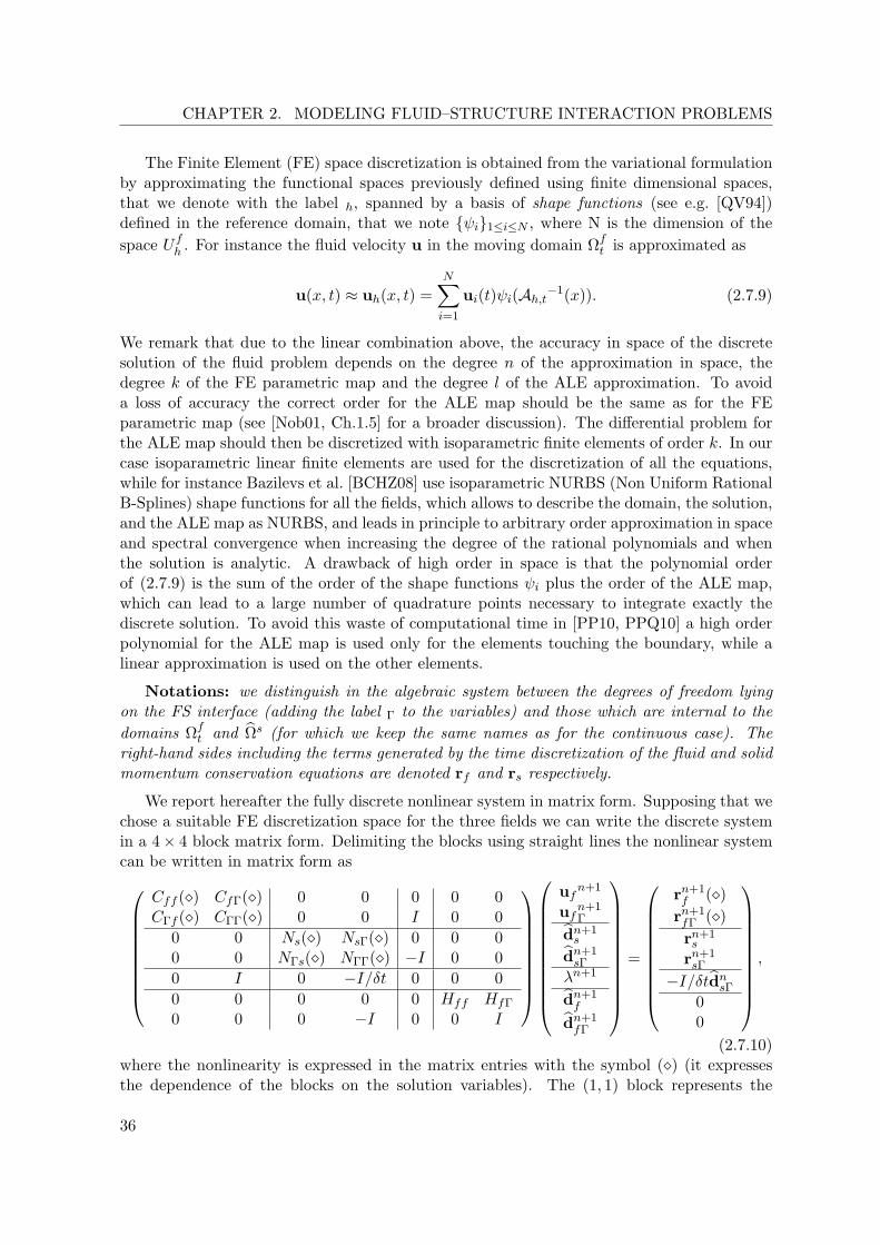
CHAPTER 2. MODELING FLUID–STRUCTURE INTERACTION PROBLEMS
The Finite Element (FE) space discretization is obtained from the variational formulationby approximating the functional spaces previously defined using finite dimensional spaces,that we denote with the label h, spanned by a basis of shape functions (see e.g. [QV94])defined in the reference domain, that we note ψi1≤i≤N , where N is the dimension of thespace Ufh . For instance the fluid velocity u in the moving domain Ωf
t is approximated as
u(x, t) ≈ uh(x, t) =N∑i=1
ui(t)ψi(Ah,t−1(x)). (2.7.9)
We remark that due to the linear combination above, the accuracy in space of the discretesolution of the fluid problem depends on the degree n of the approximation in space, thedegree k of the FE parametric map and the degree l of the ALE approximation. To avoida loss of accuracy the correct order for the ALE map should be the same as for the FEparametric map (see [Nob01, Ch.1.5] for a broader discussion). The differential problem forthe ALE map should then be discretized with isoparametric finite elements of order k. In ourcase isoparametric linear finite elements are used for the discretization of all the equations,while for instance Bazilevs et al. [BCHZ08] use isoparametric NURBS (Non Uniform RationalB-Splines) shape functions for all the fields, which allows to describe the domain, the solution,and the ALE map as NURBS, and leads in principle to arbitrary order approximation in spaceand spectral convergence when increasing the degree of the rational polynomials and whenthe solution is analytic. A drawback of high order in space is that the polynomial orderof (2.7.9) is the sum of the order of the shape functions ψi plus the order of the ALE map,which can lead to a large number of quadrature points necessary to integrate exactly thediscrete solution. To avoid this waste of computational time in [PP10, PPQ10] a high orderpolynomial for the ALE map is used only for the elements touching the boundary, while alinear approximation is used on the other elements.
Notations: we distinguish in the algebraic system between the degrees of freedom lyingon the FS interface (adding the label Γ to the variables) and those which are internal to thedomains Ωf
t and Ωs (for which we keep the same names as for the continuous case). Theright-hand sides including the terms generated by the time discretization of the fluid and solidmomentum conservation equations are denoted rf and rs respectively.
We report hereafter the fully discrete nonlinear system in matrix form. Supposing that wechose a suitable FE discretization space for the three fields we can write the discrete systemin a 4× 4 block matrix form. Delimiting the blocks using straight lines the nonlinear systemcan be written in matrix form as
Cff () CfΓ() 0 0 0 0 0CΓf () CΓΓ() 0 0 I 0 0
0 0 Ns() NsΓ() 0 0 00 0 NΓs() NΓΓ() −I 0 00 I 0 −I/δt 0 0 00 0 0 0 0 Hff HfΓ
0 0 0 −I 0 0 I
ufn+1
ufn+1Γ
dn+1s
dn+1sΓ
λn+1
dn+1f
dn+1fΓ
=
rn+1f ()
rn+1fΓ ()rn+1s
rn+1sΓ
−I/δtdnsΓ00
,
(2.7.10)where the nonlinearity is expressed in the matrix entries with the symbol () (it expressesthe dependence of the blocks on the solution variables). The (1, 1) block represents the
36

2.7. SPACE DISCRETIZATION
discrete fluid problem equations, the block (2, 2) represents the discrete solid problem, whileblock (4, 4) represents the discretization of the geometry problem. The off-diagonal entriesenforce the coupling conditions between the three fields. In this discrete formulation we havesupposed a first order time discretization of the velocity continuity coupling condition. Theright hand sides rn+1
f and rn+1s are composed by the volume forces and the terms of the
time discretization which depend on the previous time steps. The multiplier λ is introducedto enforce the coupling conditions across the FS interface. When the coupling is enforcedintroducing a new variable we say that the linear system is written in augmented form. Infact from (2.7.4) we can write the weak stress continuity as
CΓfuf + CΓΓuf +NΓsds +NΓΓdsΓ = 0.
We can rewrite the previous equation as
CΓfuf + CΓΓuf = λ, (2.7.11)
NΓsds +NΓΓdsΓ + λ = 0.
Thus the third block-column of the matrix in (2.7.10) enforces the stress continuity coupling,while the third block-row represents the velocity continuity.
Note that we defined the multiplier λ at the algebraic level, which means that it consistsof a vector with the dimension of the degrees of freedom sitting on the FS interface. Howeverdue to (2.7.11) it can be interpreted as the FE discretization of the integral of the surfacetraction on the interface:
∫Γ σfn
f dγ.
The weak form of the GCE system discretized in space leads to the following linear systems:the mesh motion equation can be solved separately because in the geometry–explicit timediscretization the fluid domain and the mesh velocity are extrapolated from the interfacedisplacement of the previous time step. We have(
Hff HfΓ
0 I
)(dn+1f
dn+1fΓ
)=(
0dnsΓ
).
The new domain Ωft at time tn+1 is then recovered by means of the nodes of the mesh
following dn+1f . The integrals relative to the FE discretization of the fluid are computed with
respect to the new mesh, yielding the following linear system:Cff CfΓ 0 0 0CΓf CΓΓ 0 0 I
0 0 Ns NsΓ 00 0 NΓs NΓΓ −I0 I 0 −I/δt 0
ufn+1
ufn+1Γ
dn+1s
dn+1sΓ
λn+1
=
rn+1f
rn+1fΓ
rn+1s
rn+1sΓ
−I/δtdnsΓ
. (2.7.12)
Since the GCE problem is linear, the symbol () is removed from the blocks in (2.7.10).
The general Jacobian system for CE or FI is reported in the next chapter, while the parallelsolution and preconditioning of the various Jacobian systems is addressed in Chapter 4 inwhich the blocks structure of the matrix is exploited.
Notations: in the following chapters we distinguish between three Jacobian matricescoming from three different choices for the time discretization: we call JFI the Jacobian
37

CHAPTER 2. MODELING FLUID–STRUCTURE INTERACTION PROBLEMS
matrix of the system (2.7.10), JCE the Jacobian of (2.7.10) when the convective term islinearized using (2.4.4) and (2.4.5) (but considering implicitly the geometric nonlinearity)and JGCE the matrix in (2.7.12).
2.7.1 Interior Penalty Stabilization
For our simulations we discretize the Navier–Stokes equations by P1–P1 elements stabilizedby interior penalty (IP) [BF07, BFH04, PB05].
The IP stabilization consists of adding to the Galerkin discrete formulation of the fluidproblem some consistent terms that penalize the jumps of given quantities across the bound-ary Γe of each element. We denote with J·K the jumps across the element boundaries; thepenalization terms added to the fluid momentum equation are the following, for vf ∈ V f :
• jβ(u,vf ) =∫
Γeγβ
h2
‖u−w‖L∞J(u−w) · ∇xuKJ(u−w) · ∇xvf K dγ, where γβ is a constant
to be chosen. This term penalizes the jump of the convective term across the interfaceof the finite elements, and it is used to stabilize convection dominated flows.
• jdiv(u,vf ) =∫
Γeγdivh
2‖u−w‖L∞J∇xuKJ∇xvf K dγ, where γdiv is a constant. This termpenalizes the jumps of the velocity gradient.
Another term to stabilize the pressure is added to the continuity equation in weak form.This penalization term allows to circumvent the inf–sup condition and to use equal orderfinite elements for velocity and pressure fields. For q ∈ Up, and a constant parameter γp,
jp(p, q) =∫
Γe
γph3
maxh‖u−w‖L∞ , µfJ∇xpKJ∇xqK dγ.
This term penalizes the jump of the pressure gradient across the elements and may lead toan inconsistency when the exact solution features a discontinuous pressure gradient.
Note that although these terms are converging to zero with the grid size h, and they areidentically null in the continuous case, they are in general different from zero when discretizedin space. This implies in particular that the discrete continuity equation is not satisfiedexactly.
2.8 Analysis of the Coupled Problem
In this section we report results about the well posedness of the FSI problem and we discuss thestability of some of the different time discretization schemes introduced above. We introducethe concept of geometric conservation laws and the associated conditions for a numericalscheme. To conclude the section the stability of the coupling between the fluid–geometry andstructure problems is investigated.
2.8.1 Analysis of Simplified Coupled Models
We refer in this section mainly to Y. Maday [FQV09, Ch.8], where it is reported an overviewof recent results and methodologies to prove the well posedness of the FSI system.
In the usual definitions of stability, a system is stable when its energy is bounded by aconstant which depends on the forcing terms and on the boundary conditions. A priori energyestimates are fundamental to prove the stability of a differential problem, just as they are
38

2.8. ANALYSIS OF THE COUPLED PROBLEM
important for the stability of a numerical method. A classical Faedo–Galerkin approach usede.g. in [Lio69] allows to prove the existence of a weak solution in the FSI context when thefluid domain motion is neglected and the structure is visco-elastic. The solution is proved tobe unique in the 2D case (see [Lio69, FQV09] for the proofs).
Starting from the variational formulation, the Faedo–Galerkin technique consists in defin-ing a sequence of finite dimensional test spaces converging to the original infinite dimensionalspace. Then the existence and uniqueness of the solution for the finite dimensional problemsis proved. Thanks to proper a priori estimates for all the terms in the variational formulation,there exists a subsequence for each term which converges weakly in the infinite dimensionalspace. For the FSI case considered in [Lio69] a compactness theorem is needed for the non-linear convective term to pass to the limit.
An analysis by Chambolle et al. [CDEG05, FQV09] generalizes the previous strategy toFSI with moving fluid domain. The fact that the domain motion depends on the solutionadds a nonlinearity which is a major complication for the analysis. In that work the solid ismodeled as a visco-elastic plate. We give here an idea of the method used for the analysis.
Definition 2.8.1 (Compact operator). Let X and Y be two Banach spaces, and T : X → Yan operator. T is compact iff
• it is continuous;
• it maps bounded sets into relatively compact sets.
The Schauder Fixed point theorem which can be found e.g. in [Zei91], is used to completethe proof of the existence.
Theorem 2.8.1 (Schauder Fixed-Point theorem). Let M be a nonempty, closed, bounded,convex subset of a Banach space X, and suppose that T : M → M is a compact operator.Then T has a fixed point.
This theorem is frequently used to prove the existence of solutions for nonlinear equationsin a Banach space. The proof of the existence of a weak solution for the FSI problem followsthe main steps listed below.
The fluid and solid problems are substituted by two regularized problems, such that thesolution is defined on a regularized current domain depending on a parameter ε.
The equations are linearized through fixed point, considering known the fluid domaindisplacement and the fluid velocity in the convective term. Given the solution (uo, dso), wecall S(uo, dso) the solution of the linearized system.
The linearized equations are recast back to the original configuration. A basis of eigen-functions for the Stokes problem is then used to generate a sequence of finite dimensional testspaces, and the Faedo–Galerkin technique is used, with steps analogous to those in [Lio69]recalled above. Using the a-priori estimates it is possible to conclude that the linearizedcontinuous problem has a unique solution.
Let us consider the image of the solver operator S of the linearized problem. Due tothe estimates and to classical theorems (Aubin’s lemma), this operator is relatively compact.Thus the Schauder’s theorem guarantees the existence of a fixed point for S (i.e., the solutionof the nonlinear regularized problem).
Eventually it is proved that the limit for ε → 0 converges to a solution of the originalproblem.
39
CHAPTER 2. MODELING FLUID–STRUCTURE INTERACTION PROBLEMS
Beirao da Veiga [BdV04, FQV09] provides a proof for the existence of a strong solution in2D, where the structure is modeled through a 1D generalized string model [FQV09, Ch.3.4].As in the previous analysis, the problem is formulated as a fixed point problem and theSchauder’s theorem is employed to show the existence. However the equations are writtenon an ALE reference domain, and the a priori estimates are performed there. The finalrequirements on the regularity of the solution in this case are more restrictive than in theprevious case.
Finally the existence of a strong solution for a 3D FSI problem is derived by Cheng et al.in [ACCS06]. The structure is modeled by a nonlinear Koiter shell model without the inertialterm. As in the previous work the analysis is performed in the reference configuration. In thisanalysis a uniqueness result is obtained under appropriate compatibility conditions betweeninitial and boundary data.
2.8.2 Stability and Geometric Conservation Law
The stability of the numerical schemes for FSI in ALE form is currently subject of research.As mentioned in Section §2.4 the unconditional stability on fixed domains does not implythat the same method used on moving domain is unconditionally stable as well. Usually toguarantee stability of a method it is necessary to find a bound for the energy of the discretizedsystem. This is achieved by means of a-priori error estimates (see [Nob01]). However thisapproach is not always possible (or easy), thus other types of stability can be devised [FGG01].
A well established condition that a discretization method should satisfy is the DiscreteGeometric Conservation Law (DGCL). A numerical scheme is said to satisfy the DGCL if it iscapable of reproducing constant (in space and time) solutions in the absence of forcing termsand with proper boundary conditions. This is not always true for problems in moving domainsadopting an ALE frame, and it depends on the time discretization chosen. The role of DGCLin the stability of numerical schemes for problems in moving domains was investigated in thelast years, in particular in Nobile [Nob01] it leads to an unconditional stability result for theimplicit Euler scheme, which will be recalled below, while in Farhat et al. [FGG01] DGCL insome cases is found to be equivalent to a discrete maximum principle.
The fulfillment of DGCL is automatic for any time discretization if the equations arewritten in non-conservative form. In fact, taking (2.7.1) and substituting a constant solutionwe obtain an identity independently of the time discretization employed.
On the other hand rewriting the conservative form (2.7.6) for a constant solution andwithout forcing term, we end up with the following equation
Dt
∫ωA
ρfu · vf dΩt =∫ωA
(ρfu · ∇xw) · vf dΩtf , (2.8.1)
which is the weak form of the Leibnitz transport formula (1.2.7) for a constant solution.Integrated in time it gives∫
ωAn+1
ρfu · vf dΩt −∫ωAn
ρfu · vf dΩt = INT tn+1
tn
[∫ωA
(ρfu · ∇xw) · vf dΩt
], (2.8.2)
where the term INT tn+1
tn denotes a chosen numerical integration in time from tn to tn+1.While condition (2.8.1) is referred to as Geometric Conservation Law (GCL) condition and
40

2.8. ANALYSIS OF THE COUPLED PROBLEM
it is a conservation equation, (2.8.2) is the discrete geometric conservation law and its formdepends on the choice of the time integrator.
Thus the DGCL condition consists in choosing a time integration scheme which allows tosatisfy exactly (1.2.7) for a constant solution. It can also be interpreted as a discretization ofJacobi’s formula(1.2.5): if DGCL holds then the discrete counterpart of (1.2.5) holds exactly.We see from this relation that the choice of the integration rule for the part of the convectiveterm related to the ALE description determines whether the scheme satisfies or not the DGCL.A different time integration can be chosen for the term u · ∇xw than for the other terms,leading to a scheme satisfying the DGCL. A rule to choose the time integration in order tosatisfy (2.8.1) consists in taking an integration scheme of order d ·s−1, where d is the numberof spatial dimensions and s is the polynomial order of the nodal displacement. A proof isgiven in [Nob01, Ch.1.8].
An a-priori error estimate for an FSI scheme, for which unconditional stability is proved,is derived in [Nob01, Ch.4.7]. The equations are discretized in time using an implicit Eulerscheme satisfying the DGCL (i.e., using a mid point scheme to discretize the fluid domainvelocity) for the fluid and BDF1 for the structure. A piecewise linear in time ALE map isused. In the energy estimates the DGCL comes into play when the term∫ tn+1
tn
∫Ωft
un+1h ∇x·w? dΩt
f
has to be bounded. In fact due to (2.8.2) (taking u as test function) the following equationholds:
INT tn+1
tn
∫Ωft
‖un+1h ‖2∇x·w? dΩt
f =∫
Ωftn+1‖un+1
h ‖2 dΩtf −
∫Ωft
n‖un+1
h ‖2 dΩtf . (2.8.3)
Substituting in the energy equation this identity allows to devise estimates which are indepen-dent of the mesh velocity w. Such results have not been found in case of the non-conservativeformulation, for which only conditional stability results have been proven.
In [FGG01] the importance of DGCL in the stability of numerical methods for nonlinearequations in moving domains is investigated. The analysis is applied to finite volumes schemes.The stability is defined in the sense of a discrete maximum principle, stating that there existtwo constants M and m such that the space average un of the numerical solution in a cell hasto satisfy m ≤ un ≤ M ∀n. The DGCL is shown to be necessary and sufficient condition inorder to satisfy this maximum principle in the case of theta-methods.
Also in [BG04] the influence of DGCL is addressed. The result found is that satisfy DGCLis neither necessary nor sufficient to guarantee the stability (in a sense specified in [BG04])of a numerical scheme. In fact a condition on the time step is derived for which an implicitEuler scheme that does not satisfy DGCL is stable. However also in [BG04] the importanceof using a scheme which satisfies DGCL is stressed, since e.g. the implicit Euler satisfyingDGCL is unconditionally stable, as discussed above.
In [LM01] it is also shown that not satisfying DGCL introduces for a conservative schemean error in the energy conservation which depends on the time discretization for the fluidemployed. Furthermore it is shown that using the non conservative formulation the errorintroduced in the energy balance is proportional to ∇x·β. Thus choosing ALE maps whichsatisfy ∇x·w = 0 can reduce the energy dissipation in non conservative schemes.
41

CHAPTER 2. MODELING FLUID–STRUCTURE INTERACTION PROBLEMS
2.8.3 Strong versus Weak Coupling
The choice of the time discretization introduces further distinctions among the methods.Besides the characterization of the methods as Fully Implicit, Geometry–Convective Explicit,etc., another classification concerns the way in which the coupling conditions are discretizedin time. We can devise three main classes of methods regarding the coupling strategies:
• Strongly (implicitly) coupled schemes. The coupling condition is enforced exactly ateach time-step (e.g. by means of an extra loop). As a result they can require a vari-able amount of coupling iterations, depending on the algorithm used and on physicalparameters [KW08b, MNS06, BNV08, BQQ08a].
• Fractional step (semi-implicit coupling) schemes4. They involve a splitting of the systemin two problems, a solution of both and a successive correction of the fluid velocity.These schemes require in general a time step restriction to converge [FGG07, ACF09,QQ07, BQQ08b].
• Weakly (explicitly) coupled, or staggered, schemes. These methods are very cheap sincethey require just one solution of each subproblem per time step. In some cases theyare proved to be unconditionally unstable (due to the added mass effect, as explainedbelow), however recent studies show that this instability can be overcome, at the expenseof introducing suitable dissipation terms [BF09]. Weakly coupled schemes were recentlyaddressed also in e.g. [GGCC09, BRvdV09, JGLJ11].
Added Mass Effect
In this section we report the analysis performed in Causin et al. [CGN05], where the source ofinstability for a weakly coupled 2D simplified FSI models is identified. The model consideredfor the fluid is linear, incompressible, and inviscid. The fluid domain Ωf
t consists in a rectangle,with Neumann boundary conditions imposed on the lateral edges ΓfN , Dirichlet slip conditionson the bottom edge ΓfD and the velocity continuity coupling condition on the top edge, whichrepresents the FS-interface Γ. The domain can be interpreted as the surface generating a 3Dpipe by rotating around the bottom axis, although 3D axisymmetry is indeed neglected. Thefluid domain is kept fixed and the Eulerian frame is used. To be consistent with the previouschapter we keep the same notations, although everything in this case is two dimensional. Theequations for the fluid read: find the fluid velocity u and the pressure p such that
ρf∂u∂t
+∇xp = 0 in Ωft ,
∇x·u = 0 in Ωft ,
p = p on ΓfN , (2.8.4)
u · n = 0 on ΓfD,u · n = w on Γ,
4The splitting that occurs in these methods is usually not obtained through domain decomposition becausethe solid displacement is strongly coupled with the fluid pressure (as it will be clarified at the end of thesection)
42

2.8. ANALYSIS OF THE COUPLED PROBLEM
where p and w are given functions on Γ. Taking the divergence of the first equation ofsystem (2.8.4) we obtain after some substitutions
−∆xp = 0 in Ωft ,
p = p on ΓfN , (2.8.5)
∇xp · n = 0 on ΓfD,∇xp · n = −ρf ∂w∂t on Γ.
The structure equation is modeled by a one dimensional generalized string model. Callingds the scalar solid displacement, hs the thickness of the wall and b the stiffness, we have
ρshs∂2ds∂t2
+ ads − b∂2ds∂x2
= p, (2.8.6)
where a is a parameter related to the constitutive equation and to the characteristic dimen-sions of the wall.
We refrain here from discussing the variational formulation and the functional settings ofthe problem. We just recall that the solution p of the fluid problem is in the space H1(Ωf
t ),that the ALE map is the identity I since the fluid domain is fixed, and that the solid solutionis in U bΓ, as well as w. Then it is possible to define a linear operator R : U bΓ → Up, such thatRτ satisfies
−∆xRτ = 0 in Ωft ,
Rτ = 0 on ΓfN , (2.8.7)
∇xRτ · n = 0 on ΓfD,∇xRτ · n = −ρfτ on Γ.
The added mass operator MA is the trace of R on Γ, i.e.,
MA : UbΓ → U
bΓτ 7→ trΓ (Rτ).
Exploiting the linearity, we can rewrite the system (2.8.5) as sum of two contributions,one coming from (2.8.7) (considering τ = ∂2ds
∂t2), and the other given by
−∆xp? = 0 in Ωf
t ,
p? = p on ΓfN , (2.8.8)
∇xp? · n = 0 on ΓfD,∇xp? · n = 0 on Γ,
so that
p = p? − ρfR∂2ds∂t2
in Ωft .
Restricting to the FS-interface we get
pΓ = trΓ (p?)− ρfMA∂2ds∂t2
on Γ. (2.8.9)
43

CHAPTER 2. MODELING FLUID–STRUCTURE INTERACTION PROBLEMS
Substituting then into the structure equation (2.8.6) we can see that the quantity ρfMA ∂2ds∂t2
plays the role of an extra mass.The eigenvalues of the added mass operatorMA for this simplified problem can be found
explicitly as functions of the characteristic dimensions of the wall (radius, thickness, andlength).
In [CGN05] explicit and implicit coupling algorithms are analyzed in the case of nullstiffness coefficient b = 0 and using an implicit Euler and Leap-Frog time discretization forthe fluid and structure respectively.
The strong form of the explicitly coupled scheme reads
ρfun − un−1
δt+∇xpn = 0 in Ωf
t ,
∇x·un = 0 in Ωft ,
pn = pn on ΓfN , (2.8.10)
un · n = 0 on ΓfD,
un · n = ∂dsn−dsn−1
∂t on Γ,
ρshsdsn+1 − 2dsn + ds
n−1
δt2+ ads
n = pn on Γ. (2.8.11)
Equation (2.8.11) after the substitution of MA reads
ρshsdsn+1 − 2dsn + ds
n−1
δt2+ ρfMA
dsn − 2dsn−1 + ds
n−2
δt2+ ads
n = pnext, (2.8.12)
where pnext = trΓ (p?n). Computing the spectral radius of this scheme gives a condition forthe instability: the scheme is unconditionally unstable if
ρshsρfµmax
< 1,
where µmax is the maximum eigenvalue of the added mass operator.This instability is seen in hemodynamic applications, for which ρf ≈ ρs, while e.g. in
aerodynamics usually ρf ρs and the explicit coupling is stable.
An extension to this analysis is derived in Forster et al. [FWR07], where an approximationof the added mass operator is obtained at the algebraic level for a three dimensional explicitlycoupled FSI problem. Different time discretizations are compared and stability conditionsare derived. All the schemes tested showed instabilities for a critical mass density ratio.Interestingly by decreasing the time-step or increasing the order of the scheme (i.e., reducingthe numerical dissipation) does increase the instability.
The algebraic expression for the added mass operator is found by considering a linearizedversion of the fluid equation in which both the dependence of the domain on the solid dis-placement and the convective term are neglected. Furthermore the stiffness matrix is alsoneglected, since when considering very small time steps the main contribution is given bythe mass term, which dominates the others. The algebraic system is written with respectto the acceleration (i.e., taking the time derivative of the fluid momentum equation) and itis reduced formally to the interface by means of a Schur complement. Then substituting inthe solid equation it is shown that the fluid force contribution on the interface correspondsentirely to an added mass.
44

2.8. ANALYSIS OF THE COUPLED PROBLEM
In [BA09] the added mass effect is investigated numerically on a benchmark 3D geometry.The FSI problem is explicitly coupled using an energy conserving scheme. The structureequation is discretized in time using the generalized-α scheme, while the fluid is solved ex-plicitly. A smaller timestep is used for the fluid field with respect to the solid. The limitingmass ratio for stability is found to depend on the number of sub-cycles performed by the fluidsolver: increasing the number of sub-cycles the instability increases. This result confirms thefact that reducing the energy dissipation the system instability increases.
Fractional–Step and Explicit Couplings
An option to avoid the implicit coupling consists in the fractional-step (semi-implicit) couplingalgorithms. In these schemes only the equation for the fluid pressure is strongly coupled withthe structure dynamic. Indeed these methods introduce a splitting which is not the traditionalone between the fluid and the solid variables.
A fractional step algorithm for FSI is introduced in the original paper by Fernandez etal. [FGG07]. There the differential Chorin–Temam method is extended to the FSI system. Itconsists, for each time level, in solving part of the fluid equation, obtaining an approximatedvelocity which is not divergence free, and then in solving the solid equations strongly coupledwith the remaining part of the fluid equations, linearized using the approximated velocitypreviously computed (projection step).
In [FGG07] the analysis on a simplified problem allows to devise a conditional stabilityresult for the implicit Euler time discretization for both fluid and structure (where the fluidmomentum equation is written in non conservative form). It is interesting to observe thatthe stability condition found still depends on the added mass effect through the mass densityratio.
In Quaini et al. [QQ07] a similar approach is represented at the algebraic level as aninexact factorization of the system. In particular the Yosida method is generalized to thealgebraic FSI system. Three equations are solved sequentially at each time step:
• the fluid momentum and the geometry equations are solved, using an extrapolation forthe solid displacement and for the fluid pressure;
• the pressure-solid Schur complement equation is solved (projection step), approximatingthe Schur complement using the zeroth order term of the Neumann expansion of thefluid momentum equation’s matrix;
• the velocity is corrected solving again the momentum equation, using the pressure foundin the step above.
This method (Fluid–Structure Yosida, FSY) can be interpreted as an inexact block LU fac-torization of the system matrix A ≈ LU . In this approach the upper block triangular factorU in the inexact factorization is not approximated.
In Badia et al. [BQQ08b] another method is proposed in which both the factors areapproximated in the inexact factorization. This method is called Pressure-Interface Correction(PIC). The FSY and PIC schemes are conditionally stable, while the splitting error is of orderone in time. The two algebraic inexact factorization methods (FSY and PIC) are detailedin [Qua09], where the differences with the method introduced in [FGG07] are highlighted.
Another modification of the original algorithm reported in [FGG07] is introduced in As-torino et al. [ACF09]. There the Dirichlet and Neumann coupling conditions assigned to the
45

CHAPTER 2. MODELING FLUID–STRUCTURE INTERACTION PROBLEMS
sub-problems are replaced with Robin-type boundary conditions derived from the Nitsche’sinterface method [Han05, BF09]. With this modification it has been possible to prove a con-ditional stability result, which is independent of the mass density ratio (and thus of the addedmass effect).
In Burman et al. [BF09] the coupling between the fluid and solid problems is also enforcedthrough Nitsche’s interface conditions, which allow to impose weakly the essential boundaryconditions (in our case the velocity continuity). The scheme proposed in [BF09] can be seenas a Dirichlet–Robin explicitly coupled scheme, since the splitting in a fluid and structure sub-problems associates a (weak) Dirichlet coupling condition to the fluid problem and a Robincoupling to the structure. We remark that in [BF09] neither the velocities nor the test func-tions are constrained to match at the FS interface. However as stated in [BF09] the Nitsche’scoupling is not sufficient alone to overcome the instability due to the added mass effect, andto recover an energy estimate independent of the mass density ratio (and thus of the addedmass effect, as shown above). Thus a consistent penalization term is introduced, that reducesthe order of convergence in time (which should be one for the chosen time discretization)to 1
2 , but allows to obtain for a simplified problem a CFL-like condition independent of theadded mass. A strategy is also proposed to recover the first order convergence by means of acorrection step.
2.9 Geometrical Multiscale
The computational cost of the full FSI simulations is sometimes prohibitive, e.g. when we aimat the simulation of an entire arterial tree. Furthermore the inlet-outlet boundary conditionsfor the arterial segment of interest are not always available, and the arterial network caninfluence these values (e.g. through backward travelling pressure waves). For these reasonsreduced models for the cardiovascular network have been devised, which allow a fast andreliable simulation of some macroscopic quantities (like pressure, flux, area of a transversalsection). In particular one and zero dimensional models have been studied.
In this section we illustrate an implicit algorithm to couple a 3D FSI model with a reducedorder model. Since we are more focused on the coupling we do not describe the details andthe derivation of the reduced order model, but we just retrieve the model and the assumptionswhich are at the basis of the approximation.
A classical 1D model for the arteries is the one described in T. J. R. Hughes [HL73,Hug74]. Recently in [RMP+09] a similar model, accounting for the whole cardiovascularsystem through a network of more than 100 different branches, was validated against in-vivomeasurements. All the models that we recall here, plus other more complicated reduced ordermodels, are described more extensively in J. Peiro, A. Veneziani [FQV09, Chap 10].
The 1D models used in [HL73, Hug74] can be obtained by integrating and averaging thefluid momentum and mass conservation equations in moving domains, under the hypothesisof a straight vessel. We call x the axial coordinate. The averaged quantities considered inthe model are the flux over a radial section Q(x), the area of the section A(x) and the meanpressure over the section p(x). The effect of the structure is taken into account throughan algebraic pressure-area relationship in the simplest case, or through an ordinary differ-ential equation (0D model) which relates pressure and mean radial displacement and canaccount also for visco-elastic or inertial effects. The 1D model relies on some assumptions(like the straightness of the vessel) which are often not fulfilled in real geometries. Taking
46
2.9. GEOMETRICAL MULTISCALE
the space average on the section S of the term representing the viscous stress (in 3D µf∆xufor incompressible Newtonian fluids) proportional to the fluid mean axial velocity, so that1A
∫S ∇x·σf dS ≈ −
dpdx + KR
A Q, leads to the following hyperbolic equation representing thefluid momentum conservation
∂Q
∂t+
∂
∂x
(αQ2
A
)+A
ρf
∂p
∂x+KR
Q
A= 0. (2.9.1)
This coupled with the mass conservation equation
∂A
∂t+ ∂xQ = 0, (2.9.2)
and the structure model, represented by
p = Φ(A, A, A), (2.9.3)
gives the 1D system for an artery segment in the variables A, p, Q (where either p or A isusually eliminated using (2.9.3)). The eigenvalues of this system are usually real and havedifferent signs for hemodynamic applications, thus the system is (nonlinear) hyperbolic andsubcritical. It is possible to diagonalize the differential system by a change of variables. Thenew variables obtained are the characteristic variables
W1 = Q/A+ 4A14
√β
2ρf, (2.9.4)
W2 = Q/A− 4A14
√β
2ρf, (2.9.5)
where β > 0 is a coefficient related to the mechanical properties of the vessel wall. Using thecharacteristic variables is particularly useful when we want to impose an absorbing boundarycondition (i.e., a condition which avoids numerical reflections).
This 1D model can be improved to handle the pressure loss when a bifurcation occurs,accounting for the bifurcation angle. Other 1D models accounting for curved vessels aredescribed in [GN93, GNS93], where the equations are recast to a local frame of reference andthe metric change is taken into account.
The absorbing boundary condition at the termination of the 1D segment models thecontinuation of the branch as if the segment length was infinite. Other boundary conditionscan model the presence of valves, smaller arterial trees and so on. In particular they consistin zero dimensional models coupled with the 1D artery. The absorbing boundary conditionsare first order ordinary differential equations which under some assumptions (in particularthe convective term is neglected and the area A is fixed) can be considered linear. In thelatter case they have the same form as the equations for electric circuits, where Q representsthe current, p the voltage. The inertia of blood is modeled by an inductance, the capacity isrelated to the compliance of the artery (represented by A or p). The resistance is related tothe blood viscosity coefficient µf , i.e., to the coefficient KR in (2.9.1). There are many optionsto model the effect of the peripheral circulation on the termination of an artery by means of0D model. Usually a Windkessel model is used. It consists in expressing the transfer functionζ(ω) (in the frequency domain) as a function of the chosen values for the resistance, capacityand inductance. 0D models of the valves are the analogue of diodes in electrical circuits.
47

CHAPTER 2. MODELING FLUID–STRUCTURE INTERACTION PROBLEMS
Many different 0D models have been devised for the heart, see e.g. [KVCF+09], which usuallydepend on an elastance function Ev that has to be tuned, expressing the relationship betweenthe pressure and the volume of the ventricle.
Coupling these reduced order dynamics with a 3D model can be achieved in several ways.The values of pressure, area or flux coming from the reduced model can be assigned to the3D model pointwise or in a defective fashion. The first methodology consists in either assum-ing a constant value of the coupling variable on the 3D boundary section (strategy usuallyadopted for the pressure), or to assign a 1-parameter family of possible profiles (the velocityis usually imposed assuming a parabolic or Womersley profile). The second methodologyconsists in assigning the integral of the coupling variable over the boundary section by meansof a Lagrange multiplier, see e.g. [FGNQ02a, Ver10]. For instance imposing the flux Q on aboundary γflux of a 3D FSI model is achieved by enforcing the constraint∫
γflux
u dγ = Q. (2.9.6)
We call this boundary condition of defective flux type. Imposing (2.9.6) through Lagrangemultipliers adds one line and one column to the matrix in (2.7.10), thus it constrains onlyone degree of freedom on the boundary γflux, while no profile is imposed.
The stability of the coupling between one and three dimensional FSI models was inves-tigated e.g. in [FGNQ01]. The coupling conditions assigned on the interface between thedifferent models may be:
1. the continuity of the area,
2. the continuity of the flux,
3. the continuity of the mean pressure,
4. the continuity of the characteristic variable (expressed as a function of Q and A becomesa nonlinear Robin type condition, see [NV08]).
There are several algorithms that allow to enforce the coupling. The easiest are probablyexplicit of Gauss–Seidel type. More robust algorithms are implicit and require nonlineariterations (see e.g. [MBDQ11] and Section §3.3). In Section §3.3 we define the tangent problemwhich is used in this situation.
Remark 2.9.1. Because of the subcritical hyperbolic nature of the 1D model only one bound-ary condition per termination is required. The average value coming from the 1D can becoupled with either the fluid or the solid (or geometry) problems in 3D. However since boththese 3D problems require a condition on the 3D-1D interface it is possible to assign to the 3Dproblem uncoupled with the 1D model a condition devised from the 1D solution. For instance,if the coupling condition is the flux continuity, we can take the value of the area from the 1Dto assign the structure displacement on the 3D-1D interface. This choice has been considerede.g. in [FGNQ01].
In our simulations we do not use this strategy, mainly because it would be not trivial toimplement it for arbitrary geometries, and because we did not observe spurious reflections bysimply taking a Neumann homogeneous boundary condition for the terminations of the vesselsstructure.
48

Part II
Solution Strategies for the FSIproblem

Nonlinearities and Newton Method
In this chapter we focus on some different formulations of the nonlinear problem (2.7.10)arising from the discretization of the FSI system in time and space (in fully implicit form).We present some of the most popular methodologies usually adopted in literature to solve thevarious nonlinearities. Throughout this chapter we omit the time-step index n. Furthermorewe abbreviate the total and partial derivatives of a functional F (X) with respect to a vectorfield X with DX(·) or ∂X(·) respectively and we denote with |X the evaluation of a functionat the point X.
In the first two sections we recall the formulation of the Newton method, we describedifferent fixed point formulations of the FSI problem, and we discuss the Newton methodapplied to the fixed point problems introduced. In the third section we explain how to computethe derivatives of the fluid problem with respect to the domain motion. Those derivativeshave a non trivial form and are often neglected, they can be viewed as shape derivatives. Inthe fourth section we describe the Newton method adopted to solve the geometrical multiscalecoupled system introduced in Section §2.9. In particular we express the coupled problems byexploiting the notations and the framework introduced in Section §3.2.
3.1 Newton Method
For a generic nonlinear problem M(X) = 0, the Newton–Rhapson method can be representedby the following steps. Given the initial solution Xo (and starting with k = 0):
• Compute the residual M(Xk) and check the stopping criterium. The latter is usuallybased on the residual and have the following form
M(Xk) ≤ maxεr‖M(Xo)‖, εa,
where εr, εa ∈ R are the relative and absolute tolerances respectively.
• Compute the (possibly approximated) Jacobian matrix J(Xk) = DXM(X)|Xk , andsolve the Jacobian system
J(Xk)δX = −M(Xk).
• Update the solution Xk+1 = Xk+ωδX, where ω is a relaxation parameter (often ω = 1)and increase k.
• Proceed to the next iteration.
Advantages and disadvantages of this approach are often discussed in the FSI liter-ature. The quadratic convergence of the Newton method is an appealing feature, how-ever acceleration (Aitken) techniques can be devised in order to improve the convergence
CHAPTER 3. NONLINEARITIES AND NEWTON METHOD
of the fixed point algorithms as well [KW08b, MW01, MWR01, DBHV08, Dep04]. Fur-thermore the computation of the Jacobian is expensive both in terms of coding and com-putational time. The Newton algorithm is often sensible to the initial guess for the so-lution, thus the fixed point method can be used for the first nonlinear iterations, or acoarse nonlinear problem can be solved, to obtain a better initial solution at every timeiteration [BC10b]. The Jacobian matrix is often approximated e.g. by neglecting some orall of the shape derivatives terms [MS03, Tez04, Hei04, BC09, BCHZ08], by using simpli-fied models [GV03] or using techniques based on extrapolation from the previous nonlin-ear iterations [KGF+09, DBV09, DAV10]. These inexact Newton strategies are often cou-pled with a linesearch technique which is meant to select an optimal relaxation parameterω [KW08b, KGF+09].
Several ways to compute the complete Jacobian for the Newton scheme in FSI are reviewedin literature. In particular if a matrix–free method like GMRES is used to solve the Jacobiansystem there is no need to build explicitly the Jacobian matrix J , it is sufficient the Jacobian–vector product. This product (or a part of it) can be approximated e.g. by finite differences(see e.g. [TSS06, KGF+09]):
JδX =M(X + εδX)−M(X)
ε, (3.1.1)
for a suitable (small enough) ε. However such approximation is costly, since it requires anevaluation of the nonlinear problem operator M(X + εδX) at each Jacobian–vector product.Furthermore it is not evident how to choose a proper value for the parameter ε. Anothermethod to compute the Jacobian is used in Hron [Hro01]. The idea consists of approximatinga column j of the Jacobian matrix as finite difference, substituting to the vector X in (3.1.1)the vector ej of the canonical basis and computing the finite difference for all the degrees offreedom. The form of the analytic Jacobian–vector product for a particular formulation (cf.Section §3.2) is described in detail in [FM05] while the complete Jacobian matrix is assembledanalytically in e.g. [CDFQ11, BC10a](cf. Section §3.4).
Let us consider the full system (2.7.10). Being X = (uf , ds, df )T and δX = (δuf , δds, δdf )T ,the iteration (k + 1) of the Newton scheme reads: DufF DbdsF DbdfF
DufS DbdsS DbdfS0 DbdsG DbdfG
δuf
δdsδdf
= −
F(uf k, dks , dkf )
S(uf k, dks , dkf )
G(uf k, dks , dkf )
, (3.1.2)
Xk+1 = Xk + δX.
3.2 Fixed Point Formulations
We introduce here the concept of nonlinear Schwarz preconditioners (see e.g. Cai andKeyes [CK02]), which is not directly related to the linear preconditioner one. We call Ωa generic domain where the differential problem is defined and take a possibly overlappingpartition Ωi1≤i≤N of the domain Ω. Let us consider the problem M(X) = 0 written in weakform (following the notation used in e.g. [FM05]). We call U the functional space where theglobal solution X is defined, chosen accordingly with the differential problem to be solved,while V represents the space of the test functions. We call Ui(Ωi) some functional spaces
52
3.2. FIXED POINT FORMULATIONS
where the local solutions X|Ωi are searched, and Vi(Ωi) the corresponding test space. Withthe aim of representing the weak form in a compact way we introduce the notation < ·, · > forthe usual inner product in L2. We introduce the nonlinear problem operator M(·) : U → V ′
such that < M(X), ψ >= 0 ∀ψ ∈ V .We define the restriction Ri : U → Ui and prolongation RTi : Ui → U operators such that
Ri(X) = X|Ωi and
RTi (X) =
X(x) if x ∈ Ωi,0 otherwise.
For simplicity we use the same notation also for the restriction-prolongation operators actingon the test functions.
We define the subdomain problem operators Ti : U → (Vi)′ such that
< Ti(X), ψi > =< M(X), RTi ψi > ∀ψi ∈ Vi. (3.2.1)
The operators Ti are well defined if the subproblems are well posed.From now on the equalities must be interpreted in weak sense (in (Vi)′ or (V )′), though
we refrain from writing it explicitly to light the notation.We define the solver operators Ti : U → Ui such that Ti(X) = Ri(X−RTi Ti(X)).The nonlinear additive Schwarz preconditioned system reads
MAS(X) =N∑i=1
RTi (Ti(X)) = 0. (3.2.2)
The analogy with the linear additive Schwarz preconditioners is evident (see [CK02]) andpartially explains why the term preconditioners is used also in the nonlinear case. In [CK02] itis proved the equivalence of the nonlinear additive Schwarz preconditioned formulation (3.2.2)with the original one M(X) = 0.
The multiplicative counterpart MMSN (X) of (3.2.2) can be defined as
MMSN (X) = RNX− TN
N−1∑i=1
MMSi (X) = 0, (3.2.3)
where the quantities MMSi are defined recursively by
MMS1 (X) = X−RT1 T1(X),
MMSj (X) = RTj Tj
∑j−1i=1 MMS
i (X).
The additive and multiplicative nonlinear Schwarz preconditioners thus define a set ofnonlinear sub-problems which have to be solved in order to obtain the solution of the globalproblem. A fixed point method applied to these problem formulations can lead to the classicalSchwarz methods, which are particular cases of Domain Decomposition (DD) methods [TW05,QV99].
In the FSI context many algorithms have been devised which take advantage of the mul-tiphysics nature of the problem by splitting the domain into the fluid and solid parts, or intofluid, solid and FS interface parts. These algorithms usually start from a formulation of the
53
CHAPTER 3. NONLINEARITIES AND NEWTON METHOD
problem which can be described by means of the nonlinear multiplicative Schwarz precon-ditioners with no overlap. The popular algorithms in FSI just cover a small fraction of thepossibilities, which leaves room for further investigations.
A natural way to linearize expressions (3.2.3) and (3.2.2) is by means of fixed pointiterations, or, if the derivatives of the operators Ti are available, Newton iterations. In [CK02]a method to compute the derivatives of Ti as functions of the Jacobian of the full problemM(X) is provided, and the Newton method applied to problem (3.2.2) is described.
Here to be consistent with the previous notations, and since the methods that we are goingto describe deal with a non overlapping partition of the domain into a fluid and a solid part,we discard the more general concept of nonlinear Schwarz preconditioner, though keeping inmind that all the formulations that we are going to describe could be reinterpreted in suchframework.
3.2.1 Dirichlet–Neumann Formulation
The fluid–geometry and solid problem operators of the fully coupled system (2.5.1) (omittingthe time level index and grouping the fluid and geometry problems) read
FG(uf , ds) = 0,
S(uf , ds) = 0. (3.2.4)
This leads to the definition of the fluid–geometry solver operator
F : U s → Uf × Up
ds 7→ uf ,
such that FG(F(ds), ds) = 0. Similarly we define the solid solver operator
S : Uf × Up → U s
uf 7→ ds,
such that S(uf ,S(uf )) = 0.The system written as in (3.2.3) reads
ds − S(F(ds)) = 0. (3.2.5)
A fixed point strategy applied to this formulation reads
dk+1s = S(F(dks)).
When the fluid problem is endowed with Dirichlet coupling condition (the velocity con-tinuity) and the solid problem is endowed with a Neumann one (the stress continuity), thisstrategy corresponds to the classical Dirichlet–Neumann (DN) approach. It can be viewed asa nonlinear block Gauss–Seidel iterative method, or as an undamped nonlinear Richardsonmethod. In practice a relaxation is used to improve the stability and convergence of themethod. A relaxed DN iteration reads
dk+1s = ωS(F(dks)) + (1− ω)dks . (3.2.6)
54
3.2. FIXED POINT FORMULATIONS
Methods to automatically adapt the relaxation parameter (such as the Aitken accelerationtechnique [KW08b, MW01, MWR01, DBHV08, Dep04]) can be used. The DN scheme dependsheavily on the added mass effect, see Section §2.8.3. In particular as the mass density ratiobρsρf
decreases the fixed point iterations required to reach a given tolerance increase and thealgorithm can become very inefficient. In the case of hemodynamic the mass density ratio isalmost one and this fixed point method requires a large number of iterations to satisfy thestrong coupling between the two problems.
Other choices for the coupling conditions assigned to each subproblem have been in-vestigated in literature to avoid this issue. The same scheme (3.2.6) when the Neumanncoupling condition is assigned to the fluid and the Dirichlet one to the structure is calledNeumann–Dirichlet (ND) method. The convergence properties of this method are investi-gated numerically in e.g. Causin et al. [CGN05], where the behavior is found to be worsethan the DN’s one. One possible option which solves the problem of the added mass effectis to replace the fluid Dirichlet condition of the DN scheme with a Robin condition (a linearcombination between the two coupling conditions). This choice leads to the definition of theRobin–Neumann (RN) scheme. The behavior of this scheme is influenced by the choice ofthe coefficient introduced in the linear combination, thus in Badia et al. [BNV08] a methodto obtain this coefficient from a simplified model is devised. Recent advances regarding thistopic have been achieved in Gerardo Giorda et al. [GGNV10]; substituting also the Neumanncondition on the structure with a Robin one leads to the Robin–Robin (RR) scheme andbrings in another coefficient to be estimated.
Since fixed point iterations often feature slow convergence, it is preferable to adopt aNewton method (see e.g. [FM05, KGF+09, BC10a, GV03]) for the systems (2.7.10) or (3.2.5).
The derivatives of the fluid equations with respect to the fluid domain displacement arenon trivial and will be addressed in the next section. Implementing the Newton scheme for thesystem (2.7.10), besides the difficulties of computing the aforementioned derivatives, does notimmediately allow the reuse of existing codes which can already solve the sub-problems. InFernandez and Moubachir [FM05] the authors applied the Newton method to (3.2.5), whichleads to the following Newton iterations (see also e.g. [DDQ06, KGF+09, DAV10])[
I −DufS|F(bdks )DbdsFbdks
]δds = −dks + S(F(dks)), (3.2.7)
dk+1s = dks + δds.
To implement this method we need to evaluate the derivatives of the solver operators inthe points uf k = F(dks) and dks . This is achieved in [FM05] by taking the derivatives of theequations
FG(F(dks), dks) = 0,
S(uf k,S(uf k)) = 0.
Defining θs = (F(dks), dks) and θf = (uf k,S(uf k)), we have the two linear systems
∂ufFG|θs∂bdsF|bdks δds + ∂bdsFG|θsδds = 0, (3.2.8)
∂bdsS|θf∂ufS|uf kδuf + ∂ufS|θf δuf = 0, (3.2.9)
55

CHAPTER 3. NONLINEARITIES AND NEWTON METHOD
where the unknown variables are ∂bdsF|bdks δds and ∂ufS|uf kδuf . Formally inverting theseproblems we obtain a representation of the Newton method (3.2.7) in terms of the Jacobiansof the fluid and solid problems (instead of the solver operators):[
I +(∂bdsS|θf
)−1∂ufS|θf
(∂ufFG|θs
)−1∂bdsFG|θs
]δds = −dks + S(F(dks)). (3.2.10)
This Jacobian is available if the Jacobians of the subproblems S and FG are.
Remark 3.2.1. The residual evaluation involves the evaluation of the fluid and solid solveroperators (which are used also for the computation of the derivatives ∂bdsS and ∂ufFG in θf andθs). This means that each nonlinear subdomain problem needs to be solved at each Newtoniteration. In our case however for the fluid problem the domain is fixed (since it dependsonly on the structure displacement), thus the only nonlinearity for the fluid comes from theconvective term, which can be treated e.g. using (2.4.4) for Reynolds numbers which are not toolarge. The structure equation can be linear or not, depending on the constitutive law chosen.We remark also that if a nested Newton method is used, then the derivative terms computedat the last iteration can be reused in the computation of the Jacobian problem (3.2.10).
Remark 3.2.2. We can notice that the shape derivatives are embedded in the cross derivatives∂bdsFG|θs and ∂ufS|θf of (3.2.8) and (3.2.9), thus they go to the right hand side when solvingthese linear problems. This is not the case when dealing with (3.1.2).
3.2.2 Steklov–Poincare Formulation
Another possible fixed point formulation is discussed in the remaining part of this section.Since now we consider the interface displacement separately, for convenience we express thedependence of the problems on the variables uf , η, ds, where η = dsΓ is the FS interfacedisplacement.
We suppose to apply a Dirichlet interface condition, u At = η and ∂tds = η to boththe FG and S problems respectively, and denote them FGD and SD. To close the system thestress continuity (2.1.2) equation is expressed by a further interface problem that we call N.We have the following system of equations
FGD(uf , η) = 0,
SD(ds, η) = 0, (3.2.11)
N(uf , ds, η) = 0.
The variable η introduced corresponds to the interface displacement, however we prefer notto denote it with dsΓ or dfΓ, indeed it represents a Lagrange multiplier to enforce the stresscontinuity constraint.
We can define the three following solver operators
F : UbΓ → Uf ,
S : UbΓ → U s,
N : Uf × U s → UbΓ,
56
3.2. FIXED POINT FORMULATIONS
such that
FGD(F(η), η) = 0, (3.2.12)SD(S(η), η) = 0, (3.2.13)
N(uf , ds,N (uf , ds)) = 0. (3.2.14)
As in the previous case, these operators are well defined if the three problems are individuallywell-posed.
From (3.2.12), (3.2.13) and (3.2.14) we obtain the equationsuf −F(η) = 0ds − S(η) = 0η −N (uf , ds) = 0
. (3.2.15)
The equationη −N (F(η), S(η)) = 0, (3.2.16)
is yet another fixed point formulation of the problem (3.2.4). The advantage of this formula-tion is that the solutions of the FGD and SD problems can be computed in parallel. As theprevious formulation (3.2.16) can be solved by means of relaxed fixed point iterations,
ηk+1 = ωN (F(ηk),S(ηk)) + (1− ω)ηk. (3.2.17)
An alternative to the fixed point algorithm to solve the nonlinear problem (3.2.16) can beNewton method, as it will be discussed next.
It is possible to rewrite equation (3.2.16) in an equivalent form separating the contributionsfrom the fluid and solid problems as
N(F(η),S(η), η) = Σf (η) + Σs(η) = 0, (3.2.18)
where the operators Σs and Σf are the Steklov–Poincare operators [DDQ06]
Σf : UbΓ → U
bΓη 7→ σf nf
Σs : UbΓ → U
bΓη 7→ Πns.
(3.2.19)
Notice that by formally applying Σs−1 to equation (3.2.18) we have
η + Σs−1(Σf (η)) = 0, (3.2.20)
which subtracted to (3.2.16) gives
Σs−1(Σf (η)) = N (F(η),S(η)). (3.2.21)
This equation establishes the relation between the Steklov–Poincare operators and the solveroperators.
This formulation is extensively described in Deparis et al. [DDQ06] for FSI applica-tions, where many choices for the preconditioner of the linearized system are proposed, whilein [DDFQ06] numerical simulations and comparisons are presented.
57

CHAPTER 3. NONLINEARITIES AND NEWTON METHOD
The same considerations made for the Dirichlet–Neumann scheme apply in this case:one could think of substituting the Dirichlet condition on the problems FGD and SD withNeumann ones (FGN , SN ). In this case the Lagrange multiplier λ would have a similarmeaning as in (2.7.10) (i.e., it would represent the traction vector λ = σf nf = −Πns).
Remark 3.2.3. In this section we used the fluid–geometry problem operator FG instead of F,thus the development is independent of the use of an ALE formulation for the fluid problem.Notice also that the implementation of the fixed point methods presented allows the use offluid and solid solvers as black boxes. This feature is called modularity.
We concentrate now on the Newton method applied to (3.2.18). In particular we report aderivation for the Jacobian of (3.2.16) obtained by generalizing the steps performed in [FM05](and reported in the previous subsection).
We proceed in the derivation above by replacing (3.2.5) by (3.2.16). The essential dif-ference is the nature of the variable considered in the two fixed point problems; ds lives inΩs while η lives on the interface Γ. We take the derivatives of equation (3.2.14). Given thestarting solution θΓ ∈ U
bΓ we define θ = (F(θΓ),S(θΓ), θΓ) ∈ Uf × U s × U bΓ We have
DufN|θδuf = ∂ufN|θδuf + ∂ηN|θ(∂ufN|(F(θΓ),S(θΓ))δuf ) = 0,
DbdsN|θδds = ∂bdsNδds + ∂ηN|θΓ(∂bdsN|(F|θΓ ,S(θΓ))δds) = 0.
We can then write formally the derivatives of the solver operator N in terms of the derivativesof the problem operator N:
∂ufN|(F|θΓ ,S|θΓ )δuf = (∂ηN|θ)−1 (−∂ufN|θ) δuf ,∂bdsN|(F|θΓ ,S|θΓ)δds = (∂ηN|θ)−1
(−∂bdsN|θ
)δds.
Notice that the partial derivatives of the problem operator N are usually easy to compute inclosed form. They consist in the derivatives of the stress continuity coupling condition.
Remark 3.2.4. As pointed out in remark 3.2.1, also here the evaluation of the operator N(and of its derivatives) in θ = (F(θΓ),S(θΓ), θΓ) is crucial. As in the previous case we canhave two nested Newton iterations if the fluid and solid equations are nonlinear. Howeveragain the geometrical nonlinearity of the fluid equation is not accounted for by the fluid prob-lem FGD, in fact in the fluid solver operator F(θΓ) the geometry is fixed by the interfaceDirichlet condition for the domain displacement dfΓ = θΓ.
We can express the Jacobian system of (3.2.16) at θΓ as
J |θΓδη = (I − ∂ufN|(F|θΓ ,S|θΓ )∂ηF|θΓ − ∂bdsN|(F|θΓ ,S|θΓ )∂ηS|θΓ)δη, (3.2.22)
J |θΓδη = δη − (∂ηN|θ)−1(−∂bdsN|θ∂ηS|θΓ
)δη − (∂ηN|θ)−1 (−∂ufN|θ∂ηF|θΓ) δη. (3.2.23)
Notice that now the Jacobian is split in two parts containing the Jacobian of the twophysical problems. To simplify this expression we can apply on both sides the linear operator∂ηN|θ
∂ηN|θJ |θΓδη = ∂ηN|θδη −(−∂bdsN|θ∂ηS|θΓ
)δη −
(−∂ufN|θ∂ηF|θΓ
)δη. (3.2.24)
58

3.2. FIXED POINT FORMULATIONS
This expression still contains the derivatives of the solver operators S and F . To rewriteit only in terms of problem operators some further manipulation is required. Recalling theequations for the solver operators we can express their derivatives (as done in the previouscase) in terms of the Jacobians of the problem operators FGD, SD and N. In fact, the derivativewith respect to η, e.g. of (3.2.12), reads(
∂ufFGD|θ)∂ηF|θΓδη = −∂ηFGD|θδη, (3.2.25)
which is a linear system in the unknown ∂ηF|θΓδη. The same expression can be written forthe solid operator. Thus the evaluation of the solver operator derivatives involves the solutionof two linear systems. We write formally
∂ηF|θΓ = −(∂ufFGD|θ
)−1∂ηFGD|θ, (3.2.26)
∂ηS|θΓ = −(∂bdsSD|θ
)−1∂ηSD|θ. (3.2.27)
One eventually obtains substituting in (3.2.24)
∂ηN|θJ |θΓδη =∂ηN|θδη − ∂bdsN|θ((
∂bdsSD|θ)−1
∂ηSD|θ)δη+
− ∂ufN|θ((∂ufFGD|θ
)−1∂ηFGD|θ
)δη. (3.2.28)
Remark 3.2.5. Also in this case the shape derivatives are taken into account in the term∂ηFGD|θ of (3.2.26), thus they go to the right hand side of this linear system.
Remark 3.2.6. Notice that this derivation is formally the same if we assign the stress conti-nuity condition to both the fluid and solid problems and solve separately the velocity continuityequation. In this way we obtain two Neumann problems FGN and SN for the fluid and for thestructure.
For the considerations made in Section §2.7 we can write the variational form of theequation (3.2.18) as
< Σf (η),vbΓ >U bΓ + < Σs(η),vbΓ >U bΓ= 0 ∀vbΓ ∈ U bΓ,where < ·, · > represents the usual inner product in L2. This can be rewritten as
< Rf ,LfvbΓ >Uf + < Rs,LsvbΓ >Us= 0 ∀vbΓ ∈ U bΓ,where Rf and Rs are the residuals of the momentum equations of the fluid and the solid prob-lems, while Lf and Ls are the continuous lift operators introduced in Section §2.7. Thus wecan define the Steklov–Poincare operators as the trace of the residuals of the two momentumequations
Σf : UbΓ → U
bΓη 7→ trbΓ (Rf |(F(η),η)
)Σs : U
bΓ → UbΓ
η 7→ trbΓ (Rs|(S(η),η)
).
(3.2.29)
59
CHAPTER 3. NONLINEARITIES AND NEWTON METHOD
The Jacobian reads, by the chain rule and using the expression for the derivatives of thesolver operators (3.2.26) and (3.2.27),
JspθΓδη =[DηΣs|θΓ
]δη +
[DηΣf |θΓ
]δη =
=[trbΓ (∂ηRs|(S(θΓ),θΓ)
)− trbΓ
(∂bdsRs|(S(θΓ),θΓ)
(∂bdsS
)−1∂ηS
)]δη+[
trbΓ (∂ηRf |(F(θΓ),θΓ)
)− trbΓ
(∂ufRf |(F(θΓ),θΓ)
(∂ufFG
)−1∂ηFG
)]δη. (3.2.30)
Recalling that in weak (formal) sense N = trbΓ (Rf +Rs) = Σs + Σf , we see that the right-hand side of equation (3.2.30) is the same as that in (3.2.28). Thus the following relationholds
JspθΓ = ∂ηN|θJ |θΓ .
3.3 Newton Method for Geometrical Multiscale
In this section we introduce a framework to describe the coupling between 3D FSI and re-duced order models (cf. Section §2.9). The method used to describe the coupled system is ageneralization of the one used in Section §3.2 and the representation of the Newton algorithmcan be derived in a similar way.
We assume in the following without loss of generality that the flux continuity is assignedto the 3D problem, while the mean pressure continuity is assigned to the 1D. We can thendefine the solver operators for the 3D and 1D problems (in a similar way as for the fluid andstructure solver operators used in Section §3.2)
F3D : R → RQ 7→ p
F1D : R → Rp 7→ Q,
(3.3.1)
where p and Q are respectively the mean pressure and the flux over the 3D-1D interface. Theseoperators are such that F3D(Q) involves the solution of the 3D FSI model with defective fluxboundary condition on the boundary coupled with the 1D model, while F1D(p) involves thesolution of the 1D model with pressure p imposed on the same boundary. These operatorsare well defined for both the 1D and 3D models as far as the relative problems with thecorresponding boundary condition are well posed.
The values Q and p at the coupling interface are the solution of the system
Q−F1D(p) = 0 (3.3.2)p−F3D(Q) = 0. (3.3.3)
The Newton method can be used to solve this system. It consists in several iterations ofthe type (
Qk+1
pk+1
)=(Qkpk
)+(δQδp
)
60

3.4. COMPUTING THE EXACT JACOBIAN MATRIX
where the vector (δQ, δp)T is the solution of the Jacobian system(1 ∂pF1D(pk)
∂QF3D(Qk) 1
)(δQδp
)= −
(Qk −F1D(pk)pk −F3D(Qk)
). (3.3.4)
As in Section §3.2 the derivatives in (3.3.4) can be computed as functions of the derivativesof the problem operators, which in this case are the full 3D FSI operator and the 1D modeloperator. Since Remark 3.2.4 applies also to this case we need to solve the nonlinearity onthe two problems separately, then we can use the last Jacobian matrix computed for both theproblems to assemble the Jacobian of (3.3.4).
For each Newton iteration we need thus a solution of the two problems only to obtainthe residual, and then the solution of the Jacobian linear system. However, how it is shownin the previous sections, the evaluation of the derivative of each solver operator implies thesolution of the linear Jacobian system for each one of the subproblems. This as previouslymentioned can be done in a relatively cheap way by reusing the last Jacobian matrix (andpreconditioner) calculated during the residual evaluation. The generalization of the previousderivation to several subdomains is straightforward, details can be found e.g. in Malossi etal. [MBDQ11].
Remark 3.3.1. Notice that if the time discretization for both the 1D and 3D models is suchthat the space discretized systems are linear, then equations (3.3.2) are linear too, and theonly iterations required are those to solve the 2× 2 system (3.3.4).
Remark 3.3.2. We remark also that a Newton scheme could be devised, in a similar way asin the previous sections, for a fixed point formulation of the problem like
Q−F1D(F3D(Q)) = 0. (3.3.5)
The newton kth iteration reads, taking pk = F3D(Qk),
(1− ∂pF1D|pk∂QF3D|Qk)δQ = −Qk + F1D(F3D(Qk)).
The derivatives of the solver operators can be computed as in the previous case. This for-mulation has the advantage that the dimension of the Jacobian system is reduced to one,however the disadvantage is that the two solutions needed for the residual evaluation cannotbe computed in parallel.
3.4 Computing the Exact Jacobian Matrix
We devote this section to the derivation of the Jacobian matrix for the Newton methodin FSI. We describe in detail the form of the derivatives, with particular attention to theshape derivatives, i.e., the cross derivatives of the fluid problem with respect to the domainmotion. Often in literature this derivation is omitted because it is quite technical, for thisreason we felt the need to describe the steps leading to the Jacobian representation more indetail than other parts of the dissertation, for which detailed explanations can be found inliterature. Furthermore, the derivation of the Jacobian terms are quite different, dependingon the authors. We refer here mainly to the approach followed in [FM05, FFT00]; otherreferences are e.g. [BC10a, BCHZ08].
61

CHAPTER 3. NONLINEARITIES AND NEWTON METHOD
We do not discuss in this chapter the Frechet derivatives of the structure equation. Infact, although they can be more or less complex depending on the constitutive law, theirderivation is rather standard thanks to the Lagrangian formulation.
The derivative of the convective term in the fluid momentum conservation equation withrespect to the fluid velocity is straightforward, namely
Du
[∫Ωft
ρfδt
((u−w) · ∇x) u · vf dΩtf
]δu =
=∫
Ωft
ρfδt
[((u−w) · ∇x) δu · vf + (δu · ∇x) u · vf ] dΩtf .
As anticipated the geometrical nonlinearity is more difficult to handle. In the next sub-section we illustrate some technical tools that are necessary in the derivation described inSection §3.4.2.
3.4.1 Shape Derivatives of Domain Functionals
In this subsection we introduce an expression for the shape derivatives of generic integralfunctions. The derivatives in this form are used in Fernandez and Moubachir [FM05] inthe FSI context. A similar derivation is reported in Fanion et al. [FFT00], where the fluidequations in ALE form are linearized under the hypothesis of steady state and they aresolved on a fixed grid, coupled with the structure through transpiration conditions. Wefollow Sokolowski and Zolesio [SZ92], adapting the notations to the framework introduced inthe previous chapters.
Given an open set D ⊂ Rd, with d = 2, 3, and two open sets Ω,Ωt ⊂ D we can definea diffeomorphism A : Ω × T → Ωt as done in Section §1.2 between the two domains. Theparameter t can represent time or any other scalar parameter the domain Ωt depends on. Forsimplicity and consistency with the previous chapters we consider it to be the time, while themap A represents the ALE map or the motion map.
We recall the definition of the domain velocity w (written in the Lagrangian frame)
∂tA(t, x) = w(t, x) = w(t,A(t, x)). (3.4.1)
In this section for the sake of notations we express explicitly the dependence of the domainvelocity on time. In the following we abbreviate the spatial derivatives with respect to thereferential coordinates ∂
∂bxi with ∂i.
We suppose that the admissible deformations A of the domain Ωt = A(t, Ω) satisfy theconditions A(t, Ω) ∈ C1(T ;Ck(Ω)), A−1(t,Ωt) ∈ C1(T ;Ck(Ωt)), where k is the regularity ofthe coordinate functions describing the parametrization of the reference domain (see (1.1.1)).We recall from Lemma 1.1.1 that the change of measure for the volume in Ωt involves theJacobian determinant JA = det(∇bxA).
Let us consider first an infinitesimal transformation A(ε, ·) and d = 2, so that A(ε, ·) =(A1(ε, ·),A2(ε, ·))T . Then the Jacobian determinant may be written as
JA(ε, x) = ∂1A1(ε, x)∂2A2(ε, x)− ∂1A2(ε, x)∂2A1(ε, x),
62

3.4. COMPUTING THE EXACT JACOBIAN MATRIX
and its derivative with respect to t reads
∂tJA|(0,bx) = ∂1(∂tA1|(0,bx))∂2A2(0, x) + ∂1(A1(0, x))∂2(∂tA2|(0,bx))+
− ∂1(∂tA2|(0,bx))∂2A1(0, x)− ∂1A2(0, x)∂2(∂tA1|(0,bx)). (3.4.2)
Using (3.4.1) we get
∂tJA|(0,bx) = ∂1w1(0)∂2A2(0, x)+∂1A1(0, x)∂2w2(0)−∂1w2(0)∂2A1(0, x)−∂1A2(0, x)∂2w1(0).
The two last terms are infinitesimal because for (ε → 0) also A(ε, ·) → I(·) and thus∂1A2(ε, ·)→ ∂10 = 0 while e.g. ∂1A1(ε, ·)→ ∂1x1 = 1. Thus
∂tJA(0, x) = ∇bx·w(0). (3.4.3)
This result extends easily to d = 3.We introduce the domain at time t+ ε
Ωt+ε = A(t+ ε, Ω),
and the map Atε : Ωt → Ωt+ε such that
Atε(A(t, x)) = A(t+ ε, x).
The Lagrangian derivative of At+ε reads
DA(t+ ε, x) = ∇xAtε(x)DA(t, x), (3.4.4)
where x = A(t, x). The Lagrangian “time” derivative of the Jacobian matrix evaluated int = t becomes, using the definition of derivative, the chain rule, and (3.4.1),
Dt∇bxA|(t,bx) = limε→0
1ε
(∇bxA(t+ε, x)−∇bxA(t, x)) = limε→0
1ε
((∇xAtε(x)∇bxA(t, x))−∇bxA(t, x)) =
= limε→0
1ε
(∇xAtε(x)− I)∇bxA(t, x) = ∇xw(0)∇bxA(t, x). (3.4.5)
Also, with the same computation, using the chain rule and (3.4.3) we get the determinantderivative formula (1.2.5): we have, using Binet’s theorem
DtJA|(t,bx) = limε→0
1ε
(det(∇bxA(t+ ε, x))− det(∇bxA(t, x))) =
= limε→0
1ε
(det(∇xAtε(x)∇bxA(t, x))− det(∇bxA(t, x))) =
= limε→0
1ε
(det(∇xAtε(x))− 1) det(∇bxA(t, x)). (3.4.6)
Now, remembering (3.4.3) we have
DtJA|(t,bx) = limε→0
∂t(det(∇xAtε(x)))JA(t, x) = ∇x·w(0)JA(t, x). (3.4.7)
Using the formulas derived up to now we are able to compute the Lagrangian derivativeof a domain functional:
Dt
∫Ωt
f dΩt = Dt
∫bΩ fJA dΩ =
∫bΩ[DtfJA + fDtJA] dΩ =
∫Ωt
[Dtf + f∇x·(w)] dΩt,
63
CHAPTER 3. NONLINEARITIES AND NEWTON METHOD
which corresponds to the Reynolds or Leibnitz Theorems 1.2.1 and 1.2.2.We show now how to compute the derivative of an integral on the boundary γ of the
domain Ωt. Recalling the local coordinate system introduced in Section §1.1, using the co-factor matrix cof (∇ξh) = det(∇ξh)(∇ξh)−T we can write, from Nanson’s formula derived inProposition 1.1.2, ∫
bγ f dγ =∫B0⊂Rn−1
f h||cof (∇ξh)e3||dξ.
Analogously we have in this case that∫γf dγ =
∫bγ f At||cof (∇bxAt)n|| dγ.
Let us look for simplicity at time t = 0 (the case t = t is analogous). We define ω =cof (∇bxAt)n = JA(t)(∇bxAt)−T n. We aim at computing the derivative of the surface measure‖ω‖. From the definition of the Euclidean norm in R3 we easily express this derivative interms of Dt‖ω‖2:
Dt‖ω‖ =1
2‖ω‖Dt‖ω‖2. (3.4.8)
Then we have, from the previous definitions,
Dt‖ω‖2 = Dt[JA2(∇bxAt)−T n · (∇bxAt)−T n] =
= 2JADtJA(∇bxAt)−1(∇bxAt)−T n · n + JA2Dt[(∇bxAt)−1(∇bxAt)−T n · n].
Remembering that for t→ 0 from (3.4.5) Dt∇bxA → ∇bxw(0),
2ω ·Dtω = 2JADtJA(∇bxAt)−1(∇bxAt)−T n · n− JA2(∇bxAt)−2∇bxw(0)(∇bxAt)−T n · n− JA2(∇bxAt)−1(∇bxAtT )−2∇bxw(0)T n · n,
and since ∇bxAt → I for t→ 0,
2ω ·Dtω = 2JADtJAn · n− JA2(∇xw(0) +∇xw(0)T ) n · n.
Then always taking the limit, as JA → 1 (and ω → JAn), using (3.4.3)
2Dtω · n = 2∇bx·w(0)n · n− [∇bxw(0) + (∇bxw(0))T ]n · n.
Substituting in (3.4.8) we obtain
Dt‖ω‖ =1
2‖ω‖Dt‖ω‖2 =
2Dtω · n2
= ∇bx·w(0)− 12
[∇bxw(0) + (∇bxw(0))T ]n · n.
Fixing t = t and performing similar substitutions, considering (3.4.5) and (3.4.7), perform-ing the derivatives in the reference configuration and then recasting the integral in the currentone, yields to the following expression for the derivative of a boundary shape functional
Dt
∫γf dγ =
∫γ∇xfw(0) + f
∇x·(w(0))− 1
2[∇xw(0) + (∇xw(0))T ]n · n
dγ. (3.4.9)
64

3.4. COMPUTING THE EXACT JACOBIAN MATRIX
3.4.2 Shape derivatives in FSI-ALE
Given the function f ∈W 2,1(R3) (i.e., with first and second derivatives in L1(R3)), we considerthe following functional
J (Ωt) =∫
Ωt
f(x) dΩt.
In the previous section we have shown how to compute the “time” derivative of a domainfunctional, i.e., using the chain rule, Dt (J A) = DbdfJDtA = DbdfJw. However to imple-ment the Newton method we need the derivative of the domain functional with respect to thedeformation df of the domain. Given the increment δdf we need the derivative DbdfJ δdf .These derivatives (due to the chain rule) can be computed using the formulae derived in theprevious section, just substituting w with δdf .
Now we can use the expressions derived above to compute all the derivatives of the vari-ational formulation of the fluid problem equations with respect to the fluid domain displace-ment df . We consider here the case in which the fluid momentum equation is written inconservative formulation. The fluid equations are discretized in time with implicit Euler (FIscheme). As for the rest of this chapter we omit the index referring to time to light the no-tation. However all the variables explicitly appearing at the right hand side in the equationsare intended at a time tn+1. The variational formulation for the fluid problem consists of thefollowing integrals (cf. Section §2.7):
1δt
∫Ωft
ρfu · vf dΩtf (3.4.10a)
+∫
Ωft
ρf∇x·[u⊗ (u−w)] · vf (3.4.10b)
+∫
Ωft
σf : ∇xvf dΩtf (3.4.10c)
−∫
Ωft
ff · vf dΩtf (3.4.10d)
+∫
ΓfN
σfnf · vf dγ = −∫
ΓfN
gNf · vf dγ +∫
Ωft
ff · vf dΩtf ∀vf ∈ V f
(3.4.10e)∫Ωft
∇x·uq = 0 ∀q ∈ Up. (3.4.10f)
The shape derivative in the δdf direction of the first term (3.4.10a) is simple to compute.In fact just using the identity (3.4.7) we get
Dbdf[∫
Ωft
ρfδt
u · vf dΩtf
]δdf =
∫bΩfρfδt
u·vfDbdfJAδdf dΩf
=∫
bΩfρfδt
u·vfJA∇x·δdf dΩf
=
=∫
Ωft
ρfδt
u · vf∇x·δdf dΩtf .
We then consider the term (3.4.10f). Rewriting the integral in the reference configuration,
65

CHAPTER 3. NONLINEARITIES AND NEWTON METHOD
recalling that (using Einstein’s notations)
∇x·u =∂ui
∂xi=∂ui
∂xk
∂xk∂xi
=∂ui
∂xk
(∂xi∂xk
)−1
= ∇bxu : (FT )−1, (3.4.11)
gives
Dbdf[∫
Ωft
q∇x·u dΩtf
]δdf = Dbdf
[∫bΩf q∇bxu : F−TJA dΩ
f]δdf =
=∫
bΩf q∇bxu : DbdfF−T δdfJA + q∇bxu : F−TDbdfJAδdf dΩf. (3.4.12)
Now we use the identities derived in the previous section, namely
DtJA = ∇x·wJA,
and
DtF−T = −(F−T )2DtFT = −(F−T )2(DtF)T = −(F−T )2 (∇xwF)T = −F−T (∇xw)T .(3.4.13)
Replacing w with δdf and substituting into (3.4.12) we obtain∫bΩf −q∇bxu : F−T (∇xδdf )TJA + q∇bxu : F−TJA∇x·δdf dΩ
f=
=∫
bΩf q∇bxu : F−T [−(∇xδdf )T + I∇x·δdf ]JA dΩf.
Following the notation introduced in [FM05, FFT00] we call η = [−(∇xδdf )T + I∇x·δdf ].Then passing to the current configuration we obtain, using a relation analogous to (3.4.11),
Dbdf∫
Ωft
q∇x·u dΩtf =
∫Ωft
q∇xu : η dΩtf . (3.4.14)
With the same strategy we compute the derivative of the convective term (3.4.10b). Wehave
Dbdf[∫
Ωft
ρf∇x·(u⊗ (u−w)) · vf dΩtf
]δdf =
=∫
bΩf ρf∇bx(u⊗ (u− w)) : F−T η · vfJA dΩf
+∫
Ωft
ρfδt∇x·(u⊗ (−δdf )) · vf dΩt
f .
The second term corresponds to a standard derivative, coming form the fact that we considerimplicitly the domain velocity w in the convective term (3.4.10b). We notice here the ap-pearance of a third order tensor ∇bx(u⊗ (u− w)), whose double dot product with F producesa vector.
The first integral rewritten in the deformed domain simplifies to∫Ωft
ρfδt∇x(u⊗ (u−w)) : η · vf dΩt
f .
66

3.4. COMPUTING THE EXACT JACOBIAN MATRIX
For the numerical computation this integral can be split into different parts, exploiting theproduct differentiation rule.
For what concerns the stiffness integral (3.4.10c), considering that in our case σf =µf (∇xu + (∇xu)T )− pI, we get
Dbdf[∫
Ωft
σf : ∇xvf dΩtf
]δdf =
= Dbdf[∫
Ωft
µf(∇xu + (∇xu)T
): ∇xvf dΩt
f
]δdf+ (3.4.15a)
−Dbdf[∫
Ωft
pI : ∇xvf dΩtf
]δdf . (3.4.15b)
First following the same steps as in (3.4.14) we can compute the term (3.4.15b) as∫Ωft
pI : (η∇xvf ) dΩtf . (3.4.16)
We consider then the integral (3.4.15a). Rewriting it in the reference configuration we get∫bΩf Dbdf [∇bxu F−T + (∇bxu F−T )T
]δdf : F−TJA∇bxvf dΩ
f+ (3.4.17a)
+∫
bΩf ∇bxu F−T + (∇bxu F−T )T : Dbdf [F−T ]δdfJA∇bxvf dΩf+ (3.4.17b)
+∫
bΩf ∇bxu F−T + (∇bxu F−T )T : F−TDbdf [JA] δdf∇bxvf dΩf, (3.4.17c)
and using (3.4.13) in (3.4.17a) and (3.4.17b)
−∫
bΩf[∇bxu F−T (∇xδdf )T + (∇bxu F−T (∇xδdf )T )T
]: F−TJA∇bxvf dΩ
f+
−∫
bΩf ∇bxu F−T + (∇bxu F−T )T : F−T (∇xδdf )TJA∇bxvf dΩf+
+∫
bΩf ∇bxu F−T + (∇bxu F−T )T : F−T∇x·δdfJA∇bxvf dΩf.
Writing the integrals back to the deformed configuration and exploiting (3.4.16) we have
Dbdf[∫
Ωft
σf : ∇xvf dΩtf
]δdf = −
∫Ωft
∇xu(∇xδdf )T + (∇xu(∇xδdf )T )T : ∇xvf dΩtf+
+∫
Ωft
σf : η∇xvf dΩtf .
The derivative of the term (3.4.10d) has to be added as well to the Jacobian if volume forcesare present (and evaluated implicitly with respect to the domain displacement). However thiscontribute is treated in the same way as (3.4.10a), since the volume force does not depend onthe domain displacement:
Dbdf[∫
Ωft
f · vf dΩt
]δdf =
∫Ωft
f · vf∇x·δdf dΩt.
67

CHAPTER 3. NONLINEARITIES AND NEWTON METHOD
Also the derivative of the term (3.4.10e) has to be taken into account if the Neumannboundary ΓfN is not fixed. Thus using (3.4.9)
Dbdf[∫
ΓfN
σfnf · vf dγ
]δdf =
=∫
ΓfN
∇x(σfnf · vf )δdf + (σfnf · vf )∇x·(δdf )− 1
2[∇xδdf + (∇xδdf )T ]nf · nf
dγ.
(3.4.18)
We denote η =∇x·(δdf )− 1
2 [∇xδdf + (∇xδdf )T ]nf · nf
to light the notations.
Remark 3.4.1. Notice that the choice of the conservative form for the momentum conser-vation law instead of the non-conservative one introduces some differences in the terms to becomputed. In particular in the non-conservative case the derivative
Dbdf[∫
Ωft
ρfδt
un · vf dΩt
]δdf =
∫Ωft
ρfδt
un · vf∇x·δdf dΩt
needs to be computed as well, while for the convective term the derivative,
Dbdf[∫
Ωft
ρf ((u−w) · ∇x)u · vf dΩtf
]δdf
is needed. This derivative can be computed splitting the integral in two parts and using thesame methods described for the other terms.
Remark 3.4.2. Notice that the imposition of flux as defective boundary condition (cf. Sec-tion §2.9) on a fluid outlet involves a surface integral. Thus if the outlet is not clamped and thesurface is changing in time an additional shape derivative term is required. The same holdsfor Robin boundary conditions or generalized Robin conditions, like the absorbing boundaryconditions reported in [NV08] (if they are discretized implicitly in time).
For instance we can express the derivative of the defective flux condition, which is madeof two contributions (see e.g. [FGNQ02b]). The first one is the constraint, which reads, giventhe flux Q(t) : T 7→ R and the surface St depending on time,∫
St
u · nf dγ = Q.
Its derivative can be computed using (3.4.18)
Dbdf[∫
St
u · nf dγ]δdf =
∫St
∇x(u · n)δdf + u · nη dγ.
The second is a penalization term added to the momentum conservation equation,∫St
vf · nf .
Its shape derivative trivially consists of
Dbdf∫St
vf · nfδdf =∫St
vf · nη dγ.
68

3.4. COMPUTING THE EXACT JACOBIAN MATRIX
The final form of the shape derivatives for the fluid problem reads
DbdfF(uf , ds) =∫
Ωft
ρfδt
u · vf∇x·δdf dΩtf+ (3.4.19a)
+∫
Ωft
ρfδt∇x(u⊗ (u−w)) : η · vf dΩt
f +∫
Ωft
ρfδt∇x·(u⊗ (−δdf )) · vf dΩt
f+ (3.4.19b)
−∫
Ωft
∇xu(∇xδdf )T + (∇xu(∇xδdf )T )T : ∇xvf dΩtf+
+∫
Ωft
σf : ∇xvfη dΩtf+ (3.4.19c)
−∫
Ωft
f · vf∇x·δdf dΩt+ (3.4.19d)
+∫
ΓfN
∇x(σfnf · vf )δdf + (σfnf · vf )η dγ+ (3.4.19e)
+∫
Ωft
q∇xu : η dΩtf (3.4.19f)
∀vf ∈ V f , ∀q ∈ Up.
Remark 3.4.3. Also the IP stabilization terms reported in Section §2.7.1 feature integralsover the elements faces, thus on a moving domain. This geometric nonlinearity would leadto other terms in the Jacobian matrix. To avoid this computation, and to save computationaltime, in all our discretizations we compute the stabilization terms on the domain at theprevius time level. Bazilevs et al. [BCHZ08] use equal order finite elements, which do notfulfill the inf-sup condition, and a residual–based variational multiscale stabilization technique.The stabilization terms in that case are computed considering the geometry implicitly, thederivatives of these terms are detailed but some of them are neglected in the Jacobian matrix.
The computation of the complete Jacobian of the FSI problem has been tackled in [BC10a],where the 2D case is considered. The approach followed there is similar to the one wedescribed. It consists in restricting all the integrals to a single finite element, mapping theintegrals to the reference configuration and passing the derivatives under the integral sign.The momentum equation is discretized there in its non-conservative form, and the Crank–Nicholson scheme is adopted to advance in time.
Also in [BCHZ08] it is reported a method to compute analytically the shape derivativesterms. The scheme is the same: the integrals on the current finite element are recast backto the original configuration, where the derivatives are taken. The form of the momentumconservation is also the non-conservative one, while the time advancing scheme chosen is thegeneralized-α method (cf. Section §2.3).
It is worth pointing out that the derivatives are computed on the time discrete system,thus they depend on the time discretization chosen. In particular they depend on the waythe momentum conservation is written (either in conservative or non-conservative form).
3.4.3 Implementation
Particular attention should be devoted to the implementation of the terms described abovein a Finite Elements code. In fact computing the shape derivatives in an inefficient way
69

CHAPTER 3. NONLINEARITIES AND NEWTON METHOD
can result in an unnecessary waste of time which may lead to a slow numerical scheme. Weexplain in this section briefly how this implementation is handled in the free finite elementlibrary LifeV5 and how it may affect the efficiency of the algorithm. All the contributions interms of coding of the present work were implemented inside this library.
We consider as an example the term∫Ωft
q∇xu : η dΩtf , (3.4.20)
which is particularly representative. The term η is a second order tensor. However to constructit we need the increment δdf , and η depends linearly on δdf . Thus calling Θδdf = η andexploiting this linearity we can write the integrand in (3.4.20) in Einstein notation as
q∂iujΘijkδdf
k. (3.4.21)
At elementary level, introducing the indices l, p and m ranging from 1 to the number Ne
of degrees of freedom of the element, restricting the variables q, u and δdf to the elemente (3.4.21) becomes
(ql)∂pi(up)jΘijk(δdfm)k. (3.4.22)
We can either choose to compute this quantity every time we perform a multiplication ofthe Jacobian matrix times a vector δdf , or alternatively we can write the term (3.4.22) as
(Mlm)k(δdfm)k.
In this case on every element we have to assemble explicitly the third order tensor M ∈RNe×Ne×3 once per Newton iteration. For a term like e.g. (3.4.19c) the tensor would havebeen of fourth order M ∈ R3×Ne×Ne×3 since the test function in that case is a vector too.
The first approach corresponds to assembling directly the Jacobian-vector product, whilethe second corresponds to assembling explicitly the Jacobian matrix. In case of a matrix-free solver both approaches can be used, however the first one slows down considerably thecomputation, since at every solver iteration the shape derivatives vector needs to be re-assembled.
In some cases (see Section §3.2, Remarks 3.2.2 and 3.2.5) the shape derivative terms areanyway assembled in a vector and summed to the right hand side of a linear system. Howeveralso in this case it is much more convenient to express the vector as a matrix-vector product,so that the matrix part is assembled just once during the solution of the Jacobian system.
This consideration becomes particularly important when dealing with parallel solvers. Infact usually the number of linear iterations increases when increasing the number of processors,so that the overhead generated by the shape derivative vector assembling would be multipliedtimes the number of linear iterations. Thus choosing the second approach can benefit to thealgorithm parallel performance as well.
Another observation on the implementation is that many tensor quantities (e.g. ∇xδdf orI∇x·δdf ) appearing in the shape derivatives assembling are similar and shared between thedifferent terms. Thus to save CPU-time one single loop over the elements should be done toevaluate all the integrals.
These considerations represent an original contribution of this work concerning the Newtonalgorithm for FSI, and they are taken into account for the implementation in the FE libraryLifeV. Numerical results on this subject are reported in Section §5.4.
5www.lifev.org
70
Solution of the Algebraic LinearSystem
In this chapter we address some solution strategies for the algebraic Jacobian system (3.1.2)arising from the linearization of (2.5.1) after time and space discretizations. We show how theblock structure of the problem can be exploited leading to modular schemes where the threefields are considered separately. We show in particular that a domain decomposition method(e.g. the Dirichlet–Neumann method) can be recovered at algebraic level with a proper choiceof the preconditioner for the linear system.
This chapter contains an original contribution to the field of preconditioners for FSI. Mostof the preconditioners discussed are implemented in the open source library LifeV.
For the time discretization considered in this work, the FSI Jacobian system (3.1.2) isnon-symmetric indefinite. Efficient methods for solving these kind of problems are eitheriterative (GMRES, Bi-CGSTAB, see [VdV03]) or direct (unsymmetric multifrontal, paral-lel QR factorization methods, see [Dav06]). We chose to use the preconditioned GMRESiterative method because it is flexible and robust enough for our problems. The precondi-tioner computation plays a fundamental role in improving the efficiency of GMRES. Since wedeal with a multiphysics problem it is natural to look for block diagonal or block triangularpreconditioners which allow to exploit the different physics of the subproblems described.
In Section §4.1 some well known methodologies to build block triangular preconditionersare revised. In particular we focus on preconditioners obtained from block LU factorizationsand on block Gauss–Seidel (GS) preconditioners. In Section §4.2 a block GS preconditioningis applied to the FSI system, several factorizations are proposed which allow a separatetreatment of the different fields. In Section §4.3 we describe a methodology to build parallelpreconditioners which are suited for FSI applications and we study the combination of classicaldomain decomposition preconditioners with a block triangular preconditioning strategy. Thelatter is the strategy that applied to all the time discretizations presented (GCE, FI, andother variants) results the most effective in the numerical simulations (cf. Part III).
4.1 Block Triangular Preconditioners
As previously mentioned, block triangular and block diagonal preconditioners are particularlywell-suited for multiphysics problems, since they allow to treat separately each field, andexploit the characteristics of the different physical problems (see e.g. [Axe94, Kla98, Sim04,BGL05, TW05, Krz10, AK10] and references therein).
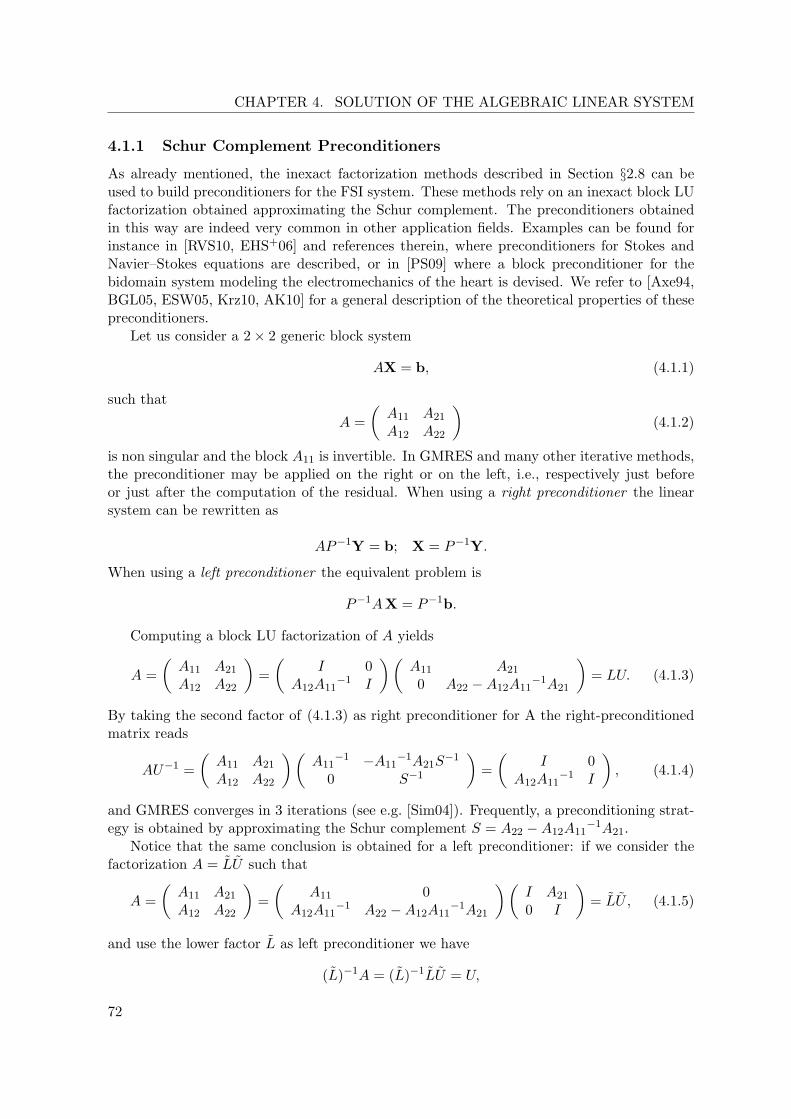
CHAPTER 4. SOLUTION OF THE ALGEBRAIC LINEAR SYSTEM
4.1.1 Schur Complement Preconditioners
As already mentioned, the inexact factorization methods described in Section §2.8 can beused to build preconditioners for the FSI system. These methods rely on an inexact block LUfactorization obtained approximating the Schur complement. The preconditioners obtainedin this way are indeed very common in other application fields. Examples can be found forinstance in [RVS10, EHS+06] and references therein, where preconditioners for Stokes andNavier–Stokes equations are described, or in [PS09] where a block preconditioner for thebidomain system modeling the electromechanics of the heart is devised. We refer to [Axe94,BGL05, ESW05, Krz10, AK10] for a general description of the theoretical properties of thesepreconditioners.
Let us consider a 2× 2 generic block system
AX = b, (4.1.1)
such that
A =(A11 A21
A12 A22
)(4.1.2)
is non singular and the block A11 is invertible. In GMRES and many other iterative methods,the preconditioner may be applied on the right or on the left, i.e., respectively just beforeor just after the computation of the residual. When using a right preconditioner the linearsystem can be rewritten as
AP−1Y = b; X = P−1Y.
When using a left preconditioner the equivalent problem is
P−1AX = P−1b.
Computing a block LU factorization of A yields
A =(A11 A21
A12 A22
)=(
I 0A12A11
−1 I
)(A11 A21
0 A22 −A12A11−1A21
)= LU. (4.1.3)
By taking the second factor of (4.1.3) as right preconditioner for A the right-preconditionedmatrix reads
AU−1 =(A11 A21
A12 A22
)(A11
−1 −A11−1A21S
−1
0 S−1
)=(
I 0A12A11
−1 I
), (4.1.4)
and GMRES converges in 3 iterations (see e.g. [Sim04]). Frequently, a preconditioning strat-egy is obtained by approximating the Schur complement S = A22 −A12A11
−1A21.Notice that the same conclusion is obtained for a left preconditioner: if we consider the
factorization A = LU such that
A =(A11 A21
A12 A22
)=(
A11 0A12A11
−1 A22 −A12A11−1A21
)(I A21
0 I
)= LU , (4.1.5)
and use the lower factor L as left preconditioner we have
(L)−1A = (L)−1LU = U,
72

4.1. BLOCK TRIANGULAR PRECONDITIONERS
which has similar spectral properties as (4.1.4). It is easy to compute the block inverse of L,as done for U , in terms of S−1 and A11
−1.Alternatively the reduced system
SX2 = b2 −A12A11−1b1, (4.1.6)
where X =[
X1
X2
]and b =
[b1
b2
], can be considered instead of (4.1.1). This system is
equivalent to the original one, and also in this case choosing a good preconditioner for (4.1.6)amounts to devising an approximation for the Schur complement matrix S.
An indicator for the quality of a preconditioner is the conditioning of the preconditionedsystem. If we solve the linear system (4.1.1) with Krylov iterations and left preconditionerP , then the conditioning can be represented by the condition number of P−1A
K(P−1A) =maxσ(P−1A)minσ(P−1A)
, (4.1.7)
where σ(A) denotes the set of singular values of a matrix A (see e.g. [QSS00]).The theoretical estimates for the condition number of block-preconditioned systems often
rely on the hypothesis that the system is positive (semi)definite. Let us consider the sets ofindexes V1, V2, and W = V1 × V2. In case matrix (4.1.2) is partitioned accordingly with V1
and V2, if the system is symmetric positive semidefinite and the block A11 is positive definite,then the condition number estimates for the system preconditioned using a Schur complementpreconditioner depends on the Cauchy–Bunyakowski–Schwarz (CBS) constant
γ = supw1∈W1,w2∈W2
wT1 Aw2
wT1 Aw1 wT
2 Aw212
, (4.1.8)
where
W1 =
v =[
v1
0
]∈W |v1 ∈ V1
W2 =
v =
[0v2
]∈W |v2 ∈ V2
.
In [Axe94, Ch.9.3] and [AK10] the condition number of the system (4.1.6) preconditionedwith P = A22 is shown to satisfy the following (sharp) bound: K(P−1S) ≤ 1
1−γ2 . For instancein the numerical FE approximation of a 2D diffusion problem, if the two blocks refer to twodifferent subdomain problems, the CBS constant is γ = 1−O(h), where h is the characteristicdimension of the triangulation. Thus the condition number behaves like O(h−1).
The same estimate holds if we build a preconditioner for the matrix in (4.1.3) by takingthe U factor and replacing the Schur complement S with A22, which leads to a block GSpreconditioner.
We refer to [Axe94, Ch.9], [AK10, KM09] for these and other examples of Schur comple-ments preconditioners and their condition number estimates depending on γ.
In the case of two subdomains, we consider the Steklov–Poincare approach, describedin Section §3.2 for the nonlinear case and which will also be discussed in Section §4.2. Thematrix A of a linear diffusion problem can be divided in three subproblems, one per subdomainproblem plus an interface problem. Reducing the problem to the interface by means of theSchur complements one can write the algebraic equivalent of (3.2.18) (notice that the algebraiccounterparts of the Steklov–Poincare operators are the Schur complements). Preconditioningthis system with one of the local Schur complements, as done for the nonlinear continuous
73

CHAPTER 4. SOLUTION OF THE ALGEBRAIC LINEAR SYSTEM
case in (3.2.20) using a Steklov–Poincare operator, leads to a system where the conditionnumber is constant, and in particular is independent of h. We say in these cases that thepreconditioner is optimal. A proof of this result can be found in [TW05].
4.1.2 Block Gauss–Seidel Preconditioners
Another classical strategy to build block triangular preconditioners leads to the block GSpreconditioners (which can be seen as a particular case of the block preconditioners discussedabove, where the Schur complement is approximated with a diagonal block). As for the Schurcomplements preconditioners, also the block GS preconditioners exploit the block structurenature of multiphysics problems.
Applied to matrix (4.1.2), a block GS preconditioner reads
PGS =(A11 0A12 A22
)=(
I 0A12A11
−1 I
)(A11 00 A22
), (4.1.9)
thus
P−1GS =
(A11
−1 0−A22
−1A12A11−1 A22
−1
)=(
I 0−A22
−1A12 I
)(A11
−1 00 A22
−1
).
The corresponding left-preconditioned system then reads
P−1GSA =
(A11
−1 00 A22
−1
)(A11 A21
0 S
). (4.1.10)
The robustness of these preconditioners have been tested for instance in [Hei04] for the FSIsystem.
4.2 Applications to the FSI system
In this section we report some popular solution methods discussed e.g. in [BQQ08a, DDFQ06,BNV08, GGNV10] with a different formalism (similar to the one used in Gee at al. [GKW10]).
We describe some common choices for the preconditioners in the FSI context. In particularwe focus on the block GS preconditioners, and we show how classical domain decompositionmethods (like most of the so called partitioned procedures in FSI) can be seen, when appliedto a linearized system, as block GS preconditioned Richardson methods.
We have already seen how to interpret classical domain decomposition methods as fixedpoint strategies (cf. Section §3.2). Without using a DD strategy at the continuous level,it is possible to work on the algebraic system and recover modularity using a block GSpreconditioner.
To clarify the ideas we present first a block GS preconditioner in the case of the GCEdiscrete algebraic system, and we extend the strategy to the Jacobian system of the nonlinearcase in a second step. We remark that the matrix in (2.7.12) has the same form as thefluid–structure blocks in (2.7.10), thus the preconditioning strategies devised for GCE canbe easily employed also in the other cases, by applying them to the fluid–structure part ofthe matrix. The specific way this is done is detailed in Section §4.2.4. Recalling the GCEalgebraic system (2.7.12) we can write a block GS iteration as follows
74

4.2. APPLICATIONS TO THE FSI SYSTEM
Cff CfΓ 0 0 0CΓf CΓΓ 0 0 0
0 0 Ns NsΓ 00 0 NΓs NΓΓ −I0 I 0 −I/δt 0
uf k+1
uf k+1Γ
dk+1s
dk+1sΓ
λk+1
=
rfn+1
rfΓn+1 − λkrsn+1
rsΓn+1
−(I/δt)dnsΓ
, (4.2.1)
where k represents the block GS iteration index and n+ 1 is the current time level.Writing equation (2.7.12) as AX = b and calling PND the matrix in (4.2.1) we can rewrite
the system (4.2.1) asPNDXk+1 = (PND −A)Xk + b,
which is the Richardson method preconditioned with PND (with acceleration parameter setto 1)
Xk+1 = Xk + PND−1(−AXk + b). (4.2.2)
The block GS preconditioner PND is also called Neumann–Dirichlet preconditioner, be-cause the Richardson method (4.2.2) corresponds to the Neumann–Dirichlet algorithm whenthe problem is linear (see [QV99]).
To simplify the notations in the following part of this section we condense the fluid andthe solid blocks
C =(Cff CfΓ
CΓf CΓΓ
)N =
(Ns NsΓ
NΓs NΓΓ
).
Furthermore we call O and I the null and identity matrices respectively, regardless of thenumbers of block rows/columns, so that the GCE matrix in system (2.7.12) reads with thenew notations
A =
C O 0
I
O N 0−I
0 I 0 −I/δt 0
. (4.2.3)
It is possible to write the Dirichlet–Neumann method as a preconditioned Richardsonmethod as well. In our implementation we test the following two forms of Dirichlet–Neumannpreconditioners:
P(1)DN =
C O 0
I
O N 00
0 I 0 −I/δt 0
(4.2.4)
and
P(2)DN =
C O 0
I
O N 0−I
0 I 0 0 0
. (4.2.5)
In both cases the Neumann solid problem is decoupled from the other equations, while thelast block row represents the Dirichlet coupling condition for the fluid problem.
75
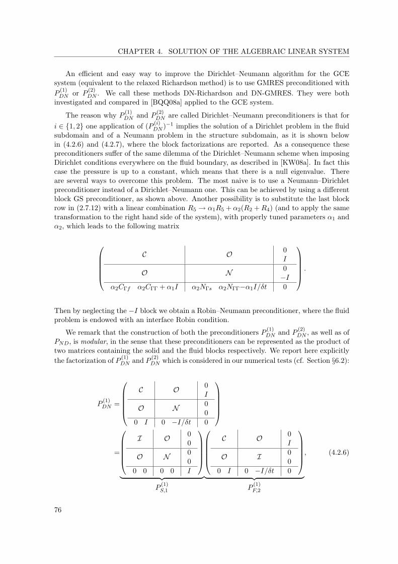
CHAPTER 4. SOLUTION OF THE ALGEBRAIC LINEAR SYSTEM
An efficient and easy way to improve the Dirichlet–Neumann algorithm for the GCEsystem (equivalent to the relaxed Richardson method) is to use GMRES preconditioned withP
(1)DN or P (2)
DN . We call these methods DN-Richardson and DN-GMRES. They were bothinvestigated and compared in [BQQ08a] applied to the GCE system.
The reason why P (1)DN and P
(2)DN are called Dirichlet–Neumann preconditioners is that for
i ∈ 1, 2 one application of (P (i)DN )−1 implies the solution of a Dirichlet problem in the fluid
subdomain and of a Neumann problem in the structure subdomain, as it is shown belowin (4.2.6) and (4.2.7), where the block factorizations are reported. As a consequence thesepreconditioners suffer of the same dilemma of the Dirichlet–Neumann scheme when imposingDirichlet conditions everywhere on the fluid boundary, as described in [KW08a]. In fact thiscase the pressure is up to a constant, which means that there is a null eigenvalue. Thereare several ways to overcome this problem. The most naive is to use a Neumann–Dirichletpreconditioner instead of a Dirichlet–Neumann one. This can be achieved by using a differentblock GS preconditioner, as shown above. Another possibility is to substitute the last blockrow in (2.7.12) with a linear combination R5 → α1R5 + α2(R2 +R4) (and to apply the sametransformation to the right hand side of the system), with properly tuned parameters α1 andα2, which leads to the following matrix
C O 0
I
O N 0−I
α2CΓf α2CΓΓ + α1I α2NΓs α2NΓΓ−α1I/δt 0
.
Then by neglecting the −I block we obtain a Robin–Neumann preconditioner, where the fluidproblem is endowed with an interface Robin condition.
We remark that the construction of both the preconditioners P (1)DN and P (2)
DN , as well as ofPND, is modular, in the sense that these preconditioners can be represented as the product oftwo matrices containing the solid and the fluid blocks respectively. We report here explicitlythe factorization of P (1)
DN and P (2)DN which is considered in our numerical tests (cf. Section §6.2):
P(1)DN =
C O 0
I
O N 00
0 I 0 −I/δt 0
=
I O 0
0
O N 00
0 0 0 0 I
︸ ︷︷ ︸
P(1)S,1
C O 0
I
O I 00
0 I 0 −I/δt 0
︸ ︷︷ ︸
P(1)F,2
, (4.2.6)
76

4.2. APPLICATIONS TO THE FSI SYSTEM
while for P (2)DN :
P(2)DN =
C O 0
I
O N 0−I
0 I 0 0 0
=
C O 0
I
O I 00
0 I 0 0 0
︸ ︷︷ ︸
P(2)F,1
I O 0
0
O N 0−I
0 0 0 0 I
︸ ︷︷ ︸
P(2)S,2
. (4.2.7)
We have shown that the application of the inverse preconditioner P−1 amounts to invertingthe fluid and structure factors separately. In practice for a vector X the computation ofe.g. P (2)
F,1X and P(2)S,2X is performed by means of an LU factorization of the matrices P (2)
F,1
and P(2)S,2 , or by GMRES (or CG) iterations. The former strategy is appealing because the
factorizations computed can be reused throughout the solution of the global linear system,however memory issues may limit the size of the problem considered. The latter consists inusing e.g. preconditioned GMRES iterations for the fluid problem and preconditioned CG forthe structure one. However this strategy introduces inner iterations to solve the subproblems.Since the number of inner iterations usually increases when the number of processors grows,even though the outer iterations remain constant, the total number of iterations (which isthe product of the two) grows too fast. A possible remedy could be the use of a flexibleGMRES with a fixed number of inner iterations. This has been done in [EHS+08, EHST03]for the Navier–Stokes equations. Our solution is explained in the next section and consists insubstituting the factors with preconditioners computed with classical strategies (e.g. domaindecomposition) tailored on the problem.
We describe in the three following subsections some other block preconditioners for theGCE system (2.6.2). Most of these preconditioning techniques are implemented in the FElibrary LifeV. We anticipate that the strategies devised for the GCE approach can be employedas well in the other cases for the first two blocks (corresponding to the fluid and structureequations), as shown in Section §4.2.4.
4.2.1 Robin–Robin Preconditioners
A generalization of the Dirichlet–Neumann approach is the Robin-Robin one [BNV08], asdiscussed in Section §3.2. Substituting, in the GCE time-discretized equation (2.6.2) in strongform, the Neumann and Dirichlet coupling conditions with Robin transmission conditions
77

CHAPTER 4. SOLUTION OF THE ALGEBRAIC LINEAR SYSTEM
leads to the following
ρfδtun+1 + ρf (un −wn+1) · ∇xun+1 −∇x·σfn+1 = ffn+1 in Ωft n+1
∇x·un+1 = 0 in Ωft n+1
αf (un+1 Atn+1 − δtdn+1s ) + σn+1
f · nf + Πn+1 · ns = 0 on Γ (4.2.8)
ρsδttdn+1s −∇bx·Πn+1 = fsn+1 in Ωs
αs(un+1 Atn+1 − δtdn+1s ) + σn+1
f · nf + Πn+1 · ns = 0 on Γ
+conditions on the external boundaries.
The algebraic system deriving from (4.2.8) readsCff CfΓ 0 0CΓf CΓΓ + αfI NΓs NΓΓ − αfI/δt
0 0 Ns NsΓ
CΓf CΓΓ + αsI NΓs NΓΓ − αsI/δt
ufn+1
uΓn+1
dn+1s
dn+1sΓ
=
rf
rsΓn+1 + rfΓn+1 − αf dnsΓ/δtrs
rsΓn+1 + rfΓn+1 − αsdnsΓ/δt
. (4.2.9)
Here we chose not to introduce the multiplier λ for the sake of clarity, however the systemcan be easily rewritten in the augmented form (2.7.12).
As done in the previous case, we can write a block GS iteration for this system discretizedin space and time.
Cff CfΓ 0 0CΓf CΓΓ + αfI 0 0
0 0 Ns NsΓ
CΓf CΓΓ + αsI NΓs NΓΓ − αsI/δt
uf k+1
uΓk+1
dk+1s
dk+1sΓ
=
rfn+1
NΓsdks + (αfI/δt−NΓΓ)dksΓ + rsΓn+1 + rfΓn+1 − αf dnsΓ/δt
rsrsΓn+1 + rfΓ
n+1 − αsdnsΓ/δt
. (4.2.10)
With a method analogous to that used in the Dirichlet–Neumann case it is possible toshow that the Robin–Robin method can be rewritten as system (2.7.12) preconditioned with
PRR =
I 0 0 00 1
αf−αs I 0 1αs−αf I
0 0 I 00 αs
αs−αf I 0 αfαf−αs I
Cff CfΓ 0 0CΓf CΓΓ + αfI 0 0
0 0 Ns NsΓ
CΓf CΓΓ + αsI NΓs NΓΓ − αsI/δt
. (4.2.11)
In fact defining
Q =
I 0 0 00 αfI 0 I0 0 I 00 αsI 0 I
,
78

4.2. APPLICATIONS TO THE FSI SYSTEM
and
P =
Cff CfΓ 0 0CΓf CΓΓ + αfI 0 0
0 0 Ns NsΓ
CΓf CΓΓ + αsI NΓs NΓΓ − αsI/δt
,
if AX = b represents equation (2.7.12), we can write the system (4.2.9) as
PXk+1 = (P −QA)Xk +Qb,
and thusQ−1PXk+1 = Q−1PXk −AXk + b,
which is the Richardson method preconditioned with PRR = Q−1P .
4.2.2 Dirichlet–Dirichlet Preconditioners
The preconditioning strategy that we are going to describe is reported here formally, but itis not tested in the numerical applications part since it is not implemented yet in LifeV.
Let us recall the definition of the Steklov–Poincare operators for the fluid and structuresubdomains (3.2.19). Each application of one of these operators implies the solution of asubproblem with Dirichlet coupling conditions on the interface. The equation
Σf (dsΓ) + Σs(dsΓ) = 0 on Γ (4.2.12)
represents the Steklov–Poincare formulation of the FSI problem, and expresses the weak stresscontinuity across the interface. The solution of equation (4.2.12), as shown in Section §3.2, canbe viewed as the result of a further partition of the original problem, where we solve separatelyan equation for the fluid and solid internal domains and an equation for the interface domainwhich is coupled with both. We consider again the GCE time discretization, and we recall thatthe discrete Steklov–Poincare operators are the Schur complements on the interface degreesof freedom of the matrix in (2.7.12).
As done in Section §3.2 we introduce the multiplier ηn+1 = dn+1sΓ representing the interface
displacement. The system in strong form discretized in time reads
ρfδtun+1 + ρf (un −wn+1) · ∇xun+1 −∇x·σfn+1 = ffn+1 in Ωft n+1
∇bx·un+1 = 0 in Ωft n+1
un+1 − δtηn+1 = 0 on Γ
ρsδttdn+1s −∇bx·(Π)n+1 = fsn+1 in Ωs
dn+1sΓ = ηn+1 on Γ0 (4.2.13)
Πn+1 · ns + (σf )n+1 · nf = 0 on Γ+conditions on the external boundaries.
The resulting linear system is naturally written in augmented form asCff CfΓ 0 0 0
0 I 0 0 −I/δt0 0 Ns NsΓ 00 0 0 I −ICΓf CΓΓ NΓs NΓΓ 0
ufn+1
uΓn+1
dn+1s
dn+1sΓ
ηn+1
=
rfn+1
−ηn/δtrsn+1
0rsΓn+1 + rfΓ
n+1
. (4.2.14)
79

CHAPTER 4. SOLUTION OF THE ALGEBRAIC LINEAR SYSTEM
Notice that all the entries in the fourth and the last columns can be interchanged, because ofthe condition ηn+1 = dn+1
sΓ . The algebraic counterpart of the Steklov–Poincare formulationrecalled here could be obtained by computing the Schur complements of the fluid and structureblocks, in order to eliminate the variables ufn+1,uΓ
n+1, dn+1s , dn+1
sΓ in (4.2.14), obtaining alinear system in ηn+1. However in this section, as done for the Dirichlet–Neumann case,we describe a preconditioner for the whole FSI problem (without restricting to a subset ofvariables) whose computation involves the same type of problems encountered when solvinga Richardson iteration for the Schur complements system (i.e., two Dirichlet problems for thefluid and structure).
System (4.2.14) can be solved with block GS iterations, or a block GS preconditioner canbe used for GMRES iterations on the system (4.2.14).
We call Dirichlet–Dirichlet preconditioner the following:
PDD =
Cff CfΓ 0 0 0
0 I 0 0 00 0 Ns NsΓ 00 0 0 −I 0CΓf CΓΓ NΓs 0 NΓΓ
.
Instead of considering Dirichlet problems FD and SD in the fluid and solid blocks we cantake Neumann ones (FN and SN , see remark 3.2.6). Then stressing the velocity continuitycoupling condition is obtained by imposing the equality between the inverse of the Steklov–Poincare operators (which are Neumann to Dirichlet maps). We obtain (with the same stepsretrieved for the previous case) the following linear system
C O 0I
O N 0−I
0 I 0 −I/δt 0
ufn+1
uΓn+1
dn+1s
dn+1sΓ
λn+1
=
rfn+1
rfΓn+1
rsn+1
rsΓn+1
−dnsΓ/δt
. (4.2.15)
This time the multiplier is denoted with λn+1 and it represents the residual of the two equa-tions on the interface.
Sometimes in practical implementations the usage of preconditioners like PDN in (4.2.4)or (4.2.5) causes problems because of the zero diagonal block in the lower-right corner. Toavoid this problem we can perform a change of variables in (4.2.1) derived from the fourthrow of the system (2.7.12):
dn+1sΓ = N−1
ΓΓ (−NΓsdn+1s + λn+1 + rsΓn+1).
This change of variable in the last equation of (4.2.15) leads to the following system
C 0
0I
O N 0−I
0 NΓΓ NΓs/δt 0 −I/δt
ufn+1
uΓn+1
dn+1s
dn+1sΓ
λn+1
=
rfn+1
rfΓn+1
rsn+1
rsΓn+1
−NΓΓdnsΓ/δt− rsΓn+1/δt
.
(4.2.16)
80

4.2. APPLICATIONS TO THE FSI SYSTEM
A block GS iteration readsC O 0
0
O N 00
0 NΓΓ NΓs/δt 0 −I/δt
uf k+1
uΓk+1
dk+1s
dk+1sΓ
λk+1
=
rfn+1
rfΓn+1 − λkrsn+1
rsΓn+1 + λk
−NΓΓdnsΓ/δt− rsΓn+1/δt
.
(4.2.17)The corresponding block GS preconditioner involves two Neumann subproblems, thus we callit PNN .
Remark 4.2.1. In the classical domain decomposition nomenclature this preconditioner cor-responds indeed to a Neumann–Neumann preconditioner, while PDD corresponds to a FETI(Finite Elements Tearing and Interconnecting) preconditioner [TW05].
4.2.3 Other Additive Preconditioners
Another possibility concerning the preconditioning strategies for the system (2.7.12) is torewrite the matrix in (4.2.15) as sum of two matrices A = A(1) +A(2) and then approximateits inverse withA−1 ≈ A−1
(1)+A−1(2). We call these types of preconditioners additive (see [AK10]).
To further simplify the notations here we introduce the following convention I =(
0I
)and
IT =(
0 I).
We have
A =
C 0 I0 N −IIT −IT /δt 0
=
=
12C 0 I0 1
2N −12I
12IT 0 0
+
12C 0 00 1
2N −12I
12IT −IT /δt 0
= A(1) +A(2).
A block factorization for these two matrices can easily be computed, in fact
A(1) =
12C 0 I0 I 0
12IT 0 I
I 0 00 1
2N −12I
0 0 I
,
while
A(2) =
12C 0 00 I 0
12IT 0 I
I 0 00 1
2N −12I
0 −IT /δt -I
.
Notice that in the factorization of the matrix A(1) we added an identity block (the boxedblocks highlighted above) to avoid that some factors have null diagonal blocks. The matrixA(1) involves two decoupled problems. Without the identity block added on the lower-rightcorner these problems would have been of Dirichlet type on the fluid and of Neumann type onthe solid. However the introduction of the identity block mixes the two coupling conditions inthe first factor generating a Robin fluid problem. The same consideration holds for the blockfactorization of the matrix A(2): without the highlighted identity block its inversion would
81

CHAPTER 4. SOLUTION OF THE ALGEBRAIC LINEAR SYSTEM
imply the solution of a Neumann problem for the fluid and a Dirichlet one for the solid, whilewhen the identity block is added the solid problem becomes of Robin type.
Another possible splitting of the matrix A would be
A = A(1) + A(2) =
12C 0 I0 1
2N −I0 0 I
+
12C 0 00 1
2N 0I −I/δt −I
.
with the following factorizations:
A(1) =
12C 0 I0 I 00 0 I
I 0 00 1
2N −I0 0 I
,
and
A(2) =
12C 0 00 I 0I 0 I
I 0 00 1
2N 00 −I/δt −I
.
The inversion of these two blocks implies again two Neumann and two Dirichlet solutions ofthe subdomain problems.
Remark 4.2.2. We notice that for a splitting like A = A(1) + A(2), the situation in whichA(1) = A(2) = 1
2A would lead to the exact factorization of A, thus a situation in which A(1) iscloser to A(2) is preferable.
4.2.4 Extension to Other Time Discretizations
The considerations made for the GCE time discretization hold true also for the other variants,in particular we show here a block GS preconditioner for the Jacobian matrix of the fullyimplicit system JFI .
The Jacobian matrix in (3.1.2) reads
JFI =
DufCf DuΓCf 0 0 0 DbdfCf DbdfΓCf
DufCΓ DuΓCΓ 0 0 I DbdfCΓ DbdfΓCΓ
0 0 DbdsNs DbdsΓNs 0 0 00 0 DbdsNΓ DbdsΓNΓ -I 0 00 I 0 −I/δt 0 0 00 0 0 0 0 Hff HfΓ
0 0 0 −I 0 0 I
, (4.2.18)
where the block rows correspond, from top to bottom, to the linearized fluid problem, thesolid problem, the condition on the velocity continuity at the interface, and the geometryproblem. We used the abridged notationsDxCf = DxCff+DxCfΓ, DxCΓ = DxCΓf+DxCΓΓ,DxNs = DxNss +DxNsbΓ, and DxNbΓ = DxNbΓs +DxNbΓbΓ, for any variable x. For x = df andx = dfΓ, Dx represents the shape derivatives introduced in Section §3.4.
82
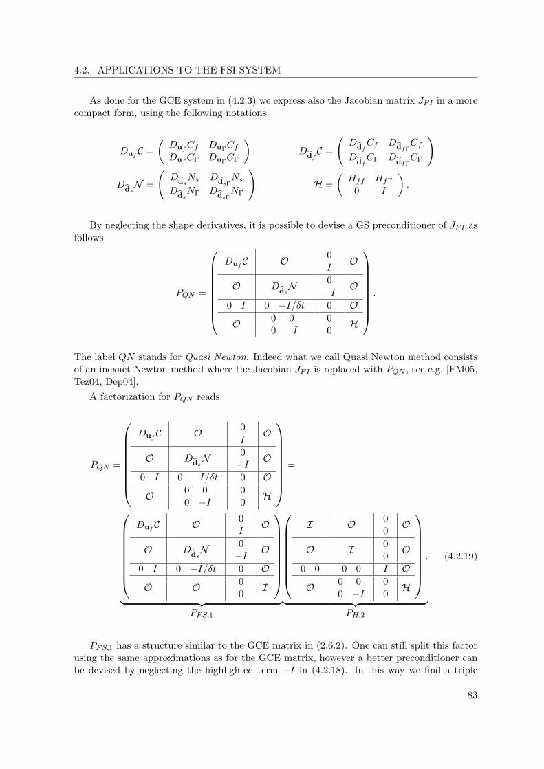
4.2. APPLICATIONS TO THE FSI SYSTEM
As done for the GCE system in (4.2.3) we express also the Jacobian matrix JFI in a morecompact form, using the following notations
DufC =(DufCf DuΓCfDufCΓ DuΓCΓ
)DbdfC =
(DbdfCf DbdfΓ
Cf
DbdfCΓ DbdfΓCΓ
)
DbdsN =
(DbdsNs DbdsΓNs
DbdsNΓ DbdsΓNΓ
)H =
(Hff HfΓ
0 I
).
By neglecting the shape derivatives, it is possible to devise a GS preconditioner of JFI asfollows
PQN =
DufC O 0I
O
O DbdsN 0−I O
0 I 0 −I/δt 0 O
O 0 00 −I
00
H
.
The label QN stands for Quasi Newton. Indeed what we call Quasi Newton method consistsof an inexact Newton method where the Jacobian JFI is replaced with PQN , see e.g. [FM05,Tez04, Dep04].
A factorization for PQN reads
PQN =
DufC O 0I
O
O DbdsN 0−I O
0 I 0 −I/δt 0 O
O 0 00 −I
00
H
=
DufC O 0I
O
O DbdsN 0−I O
0 I 0 −I/δt 0 O
O O 00
I
︸ ︷︷ ︸
PFS,1
I O 00O
O I 00O
0 0 0 0 I O
O 0 00 −I
00H
.
︸ ︷︷ ︸PH,2
(4.2.19)
PFS,1 has a structure similar to the GCE matrix in (2.6.2). One can still split this factorusing the same approximations as for the GCE matrix, however a better preconditioner canbe devised by neglecting the highlighted term −I in (4.2.18). In this way we find a triple
83
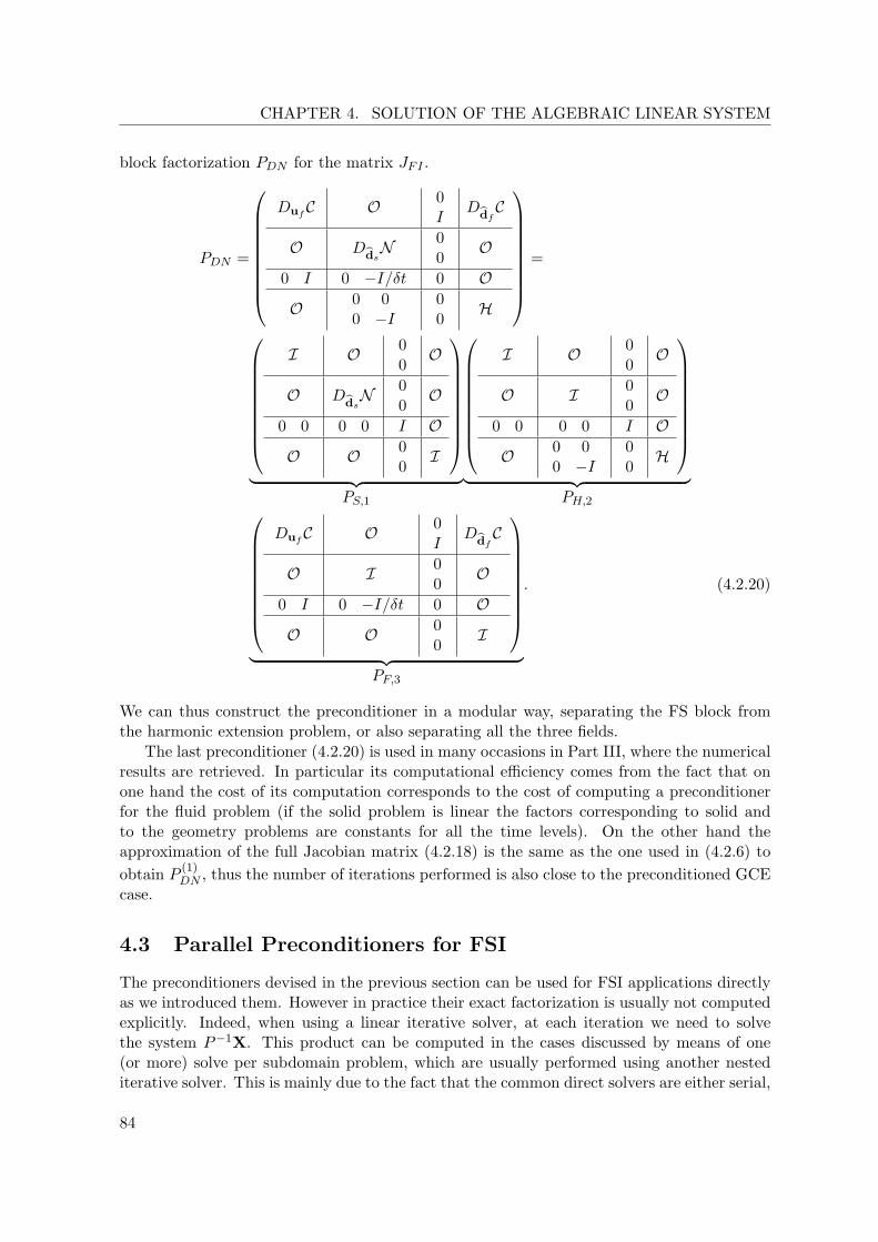
CHAPTER 4. SOLUTION OF THE ALGEBRAIC LINEAR SYSTEM
block factorization PDN for the matrix JFI .
PDN =
DufC O 0I
DbdfCO DbdsN 0
0O
0 I 0 −I/δt 0 O
O 0 00 −I
00
H
=
I O 00O
O DbdsN 00O
0 0 0 0 I O
O O 00I
︸ ︷︷ ︸
PS,1
I O 00O
O I 00O
0 0 0 0 I O
O 0 00 −I
00H
︸ ︷︷ ︸
PH,2
DufC O 0I
DbdfCO I 0
0O
0 I 0 −I/δt 0 O
O O 00
I
︸ ︷︷ ︸
PF,3
. (4.2.20)
We can thus construct the preconditioner in a modular way, separating the FS block fromthe harmonic extension problem, or also separating all the three fields.
The last preconditioner (4.2.20) is used in many occasions in Part III, where the numericalresults are retrieved. In particular its computational efficiency comes from the fact that onone hand the cost of its computation corresponds to the cost of computing a preconditionerfor the fluid problem (if the solid problem is linear the factors corresponding to solid andto the geometry problems are constants for all the time levels). On the other hand theapproximation of the full Jacobian matrix (4.2.18) is the same as the one used in (4.2.6) toobtain P (1)
DN , thus the number of iterations performed is also close to the preconditioned GCEcase.
4.3 Parallel Preconditioners for FSI
The preconditioners devised in the previous section can be used for FSI applications directlyas we introduced them. However in practice their exact factorization is usually not computedexplicitly. Indeed, when using a linear iterative solver, at each iteration we need to solvethe system P−1X. This product can be computed in the cases discussed by means of one(or more) solve per subdomain problem, which are usually performed using another nestediterative solver. This is mainly due to the fact that the common direct solvers are either serial,
84
4.3. PARALLEL PRECONDITIONERS FOR FSI
and thus require too much memory and time resources on large problems, or are not scalablein parallel, which produces a bottleneck in the simulation. To avoid these nested iterativesolutions one possibility is to approximate the subdomain blocks with other blocks whosefactorization requires neither subiterations nor parallel direct solutions. These approximationsare scalable preconditioners for the subproblems, which need to be computed in parallel andwhich should not increase much the conditioning of the global preconditioned system. Thefactorizations described above are used in this section to build the parallel preconditionersimplemented in our code (some of them are reported also in [CDFQ11]).
4.3.1 State of the Art
The research in the field of parallel preconditioning strategies is both challenging and neces-sary for most of the applications in numerical analysis. Theoretical important results havebeen achieved during the past decades, providing bounds for the condition number of thepreconditioned systems. However the problem is still open, e.g. for indefinite problems thetheory is not so developed as for symmetric positive definite (s.p.d.) problems. In this sec-tion all the estimates reported indeed refer to the case of a s.p.d. matrix coming from thediscretization of a linear second order elliptic problem in 3D.
On the applications side there have been many recent advances as well. The availabil-ity of massively parallel architectures have pushed the software towards the developmentof highly scalable libraries for linear algebra computations. Domain decomposition andmultigrid techniques have become standard approaches to handle parallelism, heuristic al-gorithms and coloring techniques have been devised for the domain partition in order toachieve an effective load balance between the processors and to minimize the communica-tion [CP08, SKK02, CBD+07]. Domain decomposition and multigrid preconditioners havebeen tested on a large variety of applications and they have shown to be effective for manyFE computations (see e.g. [BCA+10, LSS+09, Sal06, KR10, TF01, PW11] and referencestherein). Many software packages allow to build these preconditioners from the system ma-trix, without using geometrical informations. The preconditioners built in this way are calledalgebraic (while the classical ones are geometrical), and are the most used in practical appli-cations, especially when the geometry does not allow a structured partition in subdomains.Most of these preconditioners rely on a solution of one or more coarse problems, which canalso be built using only informations at the algebraic level e.g. through smoothed aggregationtechniques, see e.g. [TW05, Ch.3.10] [VMB96].
In this subsection we report theoretical estimates for the condition number of some of themost popular preconditioners used in parallel solvers for FSI. We focus in particular on domaindecomposition preconditioners referring to [TW05, QV99] for a more detailed description.
Domain decomposition methods can be roughly divided into overlapping and iterativesubstructuring. The formers (e.g. Schwarz methods) imply a partition in overlapping subdo-mains which covers the original domain, while the latter (e.g. Dirichlet–Neumann, Neumann–Neumann, FETI, BDDC) involve the partition in non-overlapping subdomains, and the re-striction of the subproblems defined on each subdomain to their boundary through Schurcomplements. A domain decomposition method is called one level when no coarse grid com-ponent is present, i.e., there is no information exchange between non neighboring subdomains.It is unavoidable that the condition number of a one level preconditioner P1l is subject toa bound like K(P1l
−1A) ≤ O(
1δ2H2
)(one–level additive Schwarz preconditioners applied to
a Poisson problem), where A is the finite elements system matrix, δ is the thickness of the
85

CHAPTER 4. SOLUTION OF THE ALGEBRAIC LINEAR SYSTEM
overlap and H is the maximum diameter of the subdomains. The coefficient 1H2 is due to the
fact that there is no exchange of information between two subdomains which are not adja-cent, and it is related to the fact that we consider a second order elliptic differential operator.This is similar to the condition number of the stiffness matrix in finite elements, where thedependence on 1
h2 can be seen as a consequence of a scaling argument [TW05].To avoid this dependence on 1
H2 it is sufficient to add a coarse problem component to thepreconditioner, subject to a set of assumptions. This and similar ideas were devised at theend of the eighties, among others by Bramble, Pasciak, Dryja, Wildlund. The bound for thecondition number becomes
K(P2l−1A) ≤ O
(1 +
(log
H
h
)2),
where P2l is an iterative substructuring preconditioner without overlap like FETI, Neumann–Neumann, BDDC. For the two-levels additive overlapping Schwarz preconditioners the esti-mate becomes
K(P2l−1A) ≤ O
(1 +
H
δ
).
Since the coarse problem is usually solved by a direct method, and since due to its limitedsize its solution is generally fast, in many parallel implementations every processor solves thecoarse problem independently, which avoids the inter-processors communication. Howeversometimes in massively parallel computations also the coarse problem is too large to be solvedserially on every processor. In these cases the partitioning can be performed recursively onthe coarse problems, generating a multilevel preconditioner in which only the coarsest levelis solved directly on each core.
A very popular choice consists in the algebraic domain decomposition preconditioners.In this case the coarse problem is computed through an algebraic interpolation-restrictionoperator which has to be defined for each level. A well known algorithm to generate the coarsespace is the smoothed aggregation technique developed by Vanek, Brenzina and coauthors atthe end of the nineties [VMB96]. For these methods, applied to the multilevel overlappingSchwarz preconditioner, the same bound for the condition number holds as in the case ofgeometrical coarse problem [Sar02].
An “alternative” preconditioning strategy which is very common and effective consists inusing multigrid preconditioners. As for the Schwarz strategy, the multigrid method can usu-ally be interpreted as a preconditioned Richardson method, and the multigrid preconditionercan be used in other iterative schemes such as GMRES. It consists of a multilevel strategy, inwhich each level is solved inexactly, and a prescribed number of iterations of a chosen iterativemethod (smoother) is performed at each level. In the coarsest level the problem is usuallysolved exactly with a direct method. The multigrid strategy is usually tuned for the specificapplication, featuring V or W cycles, pre or post smoothing, different smoothers and aggre-gation techniques. We refrain from discussing all the possibilities, and we refer to [KM09] fora survey on this subject and for an overview of a similar preconditioning technique (AlgebraicMultilevel Iteration, AMLI, first introduced by Axelsson and Vassilevski [AV89]), which canbe seen as a generalization of the algebraic multigrid (AMG) preconditioner.
The algebraic multigrid method has been popularized by Ruge and Stuben in 1987 [RS87],while an algebraic multigrid preconditioner was used recently in e.g. [PS09, LSS+09], see also[Not10] and references therein for a spectral analysis.
86

4.3. PARALLEL PRECONDITIONERS FOR FSI
In [BC10b] a 2D FSI solution obtained using an additive Schwarz preconditioner with andwithout the coarse problem is compared. There the presence of a coarse problem seems togreatly improve the condition number of the FSI system. In that case the weak scalabilityis tested: the size of the problem is increased with the number of processors by refining themesh.
A multigrid preconditioner for FSI problems is described in [GKW10]. There the conver-gence rate is tested with respect to the space discretization, showing independence of h forthe preconditioner considered.
Remark 4.3.1. Although domain decomposition and multigrid preconditioners have a dif-ferent origin, the difference between them is small. Indeed if a software implementation isgeneral enough it can embed both the strategies within the same code (see e.g. the ML packagein Trilinos6).
The preconditioners that we use in the next chapter are based on the algebraic additiveSchwarz preconditioner (AAS) that we briefly overview here, referring to the aforementionedliterature for the details. We consider the generic linear system AX = b (e.g. the discretizationof system (3.1.2)). We call V ⊆ Rn the discrete space in which the solution of the linear systemis defined. Following the notations used in [CK02], we introduce the set of indexes S =1 . . . n representing the degrees of freedom of the system. Given an overlapping partitionof S in I subsets, Si1≤i≤I , we define the subspaces Vi ⊆ V as Vi = X = (v1, . . . vn)T ∈Rn|vk = 0 if k /∈ Si of dimension ni. Next we introduce the restriction matrix Ri ∈ Rni×n
such that (Ri)ljδjk = δlk, l ∈ Si, k, j ∈ S and δ is the Kronecker symbol. The prolongationmatrix RTi ∈ Rn×ni transforms a short vector of ni components into one with n componentsby keeping the original components and setting to zero the new ones. In this framework wedefine the one level AAS preconditioner associated to A as
PAS(A)−1 =I∑i=1
RTi (RiARTi )−1Ri. (4.3.1)
As mentioned above it is possible to add a coarse component (corresponding to i = 0) toimprove the condition number when the number of subdomains increases. The parallel struc-ture of our code7 includes a mesh partitioner based on the library ParMETIS, AAS and AMGpreconditioners handled by the IFPACK and ML packages embedded in the Trilinos library.
4.3.2 Composed Preconditioners for Geometry–Convective Explicit FSI
In this section we develop the block–representation of the preconditioners for the matrix Ain (2.7.12). This section links the study of the block preconditioner carried out in Section §4.2to the classical domain decomposition preconditioners described above. The composition ofthe two strategies leads to the parallel preconditioners that we developed and that are testedand applied in the third part of this work.
The approach that we advocate consists in substituting the fluid and solid factors withsuitable preconditioners, whose factorization can be computed in parallel. For example, withthe notations (4.2.6), instead of P (1)
DN = P(1)S,1P
(1)F,2 or P (2)
DN = P(2)F,1P
(2)S,2 , we use, respectively,
6http://trilinos.sandia.gov7LifeV, http://www.lifev.org
87
CHAPTER 4. SOLUTION OF THE ALGEBRAIC LINEAR SYSTEM
PAS−DN1 = PAS(P (1)S,1)PAS(P (1)
F,2) or PAS−DN2 = PAS(P (2)F,1)PAS(P (2)
S,2). According to the do-main decomposition terminology this choice corresponds to employ inexact solvers for thesolid and fluid subdomains. A spectral analysis for a similar kind of block triangular pre-conditioners for stabilized saddle point problems, with symmetric positive definite diagonalblocks, is carried out e.g. in [Kla98, Sim04], while in [GKW10] a similar strategy is used inFSI context, where the blocks corresponding to all three fields are substituted with AMGpreconditioners. With this approach we avoid the inner iterations, since we can solve thelocal inexact problems by LU factorization.
A numerical comparison of the following preconditioning techniques is presented in Sec-tion §6.2 for the GCE time discretized system:
1. one–level AAS preconditioner built using the matrix A in (2.7.12): PAS(A) ;
2. one–level AAS preconditioner built using an approximation of the type (4.2.4), obtainedby neglecting the block −I in matrix (2.7.12): PAS−DN1;
3. one–level AAS preconditioner built using a different block GS approximation (4.2.5),obtained neglecting the term −I/δt in (2.7.12): PAS−DN2.
The preconditioners PAS−DN1 and PAS−DN2, besides preserving the modularity in theirconstruction, have similar or better behavior than PAS(A) when increasing the number ofprocessors. Furthermore, their factorization is cheaper in terms of computational time andmemory usage than building the factorization of the whole matrix A. In our framework, onecan choose different preconditioning techniques for the different sub-blocks, which is appealingfor multiphysics systems, since physics-specific preconditioners can be used.
4.3.3 Composed Preconditioners for Geometry Implicit FSI
For what concerns the fully implicit system, we consider in the following four different pre-conditioners:
• PAS(JFI);
• PAS−QN = PAS(PQN );
• PAS−GS = PAS(PFS,1)PAS(PH,2) where the factorization is the one reported in (4.2.19);
• PAS−DN = PAS(PS,1)PAS(PH,2)PAS(PF,3), with the factorization reported in (4.2.20).
By using a linear form for the convective term, i.e., choosing the convective explicit timediscretization, we can isolate the geometrical nonlinearity and investigate its effect on theprecision and stability of the system. Furthermore in our applications we have observedthat the behavior of the same preconditioner in the CE and FI cases is not very different.As discussed extensively in the previous chapter the geometrical nonlinearity can be solvede.g. with fixed–point iterations, inexact or exact Newton. The latter approach involves thecomputation of the shape derivatives which are reported in Section §3.4.1. We remark thatin case of linear elasticity for the solid problem building PAS−DN is as cheap as one fluidpreconditioner computation, since the factors related to the harmonic extension problem andto the solid problem are constant throughout the whole simulation and thus can be reused atevery time step.
88

4.3. PARALLEL PRECONDITIONERS FOR FSI
4.3.4 Spectral Analysis
Let us address the general framework of a 4-blocks matrix
A =(A11 A21
A12 A22
), (4.3.2)
where the block lines correspond to different coupled problems, the coupling being expressedby the matrices A12 and A21. The only a-priori assumption on the matrices A, A11 and A22
is that they are invertible, therefore the following analysis holds true for any linear systemwhose matrix has a 4-blocks structure like (4.3.2) with nonsingular diagonal blocks.
The idea is to replace the diagonal blocks A11 and A22 of the preconditioner PGS (4.1.9)by suitable preconditioners P1 and P2. In the following we estimate the influence of thisapproximation on the conditioning of the system. To this end we suppose that we havean estimate for the condition number of the two preconditioned blocks. Calling σmax
A =maxσ(σ(A)) and σmin
A = minσ(σ(A)) respectively the maximum and the minimum singularvalues for the matrix A, then for i ∈ 1, 2
δi = K(P−1i Ai) = σmax
P−1i Ai
/σminP−1i Ai
. (4.3.3)
We introduce a preconditioner of the form
P =(
P1 0A12 αP2
), (4.3.4)
where α is an arbitrary positive scalar. In order to bound the condition number of the matrixP−1A we compute explicitly P−1 as follows
P−1 =(
P−11 0
− 1αP−12 A12P
−11
1αP−12
).
Then the preconditioned system can be factored as
P−1A =(I 0Σ I
)(P−1
1 00 1
αP−12
)(A11 A21
0 S
), (4.3.5)
where Σ = 1αP−12 A12(A−1
1 P1 − I).An upper bound of the condition number for the preconditioned system can be obtained
using the inequality K(AB) ≤ K(A)K(B). We first find the singular values of the blocklower triangular factor (that we note L).
Proposition 4.3.1. The maximum and minimum singular values of L satisfy
σmaxL =
√1 +
(σmaxΣ )2 +
√(σmax
Σ )4 + 4(σmaxΣ )2
2, (4.3.6)
and
σminL =
√1 +
(σmaxΣ )2 −
√(σmax
Σ )4 + 4(σmaxΣ )2
2. (4.3.7)
89

CHAPTER 4. SOLUTION OF THE ALGEBRAIC LINEAR SYSTEM
Proof. By the definition of the singular values we have
(σmaxL )2 = max(eigs(LTL)),
where
LTL = I +(
ΣTΣ ΣT
Σ 0
).
Let us consider the matrix on the right: its null eigenvalues correspond to unitary eigenvaluesof L. Its nonzero eigenvalues can be written in function of the eigenvalues of ΣTΣ. As amatter of fact, from the definition of eigenvalue,(
ΣTΣ ΣT
Σ 0
)(v1
v2
)= λ
(v1
v2
),
by formally substituting v2, we obtain the following relation(1 +
1λ
)ΣTΣv1 = λv1,
that gives
λ =λΣTΣ ±
√λ2
(ΣTΣ)+ 4λ(ΣTΣ)
2=
(σΣ)2 ±√
(σΣ)4 + 4(σΣ)2
2.
Eventually we get
σL =
√1 +
(σΣ)2 ±√
(σΣ)4 + 4(σΣ)2
2.
The functions f±(x) = 2 + x±√x2 + 4x are positive for x ≥ 0, in fact we can estimate
1+(σΣ)2 −
√(σΣ)4 + 4(σΣ)2
2≥ 1+
(σΣ)2 −√
(σΣ)4 + 4(σΣ)2 + 42
= 1+(σΣ)2 − (σΣ)2 − 2
2= 0.
f+ is increasing and f− is decreasing; moreover f+(x) > f−(y) for all x, y in R+. Thisimplies the two identities (4.3.6) and (4.3.7).
The value σminL behaves asymptotically as√
2(σΣ) when (σΣ →∞), while clearly (σmin
L → 1)
when (σΣ → 0). To show that the limit for (σΣ →∞) behaves as√
2(σΣ)−1 it is sufficient todevelop the term under squared root in Mc. Laurin expansion for ( 1
σΣ→ 0):
1 +(σΣ)2(1−
√1 + 4
(σΣ)2 )
2≈ 1 +
(σΣ)2(1− (1 + 12
4(σΣ)2 − 4
(σΣ)4 ))
2=
2(σΣ)2
,
we can thus assert that the minimum value of σL is obtained for σΣ = σmaxΣ .
Using some standard algebra we can write
(σmaxL
σminL
)2
=
√
1 +(σmax
Σ )2+√
(σmaxΣ )4+4(σmax
Σ )2
2√1 +
(σmaxΣ )2−
√(σmax
Σ )4+4(σmaxΣ )2
2
2
=
90

4.3. PARALLEL PRECONDITIONERS FOR FSI
2 + (σmaxΣ )2 + σmax
Σ
√(σmax
Σ )2 + 42 + (σmax
Σ )2 − σmaxΣ
√(σmax
Σ )2 + 4=
(2 + (σmaxΣ )2 + σmax
Σ
√(σmax
Σ )2 + 4)2
(2 + (σmaxΣ )2)2 − (σmax
Σ )2((σmaxΣ )2 + 4)
=(2 + (σmax
Σ )2 + σmaxΣ
√(σmax
Σ )2 + 42
)2
.
Thus the condition number of the factor L can be expressed as:
K(L) =σmaxL
σminL
=2 + (σmax
Σ )2 +√
(σmaxΣ )4 + 4(σmax
Σ )2
2≡ κ(σmax
Σ ),
which means that the condition number of L only depends on the maximum singular value ofΣ = 1
αP−12 A12(A−1
1 P1 − I). Note that good conditioning of L strongly depends on how wellA−1
1 P1 approaches the identity.
We now rewrite the block diagonal and upper triangular factors in (4.3.5) as(P−1
1 A11 00 1
αP−12 A22
)(A11
−1 00 A22
−1
)(A11 A21
0 S
)=(P−1
1 A11 00 1
αP−12 A22
)P−1GSA,
whose condition number is bounded by
maxσmaxP−1
1 A11, 1ασ
maxP−1
2 A22
minσminP−1
1 A11, 1ασ
minP−1
2 A22δGS , (4.3.8)
where δGS is the condition number of the preconditioned matrix (4.1.10)
δGS = K(P−1GSA). (4.3.9)
As a result we obtain a bound for the condition number of the preconditioned linearsystem
K(P−1A) ≤ κ(σmaxΣ )
maxσmaxP−1
1 A11, 1ασ
maxP−1
2 A22
minσminP−1
1 A11, 1ασ
minP−1
2 A22δGS . (4.3.10a)
If the maximum singular values of the preconditioned sub-blocks (σmaxP−1
1 A11and σmax
P−12 A22
)are available, we can improve this estimate by appropriately defining the scalar α. In particu-lar, if α = σmax
P−12 A22
/σmaxP−1
1 A11then (4.3.8) simplifies to maxδ1, δ2δGS , where δ1 and δ2 are de-
fined by (4.3.3). Note that the maximum singular value κ(σmaxΣ ) of Σ = 1
αP−12 A12(A−1
1 P1−I)depends on α; therefore the rescaling is useful if either α > 1 (i.e., σmax
P−12 A22
> σmaxP−1
1 A11), or if
the gain in bounding the factor (4.3.8) justifies the loss in κ(σmaxΣ ).
The rescaling by α obviously does not affect the quantities δ1 and δ2, thus the finalcondition number estimate reads
K(P−1A) ≤ κ(σmaxΣ ) maxδ1, δ2δGS . (4.3.10b)
Estimate (4.3.10b) shows that we have to choose the preconditioners for the diagonal blocks
according to the following criteria:
91
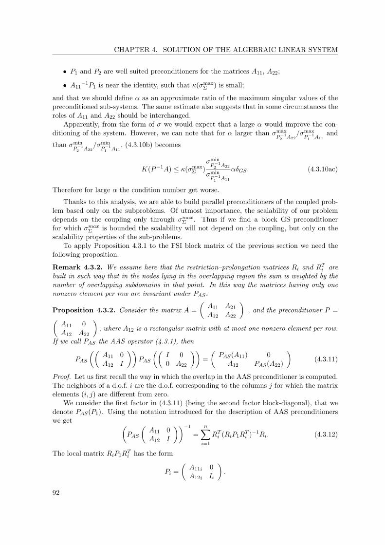
CHAPTER 4. SOLUTION OF THE ALGEBRAIC LINEAR SYSTEM
• P1 and P2 are well suited preconditioners for the matrices A11, A22;
• A11−1P1 is near the identity, such that κ(σmax
Σ ) is small;
and that we should define α as an approximate ratio of the maximum singular values of thepreconditioned sub-systems. The same estimate also suggests that in some circumstances theroles of A11 and A22 should be interchanged.
Apparently, from the form of σ we would expect that a large α would improve the con-ditioning of the system. However, we can note that for α larger than σmax
P−12 A22
/σmaxP−1
1 A11and
than σminP−1
2 A22/σmin
P−11 A11
, (4.3.10b) becomes
K(P−1A) ≤ κ(σmaxΣ )
σminP−1
2 A22
σminP−1
1 A11
αδGS . (4.3.10ac)
Therefore for large α the condition number get worse.
Thanks to this analysis, we are able to build parallel preconditioners of the coupled prob-lem based only on the subproblems. Of utmost importance, the scalability of our problemdepends on the coupling only through σmaxΣ . Thus if we find a block GS preconditionerfor which σmaxΣ is bounded the scalability will not depend on the coupling, but only on thescalability properties of the sub-problems.
To apply Proposition 4.3.1 to the FSI block matrix of the previous section we need thefollowing proposition.
Remark 4.3.2. We assume here that the restriction–prolongation matrices Ri and RTi arebuilt in such way that in the nodes lying in the overlapping region the sum is weighted by thenumber of overlapping subdomains in that point. In this way the matrices having only onenonzero element per row are invariant under PAS.
Proposition 4.3.2. Consider the matrix A =(A11 A21
A12 A22
), and the preconditioner P =(
A11 0A12 A22
), where A12 is a rectangular matrix with at most one nonzero element per row.
If we call PAS the AAS operator (4.3.1), then
PAS
((A11 0A12 I
))PAS
((I 00 A22
))=(PAS(A11) 0A12 PAS(A22)
)(4.3.11)
Proof. Let us first recall the way in which the overlap in the AAS preconditioner is computed.The neighbors of a d.o.f. i are the d.o.f. corresponding to the columns j for which the matrixelements (i, j) are different from zero.
We consider the first factor in (4.3.11) (being the second factor block-diagonal), that wedenote PAS(P1). Using the notation introduced for the description of AAS preconditionerswe get (
PAS
(A11 0A12 I
))−1
=n∑i=1
RTi (RiP1RTi )−1Ri. (4.3.12)
The local matrix RiP1RTi has the form
Pi =(A11i 0A12i Ii
).
92
4.3. PARALLEL PRECONDITIONERS FOR FSI
We can formally write its inverse
P−1i =
(A11
−1i 0
−A12iA11−1i Ii
)=(A11
−1i 0
0 0
)+(
0 0−A12iA11
−1i 0
)+(
0 00 Ii
).
Thus we can rewrite (4.3.12) as (PAS
(A11 0A12 I
))−1
=
n∑i=1
RTi
(A11
−1i 0
0 0
)Ri +
n∑i=1
RTi
(0 0
−A12iA11−1i 0
)Ri +
n∑i=1
RTi
(0 00 Ii
)Ri.
Notice that due to the fact that A12 has at most one nonzero per row
n∑i=1
RTi
(0 0
−A12iA11−1i 0
)Ri =
n∑i=1
RTi
(0 0
−A12i 0
)RiR
Ti
(0 00 A11
−1i
)Ri =
=n∑i=1
(0 0−A12 0
)RTi
(0 00 A11
−1i
)Ri.
This leads eventually to(PAS
(A11 0A12 I
))−1
=(
P−1AS (A11) 0
−A12P−1AS (A11) I
)=(PAS(A11) 0A12 I
)−1
.
From the last identity we have that
PAS
((A11 0A12 I
))=(PAS(A11) 0A12 I
).
Substituting in (4.3.11) we obtain the thesis.
93

Part III
Applications and Simulations


Applications to Hemodynamics
In this chapter we focus on the main application driving our development of the FSI solversdescribed in the previous chapters and developed in the C++ finite element library LifeV8.Our aim is to simulate blood flow in large compliant arteries under both physiological andpathological conditions.
In Section §5.1 we give a brief description of the circulation and of the most common car-diovascular diseases with their possible treatments. In Section §5.2 we give some motivationsand references for the study of FSI in arterial networks and we describe the pipeline usedto obtain FSI simulations from medical raw data. In Section §5.3 we illustrate different ap-proaches to obtain a high quality mesh, we emphasize the importance of building a boundarylayer mesh to obtain accurate values for the wall shear stress even with coarse meshes, andwe report a simulation of blood flow in a femoropopliteal bypass. In Section §5.4 we describea physiological FSI simulation of blood flow in the aortic arch. The choice of appropriateboundary conditions and the effect of modelling the compliance of the arterial wall are dis-cussed. Different methods to solve the nonlinearity and different kinds of time discretizationsdescribed in Part II are compared in Section §5.5.
5.1 Applications and Motivation
The goal of this PhD work is the simulation of blood flow in large arteries. For reader’sconvenience, in this section we briefly summarize the basic elements of blood circulation andthe principal pathologies related to it. We also give a short account on the mathematicalmodeling and the associated results that could be obtained by means of our simulations.
In this description of the human circulatory system, cardiovascular diseases and theirtreatment, we mainly refer to Thiriet [FQV09, Ch.1] and Olufsen et al. [OOL04, Ch.2].
5.1.1 Circulation
The cardiovascular system consists of two parallel circulations: the systemic and pulmonaryones. The systemic arteries transport the oxygenated blood and nutrients toward all thebody, the blood exchanges the oxygen through the capillary networks and returns to theright atrium through the venous system. The pulmonary arteries transport the deoxygenatedblood from the right ventricle to the lungs, there the blood exchanges carbon dioxide withoxygen and returns back to the left atrium through the pulmonary veins. A schematic picturerepresenting systemic and pulmonary circulations is reported in Figure 5.19. The arterial walls
8http://www.lifev.org9Image from http://www.tutorvista.com/biology/systemic-circulation-diagram.

CHAPTER 5. APPLICATIONS TO HEMODYNAMICS
of the pulmonary arteries and veins are much thinner than in the systemic circulation, dueto the lower pressure in the pulmonary circulation. In the following description we focus onthe systemic circulation.
The arteries are in general classified into three categories, although this distinction issometimes not evident. The first category is the one of large arteries, from approximatively2.5 cm of diameter down to 0.1 cm. These arteries are characterized by an elastic behaviourof the wall, whose thickness to diameter ratio is approximately constant and whose Youngmodulus slightly increases when moving distally. The large arteries wall is composed by threelayers: intima, a layer containing the endothelial cells which sense and react to the normal andshear stress coming from the fluid; media, a thick elastic layer composed mainly of elastin andcollagen fibers and of a variable amount of smooth muscle cells; adventitia, a loose externallayer of variable thickness which does not contribute much to the compliance of the wall.Often the boundary between the adventitia and the tissue surrounding the artery is not welldefined.
The second category is the one of arterioles, which play a fundamental role in the cardio-vascular regulation. In this case although the thickness of the wall decreases with the arterydiameter, the thickness to diameter ratio is not constant any more, but it increases when ves-sels become smaller. The walls of the arterioles is almost rigid and it contains smooth musclecells. The presence of these muscle cells allows the arterioles to regulate the intraluminalpressure and radius, in order to meet the needs of the tissue.
The third category of arteries consists of the capillaries. These arteries are very small (fewµm), their wall is composed only by an endothelial cells layer, so that nutrient, oxygen andcarbon dioxide can be exchanged with the interstitial fluid of the tissue cells. The blood flowat the capillary level is not pulsatile any more: the compliance of the arterial wall has theeffect of damping the pulsation of the heart. While the large arteries and arterioles alwaysbifurcate in two, the capillaries can have complicated patterns and bifurcations, also featuringclosed rings.
The flow in the veins is not pulsatile, the pressure is lower than in both systemic andpulmonary circulations. The venous wall is thinner than the arterial one, and valves may bepresent, in order to prevent the flow to go in the wrong direction when the vessel is compressedby a muscle contraction.
Blood is composed mainly by red blood cells (erythrocytes, whose concentration, or hema-tocrit, ranges from 40 to 45%) and plasma (composed for the 98% of water). The red bloodcells have an elastic behaviour, thanks to a cytoskeleton, and can deform when passing throughthe capillaries10. The behaviour of blood is found to be non Newtonian, since the viscositydepends on the shear. The reason is this that when the shear is low the red blood cells tendto interact, increasing the macroscopic viscosity of blood (the shear thinning effect). For highshear (higher than about 1 s−1) there is no interaction and the viscosity of blood in large ar-teries is approximately constant (around 0.03 g/(cm·s) and 0.04 g/(cm·s)). However, also for highshear, the viscosity is found experimentally to drop when the radius of the vessel is smallerthan 0.1 cm.
For these and other reasons the macroscopic modeling of blood flow as a Newtonian fluidand of the arterial wall as an elastic structure is justified only for large arteries, while thecirculation on arterioles and capillaries should be simulated using other models, accounting
10the study of the deformations of the single red blood cells has many medical applications and is subjectof research in microfluidics.
98

5.1. APPLICATIONS AND MOTIVATION
Figure 5.1: Systemic and pulmonary circulation.
Figure 5.2: Atherosclerosis.
for the aforementioned effects. The circulation in the arterioles and capillaries is often calledperipheral circulation, and a proper model describing it in detail should take into accountthe meso and micro scales. If the main focus is on the large arteries simulation, then theperipheral circulation can be accounted for using reduced order models, cf. Section §2.9.
5.1.2 Cardiovascular Diseases
We resume in the following the main cardiovascular diseases with their possible treatment, inorder to show how numerical simulations of such pathological situations can potentially helpmedical doctors in the decision making process. The main cardiovascular diseases affectinglarge arteries are the following:
• Congenital defects, such as bi-leaflet aortic valve, heart septal defects, pulmonary ortricuspid atresia. These defects often require surgical intervention (e.g. the Fontanprocedure for pulmonary or tricuspid atresia [FB71]), in this case numerical simulations
99

CHAPTER 5. APPLICATIONS TO HEMODYNAMICS
Figure 5.3: Saccular and fusiform aneurysms.
can give a prediction of the hemodynamic features (pressure, flow rate, etc.) pre andpost intervention.
• Atherosclerosis, i.e., the accumulation of fatty materials, fibrous elements and calciumon the inner surface of the arterial wall, see Figure 5.211. The formation of atheroscle-rotic plaques generates a stenosis, and at a late stage can provoke a total stenosis of theartery. Furthermore thrombi can detach from the plaque and lead to infarctions andstrokes. Stenosed arteries are in general treated by grafting or stenting, or by removingthe plaque. The first method consists in substituting (or bypassing) the stenosed arteryusing another vessel and creating artificial anastomoses. The second method consists indilating the arterial wall using a balloon and in inserting a device (stent) which supportsthe vessel walls, preserving the original lumen. The main problem of this approach isthe potential restenosis, which can be limited adopting drug eluting stents inhibiting thecells proliferation in the stented region. Experimental evidence suggests that the wallshear stress is involved in the formation of atherosclerotic plaques. Thus a numericalsimulation and a wall shear stress evaluation can help in identifying which locations aremore at risk or to choose an optimal strategy for the surgical interventions.
• Aneurysms, i.e., a dilation of an arterial segment. The vessel wall of an aneurysm ismuch thinner and stiffer than in the physiological case, the collagene fibers being mainresponsible of the mechanic response. The aneurism rupture causes possibly lethalhaemorrages. The aneurysms can be either fusiform or saccular (see Figure 5.312).The main strategies for the treatment of saccular aneurysms are cutting them with asurgical intervention (clipping), or filling them with thin metallic coils, so that mostof the aneurysmal cavity is excluded from the circulation. Fusiform aneurysms areusually treated by grafting, or by using external or internal stents. All these treatmentscould largely benefit from numerical simulations, whose prediction can avoid issues likerecanalisation.
11Image from A.D.A.M., Inc.12Image from http://www.daviddarling.info/encyclopedia/A/aneurysm.html.
100

5.2. PROBLEM DESCRIPTION
Figure 5.4: Ventricular assisted device.
• Heart failure. Implantation of ventricular assisted devices is a reliable treatment forpatients with terminal heart failure. These devices are used as a bridge to transplan-tation, bridge to recovery or destination therapy (for patients who are not eligible forheart transplantation). It consists of an extracorporeal circulation device used to by-pass the left ventricle and to pump the oxygenated blood directly into the aorta seeFigure 5.413. Frequently the hemodynamic modifications due to this treatment lead tocomplications that can be investigated using numerical simulations.
5.2 Problem Description
Blood flow dynamics and arterial wall mechanics are thought to be an important factorin the pathogenesis and treatment of cardiovascular diseases. Indeed more and more databecome available in clinical routine and, at the same time, numerical methods are also moreefficient and capable of reproducing in silico complex phenomena. A number of specifichemodynamic and vascular mechanic factors – notably wall shear stress (WSS), pressure andmural stress, flow rate, and residence time – are implicated in aneurysm growth and rupture[BT96, SD00] or in the pathogenesis of atherosclerosis [KWO+97]. Judicious control of thesehemodynamic factors may also govern the outcomes of vascular therapies [GCF94, GSP92].Computational fluid dynamics and computational fluid structure interaction provide a viableoption for understanding the complex nature of blood flow and arterial wall mechanics and forobtaining those relevant quantities. A better understanding of the hemodynamics could thusimprove the prediction and diagnosis in both healthy and pathological situations [FQV09,Chap. 1]. A simulation with rigid walls fails to predict some essential characteristics of theblood flow (such as pressure wave propagation). Thus it cannot be considered reliable in manysituations (e.g. when the vessels undergo relatively large displacements). However consideringthe full 3D FSI problem increases the computational cost, thus it is of utmost importance todevelop and implement parallel and scalable computational algorithms.
13Image from Wikipedia http://en.wikipedia.org/wiki/Ventricular_assist_device.
101

CHAPTER 5. APPLICATIONS TO HEMODYNAMICS
Modeling the fluid–structure interaction between the blood and the arterial wall is achallenging task. The research in this field is developing fast concerning both the modelingaspects and computational efficiency. Taking into account the compliance of the vessels can beachieved by introducing a 3D or 2D elastic structure, using a Lagrangian (see e.g. [IOP03]),Eulerian (e.g. [CMM08]), or Arbitrary Lagrangian Eulerian formulation (e.g. [SH07], cf.Chapter 1, in [PR95] this approach was pioneered for hemodynamic applications). The struc-ture model should take into account the nonlinearity due to the collagen activation and thepresence of surrounding tissue inducing a static pressure and a dynamic response to the walldisplacement. While in many contexts the rheological properties of blood flow have a greatinfluence on its dynamics, the flow in large healthy arteries is known to have an almostNewtonian behavior [FQV09, OOL04].
Alternative options that avoid the introduction of a structure model for the external wallare transpiration techniques (e.g. [FFT00, DFF03]), the coupled momentum method, usede.g. by Kim et al. [KVCF+09], or other similar approaches (e.g Nobile et al. [NV08]). Thesemethods consist of dropping the non-slip Dirichlet condition at the fluid–structure interface,and substituting it with a proper condition that emulates the presence of a surrounding struc-ture. In particular the coupled momentum method shows good results in many physiologicalsituations, and it has the advantage of being computationally cheap because the mesh isfixed. However, although it is well suited for small displacements, this method can be inap-propriate when the displacements become large [FVCJ+06]. Furthermore, as the fixed controlvolume where the fluid equations are solved allows the fluid to pass through the interface, thequantities computed at the boundary, such as the wall shear stress, are subject to a furtherapproximation.
Thus numerical simulations can help to predict the WSS distribution in a specific geometryof the vessel, improving diagnosis and prevention. A reliable numerical tool that carries outall the process from the patient-specific segmentation to the simulation could help a medicaldoctor, e.g. to identify the regions at risk for pathologies such as atherosclerosis, infarction oraneurisms development [FQV09, Ch. 1]. Furthermore, if the model is validated, a simulationof the WSS distribution can help to solve the inverse problem, i.e., to identify the role thatWSS plays in the development of pathologies such as atherosclerosis.
The numerical computations require meshes describing the patient-specific three-dimensionalcardiovascular geometry. This geometry needs to be reconstructed from medical images, asexplained in the next section.
5.2.1 From DICOM Images to Numerical Simulations
We describe here the set of tools used to build a complete pipeline from raw medical imagesto FSI simulations. A standard file format for medical images data from e.g. CT scans orMRI is the DICOM format. These images can be handled by many open source softwaresfor visualization (see e.g. OsiriX14) or segmentation (see 3D Slicer15 or vmtk16). Althoughsome of these softwares provide advanced tools to detect, extract and smoothen the surfacesof the different organs visible in the raw image, the segmentation step cannot be completelyautomatic due to the noise present in the images which often produces artifacts that have tobe manually removed.
14http://www.osirix-viewer.com/AboutOsiriX.html15http://www.slicer.org16http://www.vmtk.org
102

5.2. PROBLEM DESCRIPTION
While the arterial lumen, which is the part of the vessel occupied by the fluid, is usuallyeasy to detect from the medical images, it is much more difficult to accurately extract thevessel wall. For this reason often the geometry of the vessel wall is obtained using empiricalalgebraic relations available from literature (see e.g. Langewouters et al. [Lan82], cf. Sec-tion §5.4) relating the lumen diameter and the vessel wall thickness. However this approachrequires the definition and computation of the vessel radius, and thus of a vessel centerline,which is not trivial for an arbitrary, possibly branching, artery. Some software, like vmtk,can handle this (see e.g. [Ant02] for an explanation of the methodology).
Once the vessel wall geometry is available, the finite elements discretization requires thegeneration of a mesh for both fluid and solid domains. The surface mesh extracted from theraw medical images however is frequently not suitable for FE applications. In these cases asurface remeshing step is required, cf. Section §5.3. Both these steps can be performed usingopen-source softwares, such as Gmsh17.
Once we have built a tetrahedral mesh conforming at the fluid–structure interface wecan use the LifeV library to run the FSI simulation on the patient specific geometry. LifeVis a free C++ parallel finite elements library distributed under LGPL licence, developed atEPFL in Lausanne, at Politecnico di Milano, at Emory University in Atlanta and at INRIA inParis. Most of the preconditioning strategies and the different algorithms for the FSI problemdescribed in this work have been implemented in the LifeV library as part of this researchproject.
We make below some general comments, which are valid for all the simulations of thissection. LifeV is based on Trilinos18, a parallel library written in C++ which among otherfeatures implements some standard preconditioning strategies, iterative and direct solversand it acts as interface for the linear algebra packages (BLAS, Lapack, UMFPACK). Theparallelization is achieved by partitioning the mesh using the ParMETIS library19, so that eachprocessor holds a mesh partition and all the vectors and matrices are distributed accordingly.The parallelization is based on the MPI API. For FSI the fluid and solid geometries arepartitioned independently, and each processor holds one fluid and one solid partition.
In most of the simulations performed the fluid problem is discretized in space using P1-P1 finite elements stabilized with the interior penalty technique described in [PB05]. Thestabilization parameters chosen, cf. Section §2.7.1, are γβ = 1, γdiv = 0.2 and γp = 0.05.The solid and the geometry problems are discretized in space with P1 finite elements. Thediscretization in time is based on the implicit Euler method for the fluid (in its non conser-vative formulation, cf. Chapter 2) and a mid-point second order scheme for the structure (seeChapter 2 or [Nob01, Chap. 4]).
In all of the simulations presented in this chapter, besides the standard Dirichlet or Neu-mann boundary conditions, less standard defective flux conditions are employed. The impo-sition of flux defective boundary conditions is addressed e.g. in [FGNQ02a, FVV08, VV05],see also Section §2.9, in the rigid walls case. It consists of imposing the mean velocity on agiven surface through Lagrange multipliers. The extension to the compliant case is straight-forward, the only difference being the fact that in this case the section where the conditionsare imposed can change in time. A review and an extension of these methods may be foundin Vergara [Ver10].
17http://geuz.org/gmsh18http://trilinos.sandia.gov19http://glaros.dtc.umn.edu/gkhome/metis/parmetis/overview
103

CHAPTER 5. APPLICATIONS TO HEMODYNAMICS
5.2.2 Unsteady Blood Flow in a Compliant Iliac Artery
Here we give a concrete example of the pipeline used in our applications for running patient–specific simulations starting from raw medical data. This process involves several softwaresthat are distributed under a public license, and are constantly updated and improved. Themany different steps can be resumed in the following list:
1. The manual segmentation, i.e., the extraction of the surface of the vessel lumen fromthe medical data (often in DICOM format). This step is perhaps the most critical, sinceit cannot be completely automated. Many tools can help to carry out the segmentationstep, such as vmtk and 3D Slicer. In the current example this step is avoided, since thegeometry of the lumen of an iliac artery was already available from the Simtk website20.
2. The 3D surface extracted is usually composed of triangles. At this stage the meth-ods described in Section §5.3 (see [MCG+11]) can be used to automatically optimizethe surface mesh. In the current example the harmonic map algorithm illustrated inSection §5.3 is employed.
3. The centerlines of the lumen are computed using vmtk. This allows to compute thethickness proportional to the intraluminal radius. The extrusion of the vessel wall meshcan present some critical aspects. In fact an extrusion in the normal outward directionmay generate inconsistent triangles in proximity of a bifurcation. This issue becomeseven more critical when the surface mesh is refined. This situation at present is notdetected or solved automatically by most of the softwares, developers of the librariescited above (vmtk, Gmsh) are currently working to overcome this issue.
4. A grid for the fluid and solid volumes can be generated using Gmsh, optionally addinga boundary layer in the fluid domain (in this particular case the boundary layer is notpresent).
5. Eventually the FSI simulation can be run using LifeV, with all the possibilities con-cerning boundary conditions and problem formulations discussed so far. The boundaryconditions imposed in this case are defective fluxes on all the inlet and outlets, while aRobin condition is applied on the external wall to simulate the effect of a surroundingtissue (see Equation (5.4.1)).
A picture showing the solution at t = 0.2 s is reported in Figure 5.5. The inlet flux imposedwas obtained from a previous simulation of an aortic arch, while the outlet fluxes correspond tothe inlet value weighted accordingly with the area of each outlet surface (without accountingfor the delay due to the travelling pressure wave). This set of boundary conditions is notmeant to be physiological, and this subsection should be intended as a proof of concept,while we leave for the rest of the chapter the discussion about cases of physiological interest,comparisons and validation of the code.
20https://simtk.org
104
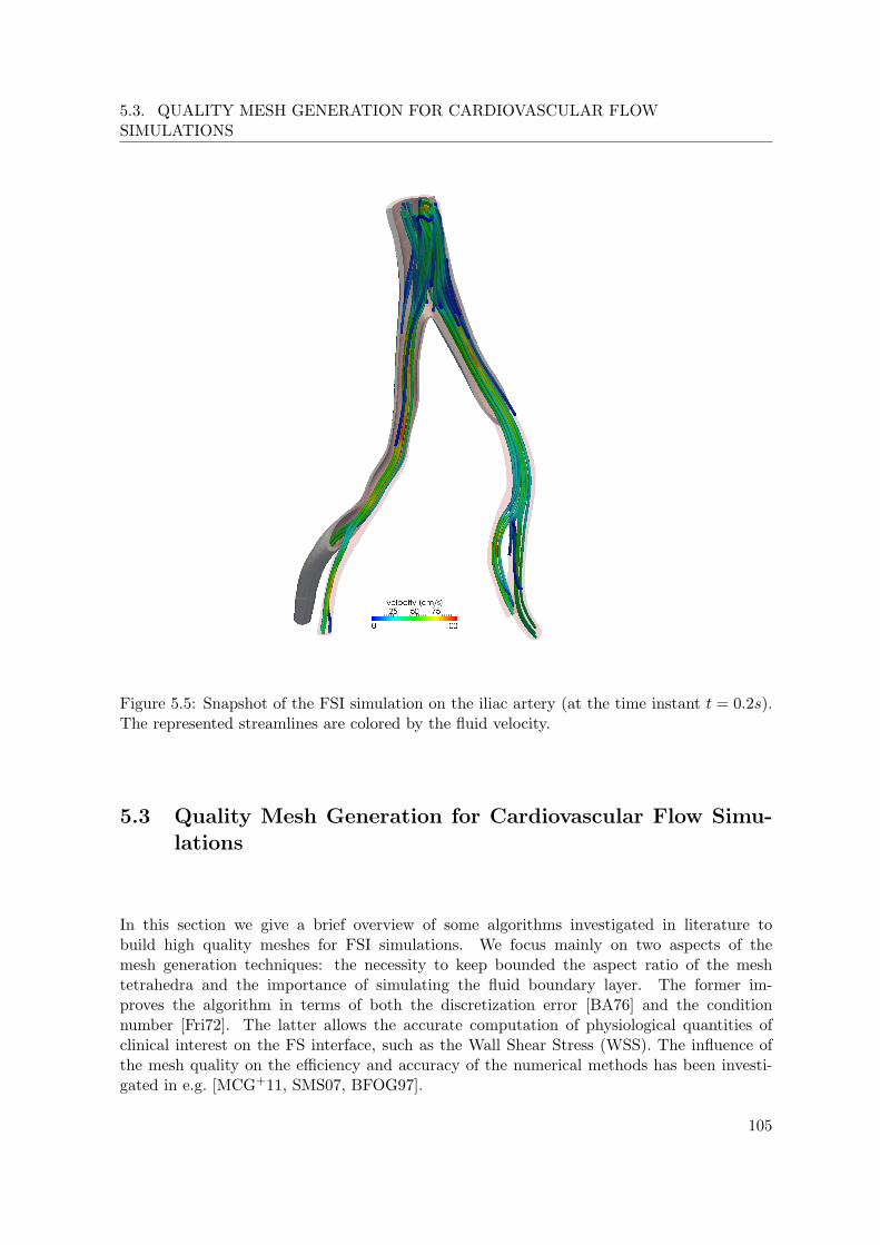
5.3. QUALITY MESH GENERATION FOR CARDIOVASCULAR FLOWSIMULATIONS
Figure 5.5: Snapshot of the FSI simulation on the iliac artery (at the time instant t = 0.2s).The represented streamlines are colored by the fluid velocity.
5.3 Quality Mesh Generation for Cardiovascular Flow Simu-lations
In this section we give a brief overview of some algorithms investigated in literature tobuild high quality meshes for FSI simulations. We focus mainly on two aspects of themesh generation techniques: the necessity to keep bounded the aspect ratio of the meshtetrahedra and the importance of simulating the fluid boundary layer. The former im-proves the algorithm in terms of both the discretization error [BA76] and the conditionnumber [Fri72]. The latter allows the accurate computation of physiological quantities ofclinical interest on the FS interface, such as the Wall Shear Stress (WSS). The influence ofthe mesh quality on the efficiency and accuracy of the numerical methods has been investi-gated in e.g. [MCG+11, SMS07, BFOG97].
105

CHAPTER 5. APPLICATIONS TO HEMODYNAMICS
ξ−1(·)
ξ(·)
Figure 5.6: Map ξ in case of an iliac artery. In this case a portion of the 3D surface is mappedinto a 2D disk to be remeshed.
5.3.1 Surface Remeshing Techniques
From 3D medical images it is usually possible to extract a triangulation of the surface of thevessel. However this surface mesh is often of low quality, oversampled, and featuring verydistorted triangles. A remeshing technique is required for simulation purposes. Furthermoremany algorithms to build meshes in 3D (e.g. Delaunay, Frontal) keep the original surfacemesh on the interface, thus the poor quality of such mesh affects also the quality of the meshinside the 3D domain. The main tools to handle the surface remeshing are
• mesh adaptation strategies [IN02, BCT02, WHMW07],
• meshing techniques that rely on a suitable surface parametrization [BLG00, LB03].
We concentrate here on the second category, referring to [MCG+11] and references therein forfurther details. The idea of the parametrization technique is to optimize a 3D surface meshusing algorithms for the 2D meshes. This is achieved by defining a local frame of referenceon the surface (e.g. as done in Section §1.1), and thus a parametrization ξ(x):
ξ : S ⊂ R3 → S′ ⊂ R2
x 7→ ξ(x)(5.3.1)
that transforms continuously a 3D surface S into a surface S′ embedded in R2.The map ξ is used to pass from the 3D surface to the 2D plane, the remeshing step is
carried out there using a 2D triangulation algorithm and then the mesh is mapped back tothe surface embedded in R3 by means of the inverse of the map ξ. The crucial point of thisstrategy is of course the definition of such a map.
Since our goal is to produce triangular elements as close as possible to equilateral trianglesit is desirable for the map ξ to be conformal, so that the triangles with a good aspect ratioin the 2D mesh are mapped to similar triangles in the surface mesh.
We overview here two methods to build this map which are implemented on the freesoftware Gmsh. One method computes ξ by solving two Laplace equations on the originalsurface triangulation, the other one is based on a least square conformal parametrization ofthe given triangulated surface S.
As shown by Remacle et al. in [RGCM10] and by Marchandise et al. in [MCdWV+10], boththese parameterizations exist if the two surfaces S and S′ have he same topology, e.g. if they
106

5.3. QUALITY MESH GENERATION FOR CARDIOVASCULAR FLOWSIMULATIONS
have zero genus and have at least one boundary. Moreover in order to prevent the numericalissue of indistinguishable coordinates the geometrical aspect ratio should be moderate, whichis often not the case for vascular geometries. In case the topology is wrong and/or if theaspect ratio is too high it can be necessary to call a partitioning algorithm to create differentpatches of correct topology and moderate aspect ratio [MCW+10]. Those patches are thensubsequently remeshed with a finite elements harmonic or least square conformal map.
Harmonic Mapping
We briefly summarize here a method proposed by Remacle et al. [RGCM10] to remesh asurface using harmonic maps. The standard finite elements basis on the surface triangulationis introduced using barycentric coordinates. Two Poisson equations (with proper boundaryconditions) are discretized and solved on the surface mesh for the two coordinate functionsu and v. This allows to build the map ξ in (5.3.1). The map created in this way is the oneminimizing with respect to u and v the quantities
EH(u) =12
∫S‖∇bx(u)‖2 dγ, EH(v) =
12
∫S‖∇bx(v)‖2 dγ. (5.3.2)
The remeshing then takes place in 2D using a standard algorithm. The information about themetric change is taken into account in the remeshing step by the metric tensor G (see Sec-
tion §1.1) associated to the local frame of reference: given that ξ =(uv
), G = (∇ξξ)T∇ξξ
is also the first fundamental form associated to the surface, see [GAS06].
Conformal Mapping
The least square conformal map as introduced by Levy at al. [LPRM02] requires the parametriza-
tion ξ =(uv
)to be such that the gradient of u and the gradient of v are as orthogonal as
possible and have the same norm. For a piecewise linear mapping, the least square conformalmap can be obtained by minimizing the conformal energy:
ELSCM(ξ) =∫
S
12‖∇bxu⊥ −∇bxv‖2ds, (5.3.3)
where ⊥ denotes a counterclockwise 90 rotation in S. For a 3D surface with normal vectorn, the counterclockwise rotation of the gradient can be written as: ∇bxu⊥ = n×∇u.
The form of (5.3.3) is further manipulated and the quadratic minimization problem issolved numerically with finite elements, see [MCG+11] for the details.
5.3.2 High Quality Meshes
Figure 5.7 shows two different steps in the parametrization-based remeshing algorithm of theinitial triangulation of an iliac artery bifurcation. First the initial mesh is cut into differentpatches using the multiscale Laplacian partitioning method described in [MCdWV+10] (Fig-ure 5.7a). Next, each mesh partition (orange and green) is parameterized onto a surface inR2 with a specific mapping algorithm (Figure 5.7bc). We show two different mappings: theLaplacian harmonic map onto a unit disk (Figure 5.7b) and the conformal map with openboundaries (Figure 5.7c).
107
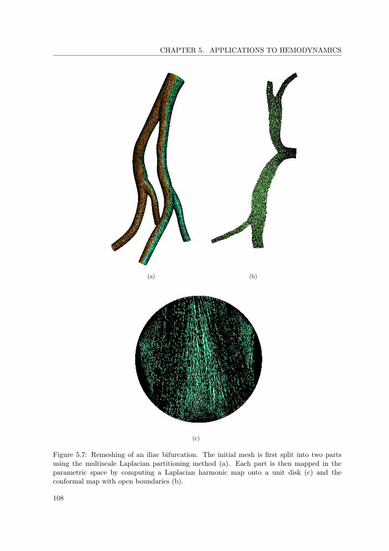
CHAPTER 5. APPLICATIONS TO HEMODYNAMICS
(a) (b)
(c)
Figure 5.7: Remeshing of an iliac bifurcation. The initial mesh is first split into two partsusing the multiscale Laplacian partitioning method (a). Each part is then mapped in theparametric space by computing a Laplacian harmonic map onto a unit disk (c) and theconformal map with open boundaries (b).
108

5.3. QUALITY MESH GENERATION FOR CARDIOVASCULAR FLOWSIMULATIONS
After the mapping has been computed, the parameterized surface is remeshed using a 2Dmesh generation algorithm and the new triangulation is then mapped back to the originalsurface. Figure 5.8 shows part of the remeshed iliac bifurcation for both the harmonic mappingand the conformal map.
(a) (b) (c)
Figure 5.8: Remeshing of an iliac bifurcation: a) part of the initial STL triangulation,b) remeshed geometry with the harmonic mapping using the MeshAdapt meshing algorithm,c) remeshed geometry with the conformal mapping using a frontal 2D meshing algorithm.
109

CHAPTER 5. APPLICATIONS TO HEMODYNAMICS
Inlet
Outlet
Occluded
a) b) c)
Outletpoplitealartery
Occludedfemoralartery bypass
t
Q
Figure 5.9: Segmentation of the arteries of the left lower limb of a patient with a venous graftthat bypasses the occluded femoral artery. We have focused on the geometry of the distalanastomosis. Two different type of meshes are considered for the lumen volume (in red):b) meshes with a viscous boundary layer (BL meshes) and c) fully unstructured tetrahedralmeshes (U meshes). The mesh of the vascular wall is colored in white. The presented meshesare of intermediate mesh size (see Table 5.2).
5.3.3 Unsteady Blood Flow in a Compliant Femoropopliteal Bypass
We compare in this subsection the FSI simulation on different meshes of blood flow in apathological situation. The geometrical model of the distal anastomosis of a femoropoplitealbypass is obtained through a 3T MRI scanner of the left lower limb of a patient. The lumengeometry is subsequently reconstructed in 3D from the raw medical images using the opensource software 3D Slicer21 (see Figure 5.9). The vascular wall is obtained by extruding thelumen surface in the outward normal direction with a wall thickness corresponding to a tenthof the vessel radius. This extruded volume is then composed of 4 layers (the white volume inFigures 5.9b and 5.9c).
For the meshing of the lumen volume (see red volume in Figure 5.9b), we have considereddifferent tetrahedral meshes: three fully unstructured meshes and three meshes with a viscousboundary layer. The size of these meshes is resumed in Table 5.2.
21The bypass geometry was provided by the group of Prof. E. Marchandise, iMCC-MEMA (Universitecatholique de Louvain (UCL)).
110
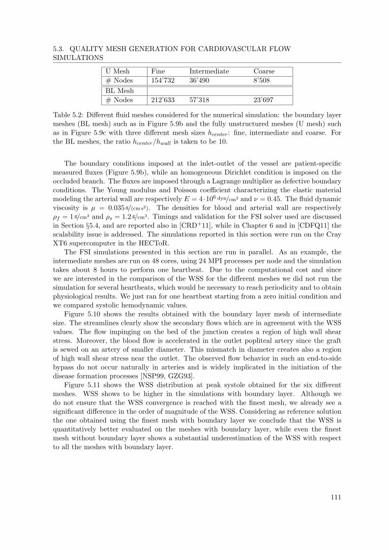
5.3. QUALITY MESH GENERATION FOR CARDIOVASCULAR FLOWSIMULATIONS
U Mesh Fine Intermediate Coarse# Nodes 154’732 36’490 8’508BL Mesh# Nodes 212’633 57’318 23’697
Table 5.2: Different fluid meshes considered for the numerical simulation: the boundary layermeshes (BL mesh) such as in Figure 5.9b and the fully unstructured meshes (U mesh) suchas in Figure 5.9c with three different mesh sizes hcenter: fine, intermediate and coarse. Forthe BL meshes, the ratio hcenter/hwall is taken to be 10.
The boundary conditions imposed at the inlet-outlet of the vessel are patient-specificmeasured fluxes (Figure 5.9b), while an homogeneous Dirichlet condition is imposed on theoccluded branch. The fluxes are imposed through a Lagrange multiplier as defective boundaryconditions. The Young modulus and Poisson coefficient characterizing the elastic materialmodeling the arterial wall are respectively E = 4 ·106 dyn/cm2 and ν = 0.45. The fluid dynamicviscosity is µ = 0.035 g/(cm s2). The densities for blood and arterial wall are respectivelyρf = 1 g/cm3 and ρs = 1.2 g/cm3. Timings and validation for the FSI solver used are discussedin Section §5.4, and are reported also in [CRD+11], while in Chapter 6 and in [CDFQ11] thescalability issue is addressed. The simulations reported in this section were run on the CrayXT6 supercomputer in the HECToR.
The FSI simulations presented in this section are run in parallel. As an example, theintermediate meshes are run on 48 cores, using 24 MPI processes per node and the simulationtakes about 8 hours to perform one heartbeat. Due to the computational cost and sincewe are interested in the comparison of the WSS for the different meshes we did not run thesimulation for several heartbeats, which would be necessary to reach periodicity and to obtainphysiological results. We just ran for one heartbeat starting from a zero initial condition andwe compared systolic hemodynamic values.
Figure 5.10 shows the results obtained with the boundary layer mesh of intermediatesize. The streamlines clearly show the secondary flows which are in agreement with the WSSvalues. The flow impinging on the bed of the junction creates a region of high wall shearstress. Moreover, the blood flow is accelerated in the outlet popliteal artery since the graftis sewed on an artery of smaller diameter. This mismatch in diameter creates also a regionof high wall shear stress near the outlet. The observed flow behavior in such an end-to-sidebypass do not occur naturally in arteries and is widely implicated in the initiation of thedisease formation processes [NSP99, GZG93].
Figure 5.11 shows the WSS distribution at peak systole obtained for the six differentmeshes. WSS shows to be higher in the simulations with boundary layer. Although wedo not ensure that the WSS convergence is reached with the finest mesh, we already see asignificant difference in the order of magnitude of the WSS. Considering as reference solutionthe one obtained using the finest mesh with boundary layer we conclude that the WSS isquantitatively better evaluated on the meshes with boundary layer, while even the finestmesh without boundary layer shows a substantial underestimation of the WSS with respectto all the meshes with boundary layer.
111
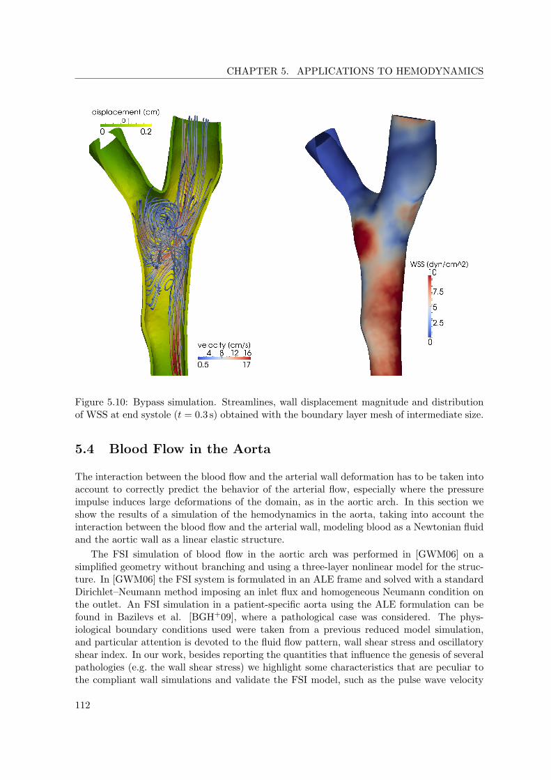
CHAPTER 5. APPLICATIONS TO HEMODYNAMICS
Figure 5.10: Bypass simulation. Streamlines, wall displacement magnitude and distributionof WSS at end systole (t = 0.3 s) obtained with the boundary layer mesh of intermediate size.
5.4 Blood Flow in the Aorta
The interaction between the blood flow and the arterial wall deformation has to be taken intoaccount to correctly predict the behavior of the arterial flow, especially where the pressureimpulse induces large deformations of the domain, as in the aortic arch. In this section weshow the results of a simulation of the hemodynamics in the aorta, taking into account theinteraction between the blood flow and the arterial wall, modeling blood as a Newtonian fluidand the aortic wall as a linear elastic structure.
The FSI simulation of blood flow in the aortic arch was performed in [GWM06] on asimplified geometry without branching and using a three-layer nonlinear model for the struc-ture. In [GWM06] the FSI system is formulated in an ALE frame and solved with a standardDirichlet–Neumann method imposing an inlet flux and homogeneous Neumann condition onthe outlet. An FSI simulation in a patient-specific aorta using the ALE formulation can befound in Bazilevs et al. [BGH+09], where a pathological case was considered. The phys-iological boundary conditions used were taken from a previous reduced model simulation,and particular attention is devoted to the fluid flow pattern, wall shear stress and oscillatoryshear index. In our work, besides reporting the quantities that influence the genesis of severalpathologies (e.g. the wall shear stress) we highlight some characteristics that are peculiar tothe compliant wall simulations and validate the FSI model, such as the pulse wave velocity
112
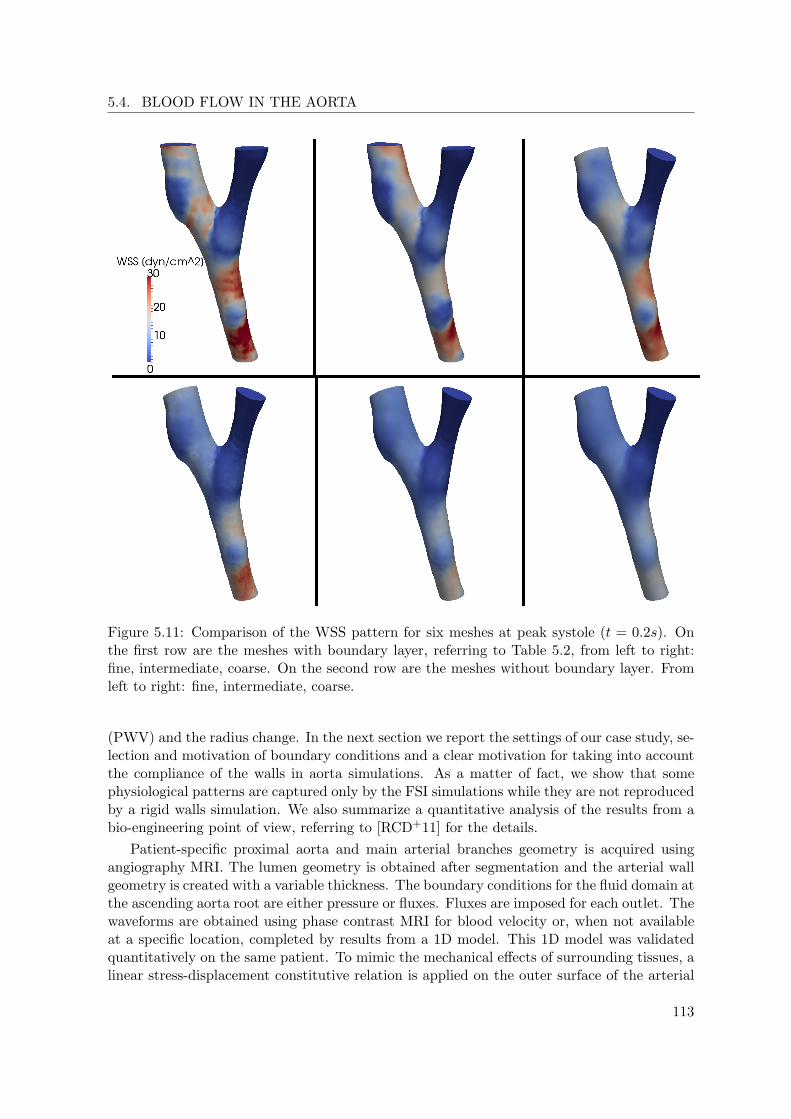
5.4. BLOOD FLOW IN THE AORTA
Figure 5.11: Comparison of the WSS pattern for six meshes at peak systole (t = 0.2s). Onthe first row are the meshes with boundary layer, referring to Table 5.2, from left to right:fine, intermediate, coarse. On the second row are the meshes without boundary layer. Fromleft to right: fine, intermediate, coarse.
(PWV) and the radius change. In the next section we report the settings of our case study, se-lection and motivation of boundary conditions and a clear motivation for taking into accountthe compliance of the walls in aorta simulations. As a matter of fact, we show that somephysiological patterns are captured only by the FSI simulations while they are not reproducedby a rigid walls simulation. We also summarize a quantitative analysis of the results from abio-engineering point of view, referring to [RCD+11] for the details.
Patient-specific proximal aorta and main arterial branches geometry is acquired usingangiography MRI. The lumen geometry is obtained after segmentation and the arterial wallgeometry is created with a variable thickness. The boundary conditions for the fluid domain atthe ascending aorta root are either pressure or fluxes. Fluxes are imposed for each outlet. Thewaveforms are obtained using phase contrast MRI for blood velocity or, when not availableat a specific location, completed by results from a 1D model. This 1D model was validatedquantitatively on the same patient. To mimic the mechanical effects of surrounding tissues, alinear stress-displacement constitutive relation is applied on the outer surface of the arterial
113

CHAPTER 5. APPLICATIONS TO HEMODYNAMICS
wall. This is imposed as a Robin condition, as explained in the next subsection.
5.4.1 Boundary Conditions
When dealing with sectors of vascular districts, the boundary conditions for the numericalsimulation play an important role. For instance they allow to take into account the globalcirculation and the presence of surrounding tissue. The former mainly affects the fluid flow,the latter the structure displacement.
A crucial issue concerning the imposition of boundary conditions on the arterial wall isthe choice of the conditions for the terminations of the arterial branches. On the fluid outletsfluxes obtained by a 1D tree simulation are imposed by Lagrange multipliers as describedin [Ver10, FGNQ02a]. At the inlet, i.e., at the aortic valve location, we impose either theflux measured on the patient or a pressure obtained from the 1D simulation. Here we do notaccount for the coupling between the 3D simulation and the 1D one.
Another possibility currently under development is to model the interaction between thesegment of aorta considered and the rest of the circulation through the geometrical multiscaleframework introduced in Section §2.9. In this way the morphology of the arterial tree and theperipheral circulation can be taken into account. Another simpler option which models thecontinuation of the artery segments at their boundary, and account for the resistance to theflow due to an hydrostatic pressure, consists in absorbing boundary conditions (a particulartype of 0D models), also recalled in Section §2.9. However such conditions on the fluid outletsinhibit the imposition of other physiological quantities such as velocity or stress and emulatesthe continuation of the vessel with an infinite long cylinder.
In literature many strategies to impose absorbing boundary conditions on the fluid outletshave been devised. These allow in FSI to avoid the non physiological pressure wave reflections[Nob01, FQV09, KVCF+09], cf. Section §2.9.
The 1D tree model and the simulation used to impose these boundary conditions aredetailed in [RBP+10]. Each piece of the tree is a one-dimensional reduction of the FSIproblem (cf. Section §2.9). The main systemic arteries as well as a detailed description of thecerebral circulation are represented. The constitutive law for the arterial wall is non-linearand viscoelastic.
This has been validated qualitatively and quantitatively on the same person [RBP+10].Pressure was measured with applanation tonometry22 and cerebral blood flow velocities withtranscranial ultrasound and phase contrast MRI. Pressure and fluxes were computed at eachsegment of the arterial tree. The mean fluxes at each inlet and outlets are summarized inTable 5.3, and the history of the fluxes is shown in Figure 5.12.
Concerning the structure, at the best of our knowledge absorbing boundary conditions forFSI have not been implemented yet, thus we chose in our simulations to clamp the vessel wallat the aortic valve and to impose a Neumann homogeneous condition on the structure outflowterminations. With this choice we did not observe spurious reflection waves. A possible (morephysiological) option would be to adopt the same strategy as for the fluid, that is to imposethe displacement obtained from the previous 1D simulation (cf. Remark 2.9.1).
The simulation of a vessel subject to a high load, as it is the case in the thoracic aorta,undergoes large deformations concerning both the luminal radius and the vessel displacement.
22A non-invasive technique for assessing cardiovascular function. Applanation tonometry is frequently usedto measure pulse wave velocity and to perform pulse wave analysis pulse wave analysis[TY01]
114

5.4. BLOOD FLOW IN THE AORTA
0
50
100
150
200
250
300
350
400
0 0.1 0.2 0.3 0.4 0.5 0.6 0.7 0.8
Flu
x [cm
3/s
]
time [s]
Aortic valve
-10
-5
0
5
10
15
20
25
30
0 0.1 0.2 0.3 0.4 0.5 0.6 0.7 0.8
Flu
x [
cm
3/s
]
time [s]
-5
0
5
10
15
20
0 0.1 0.2 0.3 0.4 0.5 0.6 0.7 0.8
Flu
x [cm
3/s
]
time [s]
Left common carotid
0.5
1
1.5
2
2.5
3
0 0.1 0.2 0.3 0.4 0.5 0.6 0.7 0.8
Flu
x [cm
3/s
]
time [s]
Left vertebral
0
5
10
15
20
25
0 0.1 0.2 0.3 0.4 0.5 0.6 0.7 0.8F
lux
[cm
3/s
]
time [s]
-10
-5
0
5
10
15
20
25
0 0.1 0.2 0.3 0.4 0.5 0.6 0.7 0.8
Flu
x [c
m3/s
]
time [s]
Right common carotid
0
1
2
3
4
5
0 0.1 0.2 0.3 0.4 0.5 0.6 0.7 0.8
Flu
x [
cm
3/s
]
time [s]
Right vertebral
0
50
100
150
200
250
0 0.1 0.2 0.3 0.4 0.5 0.6 0.7 0.8
Flu
x [c
m3/s
]
time [s]
Thoracic aorta
Left subclavian
Right subclavian
Figure 5.12: 3D representation of the lumen of the aortic arch and its principal branches.It consists of 1 inlet (ascending aorta root) and 7 outlets (vertebral, subclavian and carotidarteries, and thoracic aorta). The fluxes imposed as boundary conditions are represented foreach inlet-outlet and are the result of a 1D tree simulation.
In particular, in a curved vessel, when imposing a free stress condition on the external wall,the movement of the domain turns out to be overestimated, as the surrounding tissue aroundthe solid wall is not taken into account in the model.
The importance of considering the surrounding tissue effects is often neglected, although
115
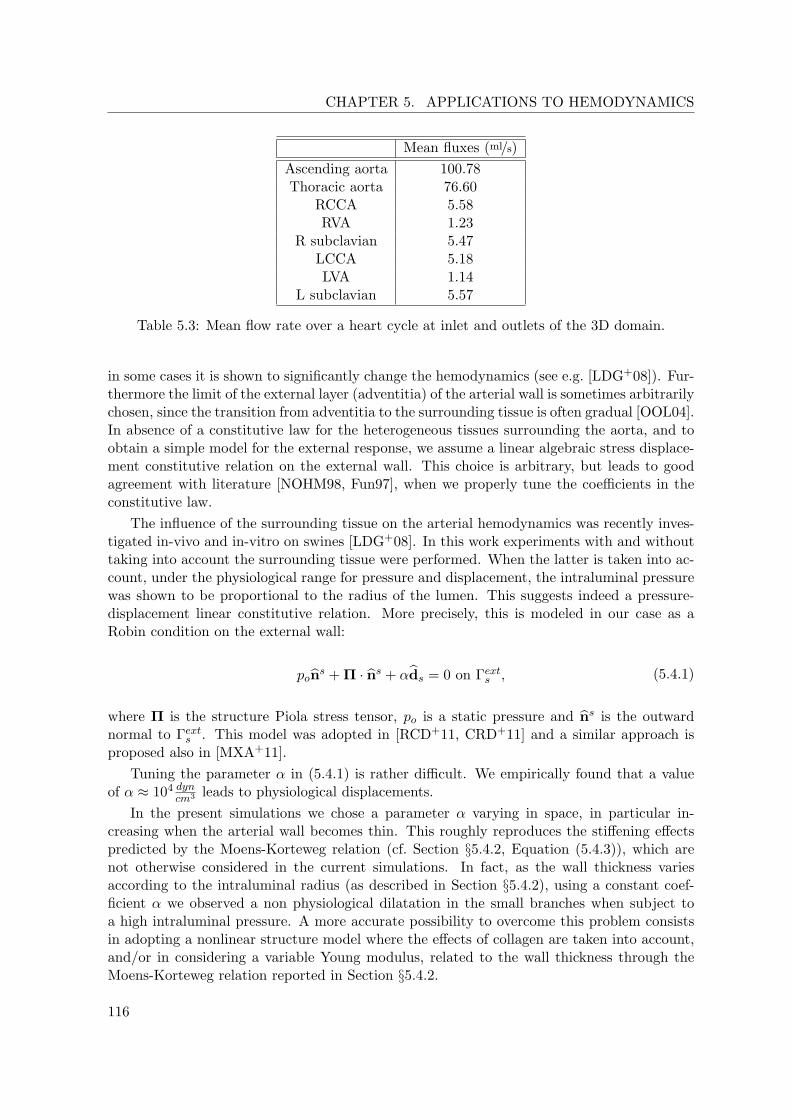
CHAPTER 5. APPLICATIONS TO HEMODYNAMICS
Mean fluxes (ml/s)Ascending aorta 100.78Thoracic aorta 76.60
RCCA 5.58RVA 1.23
R subclavian 5.47LCCA 5.18LVA 1.14
L subclavian 5.57
Table 5.3: Mean flow rate over a heart cycle at inlet and outlets of the 3D domain.
in some cases it is shown to significantly change the hemodynamics (see e.g. [LDG+08]). Fur-thermore the limit of the external layer (adventitia) of the arterial wall is sometimes arbitrarilychosen, since the transition from adventitia to the surrounding tissue is often gradual [OOL04].In absence of a constitutive law for the heterogeneous tissues surrounding the aorta, and toobtain a simple model for the external response, we assume a linear algebraic stress displace-ment constitutive relation on the external wall. This choice is arbitrary, but leads to goodagreement with literature [NOHM98, Fun97], when we properly tune the coefficients in theconstitutive law.
The influence of the surrounding tissue on the arterial hemodynamics was recently inves-tigated in-vivo and in-vitro on swines [LDG+08]. In this work experiments with and withouttaking into account the surrounding tissue were performed. When the latter is taken into ac-count, under the physiological range for pressure and displacement, the intraluminal pressurewas shown to be proportional to the radius of the lumen. This suggests indeed a pressure-displacement linear constitutive relation. More precisely, this is modeled in our case as aRobin condition on the external wall:
pons + Π · ns + αds = 0 on Γexts , (5.4.1)
where Π is the structure Piola stress tensor, po is a static pressure and ns is the outwardnormal to Γexts . This model was adopted in [RCD+11, CRD+11] and a similar approach isproposed also in [MXA+11].
Tuning the parameter α in (5.4.1) is rather difficult. We empirically found that a valueof α ≈ 104 dyn
cm3 leads to physiological displacements.In the present simulations we chose a parameter α varying in space, in particular in-
creasing when the arterial wall becomes thin. This roughly reproduces the stiffening effectspredicted by the Moens-Korteweg relation (cf. Section §5.4.2, Equation (5.4.3)), which arenot otherwise considered in the current simulations. In fact, as the wall thickness variesaccording to the intraluminal radius (as described in Section §5.4.2), using a constant coef-ficient α we observed a non physiological dilatation in the small branches when subject toa high intraluminal pressure. A more accurate possibility to overcome this problem consistsin adopting a nonlinear structure model where the effects of collagen are taken into account,and/or in considering a variable Young modulus, related to the wall thickness through theMoens-Korteweg relation reported in Section §5.4.2.
116

5.4. BLOOD FLOW IN THE AORTA
5.4.2 Geometrical Model
The segmentation and the reconstruction of the arterial wall geometry for the present simula-tion was carried out by Dr. P. Reymond and collaborators (LHTC, EPFL) and it is describedwith more details in [RCD+11]. To obtain a 3D representation of the arterial lumen (inter-face between arterial wall and blood), MRI Time of Flight acquisition on a 3T MRI scanner(Siemens Trio-Tim 3T System) were performed. Details on the sequences utilized are men-tioned in [RBP+10].
The arterial tree geometry was reconstructed in 3D from the raw DICOM medical images(ITK Snap). After pre-processing of the DICOM images, using gradient diffusion, a growingregion based on contrast threshold was obtained. This served as a starting surface for animproved segmentation using an edge detection method based on intensity gradients.
First a geometrical surface of the lumen was created from the extracted surface (thatwas previously segmented) using ICEM CFD 1123. The lumen extracted surface of the aortawas obtained by MRI, however the thickness of the arterial wall was not retrieved with thistechnique. To build the geometry of the solid region in a physiological manner it has beenbased on human ex-vivo measurements carried out by Langewouters et al. [Lan82]. Basedon ex-vivo samples, they performed thickness (h) and outer diameter (De) measurements onhuman thoracic aortas and reported thickness to arterial diameter ratio as a function of ageand location:
h
De= a+ b · age = Const.
The thickness varies spatially and is proportional to the local lumen diameter. The reportedvalue of this ratio is c = 0.054 for the thoracic aorta and c = 0.07 for the abdominal aortafor a 30 years old male. We use the mean value of these two aortic locations for the wholecomputational domain (i.e., we assume that ratio constant). Therefore the thickness to lumendiameter that we assumed for the whole aorta in the model is
h
Dlumen=
c
1− 2c≈ 0.071 (5.4.2)
The lumen diameter (Dlumen) was deduced from the local distance between vessel centerlineand arterial lumen mesh elements. The thickness was set locally in the normal direction, itvaries spatially and decreases when moving downstream.
The centerline of the arterial tree was computed using the Aneufuse software developed bythe EU Project @neurIST. An unstructured tetrahedral mesh, conforming at the FS interface,was then generated for the fluid region using Gambit24.
Although the procedure for extracting the vessel wall thickness is not arbitrary, a certainvariability is expected, due e.g. to the difference between the ex-vivo and the in-vivo measures.Furthermore the following components that describe the geometry and the stiffness of thearterial wall are function of the location:
• the elastic modulus of the arterial wall increases when moving distally (constituents ofthe arterial wall, elastin/collagen repartition is different)
• the arterial diameter to thickness ratio increases as well when moving distally.23ANSYS Inc., Canonsburg, PA24ANSYS Inc., Canonsburg, PA
117

CHAPTER 5. APPLICATIONS TO HEMODYNAMICS
Figure 5.13: Arterial wall cut representation. The mesh has a variable thickness, proportionalto the local lumen diameter of the vessel. In this example, the mesh contains 3 layers ofprismatic elements, which are later replaced by tetrahedral elements in order to be compatiblewith the LifeV solver.
The contribution of these two components increases the pulse wave velocity, a clinical parame-ter of importance, which has been shown, in-vivo, to increase as well when moving distally. Infact according to the adapted Moens-Korteweg equation, the relationship between the elasticmodulus ε and the pulse wave velocity PWV [NO05] is given by:
PWV =
√εh
νD(1− ν2), (5.4.3)
where ν is the Poisson coefficient of the arterial wall (ν = 0.45). We obtained a PWV that isapproximatively 5 m/s. It corresponds to physiological data for a young person aorta.
The arterial wall constitutive relation in our case is linear elastic and isotropic. Thisis quite a restrictive assumption and the generalization to nonlinear elasticity is subject ofongoing work. However for a simulation of non-pathological range of intra arterial pressuresit leads to results in the physiological range of values; as we will show (cf. Section §5.5),these results by far improve those obtained using the rigid walls assumption. In this study weassume also that the thickness to arterial lumen diameter ratio h/D and the elastic modulus(ε = 0.4 MPa) for the whole geometry of the arterial wall are constant. In a similar study, byKim et al. [KVCF+09], a constant value of ε = 0.6 MPa was used. Due to the observationsabove the assumption of constant Young modulus becomes less physiologically accurate whenconsidering an extended region of the cardiovascular system.
The increase in the coefficient α in (5.4.1) contributes to stiffen the arterial wall whenmoving distally, which mimics the effects described above.
5.4.3 Timings and Validation for FSI (GCE)
The FSI simulations are run for three heartbeats, Figure 5.14 reports the pressure and dis-placement for fixed time steps. There are no significant differences in the time history ofpressures and fluxes between the second and the third heartbeat (Figures 5.16 and 5.17),which suggests that the solution reached a substantial periodicity.
These simulations are performed using the GCE time discretization, cf. Section §2.6. Othertime discretizations are explored in Section §5.5, which are more reliable but more computa-
118

5.4. BLOOD FLOW IN THE AORTA
(a) (b) (c) (d)
(e) (f)
Figure 5.14: Pressure and displacement distribution at different times. Figure (a) representsthe pressure at the end of the second heartbeat (at t = 1.6 s). The pictures (b), (c), (d)are taken at intervals of 0.2 s. We remark that the pressure reaches the maximum value inproximity of the systole, at t ≈ 1.8 s. The (e) and (f) figures represent the displacementmagnitude at t = 1.8 s and t = 2.2 s. The location of the maximum displacement duringsystole in the aortic arch is probably due to the curved and branching shape of the geometryinducing a variation of the eccentricity of the lumen.
tionally expensive. In that section also other comparisons (with a rigid walls simulation andwith a 1D model simulation) are carried out, while in the rest of this section we focus on thedescription of the results of the simulations obtained, in terms of computational efficiencyand of clinical interest of the output.
The results of this subsection are obtained using the Cray XT4 supercomputer in HEC-ToR. These simulations are run on 16 nodes for a total of 64 MPI processes, and the meshconsidered is the one represented in Figure 5.18. For the domain partitioning we used theParMETIS25 library (Figure 5.18 shows the partition of the artery in 32 subdomains). Thepartition of the fluid and solid meshes is performed independently, and each processor holdsboth a fluid and a solid partition.
At every time-step most of the time is spent in the preconditioner computation, in the
25http://glaros.dtc.umn.edu/gkhome/metis/parmetis/overview
119

CHAPTER 5. APPLICATIONS TO HEMODYNAMICS
Figure 5.15: Sections in which the mean values of pressure and velocity are computed.
Figure 5.16: FSI simulation with inlet flux imposed. History of the mean pressures (in mmHg)at S1, S2, S3 and S4 in Figure 5.15 (starting from the left with the S1 section, until the S4
section on the right).
Figure 5.17: FSI simulation with inlet flux imposed. Mean velocities computed in the sectionsS1, S2, S3 and S4 represented in Figure 5.15.
solution of the linear system, and in the assembly of the matrix block corresponding to thefluid equations. The average time for these tasks is 16.6 s, 11.5 s and 8.1 s respectively (theassembly of the stabilization part at every time iteration takes 7.1 s, while the assembly ofthe rest of the block takes about 1 s).
120

5.4. BLOOD FLOW IN THE AORTA
The preconditioner considered is PAS−DN1 (cf. Section §4.3.2), where a one-level algebraicadditive Schwarz (AAS) preconditioner with two layers overlap (see [QV99]) is employed foreach factor. The LU factorization of the sub-blocks in the AAS preconditioner is achievedthrough the unsymmetric multifrontal method implemented in the package UMFPACK26.The linear system is solved with preconditioned GMRES iterations and the average numberof iterations is about 25 to reach a tolerance of 10−7.
The time-step chosen is δt = 10−3 s, so that one heartbeat (0.8 s) consisted of 800 timelevels. Summing the timings for the solution of the linear system, the preconditioner compu-tation and the assembly of the fluid block we obtain a global timing per heartbeat of about8 hours. We remark that the assembly of the fluid block scales when increasing the numberof processors since it requires few inter-processor communications (the ghost nodes of eachpartition are repeated on all the processors), while the preconditioner computation, and inparticular the GMRES solution, are less scalable operations. We refer to [CDFQ11] and toChapter 6 for considerations on the scalability of the FSI system and for a discussion onsuitable preconditioners for coupled problems.
Figure 5.18: Aorta mesh partitioned with 32 processors using ParMETIS. The mesh is com-posed of 380′690 tetrahedra, i.e., 486′749 dofs.. On the right: the fluid mesh partitioned; onthe left: both fluid and solid mesh partitioned.
In order to compare the time spent for one iteration of rigid walls with that spent for aniteration with FSI GCE we run another cycle of 200 time steps for both rigid walls and FSI
26http://www.cise.ufl.edu/research/sparse/umfpack
121
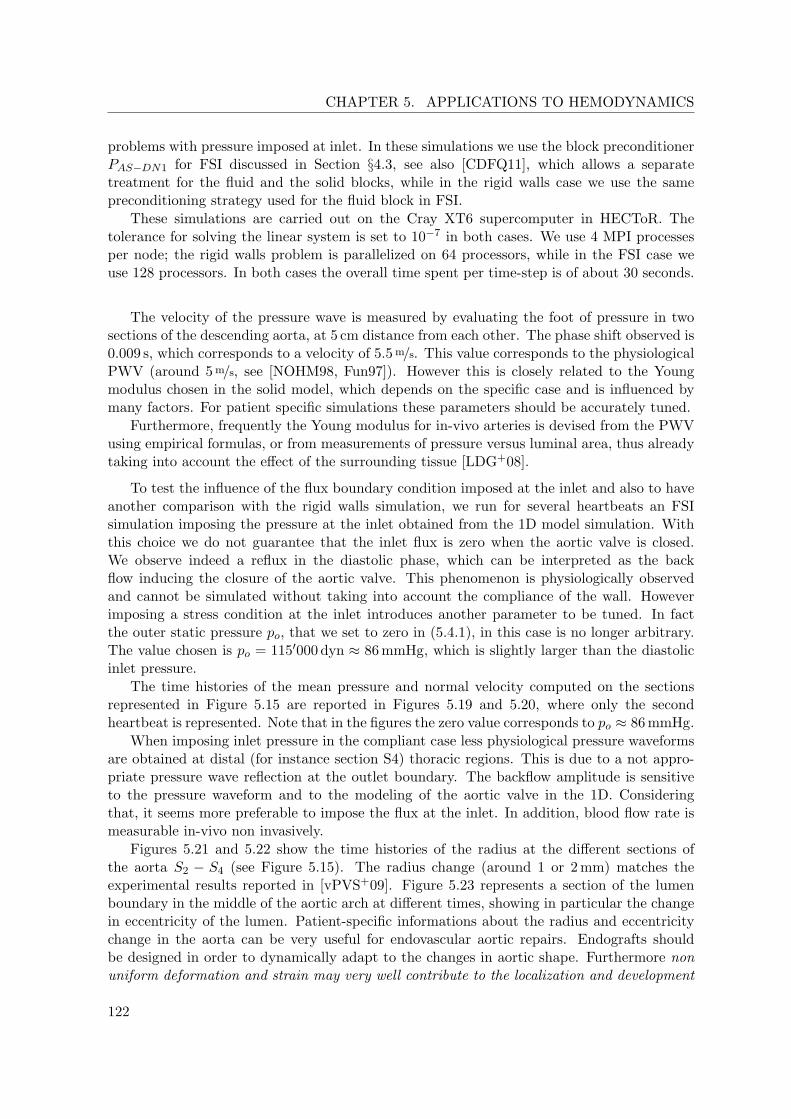
CHAPTER 5. APPLICATIONS TO HEMODYNAMICS
problems with pressure imposed at inlet. In these simulations we use the block preconditionerPAS−DN1 for FSI discussed in Section §4.3, see also [CDFQ11], which allows a separatetreatment for the fluid and the solid blocks, while in the rigid walls case we use the samepreconditioning strategy used for the fluid block in FSI.
These simulations are carried out on the Cray XT6 supercomputer in HECToR. Thetolerance for solving the linear system is set to 10−7 in both cases. We use 4 MPI processesper node; the rigid walls problem is parallelized on 64 processors, while in the FSI case weuse 128 processors. In both cases the overall time spent per time-step is of about 30 seconds.
The velocity of the pressure wave is measured by evaluating the foot of pressure in twosections of the descending aorta, at 5 cm distance from each other. The phase shift observed is0.009 s, which corresponds to a velocity of 5.5 m/s. This value corresponds to the physiologicalPWV (around 5 m/s, see [NOHM98, Fun97]). However this is closely related to the Youngmodulus chosen in the solid model, which depends on the specific case and is influenced bymany factors. For patient specific simulations these parameters should be accurately tuned.
Furthermore, frequently the Young modulus for in-vivo arteries is devised from the PWVusing empirical formulas, or from measurements of pressure versus luminal area, thus alreadytaking into account the effect of the surrounding tissue [LDG+08].
To test the influence of the flux boundary condition imposed at the inlet and also to haveanother comparison with the rigid walls simulation, we run for several heartbeats an FSIsimulation imposing the pressure at the inlet obtained from the 1D model simulation. Withthis choice we do not guarantee that the inlet flux is zero when the aortic valve is closed.We observe indeed a reflux in the diastolic phase, which can be interpreted as the backflow inducing the closure of the aortic valve. This phenomenon is physiologically observedand cannot be simulated without taking into account the compliance of the wall. Howeverimposing a stress condition at the inlet introduces another parameter to be tuned. In factthe outer static pressure po, that we set to zero in (5.4.1), in this case is no longer arbitrary.The value chosen is po = 115′000 dyn ≈ 86 mmHg, which is slightly larger than the diastolicinlet pressure.
The time histories of the mean pressure and normal velocity computed on the sectionsrepresented in Figure 5.15 are reported in Figures 5.19 and 5.20, where only the secondheartbeat is represented. Note that in the figures the zero value corresponds to po ≈ 86 mmHg.
When imposing inlet pressure in the compliant case less physiological pressure waveformsare obtained at distal (for instance section S4) thoracic regions. This is due to a not appro-priate pressure wave reflection at the outlet boundary. The backflow amplitude is sensitiveto the pressure waveform and to the modeling of the aortic valve in the 1D. Consideringthat, it seems more preferable to impose the flux at the inlet. In addition, blood flow rate ismeasurable in-vivo non invasively.
Figures 5.21 and 5.22 show the time histories of the radius at the different sections ofthe aorta S2 − S4 (see Figure 5.15). The radius change (around 1 or 2 mm) matches theexperimental results reported in [vPVS+09]. Figure 5.23 represents a section of the lumenboundary in the middle of the aortic arch at different times, showing in particular the changein eccentricity of the lumen. Patient-specific informations about the radius and eccentricitychange in the aorta can be very useful for endovascular aortic repairs. Endografts shouldbe designed in order to dynamically adapt to the changes in aortic shape. Furthermore nonuniform deformation and strain may very well contribute to the localization and development
122

5.4. BLOOD FLOW IN THE AORTA
of vascular pathology [vPVS+09].
Figure 5.19: FSI simulation with inlet pressure imposed. History of the mean pressures (inmmHg) over the sections S1, S2, S3 and S4 represented in Figure 5.15. The zero value of thepressure correspond to po ≈ 86 mmHg.
Figure 5.20: FSI simulation with inlet pressure imposed. History of the mean normal velocities(in cm/s) over the sections S1, S2, S3 and S4 represented in Figure 5.15. In the plot for theS1 section (left) we show the pressure curve over the same section with a dashed line, tohighlight the dependence of the reverse flow on the steep pressure decrease after the systole.Notice that at regime in the abdominal aorta no more backward flow is observed.
123

CHAPTER 5. APPLICATIONS TO HEMODYNAMICS
Figure 5.21: FSI simulation with inlet flux imposed. History of the mean radius over thesections S2, S3 and S4 represented in Figure 5.15 (third heartbeat).
Figure 5.22: FSI simulation with inlet pressure imposed. History of the mean radius over thesections S2, S3 and S4 represented in Figure 5.15 (third heartbeat).
124
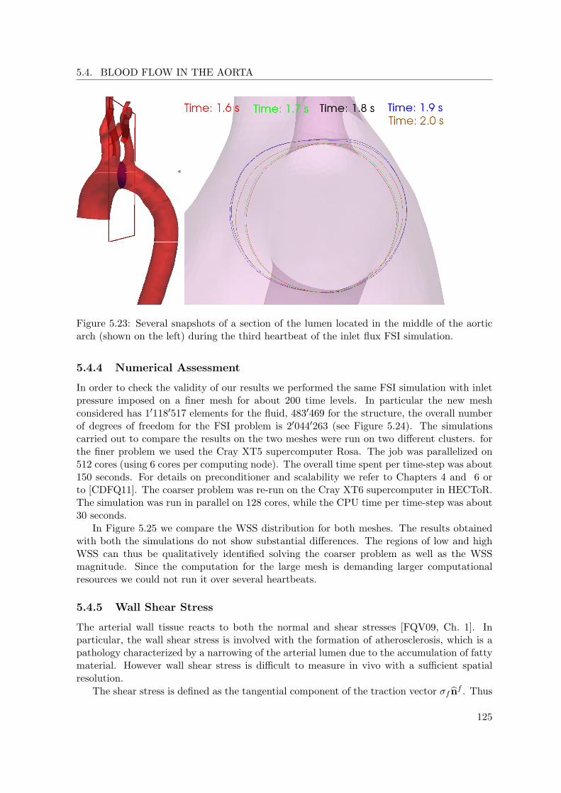
5.4. BLOOD FLOW IN THE AORTA
Figure 5.23: Several snapshots of a section of the lumen located in the middle of the aorticarch (shown on the left) during the third heartbeat of the inlet flux FSI simulation.
5.4.4 Numerical Assessment
In order to check the validity of our results we performed the same FSI simulation with inletpressure imposed on a finer mesh for about 200 time levels. In particular the new meshconsidered has 1′118′517 elements for the fluid, 483′469 for the structure, the overall numberof degrees of freedom for the FSI problem is 2′044′263 (see Figure 5.24). The simulationscarried out to compare the results on the two meshes were run on two different clusters. forthe finer problem we used the Cray XT5 supercomputer Rosa. The job was parallelized on512 cores (using 6 cores per computing node). The overall time spent per time-step was about150 seconds. For details on preconditioner and scalability we refer to Chapters 4 and 6 orto [CDFQ11]. The coarser problem was re-run on the Cray XT6 supercomputer in HECToR.The simulation was run in parallel on 128 cores, while the CPU time per time-step was about30 seconds.
In Figure 5.25 we compare the WSS distribution for both meshes. The results obtainedwith both the simulations do not show substantial differences. The regions of low and highWSS can thus be qualitatively identified solving the coarser problem as well as the WSSmagnitude. Since the computation for the large mesh is demanding larger computationalresources we could not run it over several heartbeats.
5.4.5 Wall Shear Stress
The arterial wall tissue reacts to both the normal and shear stresses [FQV09, Ch. 1]. Inparticular, the wall shear stress is involved with the formation of atherosclerosis, which is apathology characterized by a narrowing of the arterial lumen due to the accumulation of fattymaterial. However wall shear stress is difficult to measure in vivo with a sufficient spatialresolution.
The shear stress is defined as the tangential component of the traction vector σf nf . Thus
125
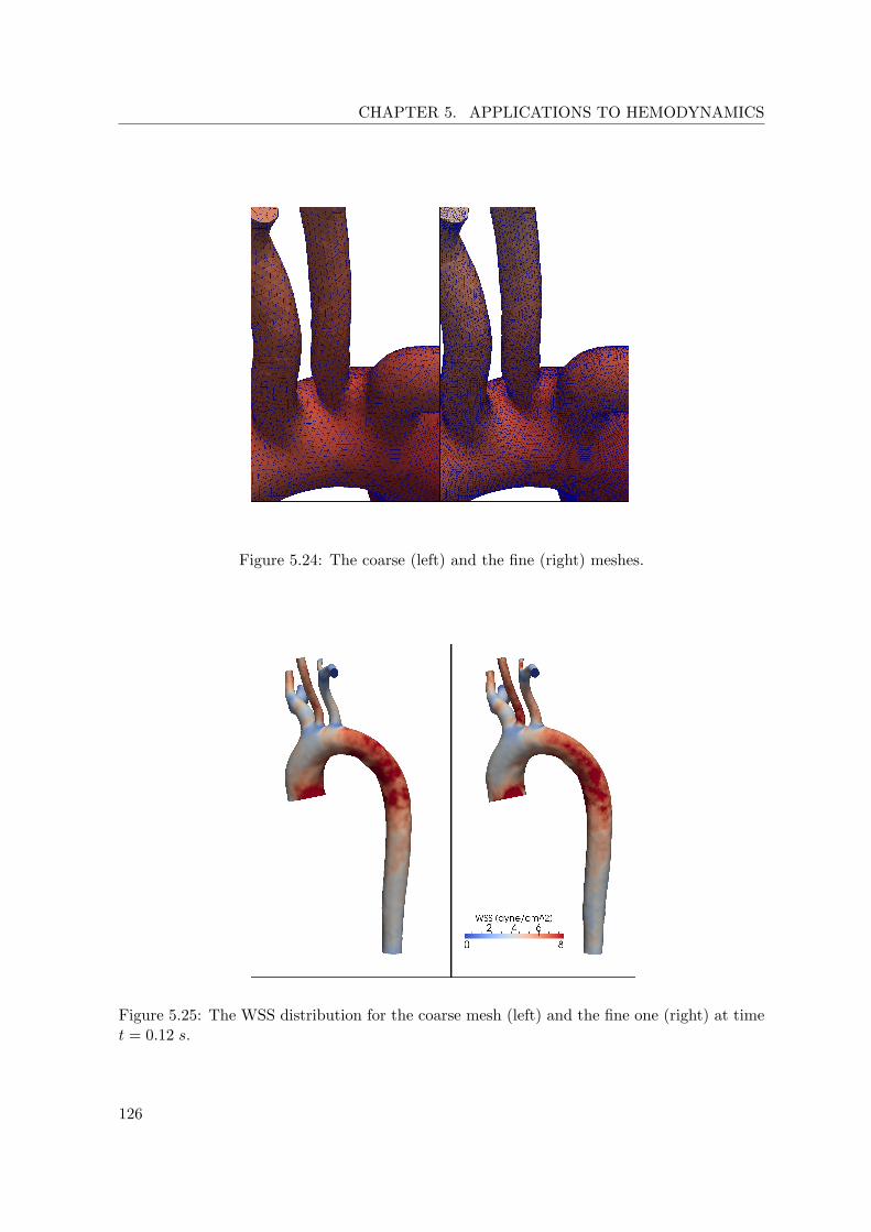
CHAPTER 5. APPLICATIONS TO HEMODYNAMICS
Figure 5.24: The coarse (left) and the fine (right) meshes.
Figure 5.25: The WSS distribution for the coarse mesh (left) and the fine one (right) at timet = 0.12 s.
126
5.4. BLOOD FLOW IN THE AORTA
in Newtonian fluids it is
τ = σfnf − (σfnf · nf )nf = µf (∇xu + ∇xuT )nf − µf[(∇xu + ∇xuT ) · nf ] · nfnf(5.4.4)
where µf is the dynamic viscosity. This equation corresponds to
τ = µf [(∇xu +∇xuT )− (∇xu +∇xuT ) : (nf ⊗ nf )]nf .
If u = (u1, u2, u3)T , writing the last equation in Einstein notations we obtain
τj = µf [(∂iuj + ∂jui)− (∂kul + ∂luk)(nknl)δij ]ni.
Fixing a point on the fluid–structure interface we can write all the quantities with respectto the associated local frame of reference (t1, t2,n), where t1 and t2 are orthonormal vectorson the tangent plane and n is the normal vector. We denote the local coordinate systemassociated with this frame (h1, h2, h3). The previous expression reads
τ = µf
(∂h2uh3 + ∂h3uh2)(∂h1uh3 + ∂h3uh1)
0
,
where now uh = (uh1 , uh2 , uh3)T denotes the velocity field written with respect to the localcoodinate system. We notice here that if the fluid wall is fixed every tangential derivative iszero, ∂h1uh3 = 0, ∂h2uh3 = 0. This leads to a straightforward relation between the magnitudeof the wall shear stress and of the vorticity vector ω = ∇× u. In fact we have that
ω =
∂h2uh3 − ∂h3uh2
∂h3uh1 − ∂h1uh3
∂h1uh2 − ∂h2uh1
=
−∂h3uh2
∂h3uh1
0
and thus µf‖ω‖2 = ‖τ‖2.
When the wall is moving this relation is no longer valid. We compute thus in the compliantcase the WSS from relation (5.4.4). However most of the time we do not observe a significantdifference when computing the WSS magnitude through the vorticity vector even in thecompliant walls case. This is perhaps due to the fact that the velocity gradient due tothe boundary layer (the normal derivatives of the tangential velocity) dominates the othercomponents of the velocity gradient. We refer to [WMZ06] for details and discussions aboutshear stress and vorticity relations.
As an example Figure 5.26 shows the wall shear stress (WSS) magnitude in the compliantand rigid walls simulations right after the systole of the second heartbeat. The period ofone heartbeat is T = 0.8 s, so that t = 1 s corresponds approximately to the systolic peak.The WSS distribution is similar at systole with compliant and rigid walls, although it isslightly larger in the latter case. Then at t = 1.1 s and t = 1.2 s the WSS magnitude islarger in the rigid walls case. In particular the WSS in the rigid walls simulation seems to beoverestimated. The systolic WSS are in the physiological range, especially in the compliantcase, if compared with measurements obtained in [BLS10] for the control patients. We do notobserve remarkable differences between the two FSI simulations corresponding to differentinlet boundary conditions.
127
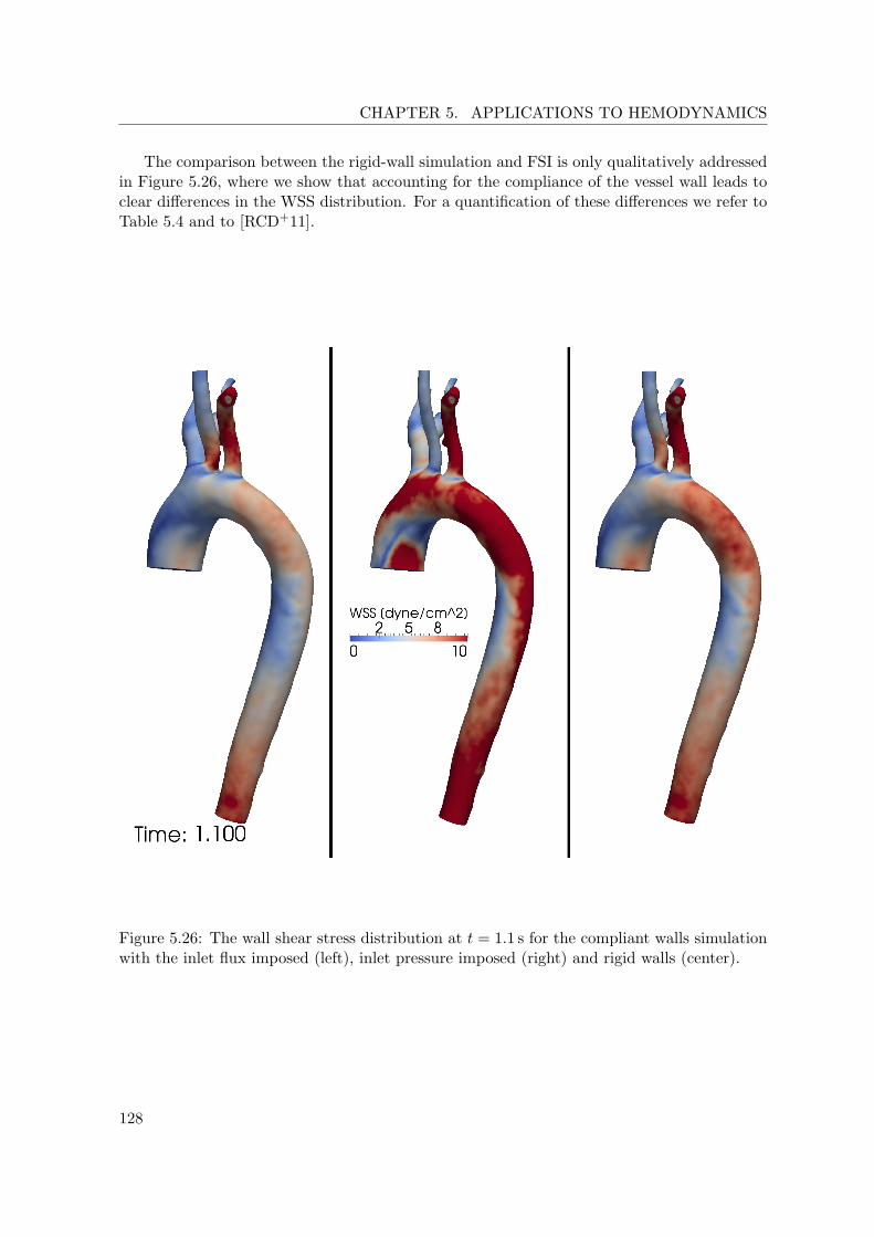
CHAPTER 5. APPLICATIONS TO HEMODYNAMICS
The comparison between the rigid-wall simulation and FSI is only qualitatively addressedin Figure 5.26, where we show that accounting for the compliance of the vessel wall leads toclear differences in the WSS distribution. For a quantification of these differences we refer toTable 5.4 and to [RCD+11].
Figure 5.26: The wall shear stress distribution at t = 1.1 s for the compliant walls simulationwith the inlet flux imposed (left), inlet pressure imposed (right) and rigid walls (center).
128
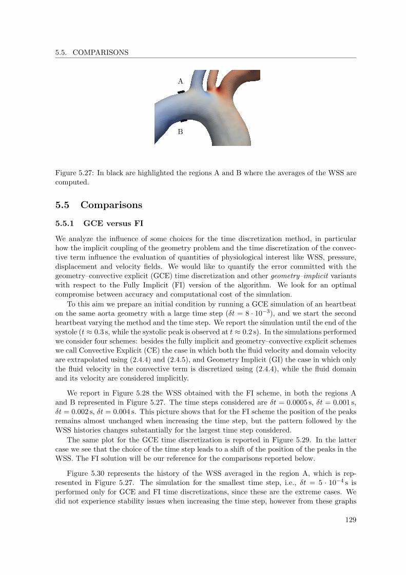
5.5. COMPARISONS
B
A
Figure 5.27: In black are highlighted the regions A and B where the averages of the WSS arecomputed.
5.5 Comparisons
5.5.1 GCE versus FI
We analyze the influence of some choices for the time discretization method, in particularhow the implicit coupling of the geometry problem and the time discretization of the convec-tive term influence the evaluation of quantities of physiological interest like WSS, pressure,displacement and velocity fields. We would like to quantify the error committed with thegeometry–convective explicit (GCE) time discretization and other geometry–implicit variantswith respect to the Fully Implicit (FI) version of the algorithm. We look for an optimalcompromise between accuracy and computational cost of the simulation.
To this aim we prepare an initial condition by running a GCE simulation of an heartbeaton the same aorta geometry with a large time step (δt = 8 · 10−3), and we start the secondheartbeat varying the method and the time step. We report the simulation until the end of thesystole (t ≈ 0.3 s, while the systolic peak is observed at t ≈ 0.2 s). In the simulations performedwe consider four schemes: besides the fully implicit and geometry–convective explicit schemeswe call Convective Explicit (CE) the case in which both the fluid velocity and domain velocityare extrapolated using (2.4.4) and (2.4.5), and Geometry Implicit (GI) the case in which onlythe fluid velocity in the convective term is discretized using (2.4.4), while the fluid domainand its velocity are considered implicitly.
We report in Figure 5.28 the WSS obtained with the FI scheme, in both the regions Aand B represented in Figure 5.27. The time steps considered are δt = 0.0005 s, δt = 0.001 s,δt = 0.002 s, δt = 0.004 s. This picture shows that for the FI scheme the position of the peaksremains almost unchanged when increasing the time step, but the pattern followed by theWSS histories changes substantially for the largest time step considered.
The same plot for the GCE time discretization is reported in Figure 5.29. In the lattercase we see that the choice of the time step leads to a shift of the position of the peaks in theWSS. The FI solution will be our reference for the comparisons reported below.
Figure 5.30 represents the history of the WSS averaged in the region A, which is rep-resented in Figure 5.27. The simulation for the smallest time step, i.e., δt = 5 · 10−4 s isperformed only for GCE and FI time discretizations, since these are the extreme cases. Wedid not experience stability issues when increasing the time step, however from these graphs
129
CHAPTER 5. APPLICATIONS TO HEMODYNAMICS
it is clear that the largest time step fails in predicting the correct value for the averaged WSS,even in the FI case.
Furthermore these graphics show that, for a time step lower then δt = 10−3, in thesimulation of the aortic arch a GCE time discretization provides an approximation of the WSSwhich can be satisfactory, since it qualitatively follows the one obtained with the geometry–implicit variants.
Another interesting result is the difference between the fully implicit simulation and theGI and CE ones. This suggests that considering implicitly the part of the convective termnonlinear in u (2.4.2) brings non negligible changes. On the other hand from the similaritybetween CE and GI we conclude that treating implicitly the nonlinearity in w (2.4.3) in theconvective term does not influence much the WSS in the location considered.
Since the number of Newton iterations in all the geometry implicit variants does not varysubstantially we can conclude that among those the most performant and reliable method isthe FI one. Concerning the GCE time discretization, it is considerably faster than all theother methods for a fixed time step and due to the dissipative behavior it shows to be stablealso for large time steps, thus it can provide a fast, not always reliable, prediction of thehemodynamic, or a periodic initial condition for the other methods (as done for the currentsimulations).
In Figure 5.31 the same comparisons are performed on a different location (location B inFigure 5.27). The WSS is well approximated by the GCE especially before the systolic peakand for small time steps (below 1 ms), while it smooths most of the oscillations for largertime steps. As in the previous case the difference when considering the nonlinear term in uis important, while considering explicitly the domain velocity w in the convective term doesnot lead to substantial changes.
We report in Figure 5.34 and Figure 5.32 also the pressure and displacement in the regionA obtained with the different time steps and discretization schemes. The same comparisonfor region B is shown in Figures 5.35 and 5.33. We notice from these pictures that the GCEtime discretization, though being stable for all the time steps tested, fails in reproducing thetime history of pressure and displacement of the FI for large time steps. The time step shouldthus be tuned according to the output of interest and to the precision requested.
Eventually we report in Figure 5.36 a comparison of the mean velocities and pressurescomputed with the various schemes for a fixed timestep of δt = 10−3. The quantities rep-resented are the averages on a section of the lumen in the descending aortic arch. We seefrom this plot that the difference between pressure and flux on a section of the lumen is smallcompared to the difference observed on the regions A and B of the arterial wall (Figure 5.27).
A picture of the reference solution (the FI simulation with time step δt = 0.0005 s) isrepresented in Figure 5.37 together with the WSS distribution at the end-systole. The de-creasing of the inlet flux originates vortices in the ascending aorta, while the streamlines showthe presence of secondary flows in the descending part of the aortic arch. This behavior istypical for blood flow in a curved vessel (see e.g. Doorly and Sherwin [FQV09, Ch. 5.3]). Thesimulations were run on the Cray XT4 cluster in HECToR, using 64 MPI processes (4 pernode).
130
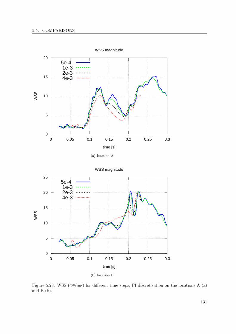
5.5. COMPARISONS
0
5
10
15
20
0 0.05 0.1 0.15 0.2 0.25 0.3
WS
S
time [s]
WSS magnitude
5e-4 1e-32e-34e-3
(a) location A
0
5
10
15
20
25
0 0.05 0.1 0.15 0.2 0.25 0.3
WS
S
time [s]
WSS magnitude
5e-4 1e-32e-34e-3
(b) location B
Figure 5.28: WSS (dyn/cm2) for different time steps, FI discretization on the locations A (a)and B (b).
131

CHAPTER 5. APPLICATIONS TO HEMODYNAMICS
0
5
10
15
20
0 0.05 0.1 0.15 0.2 0.25 0.3
WS
S
time [s]
WSS magnitude
5e-4 1e-32e-34e-3
(a) location A
0
5
10
15
20
25
0 0.05 0.1 0.15 0.2 0.25 0.3
WS
S
time [s]
WSS magnitude
5e-4 1e-32e-34e-3
(b) location B
Figure 5.29: WSS (dyn/cm2) for different time steps, GCE discretization on the locations A(a) and B (b).
132

5.5. COMPARISONS
0
5
10
15
20
0 0.05 0.1 0.15 0.2 0.25 0.3
WS
S
time [s]
WSS magnitude
FI GCE
(a) δt = 5 · 10−4 s
0
5
10
15
20
0 0.05 0.1 0.15 0.2 0.25 0.3
WS
S
time [s]
WSS magnitude
FI GCE
GICE
(b) δt = 10−3 s
133

CHAPTER 5. APPLICATIONS TO HEMODYNAMICS
0
5
10
15
20
0 0.05 0.1 0.15 0.2 0.25 0.3
WS
S
time [s]
WSS magnitude
FI GCE
GICE
(c) δt = 2 · 10−3 s
0
5
10
15
20
0 0.05 0.1 0.15 0.2 0.25 0.3
WS
S
time [s]
WSS magnitude
FI GCE
GICE
(d) δt = 4 · 10−3 s
Figure 5.30: Time history of the WSS magnitude (in dyn/cm2) averaged on the location A ofFigure 5.27.134
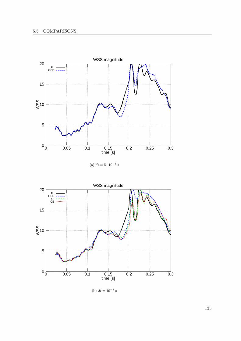
5.5. COMPARISONS
0
5
10
15
20
0 0.05 0.1 0.15 0.2 0.25 0.3
WS
S
time [s]
WSS magnitude
FI GCE
(a) δt = 5 · 10−4 s
0
5
10
15
20
0 0.05 0.1 0.15 0.2 0.25 0.3
WS
S
time [s]
WSS magnitude
FI GCE
GICE
(b) δt = 10−3 s
135

CHAPTER 5. APPLICATIONS TO HEMODYNAMICS
0
5
10
15
20
0 0.05 0.1 0.15 0.2 0.25 0.3
WS
S
time [s]
WSS magnitude
FI GCE
GICE
(c) δt = 2 · 10−3 s
0
5
10
15
20
0 0.05 0.1 0.15 0.2 0.25 0.3
WS
S
time [s]
WSS magnitude
FI GCE
GICE
(d) δt = 4 · 10−3 s
Figure 5.31: Time history of the WSS magnitude (in dyn/cm2) averaged on the location B ofFigure 5.27.136
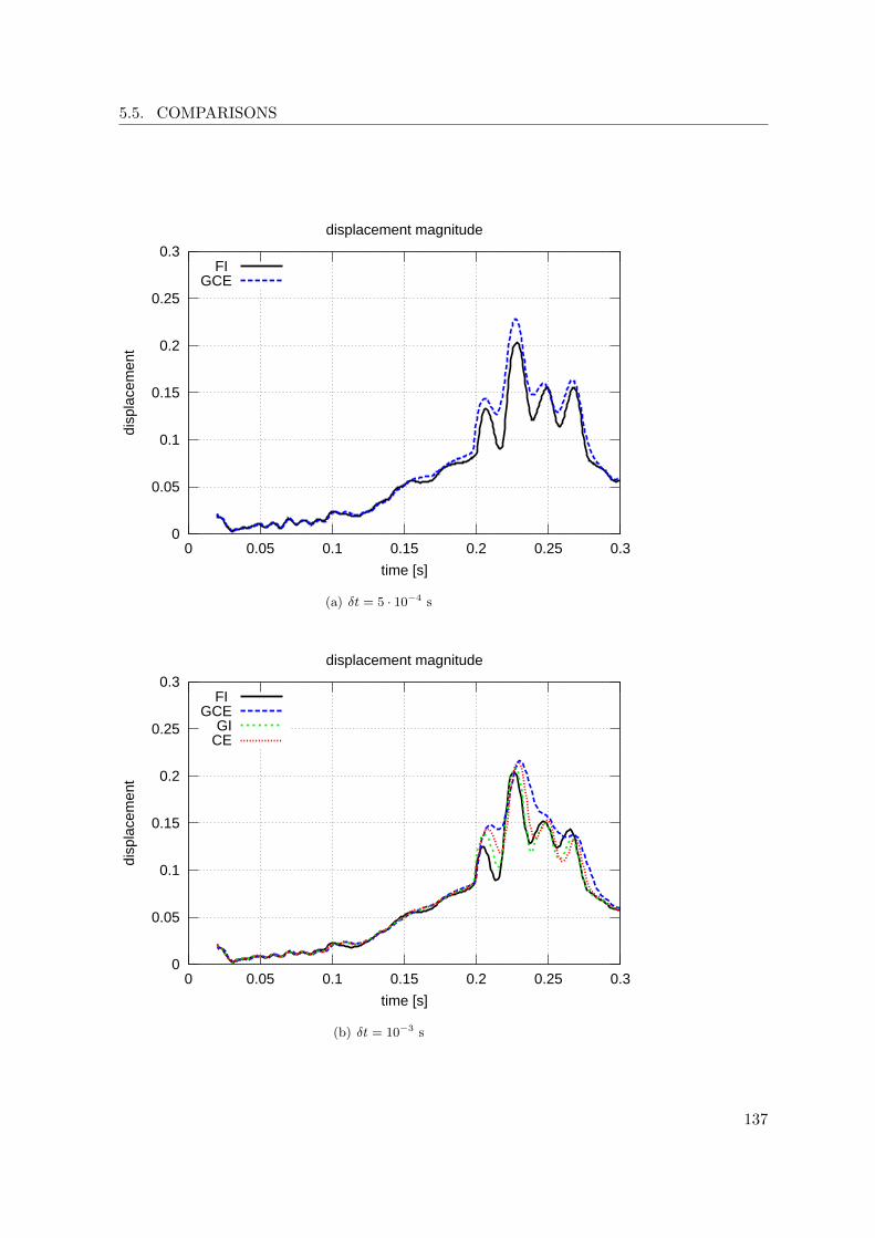
5.5. COMPARISONS
0
0.05
0.1
0.15
0.2
0.25
0.3
0 0.05 0.1 0.15 0.2 0.25 0.3
disp
lace
men
t
time [s]
displacement magnitude
FI GCE
(a) δt = 5 · 10−4 s
0
0.05
0.1
0.15
0.2
0.25
0.3
0 0.05 0.1 0.15 0.2 0.25 0.3
disp
lace
men
t
time [s]
displacement magnitude
FI GCE
GICE
(b) δt = 10−3 s
137

CHAPTER 5. APPLICATIONS TO HEMODYNAMICS
0
0.05
0.1
0.15
0.2
0.25
0.3
0 0.05 0.1 0.15 0.2 0.25 0.3
disp
lace
men
t
time [s]
displacement magnitude
FI GCE
GICE
(c) δt = 2 · 10−3 s
0
0.05
0.1
0.15
0.2
0.25
0.3
0 0.05 0.1 0.15 0.2 0.25 0.3
disp
lace
men
t
time [s]
displacement magnitude
FI GCE
GICE
(d) δt = 4 · 10−3 s
Figure 5.32: Time history of the displacement magnitude (in cm) averaged on the location Aof Figure 5.27.
138

5.5. COMPARISONS
0
0.05
0.1
0.15
0.2
0.25
0.3
0 0.05 0.1 0.15 0.2 0.25 0.3
disp
lace
men
t
time [s]
displacement magnitude
FI GCE
(a) δt = 5 · 10−4 s
0
0.05
0.1
0.15
0.2
0.25
0.3
0 0.05 0.1 0.15 0.2 0.25 0.3
disp
lace
men
t
time [s]
displacement magnitude
FI GCE
GICE
(b) δt = 10−3 s
139

CHAPTER 5. APPLICATIONS TO HEMODYNAMICS
0
0.05
0.1
0.15
0.2
0.25
0.3
0 0.05 0.1 0.15 0.2 0.25 0.3
disp
lace
men
t
time [s]
displacement magnitude
FI GCE
GICE
(c) δt = 2 · 10−3 s
0
0.05
0.1
0.15
0.2
0.25
0.3
0 0.05 0.1 0.15 0.2 0.25 0.3
disp
lace
men
t
time [s]
displacement magnitude
FI GCE
GICE
(d) δt = 4 · 10−3 s
Figure 5.33: Time history of the displacement magnitude (in cm) averaged on the location Bof Figure 5.27.
140

5.5. COMPARISONS
-10
0
10
20
30
40
50
0 0.05 0.1 0.15 0.2 0.25 0.3
pres
sure
time [s]
pressure magnitude
FI GCE
(a) δt = 5 · 10−4 s
-10
0
10
20
30
40
50
0 0.05 0.1 0.15 0.2 0.25 0.3
pres
sure
time [s]
pressure magnitude
FI GCE
GICE
(b) δt = 10−3 s
141

CHAPTER 5. APPLICATIONS TO HEMODYNAMICS
-10
0
10
20
30
40
50
0 0.05 0.1 0.15 0.2 0.25 0.3
pres
sure
time [s]
pressure magnitude
FI GCE
GICE
(c) δt = 2 · 10−3 s
-10
0
10
20
30
40
50
0 0.05 0.1 0.15 0.2 0.25 0.3
pres
sure
time [s]
pressure magnitude
FI GCE
GICE
(d) δt = 4 · 10−3 s
Figure 5.34: Time history of the pressure (in mmHg) averaged on the location A of Figure 5.27.
142
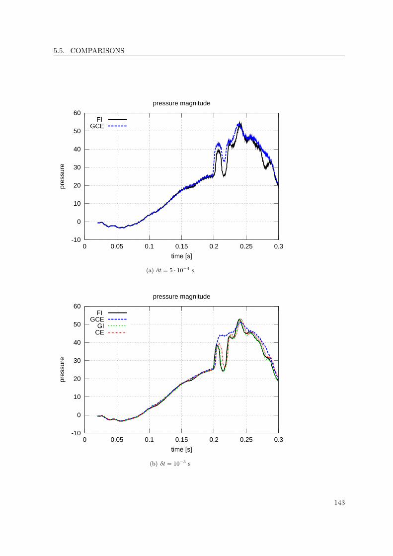
5.5. COMPARISONS
-10
0
10
20
30
40
50
60
0 0.05 0.1 0.15 0.2 0.25 0.3
pres
sure
time [s]
pressure magnitude
FI GCE
(a) δt = 5 · 10−4 s
-10
0
10
20
30
40
50
60
0 0.05 0.1 0.15 0.2 0.25 0.3
pres
sure
time [s]
pressure magnitude
FI GCE
GICE
(b) δt = 10−3 s
143

CHAPTER 5. APPLICATIONS TO HEMODYNAMICS
-10
0
10
20
30
40
50
60
0 0.05 0.1 0.15 0.2 0.25 0.3
pres
sure
time [s]
pressure magnitude
FI GCE
GICE
(c) δt = 2 · 10−3 s
-10
0
10
20
30
40
50
60
0 0.05 0.1 0.15 0.2 0.25 0.3
pres
sure
time [s]
pressure magnitude
FI GCE
GICE
(d) δt = 4 · 10−3 s
Figure 5.35: Time history of the pressure (in mmHg) averaged on the location B of Figure 5.27.
144

5.5. COMPARISONS
-5
0
5
10
15
20
25
30
0 0.05 0.1 0.15 0.2 0.25 0.3 0.35
pres
sure
time [s]
pressure magnitude
FI GCE
GICE
(a) mean pressure
0
10
20
30
40
50
60
70
80
0 0.05 0.1 0.15 0.2 0.25 0.3 0.35
velo
city
time [s]
velocity magnitude
FI GCE
GICE
(b) mean velocity
Figure 5.36: Values of the mean pressure (in mmHg) and mean velocity (in cm/s) on a sectionof the descending aortic arch, for the different time discretizations and with a fixed time stepof δt = 10−3. 145

CHAPTER 5. APPLICATIONS TO HEMODYNAMICS
Figure 5.37: Aorta simulation. Streamlines and WSS at the end of the systolic phase in thesecond heartbeat.
146

5.5. COMPARISONS
5.5.2 Exact versus Inexact Newton Method
In the cases where the geometry is handled implicitly a Newton method is employed. Thenumber of Newton iterations as expected varies depending on the time step chosen and onthe phase of the heartbeat considered. In particular in proximity of the systolic peak, dueto the large displacements and velocities, the nonlinearities due to both convective term andgeometry become important, and the number of Newton iterations increases. Due to the factthat the convergence of Newton is not assured when the initial guess is far from the solution,for large time steps in some cases we experienced convergence problems in proximity of thesystolic peak. Since the first order methods have usually a larger convergence ball then theNewton method (see e.g. [ESW05, Ch. 7]), a fixed point or inexact Newton method couldbe employed to reach a closer initial state for the Newton method27. Here we consider onlyfirst order extrapolations and discretizations. Testing more accurate time discretizations iscurrently under investigation.
We investigate in the simulation of the GI solution the effect of taking into account theshape derivatives in the Jacobian of the FSI problem. The number of Newton iterationsperformed during systole (i.e., from t = 0.16 s to t = 2.4 s) in both cases is reported inFigure 5.38 for a time step of δt = 0.004 s, the relative tolerance (see Section 3.1) is setto εr = 10−4. Using the exact Jacobian matrix in this case not only improves the solutionin terms of nonlinear iterations: also the performances in terms of CPU time are better.We report the computational cost per time level in Figure 5.38. We recall that if a smartimplementation of the shape derivatives block assembly is exploited (see Section §3.4), thenincreasing the number of processors the overhead becomes negligible with respect to e.g. thematrix-vector multiplications required for the GMRES solution. At the first time iterationconsidered, both exact and inexact Newton perform three iterations (Figure 5.38 on the left),however the time spent in both cases (Figure 5.38 on the right) is almost the same. Inour algorithm the main extra computational cost for the construction of the Jacobian JFIwith respect to the matrix of the system (computed to evaluate the residual) is in the shapederivatives block computation. This block assembly performed once per Newton step has acomputational cost of about 0.8 s for the simulation here presented, which is negligible withrespect to the total time (≈ 1% of the time per Newton iteration) and since it does not requireinter processors communication (like all the matrix assembling steps) it is almost perfectlyscalable.
We remark that for both the inexact and exact Newton schemes the preconditioner usedis PAS−DN (4.2.20), thus the shape derivatives block is not neglected in the preconditioner.Using this preconditioner the number of iterations and the time needed for the solution ofthe linear Jacobian system is not remarkably affected by the presence of the shape derivativesblock.
Remark 5.5.1. These results are somehow in disagreement with what is stated in Bazilevset al. [BGH+09], where an inexact Newton is employed to solve the geometrical nonlinearity,neglecting the shape derivative terms, for the simulation a Ventricular Assisted Device (VAD)
27Many efficient ways to find an accurate initial state for Newton have been studied in literature. For instancein [BC10b] a nonlinear coarse problem is solved at each time iteration just to initialize the nonlinear solver(leading to the two levels Newton method), in [GK10, TDV07] efficient extrapolation techniques based on PODare used in order to accelerate the convergence of a linear or nonlinear solver by improving the initial guess.In [KGF+09, KW09] a vector extrapolation technique allows to move gradually from fixed point iterations toNewton.
147

CHAPTER 5. APPLICATIONS TO HEMODYNAMICS
implanted in a thoracic aorta. There the authors do not find great advantages in consideringthe shape derivatives terms in the Jacobian matrix. We conclude that the debate is still openand so far there is no method which behaves better than the others in all the situations.
Remark 5.5.2. The Newton scheme used is not completely exact, because the fluxes areprescribed as integrals on moving boundaries (the vessel terminations are not clamped), andthe shape derivatives of these terms (cf. Section §3.4.2) are not taken into account in ourJacobian.
2
3
4
5
6
7
8
5 10 15 20
New
ton
itera
tions
Time iteration
Newton iterations
NQN
(a)
200
250
300
350
400
450
0 5 10 15 20 25
time
(s)
CPU time per time iteration
QN
Time iteration
N
(b)
Figure 5.38: Aorta simulation: (a) number of Newton iterations and (b) CPU time per timestep. Exact Newton (N) is compared versus inexact Newton (QN) for an interval during thesystolic peak (from t = 0.16 s to t = 0.24 s) for a GI simulation with time step δt = 0.004 s
148
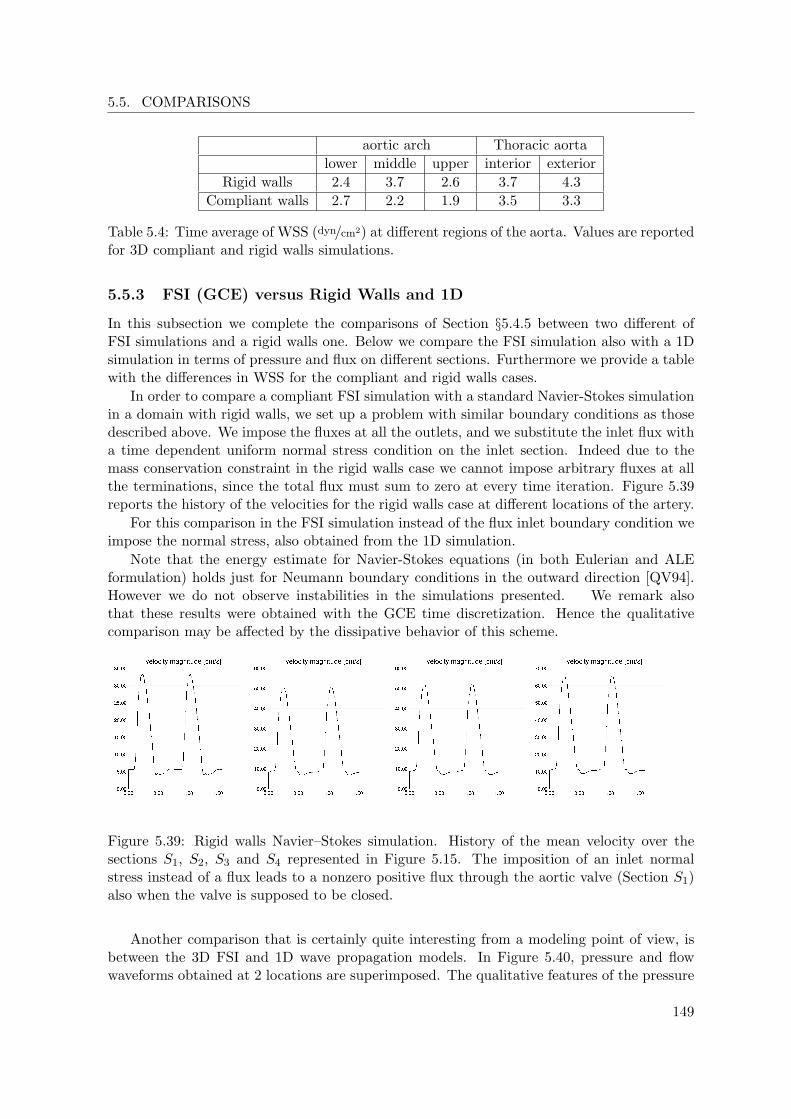
5.5. COMPARISONS
aortic arch Thoracic aortalower middle upper interior exterior
Rigid walls 2.4 3.7 2.6 3.7 4.3Compliant walls 2.7 2.2 1.9 3.5 3.3
Table 5.4: Time average of WSS (dyn/cm2) at different regions of the aorta. Values are reportedfor 3D compliant and rigid walls simulations.
5.5.3 FSI (GCE) versus Rigid Walls and 1D
In this subsection we complete the comparisons of Section §5.4.5 between two different ofFSI simulations and a rigid walls one. Below we compare the FSI simulation also with a 1Dsimulation in terms of pressure and flux on different sections. Furthermore we provide a tablewith the differences in WSS for the compliant and rigid walls cases.
In order to compare a compliant FSI simulation with a standard Navier-Stokes simulationin a domain with rigid walls, we set up a problem with similar boundary conditions as thosedescribed above. We impose the fluxes at all the outlets, and we substitute the inlet flux witha time dependent uniform normal stress condition on the inlet section. Indeed due to themass conservation constraint in the rigid walls case we cannot impose arbitrary fluxes at allthe terminations, since the total flux must sum to zero at every time iteration. Figure 5.39reports the history of the velocities for the rigid walls case at different locations of the artery.
For this comparison in the FSI simulation instead of the flux inlet boundary condition weimpose the normal stress, also obtained from the 1D simulation.
Note that the energy estimate for Navier-Stokes equations (in both Eulerian and ALEformulation) holds just for Neumann boundary conditions in the outward direction [QV94].However we do not observe instabilities in the simulations presented. We remark alsothat these results were obtained with the GCE time discretization. Hence the qualitativecomparison may be affected by the dissipative behavior of this scheme.
Figure 5.39: Rigid walls Navier–Stokes simulation. History of the mean velocity over thesections S1, S2, S3 and S4 represented in Figure 5.15. The imposition of an inlet normalstress instead of a flux leads to a nonzero positive flux through the aortic valve (Section S1)also when the valve is supposed to be closed.
Another comparison that is certainly quite interesting from a modeling point of view, isbetween the 3D FSI and 1D wave propagation models. In Figure 5.40, pressure and flowwaveforms obtained at 2 locations are superimposed. The qualitative features of the pressure
149

CHAPTER 5. APPLICATIONS TO HEMODYNAMICS
waveforms are in good agreement. The amplitude of the flow waveforms is slightly different,mainly in systole, at both aortic cross and thoracic aorta.
Figure 5.40: Pressure (top) and flow (bottom) waveforms computed by the FSI simulation(continuous line) and the 1D model (dashed line). Locations are at the aortic arch (left) andthoracic aorta (right). Fluxes are imposed at the inlet and all the outlets.
150

Scalability and ParallelPerformances
6.1 Introduction
In this chapter we investigate the parallel performance of the FSI solver in LifeV. In theprevious chapter we already reported some results concerning CPU time and computationalcost. Here we complete these informations by studying the behavior of the solver when varyingthe number of MPI processes and/or the problem size.
To organize the discussion we report first a definition of scalable algorithm. Indeed de-pending on the field the concepts of weak and strong scalability may have slightly differentmeanings. We report then weak and strong scalability results for some of the preconditionersdescribed in Section §4.3 on benchmark and physiological geometries.
6.2 Scalability and Results
In parallel computing a very important concept is the one of scalability, which is a measureof the capability of an algorithm to perform when increasing workload and/or the number ofparallel processes.
Although the term scalability is widely used throughout literature in several applicationfields, many different interpretations and operational definitions coexist. This issue is ad-dressed e.g. in Keyes [Key98] where a general definition is given which makes abstractionfrom the specific application considered. There the definition of scalability requires a perfor-mance metric which is a function of several parameters πi. The performance function chosenstrongly influences the type of scalability considered, which is usually reached for a boundedregion in the parameters space.
The performance function that we consider is the parallel efficiency. It is usually measuredin floating point operations per seconds when the hardware scalability is investigated. In ourapplication we define the parallel efficiency of an operation as the inverse of the time spentfor such operation. We express the performance η in terms of two parameters: the workloadand the processors number. The workload in our case is the number of degrees of freedom ofthe problem. Two types of scalability, listed below, are usually considered.
• Strong scalability: in a strongly scalable algorithm doubling the number of processors(and keeping fixed the other parameters) the efficiency doubles as well. In practicalcases this type of scalability is never reached because of the hardware limitations: theoverall time is the sum of the time spent for the computations and the time spentfor the communications between the processors. While for the former operations the
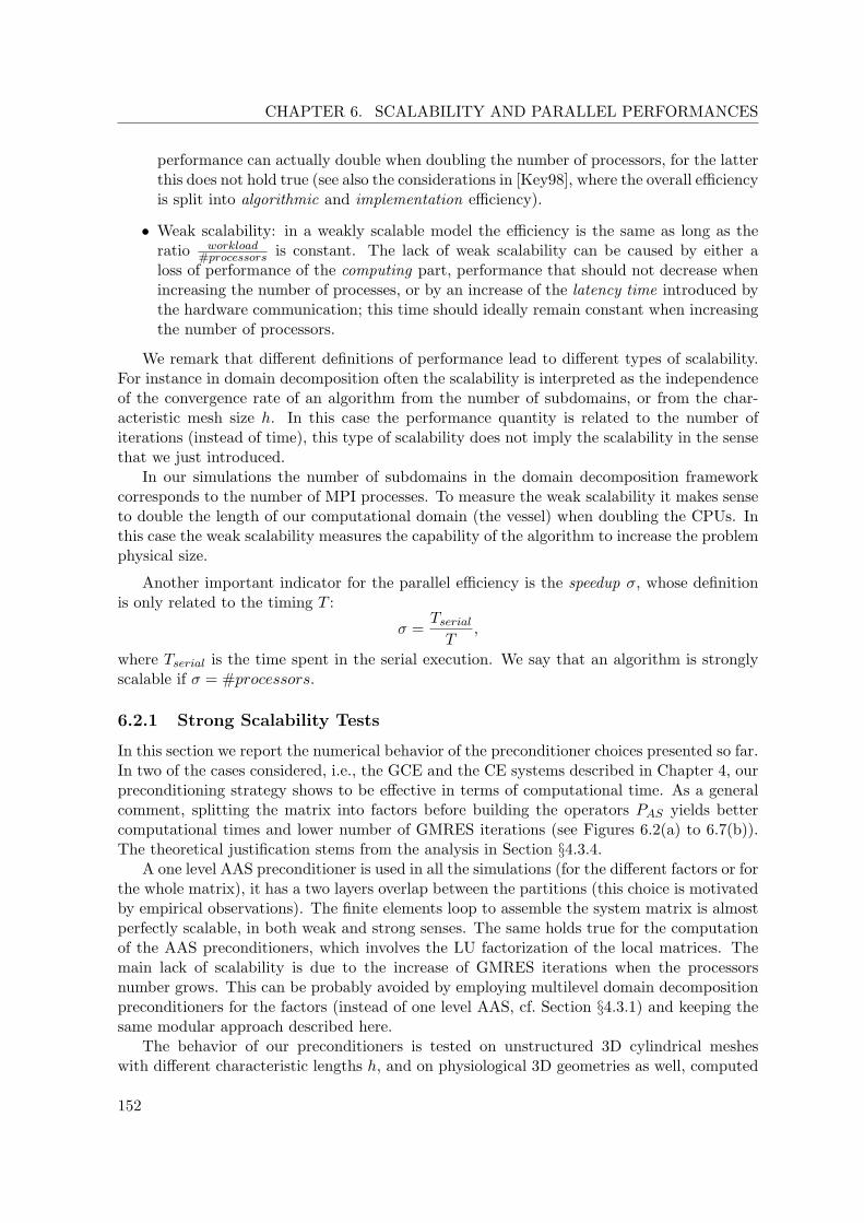
CHAPTER 6. SCALABILITY AND PARALLEL PERFORMANCES
performance can actually double when doubling the number of processors, for the latterthis does not hold true (see also the considerations in [Key98], where the overall efficiencyis split into algorithmic and implementation efficiency).
• Weak scalability: in a weakly scalable model the efficiency is the same as long as theratio workload
#processors is constant. The lack of weak scalability can be caused by either aloss of performance of the computing part, performance that should not decrease whenincreasing the number of processes, or by an increase of the latency time introduced bythe hardware communication; this time should ideally remain constant when increasingthe number of processors.
We remark that different definitions of performance lead to different types of scalability.For instance in domain decomposition often the scalability is interpreted as the independenceof the convergence rate of an algorithm from the number of subdomains, or from the char-acteristic mesh size h. In this case the performance quantity is related to the number ofiterations (instead of time), this type of scalability does not imply the scalability in the sensethat we just introduced.
In our simulations the number of subdomains in the domain decomposition frameworkcorresponds to the number of MPI processes. To measure the weak scalability it makes senseto double the length of our computational domain (the vessel) when doubling the CPUs. Inthis case the weak scalability measures the capability of the algorithm to increase the problemphysical size.
Another important indicator for the parallel efficiency is the speedup σ, whose definitionis only related to the timing T :
σ =TserialT
,
where Tserial is the time spent in the serial execution. We say that an algorithm is stronglyscalable if σ = #processors.
6.2.1 Strong Scalability Tests
In this section we report the numerical behavior of the preconditioner choices presented so far.In two of the cases considered, i.e., the GCE and the CE systems described in Chapter 4, ourpreconditioning strategy shows to be effective in terms of computational time. As a generalcomment, splitting the matrix into factors before building the operators PAS yields bettercomputational times and lower number of GMRES iterations (see Figures 6.2(a) to 6.7(b)).The theoretical justification stems from the analysis in Section §4.3.4.
A one level AAS preconditioner is used in all the simulations (for the different factors or forthe whole matrix), it has a two layers overlap between the partitions (this choice is motivatedby empirical observations). The finite elements loop to assemble the system matrix is almostperfectly scalable, in both weak and strong senses. The same holds true for the computationof the AAS preconditioners, which involves the LU factorization of the local matrices. Themain lack of scalability is due to the increase of GMRES iterations when the processorsnumber grows. This can be probably avoided by employing multilevel domain decompositionpreconditioners for the factors (instead of one level AAS, cf. Section §4.3.1) and keeping thesame modular approach described here.
The behavior of our preconditioners is tested on unstructured 3D cylindrical mesheswith different characteristic lengths h, and on physiological 3D geometries as well, computed
152

6.2. SCALABILITY AND RESULTS
Figure 6.1: The cylindrical geometry used partitioned into 4 subdomains. One processorholds one solid and one fluid subdomain. However, in general, the two are not matchingon the interface (despite the impression given by the picture) and the partitioning is doneindependently for the two meshes.
through segmentation of medical images (e.g. CT scans or MRI). The finite elements chosenare P1−P1 tetrahedra for the fluid, stabilized using the interior penalty technique describedin [PB05], cf. Section §2.7.1, and P1 tetrahedra for the structure.
The tests reported in this section, unless otherwise specified, were performed on the clusterCallisto at EPFL.
Strong Scalability for GCE
A benchmark geometry, similar to the one proposed in [GV03] (and used e.g. in [DDFQ06,KGF+09, FM05]) consists of a straight cylinder of length 10 cm and with radius 0.5 cm rep-resenting the fluid domain, surrounded by a structure of constant thickness 0.1 cm (see Fig-ure 6.1). The inlet boundary condition on the fluid domain is a pressure step function, takingthe constant value pin = 1.33 · 104 dyn/cm2 for t ≤ 0.003 s. The boundary conditions for theoutlet and for the external structure are of Neumann homogeneous type. The time step usedis δt = 10−3 s while the parameters characterizing the model are fluid viscosity µf = 0.03 P,the Young modulus ε = 3 · 106 dyn/cm2, the Poisson ratio ν = 0.3 and the mass densities offluid and structure ρf = 1.0 g/cm3 and ρs = 1.2 g/cm3. Because of the GCE time discretizationadopted, the problem is linear. The tolerance for the GMRES solver is 10−6. The valuesreported in the following are the average over the first 30 time iterations.
The simulations run on the benchmark geometry show that the modular preconditionersPAS−DN1 and PAS−DN2 (P (1) and P (2) respectively in the figures) are more efficient thanAAS (a classical additive Schwarz preconditioner on the whole matrix) in terms of compu-tational time and GMRES iterations. Furthermore the gap between these preconditioningstrategies increases with the processors number. This result is validated on two differentmeshes composed by a total of 169′267 and 578′594 tetrahedra, corresponding to respectively216′441 and 630′468 degrees of freedom (in Figures 6.2(a) and 6.2(b)), and varying the ratiobetween the mass densities r = ρf
ρs(in Figure 6.3).
We observe that in view of the analysis performed in Section §4.3.4 the mild growth of theGMRES iterations in the modular cases can be explained with a boundedness of the singularvalue σmaxΣ . We recall that the preconditioners PAS−DN1 and PAS−DN2 are split into factors,and each factor contains either the fluid or the structure block. The lack of scalability, dueto the increasing number of GMRES iterations, is related to our choice of using the one levelAAS preconditioner for all the factors in the tests performed. Thanks to Proposition 4.3.1the quality of the preconditioner is influenced mainly by the preconditioners chosen for thedifferent factors. Thus an improvement of the preconditioner can be achieved by improvingthe preconditioners for the subproblems.
153

CHAPTER 6. SCALABILITY AND PARALLEL PERFORMANCES
20406080
100120140160
8 16 32 64
# ite
ratio
ns
number of processors
GMRES iterations
P(2)
P(1)
PAS
6
10
20
30
50
8 16 32 64
solu
tion
time
(s)
number of processors
time per GMRES solution
5
10
20
4070
8 16 32 64
time
(s)
number of processors
preconditioner computation
30
50
100140
8 16 32 64
itera
tion
time
(s)
number of processors
cpu time per time step
(a) Simulations run on the coarser tube mesh.
6080
100120140160180200
16 32 64
# ite
ratio
ns
number of processors
GMRES iterations
P(2)
P(1)
PAS
30406090
130
200300400
16 32 64 16
solu
tion tim
e (
s)
number of processors
time per GMRES solution
16 32 6410
20
4070
150
300
16 32 64tim
e (s
)number of processors
preconditioner computation
100
200300400600900
16 32 64
itera
tion
time
(s)
number of processors
cpu time per time step
(b) Simulations run on the finer tube mesh.
Figure 6.2: GCE — Strong scalability. P (1) and P (2) correspond to PAS−DN1 and PAS−DN2
respectively.
Other strong scalability results performed on different architectures, with different spacediscretizations, are resumed in Figures 6.4(a), 6.4(b) and 6.4(c). These simulations arerun on a segment of thoracic aorta, and the linear system is preconditioned by PAS−DN1.Figures 6.4(a) to 6.4(c) show the total CPU time per time step, the time to compute thepreconditioner, the time to solve the linear problem and the number of GMRES iterations ateach time step. The number of tetrahedra is 578′594.
Figures 6.4(a) and 6.4(b) refer to the same simulation on the Cray XT4 and on the BlueGene/P, where the finite elements used for the fluid subproblem are the stabilized P1-P1elements. The total number of unknowns in this case is 630′468. With the same numberof processors, the simulation on an XT4 takes about 3.5 times less CPU time than on aBlueGene/P (this is a consequence of the different CPU frequency); in contrast, the scalabilityof the overall simulation is better on the BlueGene/P. Figure 6.4(c) represents the same typeof simulation with inf–sup stable P1Bubble-P1 (mini) finite elements for the fluid problem.On BlueGene/P we notice an improvement of the scalability with 512 processors. The CPUtime is smaller than for P1-P1 since the stencil of the matrix is smaller.
We remark that in these simulations the number of GMRES iterations does not increasewhen the number of processors increases.
Strong Scalability for CE
We run the same simulation as for the GCE on the straight cylinder. The tolerance of thelinear solver is set to 10−6 while the relative tolerance for the Newton method is εr = 10−5.
The preconditioners compared in Figure 6.5(a) are PAS(JCE), PAS−QN (without splittinginto factors) and PAS−GS (two factors splitting) among those listed in Section §4.3.3. Weobserve that the preconditioner PAS−QN is cheaper to compute than PAS(JCE), while it has
154

6.2. SCALABILITY AND RESULTS
20
40
60
80
100
120
140
160
8 16 32 64
# ite
ratio
ns
number of processors
GMRES iterations
P(2), r=100 P(1), r=100PAS, r=100
P(2), r=0.01 P(1), r=0.01PAS, r=0.01
P(2), r=1 P(1), r=1PAS, r=1
6
10
20
30
40
50
8 16 32 64
solu
tion
time
(s)
number of processors
time per GMRES solution
3
5
10
20
40
70
8 16 32 64
time
(s)
number of processors
preconditioner computation
20
30
50
80
150
8 16 32 64
itera
tion
time
(s)
number of processors
cpu time per time step
Figure 6.3: GCE — Comparison on the coarser tube mesh between the results obtained fordifferent values of the ratio r = ρf/ρs.
the same behavior in terms of GMRES iterations. Although PAS−GS is cheaper to computethan the other choices it worsen faster when increasing the number of processors. This canbe due to the growth of the singular value σΣ in the estimate (4.3.10a), when augmentingthe number of processors. Thus PAS−GS seems not to be a choice well suited for a massivelyparallel framework.
155

CHAPTER 6. SCALABILITY AND PARALLEL PERFORMANCES
AS-DN1
(a) stabilized P1P1 finite elements for fluid sub-problem, results on Cray XT4.
AS
AS-DN1
(b) stabilized P1P1 finite elements for fluid sub-problem, results on BlueGene/P.
AS-DN1
(c) P1BubbleP1 finite elements for fluid sub-problem,results on BlueGene/P.
Figure 6.4: GCE time discretization. The dashed line represents the ideal case.
0
50
100
150
200
8 16 32 64
# ite
ratio
ns
number of processors
GMRES iterations
PPAS-QN
PAS
AS-GS
50
60
70
90
110
8 16 32 64
solu
tion
time
(s)
number of processors
time per GMRES solution
610
20
40
80
150
8 16 32 64
time
(s)
number of processors
preconditioner computation
200
280
350
550
8 16 32 64
itera
tion
time
(s)
number of processors
cpu time per time step
(a) coarser tube mesh.
50100150200250300350400
32 64 128
# ite
ratio
ns
number of processors
GMRES iterations
PAS-GS
PAS-QNPAS
200 230
280
350
450
32 64 128
solu
tion
time
(s)
number of processors
time per GMRES solution
10
20
4070
150
300
32 64 128
time
(s)
number of processors
preconditioner computation
600700
900
1200
1600
32 64 128
itera
tion
time
(s)
number of processors
cpu time per time step
(b) finer tube mesh.
Figure 6.5: CE — Strong scalability on a straight cylinder.
Among the preconditioners presented in Figures 6.5(b) and 6.5(a) the most convenient
156
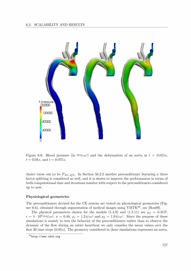
6.2. SCALABILITY AND RESULTS
Figure 6.6: Blood pressure (in dyn/cm2) and the deformation of an aorta at t = 0.015 s,t = 0.03 s, and t = 0.075 s.
choice turns out to be PAS−QN . In Section §6.2.2 another preconditioner featuring a threefactor splitting is considered as well, and it is shown to improve the performances in terms ofboth computational time and iterations number with respect to the preconditioners consideredup to now.
Physiological geometries
The preconditioners devised for the CE system are tested on physiological geometries (Fig-ure 6.6), obtained through segmentation of medical images using VMTK28, see [Bon09].
The physical parameters chosen for the models (1.4.9) and (1.5.11) are µf = 0.35 P,ε = 4 · 106 dyn/cm2, ν = 0.48, ρs = 1.2 g/cm3 and ρf = 1.0 g/cm3. Since the purpose of thesesimulations is mainly to test the behavior of the preconditioners rather than to observe thedynamic of the flow during an entire heartbeat we only consider the mean values over thefirst 30 time steps (0.03 s). The geometry considered in these simulations represents an aorta,
28http://www.vmtk.org
157

CHAPTER 6. SCALABILITY AND PARALLEL PERFORMANCES
20
40
60
80
100
8 16 32 64
# iterations
number of processors
GMRES iterations
PAS-GSPAS-QNPAS
6
10
20
30
8 16 32 64
solu
tion
time
(s)
number of processors
time per GMRES solution
1
5
10
25
8 16 32 64
time
(s)
number of processors
preconditioner computation
50
100
170
300
8 16 32 64
itera
tion
time
(s)
number of processors
cpu time per time step
(a) coarser mesh.
20
40
60
80
100
120
140
32 64 128
# iterations
number of processors
GMRES iterations
PAS-GSPAS-QNPAS
45
60
80
110
150
200
32 64 128
solu
tion
time
(s)
number of processors
time per GMRES solution
58
15255080
150250
32 64 128
time
(s)
number of processors
preconditioner computation
300
450550700900
1200
1700
32 64 128
itera
tion
time
(s)
number of processors
cpu time per time step
(b) finer mesh.
Figure 6.7: CE — Simulations on the aorta on Figure 6.6.
starting from the aortic valve, including the aortic arch and the thoracic aorta. The inletpressure imposed at the aortic valve is taken from physiological measurements correspondingto the beginning of an heartbeat cycle pin ≈ 1.1 · 105 dyn/cm2. The boundary conditionsimposed at the outflows and on the external wall are of Neumann homogeneous type. Sinceno spurious reflection waves are originated in the first 30 time steps (see e.g. [Nob01]), thereis no need to impose absorbing boundary conditions at the outflows. The blood is consideredat rest at the beginning of the simulation. The simulations are performed on two differentmeshes, with respectively 105′810 and 380′690 tetrahedra for a total of 135′000 and 486′749degrees of freedom. We keep the same time step δt = 10−3 s used in the previous simulations.
We can notice that the number of iterations relative to PAS−GS worsens faster than theothers when the number of processors increases (Figures 6.7(a) and 6.7(b)). This phenomenonwas already observed in the previous benchmark tests.
The increase of the global computational time when passing from 32 to 64 processors inthe coarser case is partly due to the relatively small mesh size of the problem addressed andpartly to the communication time affecting both the GMRES solution and the preconditionercomputation.
6.2.2 Weak Scalability Test
We want to set up the same benchmark test with a similar geometry, the same physical param-eters and boundary conditions as in the previous section, but keeping approximately constantthe ratio #dof
#processors . To this aim we build a series of meshes of the tube in Figure 6.8(a)by varying its length. The new meshes are built with the free mesh generator Gmsh29. Thefluid part is generated by building a 2D Delaunay mesh of a circle and extruding it in theaxial direction. The structured solid mesh is generated extruding the lateral surface in thenormal direction. The solid is composed of four layers (see Figure 6.8(a)). We used for thesesimulations the Cray XT5 supercomputer Rosa.
29http://geuz.org/gmsh/
158

6.2. SCALABILITY AND RESULTS
(a) Benchmark mesh (b) Geometries
Figure 6.8: Mesh (a) and geometries (b) used for the weak scalability test. Deformation attime t = 0.01 s.
The different geometries considered have a length varying from 0.5 cm to 16 cm and arerepresented in Figure 6.8(b). The smaller problem is solved using either 12 or 24 MPI pro-cesses, then the number of processors is doubled every time the length of the tube doubles.
The finite elements matrices in this case are considerably worse conditioned than in thecase considered for the strong scalability, the characteristic element size being smaller. The di-mensions for the fluid and the solid meshes considered are resumed in Tables 6.4(a) and 6.4(b)respectively. The larger problem considered, corresponding to the 16 cm pipe in Figure 6.8(b),features 3′517′839 degrees of freedom. The results plotted are the mean values over the first10 time iterations.
(a) fluid meshes.
Length # Elements # Vertices0.5 cm 75’480 14’4871 cm 149’520 27’4052 cm 301’920 53’9974 cm 603’840 106’6778 cm 1’207’680 212’03716 cm 2’415’360 422’757
(b) solid meshes.
Length # Elements # Vertices0.5 cm 27’840 6’3801 cm 55’680 12’1802 cm 111’360 23’7804 cm 222’720 46’9808 cm 445’440 93’38016 cm 890’880 186’180
Table 6.5: Table resuming the characteristics of the meshes used for the weak scalability test,represented in Figure 6.8(b).
Weak Scalability for GCE
In this case the number of linear iterations using the classical AAS preconditioner increasesmuch faster. The new preconditioning strategies proposed show to be more robust. We show
159

CHAPTER 6. SCALABILITY AND PARALLEL PERFORMANCES
50
100
150
200
250
300
24 48 96 192 384 768
# ite
ratio
ns
number of processors
GMRES iterations
P(1)
P(2)
10
20305070
100140180
24 48 96 192 384 768
solu
tion
time
(s)
number of processors
time per GMRES solution
2
4
8
16
32
64
24 48 96 192 384 768
time
(s)
number of processors
preconditioner computation
50
100150200300400
24 48 96 192 384 768
itera
tion
time
(s)
number of processors
cpu time per time step
Figure 6.9: GCE — Weak scalability results for the number of processors ranging from 24 to768.
50100150200250300
2 4 6 12
# ite
ratio
ns
number of processors
GMRES iterations
P(1)
PAS
3040
6080
100
150
2 4 6 12
solu
tion
time
(s)
number of processors
time per GMRES solution
3
8163264
128
2 4 6 12tim
e (s
)
number of processors
preconditioner computation
40
80
160240
400
2 4 6 12
itera
tion
time
(s)
number of processors
cpu time per time step
Figure 6.10: GCE — Strong scaling for the smallest geometry: even with few processors thenumber of iterations increases very fast for PAS , which prevents scalability.
the behavior of the AAS preconditioner compared to PAS−DN1 on the smaller problem for anumber of processors ranging from 2 to 12 in Figure 6.10. We observe that the number ofiterations for the PAS , though it is smaller when considering 2 cores, dramatically increaseswith the number of processors.
We can notice from the weak scalability plot of Figure 6.9 that the GMRES iterationsremain bounded up to 768 processors. The iteration number comparison also shows thatthe performances of PAS−DN1 are slightly better than those of PAS−DN2, however the sametrend is observed in both cases. We notice also the difference of performance between the 24processors case and the 48 processors one: the simulation does not scale in this step. This isprobably due on one hand to the fact that 24 processors fit in two nodes of the cluster, andthe communication between processors in the same node is faster. On the other hand on the0.5 cm tube considered the pressure pulse imposed at the inlet exits the geometry during thefirst time steps, i.e, the characteristics of the simulation are different than in the other cases.We also remark that for the largest simulation the memory of one node is not sufficient whenall the 12 processors are used. For this reason in that case we use only 6 cores per node.The loss of performance when reaching 768 processors is investigated more in detail in thenext paragraph. In conclusion from the “CPU time per time step” plot we see that up to384 processors the code scalability is acceptable. Here we did not represent the scalability ofthe assembling phase for the fluid block, of the solution of the harmonic extension equationand of the HDF5 post processing. However the behavior of these steps is accounted for in the“CPU time per time step” plot in Figure 6.9.
In Figure 6.11 we plot the results of three simulations obtained by varying the sizes ofthe local problems. We call Ni the ratio between the length of the geometry i among thosein Figure 6.8(b) and the length of the shortest pipe (0.5 cm). These simulations have thefollowing specifics:
1. 12 ·Ni processors for the geometry i, using 12 processors per node;
160

6.2. SCALABILITY AND RESULTS
50
100
150
200
250
300
0 1 2 4 8 16
# ite
ratio
ns
length of the pipe [cm]
GMRES iterations
12x2xN proc 6x8xN proc
12xN proc10
20
30
50
70
100
140180
0 1 2 4 8 16
solu
tion
time
(s)
length of the pipe [cm]
time per GMRES solution
2
4
8
16
32
64
0 1 2 4 8 16
time
(s)
length of the pipe [cm]
preconditioner computation
50
100
150
200
300
400
0 1 2 4 8 16
itera
tion
time
(s)
length of the pipe [cm]
cpu time per time step
Figure 6.11: GCE — Weak scalability for different sizes of the local problems. N varieswith the different geometries considered from 1 (corresponding to the shortest pipe) to 32(corresponding to the longest one).
2. 24 ·Ni processors for the geometry i, also using 12 processors per node, except for thelargest simulation, for which 6 processors per node are used due to memory issues, asalready mentioned;
3. 48 ·Ni processors for the geometry i, with 6 processors per node (so that only one halfof the processors in each node is used).
We remark from the results obtained that the GMRES iterations increase with the num-ber of processors, as expected. The preconditioner computation has the same unexpectedbreakdown that has already been observed in Figure 6.9. This seems to be related to thenumber of processors employed: passing from 386 to 768 processors the preconditioner com-putation does not scale in any of the simulations performed, while it shows a nearly optimalstrong scalability up to 386 processors. This introduces a bottleneck that still needs to beinvestigated. For the time being we conclude that on a Cray XT5 increasing the number ofprocessors there is a gain in performance only below 768 processors. Further investigationsare planned also on different platforms.
161
CHAPTER 6. SCALABILITY AND PARALLEL PERFORMANCES
50
100
150
200
250
300
24 48 96 192 384
# ite
ratio
ns
number of processors
GMRES iterations
104
105
2
4
8
16
32
64
24 48 96 192 384
time
(s)
number of processors
preconditioner computation
50
100
200
400
800
24 48 96 192 384
itera
tion
time
(s)
number of processors
cpu time per time step
1234567
1 5 10 15 20
# ite
ratio
ns
Time iteration
104
105
Newton iterations
Figure 6.12: CE — We compare two simulations with different inlet pressure imposed. Thefirst three plots represent the simulations run on the 0.5 cm to 8 cm tubes in figure 6.8(b),showing the GMRES iterations, preconditioner computation time, CPU time per time step.The last figure shows the number of Newton iterations for the 4 cm tube case.
Weak scalability for CE
We carry out a weak scalability test for the CE time discretization similar to the one for theGCE case. The tolerance for the linear system is set to 10−7, while the relative tolerancefor Newton is εr = 10−5. To estimate the influence of the geometric nonlinearity on thealgorithm we compare two simulations with two different values for the inlet stress condition:σf · n = 1.33 · 104 dyn/cm2 and σf · n = 1.33 · 105 dyn/cm2 (for the first 3 ms, then zero). Thetime step chosen is δt = 5 · 10−4 s. With this choice the Newton scheme converges for all thetest cases considered, while some convergence issue may appear when the initial state is farfrom the initial solution (i.e., when the timestep is large).
The PAS−QN preconditioner for CE, which shows a good behavior on the strong scalabilitytests, in this case inherits the ill conditioning of the fluid-structure block, and a comparisonbetween PAS−QN and PAS−DN produces a similar plot as the one shown in Figure 6.10. Forthis reason in the simulations presented here the preconditioner PAS−DN (cf. Section §4.3.3)has been adopted.
In Figure 6.12 we compare the two different inlet stress conditions. The comparison ismade on the first five benchmark geometries of Figure 6.8(b). The last geometry is not usedbecause of the issue explained in the previous subsection, which affects the scalability fromthe 8 cm to the 16 cm pipe. The comparisons of Figure 6.12 are obtained using the maximumnumber of cores per nodes. The Newton iterations required to reach the specified toleranceincrease slightly when the value of the inlet condition increases 10 times, which means thatthe method is robust. Furthermore we stress the fact that the computational time requiredto build the preconditioner is the same as for the GCE case, even though the matrix is larger.This thanks to the three factors splitting of the preconditioner.
Conclusion
In summary, we report the good behavior of the preconditioners obtained by composing ablock Gauss–Seidel preconditioning strategy with a classical domain decomposition one. Thefactorization leading to such preconditioners is done at algebraic level, for both the GCEsystem and the CE (or all the other geometry–implicit variants) time discretizations. Inparticular for the CE system we show that a three factors splitting, which can be obtained byneglecting only an identity block in the system matrix (see (4.2.20)), leads to the best resultsin term of both time for the computation of the preconditioner and number of iterations forthe linear system. We use a classical one level algebraic additive Schwarz preconditioner for
162

6.2. SCALABILITY AND RESULTS
the local problems. This choice may affect the scalability of the preconditioner, while anotherchoice (e.g. multilevel preconditioners, c.f. Section §4.3), also in view of Proposition 4.3.1, canimprove further the spectral properties of the strategy proposed.
163


Conclusions
We report here an outline of this thesis, highlighting the original contributions, the concludingremarks and the limitations of the current approach.
This work is divided in three parts, containing two chapters each. The equations for thefluid and structure models are derived in the first chapter, with particular focus on the fluidequations in a moving domain and their ALE representation, which is the one adopted in thiscontext.
An overview of the state of the art concerning the FSI models, coupling strategies, stabilityissues, time and space discretization, is provided in the second chapter. The description inthis chapter is focalized on the (time and space) discretization methods used in the currentwork.
The original contributions of this thesis, detailed in the second and third parts, concernmainly the following four aspects:
• The nonlinear solver implementation, in particular the detailed description of the deriva-tion and assembling of the shape derivatives terms for different formulations, with ob-servations on the implementation efficiency.
• The study of suitable parallel preconditioners, their implementation in a general frame-work allowing to exploit already existing preconditioners which are specific for each field,the analysis of the conditioning of the system when these preconditioners are employed.
• The FSI simulation of physiological and pathological situations, with quantification ofindicators of clinical interest, the comparisons on these physiological simulations be-tween different space and time discretizations, different models and different algorithmsfor handling the nonlinearities.
• The numerical study of the parallel performance for some of the preconditioners intro-duced on high performance supercomputers.
Concerning the solution of the nonlinearity we cannot conclude that one method is betterthan the others in all possible situations. We found that for the FSI simulations in the aorticarch both the solution of the geometrical nonlinearity and of the convective term are keypoints in order to obtain accurate results, in fact in proximity of the systolic peak, wherethe all the nonlinearities are important and the deformations are large, the the fully–implicit(FI) scheme produces significantly different results than the other cases for time steps largerthan 1 ms. We also remark that the computational cost of all the geometry–implicit variantsis approximately the same, thus the most efficient alternatives are, according to our tests,the geometry–convective explicit scheme for a fast stable solution that can be inaccurate forlarge time steps or when the nonlinearity is large, and the fully implicit one.
CHAPTER 6. SCALABILITY AND PARALLEL PERFORMANCES
We compared also an exact and an inexact variants of the Newton algorithm, findingthat the extra cost of considering the complete Jacobian can be negligible (if a proper imple-mentation of the shape derivatives assembling and a proper preconditioner for the Jacobiansystem are employed) and scalable when increasing the number of processors. On the otherhand in some cases (e.g. during systole in the aortic arch) we found the convergence for theinexact Newton scheme to be considerably slower than for exact Newton. Our conclusion isthat using the exact Jacobian matrix is the best choice, provided that a method to obtain aclose enough initial state is available, in order for the Newton method to converge.
Concerning the parallel preconditioners for FSI we can conclude that the strategy intro-duced, featuring the splitting into factors and the separation of the different fields, greatlyimproves a more naive approach which does not account for the block structure of the system.In particular we stress that the cost of computing one of the preconditioners proposed forthe FI system (PAS−DN ) is the same as for computing a preconditioner of the fluid blockalone, and its parallel behaviour (also in view of Proposition 4.3.1) only depends on howwell the fluid and structure blocks are approximated, while the coupling does not influencesubstantially the condition number of the preconditioned system.
Perspectives and Future Work
The present study has established a framework that can be used for further investigations,and the development of a robust and general parallel FSI solver opens the way for morecomplicated couplings, models, and for larger and more detailed geometries. In particularthe code is mature enough to move towards a geometrical multiscale framework, which wouldallow the simulation of the arterial circulation for the entire body, focusing (i.e., simulating the3D FSI) on the critical zones and using reduced models for the parts of the circulatory systemwhich are not object of interest. Another necessary improvement to the model is the extensionto nonlinear structures. This topic, as the previous one, is the subject of ongoing work, andwould allow eventually to simulate with better accuracy the cases in which the nonlinearity ofthe structure, due to e.g. the activation of the collagen fibers, plays an important role (like inthe process of aneurysm growth). The nonlinearity of the structure is also important for themechanics of the heart (that features an anisotropic and nonlinear constitutive relation). Inthis regard the coupling of the FSI solver described in this thesis and an electro–mechanicalmodel for the heart which is under development within the same library (LifeV) is one ofthe end goals. Eventually we showed that improving the preconditioner quality returns inimproving the preconditioners for the single uncoupled problems. Thus the research (alreadyongoing in LifeV) in the field of parallel preconditioners for the Navier–Stokes equations canbe easily plugged into the FSI framework, allowing eventually to efficiently move to massivelyparallel high performance platforms.
166

Bibliography
[ACCS06] C. Arthur Chang, D. Coutand, and S. Shkoller, Navier-Stokes equations interacting with a nonlinear elastic fluid shell,http://arxiv.org/abs/math.AP/0611670, 2006.
[ACF09] M. Astorino, F. Chouly, and M. A. Fernandez, Robin based semi-implicit cou-pling in fluid-structure interaction: Stability analysis and numerics, SIAM J.Sci. Comput. 31 (2009), no. 6, 4041–4065.
[AK10] O. Axelsson and J. Karatson, Condition number analysis for various form ofblock matrix preconditioners, Electr. Trans. Numer. Anal. 36 (2010), 168–194.
[Ant02] L. Antiga, Patient-specific modeling of geometry and blood flow in large arter-ies, Ph.D. thesis, Politecnico di Milano, 2002, p. 190.
[AV89] O. Axelsson and P. S. Vassilevski, Algebraic multilevel preconditioning meth-ods, i, Numer. Math. 56 (1989), 157–177.
[Axe94] O. Axelsson, Iterative solution methods, Cambridge University Press, NewYork, 1994.
[BA76] I. Babuska and A. Aziz, On the angle condition in the finite element method,SIAM J. Num. Anal. 13 (1976), 214–226.
[BA09] A. L. Braun and A. M. Awruch, A partitioned model for fluid-structure in-teraction problems using hexahedral finite elements with one-point quadrature,Int. J. Numer. Meth. Engng. 79 (2009), 505–549.
[Bal06] D. Balzani, Polyconvex anisotropic energies and modelling of damage appliedto arterial wall, Ph.D. thesis, Universitat Duisburg-Essen, Essen, 2006.
[BC09] A. T. Barker and X.-C. Cai, NKS for fully coupled fluid-structure interactionwith application, Lect. Notes Comput. Sci. Eng. 70 (2009), 275–282.
[BC10a] , Scalable parallel methods for monolithic coupling in fluid-structureinteraction with application to blood flow modeling, J. Comput. Phys. 229(2010), no. 3, 642–659.
[BC10b] , Two-level newton and hybrid schwarz preconditioners for fluid-structure interaction, SIAM J. Sci. Comput. 32 (2010), no. 4, 2395–2417.

BIBLIOGRAPHY
[BCA+10] C. Bekas, A. Curioni, P. Arbenz, C. Flaig, G. H. Van Lenthe, R. Muller, andA. J. Wirth, Extreme scalability challenges in micro-finite element simulationsof human bone, Concurr. Comput. : Pract. Exper. 22 (2010), 2282–2296.
[BCHZ08] Y. Bazilevs, V. M. Calo, T. J. R. Hughes, and Y. Zhang, Isogeometric fluid-structure interaction: theory, algorithms, and computations, Comput. Mech.43 (2008), no. 1, 3–37.
[BCT02] E. Bechet, J.-C. Cuilliere, and F. Trochu, Generation of a finite element meshfrom stereolithography (stl) files, Computer-Aided Design 34 (2002), no. 1,1–17.
[BdV04] H. Beirao da Veiga, On the existence of strong solutions to a coupled fluid-structure evolution problem, J. Math. Fluid. Mech. 6 (2004), 21–52.
[BF07] E. Burman and M. Fernndez, Continuous interior penalty finite elementmethod for the time-dependent navierstokes equations: space discretization andconvergence, Numerische Mathematik 107 (2007), 39–77, 10.1007/s00211-007-0070-5.
[BF09] E. Burman and M. A. Fernandez, Stabilization of explicit coupling in fluid-structure interaction involving fluid incompressibility, Comput. Methods Appl.Mech. Engrg. 198 (2009), no. 5-8, 766–784.
[BFH04] E. Burman, M. . Fernndez, and P. Hansbo, Edge stabilization for the incom-pressible Navier-Stokes equations: a continuous interior penalty method, Tech.report, 2004, EPFL-IACS report 23.2004.
[BFOG97] M. Batdorf, L. Freitag, and C. Ollivier-Gooch, A computational study of theeffect of unstructured mesh quality on solution efficiency, Proc. 13th AIAAComputational Fluid Dynamics Conf., 1997.
[BG04] D. Boffi and L. Gastaldi, Stability and geometric conservation laws for aleformulations, Comput. Methods Appl. Mech. Engrg. 193 (2004), no. 42-44,4717–4739.
[BGH+09] Y. Bazilevs, J. Gohean, T. Hughes, R. Moser, and Y. Zhang, Patient-specificisogeometric fluid-structure interaction analysis of thoracic aortic blood flowdue to implantation of the Jarvik 2000 left ventricular assist device, Comput.Methods Appl. Mech. Engrg. 198 (2009), no. 45-46, 3534–3550.
[BGL05] M. Benzi, G. H. Golub, and J. Liesen, Numerical solution of saddle pointproblems, Acta Numerica 14 (2005), 1–137.
[BLG00] H. Borouchaki, P. Laug, and P. George, Parametric surface meshing using acombined advancing-front generalized delaunay approach, Int. J. Numer. Meth.Engng. 49 (2000), 223–259.
[BLS10] A. Barker, C. Lanning, and R. Shandas, Quantification of hemodynamic wallshear stress in patients with bicuspid aortic valve using phase-contrast mri,Ann. Biomed. Eng. 38 (2010), 788–800.
168

BIBLIOGRAPHY
[BNV08] S. Badia, F. Nobile, and C. Vergara, Fluid-structure partitioned proceduresbased on Robin transmission conditions, J. Comput. Phys. 227 (2008), no. 14,7027–7051.
[Bon09] J. Bonnemain, From medical images to numerical simulations, Tech. report,MATHICSE, 2009.
[BQQ08a] S. Badia, A. Quaini, and A. Quarteroni, Modular vs. non-modular precon-ditioners for fluid-structure systems with large added-mass effect, Comput.Methods Appl. Mech. Engrg. 197 (2008), no. 49-50, 4216–4232.
[BQQ08b] , Splitting methods based on algebraic factorization for fluid-structureinteraction, SIAM J. Sci. Comput. 30 (2008), no. 4, 1778–1805.
[BRvdV09] B. Beulen, M. Rutten, and F. van de Vosse, A time-periodic approach forfluid-structure interaction in distensible vessels, J. Fluids Struct. 25 (2009),no. 5, 954–966.
[BT96] A. Burleson and V. Turitto, Identification of quantifiable hemodynamic factorsin the assessment of cerebral aneurysm behavior, Thromb. Haemost. 76 (1996),118–123.
[CBD+07] U. Catalyurek, E. Boman, K. Devine, D. Bozdag, R. Heaphy, and L. Riesen,Hypergraph-based dynamic load balancing for adaptive scientific computations,Proc. of 21st International Parallel and Distributed Processing Symposium(IPDPS’07), IEEE, 2007.
[CDEG05] A. Chambolle, B. Desjardins, M. J. Esteban, and C. Grandmont, Existence ofweak solutions for the unsteady interaction of a viscous fluid with an elasticplate, Journal of Mathematical Fluid Mechanics 7 (2005), 368–404.
[CDFQ11] P. Crosetto, S. Deparis, G. Fourestey, and A. Quarteroni, Parallel Algorithmsfor Fluid-Structure Interaction Problems in Haemodynamics, SIAM J. Sci.Comput. (2011), accepted.
[CGN05] P. Causin, J.-F. Gerbeau, and F. Nobile, Added-mass effect in the design ofpartitioned algorithms for fluid-structure problems, Comput. Methods Appl.Mech. Engrg. 194 (2005), no. 42-44, 4506 – 4527.
[CH93] J. Chung and G. M. Hulbert, A time integration algorithm for structural dy-namics with improved numerical dissipation: The generalized-α method, Jour-nal of Applied Mechanics 60 (1993), no. 2, 371–375.
[CK02] X.-C. Cai and D. E. Keyes, Nonlinearly preconditioned inexact Newton algo-rithms, SIAM J. Sci. Comput. 24 (2002), no. 1, 183–200 (electronic).
[CMM08] G.-H. Cottet, E. Maitre, and T. Milcent, Eulerian formulation and level setmodels for incompressible fluid-structure interaction, M2AN Math. Model. Nu-mer. Anal. 42 (2008), no. 3, 471–492.
[CP08] C. Chevalier and F. Pellegrini, Pt-scotch: A tool for efficient parallel graphordering, Parallel Comput. 34 (2008), 318–331.
169

BIBLIOGRAPHY
[CRD+11] P. Crosetto, P. Reymond, S. Deparis, D. Kontaxakis, N. Stergiopulos, andA. Quarteroni, Fluid-structure interaction simulation of aortic blood flow,Computers & Fluids 43 (2011), no. 1, 46–57, Symposium on High AccuracyFlow Simulations. Special Issue Dedicated to Prof. Michel Deville.
[Cur04] A. Curnier, Mecanique des solides deformables vol.1 cinematique, dynamique,energetique, Presses polytechniques et universitaires romandes, Lausanne,2004.
[CZ10] Y. Cheng and H. Zhang, Immersed boundary method and lattice boltzmannmethod coupled fsi simulation of mitral leaflet flow, Computers & Fluids 39(2010), no. 5, 871–881.
[Dav06] T. A. Davis, Direct methods for sparse linear systems, Society for Industrialand Applied Mathematics, Philadelphia, PA, USA, 2006.
[DAV10] J. Degroote, S. Annerel, and J. Vierendeels, A multi-solver quasi-newtonmethod for the partitioned simulation of fluid-structure interaction, IOP Con-ference Series: Materials Science and Engineering 10 (2010), no. 1, 12–20.
[DBHV08] J. Degroote, P. Bruggeman, R. Haelterman, and J. Vierendeels, Stability ofa coupling technique for partitioned solvers in fsi applications, Computers &Structures 86 (2008), no. 23-24, 2224–2234.
[DBV09] J. Degroote, K.-J. Bathe, and J. Vierendeels, Performance of a new parti-tioned procedure versus a monolithic procedure in fluid-structure interaction,Computers and Structures 87 (2009), no. 11-12, 793 – 801, Fifth MIT Con-ference on Computational Fluid and Solid Mechanics.
[DDFQ06] S. Deparis, M. Discacciati, G. Fourestey, and A. Quarteroni, Fluid-structure al-gorithms based on Steklov-Poincare operators, Comput. Methods Appl. Mech.Engrg. 195 (2006), no. 41-43, 5797–5812.
[DDFQ07] , Heterogeneous domain decomposition methods for fluid-structure in-teraction problems, Domain decomposition methods in science and engineeringXVI, Lect. Notes Comput. Sci. Eng., vol. 55, Springer, Berlin, 2007, pp. 41–52.
[DDQ06] S. Deparis, M. Discacciati, and A. Quarteroni, A domain decomposition frame-work for fluid-structure interaction problems, Proceedings of the Third In-ternational Conference on Computational Fluid Dynamics (ICCFD3), 2006,pp. 41–58.
[Dep04] S. Deparis, Numerical analysis of axisymmetric flows and methods for fluid-structure interaction arising in blood flow simulation, Ph.D. thesis, Ecole Poly-technique Federale de Lausanne, Lausanne, 2004.
[DFF03] S. Deparis, M. A. Fernandez, and L. Formaggia, Acceleration of a fixed pointalgorithm for fluid-structure interaction using transpiration conditions, M2ANMath. Model. Numer. Anal. 37 (2003), no. 4, 601–616.
170
BIBLIOGRAPHY
[DGH82] J. Donea, S. Giuliani, and J. Halleux, An arbitrary lagrangian-eulerian finiteelement method for transient dynamic fluid-structure interactions, Comput.Methods Appl. Mech. Engrg. 33 (1982), no. 1-3, 689–723.
[DP07] W. G. Dettmer and D. Peric, A fully implicit computational strategy forstrongly coupled fluid-solid interaction, Arch. Comput. Methods Eng. 14(2007), no. 3, 205–247.
[EHS+06] H. Elman, V. E. Howle, J. Shadid, R. Shuttleworth, and R. Tuminaro, Blockpreconditioners based on approximate commutators, SIAM J. Sci. Comput 27(2006), 1651–1668.
[EHS+08] H. Elman, V. E. Howle, J. Shadid, R. Shuttleworth, and R. Tuminaro, Ataxonomy and comparison of parallel block multi-level preconditioners for theincompressible navier-stokes equations, J. Comput. Phys. 227 (2008), 1790–1808.
[EHST03] H. Elman, V. E. Howle, J. Shadid, and R. Tuminaro, A parallel block multi-level preconditioner for the 3d incompressible navier-stokes equations, J. Com-put. Phys 187 (2003), 504–523.
[ESW05] H. Elman, D. Silvester, and A. Wathen, Finite elements and fast iterativesolvers: with applications in incompressible fluid dynamics, ch. 8, Oxford Uni-versity Press, Oxford, 2005.
[FB71] F. Fontan and E. Baudet, Surgical repair of tricuspid atresia, Thorax 26(1971), no. 3, 240–248.
[FFT00] T. Fanion, M. Fernandez, and P. L. Tallec, Deriving adequate formulationsfor fluid structure interaction problems: from ALE to transpiration, Rev. Eu-ropeenne Elem. Finis 9 (2000), no. 6-7, 681–708.
[FGG01] C. Farhat, P. Geuzaine, and C. Grandmont, The discrete geometric conser-vation law and the nonlinear stability of ale schemes for the solution of flowproblems on moving grids, J. Comput. Phys. 174 (2001), no. 2, 669–694.
[FGG07] M. A. Fernandez, J.-F. Gerbeau, and C. Grandmont, A projection semi-implicit scheme for the coupling of an elastic structure with an incompressiblefluid, Internat. J. Numer. Methods Engrg. 69 (2007), no. 4, 794–821.
[FGNQ01] L. Formaggia, J. F. Gerbeau, F. Nobile, and A. Quarteroni, On the couplingof 3d and 1d navier-stokes equations for flow problems in compliant vessels,Comput. Methods Appl. Mech. Engrg. 191 (2001), no. 6-7, 561–582.
[FGNQ02a] L. Formaggia, J.-F. Gerbeau, F. Nobile, and A. Quarteroni, Numerical treat-ment of defective boundary conditions for the Navier–Stokes equations., SIAMJ. Numer. Anal. 40 (2002), no. 1, 376–401 (English).
[FGNQ02b] L. Formaggia, J. Gerbeau, F. Nobile, and A. Quarteroni, Numerical treat-ment of defective boundary conditions for the navier-stokes equations, SIAMJ. Numer. Anal. 40 (2002), 376–401.
171
BIBLIOGRAPHY
[FL00] C. Farhat and M. Lesoinne, Two efficient staggered algorithms for the serialand parallel solution of three-dimensional nonlinear transient aeroelastic prob-lems, Comput. Methods Appl. Mech. Engrg. 182 (2000), 499–515.
[Fla89] H. Flanders, Differential forms with applications to the physical sciences,Dover books on mathematics, Dover Publications, 1989.
[FLT98] C. Farhat, M. Lesoinne, and P. L. Tallec, Load and motion transfer algorithmsfor fluid/structure interaction problems with non-matching discrete interfaces:Momentum and energy conservation, optimal discretization and application toaeroelasticity, Comput. Methods Appl. Mech. Engrg. 157 (1998), no. 1-2, 95–114.
[FM05] M. Fernandez and M. Moubachir, A Newton method using exact jacobians forsolving fluid-structure coupling, Computers and Structures 83 (2005), no. 2-3,127–142.
[FQV09] L. Formaggia, A. Quarteroni, and A. Veneziani (eds.), Cardiovascular math-ematics: Modeling and simulation of the circulatory system, Modeling, Simu-lation and Applications, vol. 1, Springer, Milan, 2009.
[Fri72] I. Fried, Condition of finite element matrices generated from nonuniformmeshes, AIAA Journal 10 (1972), 219–221.
[Fun97] Y. C. Fung, Biomechanics : circulation, 2nd ed ed., Springer, New York, 1997.
[FVCJ+06] C. A. Figueroa, I. E. Vignon-Clementel, K. E. Jansen, T. J. Hughes, andC. A. Taylor, A coupled momentum method for modeling blood flow in three-dimensional deformable arteries, Comput. Methods Appl. Mech. Engrg. 195(2006), no. 41-43, 5685–5706, John H. Argyris Memorial Issue. Part II.
[FvdZG06] C. Farhat, K. G. van der Zee, and P. Geuzaine, Provably second-order time-accurate loosely-coupled solution algorithms for transient nonlinear computa-tional aeroelasticity, Comput. Methods Appl. Mech. Engrg. 195 (2006), no. 17-18, 1973–2001.
[FVV08] L. Formaggia, A. Veneziani, and C. Vergara, A new approach to numericalsolution of defective boundary value problems in incompressible fluid dynamics,SIAM J. Sci. Comput. 46 (2008), no. 6, 2769–2794.
[FWR07] C. Forster, W. A. Wall, and E. Ramm, Artificial added mass instabilities in se-quential staggered coupling of nonlinear structures and incompressible viscousflows, Comput. Methods Appl. Mech. Engrg. 196 (2007), no. 7, 1278–1293.
[GAS06] A. Gray, E. Abbena, and S. Salamon, Modern differential geometry of curvesand surfaces with mathematica, third edition (studies in advanced mathemat-ics), Chapman & Hall/CRC, 2006.
[GCF94] Y. Gobin, J. Counord, and P. Flaud, In vitro study of haemodynamics in agiant saccular aneurysm model: influence of flow dynamics in the parent vesseland effects of coil embolisation., J. Neuroradiology 36 (1994), 530–536.
172
BIBLIOGRAPHY
[GGCC09] G. Guidoboni, R. Glowinski, N. Cavallini, and S. Canic, Stable loosely-coupled-type algorithm for fluid-structure interaction in blood flow, J. Comput. Phys.228 (2009), no. 18, 6916–6937.
[GGNV10] L. Gerardo-Giorda, F. Nobile, and C. Vergara, Analysis and optimizationof robin–robin partitioned procedures in fluid-structure interaction problems,SIAM J. Sci. Comput. 48 (2010), no. 6, 2091–2116.
[GK10] L. Grinberg and G. E. Karniadakis, Extrapolation–based acceleration of itera-tive solvers: Application to simulation of 3d flows, Commun. Comput. Phys.9 (2010), no. 3, 607–626.
[GKW10] M. W. Gee, U. Kuttler, and W. A. Wall, Truly monolithic algebraic multigridfor fluid–structure interaction, Int. J. Numer. Meth. Engng. 85 (2010), 987–1016.
[GN93] A. Green and P. Naghdi, A direct theory of viscous fluid flow in pipes. I. Basicgeneral developments, Phil. Trans. R. Soc. Lond., Ser. A 342 (1993), 525–542.
[GNS93] A. Green, P. Naghdi, and M. Stallard, A direct theory of viscous fluid flow inpipes. II. Flow of incompressible viscous fluid in curved pipes, Phil. Trans. R.Soc. Lond., Ser. A 342 (1993), 543–572.
[GSP92] V. Graves, C. Strother, and R. A. Partington, CR, Flow dynamics of lateralcarotid artery aneurysms and their effects on coils and balloons: an experi-mental study in dogs., AJNR Am J Neuroradiol 13 (1992), 189–196.
[GV03] J. Gerbeau and M. Vidrascu, A quasi-Newton algorithm based on a reducedmodel for fluid-structure interaction problems in blood flows, M2AN Math.Model. Numer. Anal. 37 (2003), no. 4, 663–680.
[GWM06] F. Gao, M. Watanabe, and T. Matsuzawa, Fluid-structure interaction withina layered aortic arch model., J. Biol. Phys. 32 (2006), no. 5, 435–454.
[GZG93] D. Giddens, C. Zarins, and S. Glagov, The role of fluid mechanics in localisa-tion and detection of atherosclerosis., J Biomech Engng 115 (1993), 588–594.
[Han05] P. Hansbo, Nitsche’s method for interface problems in computational mechan-ics, GAMM-Mitt. (2005), no. 28/2, 183–206.
[Hei04] M. Heil, An efficient solver for the fully coupled solution of large-displacementfluid-structure interaction problems, Comput. Methods Appl. Mech. Engrg.193 (2004), no. 1-2, 1–23.
[HGO00] G. Holzapfel, T. Gasser, and R. Ogden, A new constitutive framework forarterial wall mechanics and a comparative study of material models, Journalof Elasticity (2000), 1–48.
[HHB08] M. Heil, A. L. Hazel, and J. Boyle, Solvers for large-displacement fluid-structure interaction problems: segregated versus monolithic approaches, Com-putational Mechanics 43 (2008), no. 1, 91–101.
173
BIBLIOGRAPHY
[HL73] T. J. R. Hughes and J. Lubliner, On the one-dimensional theory of blood flowin the larger vessels, Math. Biosci. 18 (1973), 161–170.
[HO06] G. A. Holzapfel and R. W. Ogden, Mechanics of biological tissue, SpringerVerlag, 2006.
[Hro01] J. Hron, Fluid structure interaction with applications in biomechanics, Ph.D.thesis, Charles University, Prague, 2001.
[HSSB02] G. A. Holzapfel, M. Stadler, and C. A. J. Schulze-Bauer, A layer-specificthree-dimensional model for the simulation of balloon angioplasty using mag-netic resonance imaging and mechanical testing, Ann. Biomed. Eng. 30 (2002),no. 6, 753–767.
[HT06] J. Hron and S. Turek, A monolithic fem/multigrid solver for an ale formu-lation of fluid-structure interaction with applications in biomechanics, Fluid-Structure Interaction (H.-J. Bungartz and M. Sch afer, eds.), Lecture Notes inComputational Science and Engineering, vol. 53, Springer Berlin Heidelberg,2006, pp. 146–170.
[Hug74] T. J. R. Hughes, A study of the one-dimensional theory of arterial pulse propa-gation, Report 74-13, University of California Berkeley, Structural EngineeringLaboratory, December 1974.
[HWD04] B. Hubner, E. Walhorn, and D. Dinkler, A monolithic approach to fluid-structure interaction using space-time finite elements, Comput. Methods Appl.Mech. Engrg. 193 (2004), no. 23-26, 2087 – 2104.
[IBM08] IBM journal of Research and Development staff, Overview of the ibm bluegene/p project, IBM J. Res. Dev. 52 (2008), 199–220.
[IN02] Y. Ito and K. Nakahashi, Direct surface triangulation using stereolithographydata, AIAA Journal 40 (2002), no. 3, 490–496.
[IOP03] S. R. Idelsohn, E. Oate, and F. D. Pin, A lagrangian meshless finite elementmethod applied to fluid-structure interaction problems, Computers & Struc-tures 81 (2003), no. 8-11, 655–671, K.J Bathe 60th Anniversary Issue.
[JGLJ11] R. Jaiman, P. Geubelle, E. Loth, and X. Jiao, Combined interface boundarycondition method for unsteady fluid-structure interaction, Comput. MethodsAppl. Mech. Engrg. 200 (2011), no. 1-4, 27–39.
[JWH00] K. E. Jansen, C. H. Whiting, and G. M. Hulbert, A generalized-α method forintegrating the filtered navier-stokes equations with a stabilized finite elementmethod, Comput. Methods Appl. Mech. Engrg. 190 (2000), no. 3-4, 305–319.
[Key98] D. E. Keyes, How scalable is domain decomposition in practice?, Proceedingsof the 11th Intl. Conf. on Domain Decomposition Methods (1998), 286–297.
[KGF+09] U. Kuttler, M. Gee, C. Forster, A. Comerford, and W. A. Wall, Couplingstrategies for biomedical fluid–structure interaction problems, Commun. Nu-mer. Meth. Engng. 26 (2009), 305–321.
174
BIBLIOGRAPHY
[Kla98] A. Klawonn, Block-triangular preconditioners for saddle point problems witha penalty term, SIAM J. Sci. Comput. 19 (1998), no. 1, 172–184.
[KM09] J. Kraus and S. Margenov, Robust algebraic multilevel methods and algorithms,Walter de Gruyter, 2009.
[Kor90] J. Korsgaard, On the representation of symmetric tensor-valued isotropic func-tions, International Journal of Engineering Science 28 (1990), no. 12, 1331–1346.
[KR10] A. Klawonn and O. Rheinbach, Highly scalable parallel domain decomposi-tion methods with an application to biomechanics, Z. angew. Math. Mech. 90(2010), 5–32.
[Krz10] P. Krzyzanowski, On block preconditioners for saddle point problems with sin-gular or indefinite (1, 1) block, Numer. Linear Algebra Appl. (2010), 1099–1506.
[KVCF+09] H. Kim, I. Vignon-Clementel, C. Figueroa, J. LaDisa, K. Jansen, J. Feinstein,and C. Taylor, On coupling a lumped parameter heart model and a three-dimensional finite element aorta model, Ann Biomed Eng. (2009), 2153–69.
[KW08a] U. Kuttler and W. A. Wall, The dilemma of domain decomposition approachesin fluid-structure interactions with fully enclosed incompressible fluids, Do-main decomposition methods in science and engineering XVII, Lect. NotesComput. Sci. Eng., vol. 60, Springer, Berlin, 2008, pp. 575–582.
[KW08b] U. Kuttler and W. A. Wall, Fixed-point fluid-structure interaction solvers withdynamic relaxation, Computational Mechanics 43 (2008), no. 1, 61–72.
[KW09] , Vector extrapolation for strong coupling fluid-structure interactionsolvers, Journal of Applied Mechanics 76 (2009), no. 2.
[KWO+97] R. Krams, J. Wentzel, J. Oomen, R. Vinke, J. Schuurbiers, P. de Feyter, P. Ser-ruys, and C. Slager, Evaluation of endothelial shear stress and 3D geometryas factors determining the development of atherosclerosis and remodeling inhuman coronary arteries in vivo. combining 3D reconstruction from angiog-raphy and IVUS (ANGUS) with computational fluid dynamics., Arterioscl.,Thromb. Vascul. Biol. 17 (1997), no. 10, 2061–2065.
[Kwo08] Y. W. Kwon, Coupling of lattice boltzmann and finite element methods forfluid-structure interaction application, Journal of Pressure Vessel Technology130 (2008), no. 1.
[Lan82] G. J. Langewouters, Visco-elasticity of the human aorta in vitro in relation topressure and age, Ph.D. thesis, Free University, Amsterdam, 1982.
[LB03] P. Laug and H. Boruchaki, Interpolating and meshing 3d surface grids, Int. J.Numer. Meth. Engng. 58 (2003), 209–225.
175

BIBLIOGRAPHY
[LDG+08] Y. Liu, C. Dang, M. Garcia, H. Gregersen, and G. S. Kassab, Surrounding tis-sues affect vessel mechanics, AJP - Heart and Circulatory Physiology (2008),no. 294, 514–523.
[Lio69] J.-L. Lions, Quelques methodes de resolution des problemes aux limites nonlineaires, Dunod, Paris, 1969.
[LM01] P. Le Tallec and J. Mouro, Fluid structure interaction with large structuraldisplacements, Comput. Methods Appl. Mech. Engrg 190 (2001), 3039–3067.
[LPRM02] B. Levy, S. Petitjean, N. Ray, and J. Maillot, Least squares conformal mapsfor automatic texture atlas generation, Computer Graphics (Proceedings ofSIGGRAPH 02), 2002, pp. 362 – 371.
[LSS+09] P. T. Lin, J. N. Shadid, M. Sala, R. S. Tuminaro, G. L. Hennigan, and R. J.Hoekstra, Performance of a parallel algebraic multilevel preconditioner for sta-bilized finite element semiconductor device modeling, J. Comput. Phys. 228(2009), no. 17, 6250–6267.
[MBDQ11] A. C. I. Malossi, P. J. Blanco, S. Deparis, and A. Quarteroni, Algorithms forthe partitioned solution of weakly coupled fluid models for cardiovascular flows,Accepted in Int. J. Numer. Method. Biomed. Eng., 2011.
[MCdWV+10] E. Marchandise, C. Carton de Wiart, W. Vos, C. Geuzaine, and J.-F. Remacle,High quality surface remeshing using harmonic maps. Part II: Surfaces withhigh genus and of large aspect ratio, Int. J. Numer. Meth. Engng. (2010),accepted.
[MCG+11] E. Marchandise, P. Crosetto, C. Geuzaine, J.-F. Remacle, and E. Sauvage,Quality open source mesh generation for cardiovascular flow simulations, Mod-elling Physiological Flow (D. Ambrosi, A. Quarteroni, and G. Rozza, eds.),Springer Series on Modeling, Simulation and Applications, Springer-Verlag,2011, accepted.
[MCW+10] E. Marchandise, G. Compere, M. Willemet, G. Bricteux, C. Geuzaine, andJ.-F. Remacle, Quality meshing based on stl triangulations for biomedical sim-ulations, Int. J. Numer. Meth. Engng. 83 (2010), 876–889.
[MN99] J. R. Magnus and H. Neudecker, Matrix differential calculus with applicationsin statistics and econometrics, 2nd ed., John Wiley & Sons, 1999.
[MNS06] H. G. Matthies, R. Niekamp, and J. Steindorf, Algorithms for strong cou-pling procedures, Comput. Methods Appl. Mech. Engrg. 195 (2006), no. 17-18,2028–2049.
[MPGW10] U. Mayer, A. Popp, A. Gerstenberger, and W. Wall, 3d fluidstructure-contactinteraction based on a combined xfem fsi and dual mortar contact approach,Computational Mechanics 46 (2010), 53–67, 10.1007/s00466-010-0486-0.
[MS03] H. G. Matthies and J. Steindorf, Partitioned strong coupling algorithms forfluid-structure interaction, Computers & Structures 81 (2003), no. 8-11, 805–812, K.J Bathe 60th Anniversary Issue.
176

BIBLIOGRAPHY
[MW01] D. P. Mok and W. A. Wall, Partitioned analysis schemes for the transientinteraction of incompressible flows and nonlinear flexible structures, Trendsin Computational Structural Mechanics (K. Schweizerhof and W. Wall, eds.),K.U. Bletzinger, CIMNE, Barcelona, 2001.
[MWR01] D. P. Mok, W. A. Wall, and E. Ramm, Accelerated iterative substructuringschemes for instationary fluid-structure interaction, Computational Fluid andSolid Mechanics (K. Bathe, ed.), Elsevier, 2001, pp. 1325–1328.
[MXA+11] P. Moireau, N. Xiao, M. Astorino, C. A. Figueroa, D. Chapelle, C. A. Tay-lor, and J. F. Gerbeau, External tissue support and fluid-structure simulationin blood flows., to appear in Biomechanics and Modeling in Mechanobiology(2011).
[NO05] W. Nichols and M. O’Rourke, Mcdonald’s blood flow in arteries: Theoretical,experimental and clinical principles, 5th ed., Hodder Arnold, London, 2005.
[Nob01] F. Nobile, Numerical Approximation of Fluid-Structure Interaction Prob-lems with Application to Haemodynamics, Ph.D. thesis, Ecole PolytechniqueFederale de Lausanne, 2001.
[NOHM98] W. W. Nichols, M. F. O’Rourke, C. Hartley, and D. A. McDonald, Mcdonald’sblood flow in arteries : theoretical, experimental, and clinical principles, 4thed., Arnold ; Oxford University Press, New York, 1998.
[Not10] Y. Notay, An aggregation-based algebraic multigrid method, etna 37 (2010),123–146.
[NSP99] N. Noori, R. Scherer, and K. Perktold, lood flow in distal end-to-side anasto-moses with ptfe and a venous patch: results of an in vitro flow visualisationstudy., Eur J Vasc EndoVasc Surg 18 (1999), 191–200.
[NV08] F. Nobile and C. Vergara, An effective fluid-structure interaction formulationfor vascular dynamics by generalized Robin conditions, SIAM J. Sci. Comput.30 (2008), no. 2, 731–763.
[OnO11] E. Onate and R. Owen, Particle-based methods: Fundamentals and applica-tions, Computational Methods in Applied Sciences, vol. 25, Springer, 2011.
[OOL04] J. T. Ottesen, M. S. Olufsen, and J. K. Larsen, Applied mathematical models inhuman physiology, Society for Industrial and Applied Mathematics, Philade-phia, PA, 2004.
[PB05] N. Parolini and E. Burman, Subgrid edge stabilization for transport equations,Tech. report, 2005, EPFL-IACS report 09.2005.
[PP10] G. Pena and C. Prud’hom, Construction of a high order fluid-structure inter-action solver, J. Comput. Appl. Math. 234 (2010), 2358–2365.
[PPQ10] G. Pena, C. Prud’homme, and A. Quarteroni, High order methods for the ap-proximation of the incompressible navier-stokes equations in a moving domain,Tech. report, 2010, MOX report 25.
177

BIBLIOGRAPHY
[PR95] K. Perktold and G. Rappitsch, Computer simulation of local blood flow andvessel mechanics in a compliant carotid artery bifurcation model, J. Biomech.28 (1995), no. 7, 845 – 856.
[PS09] M. Pennacchio and V. Simoncini, Algebraic multigrid preconditioners for thebidomain reaction–diffusion system, Appl. Numer. Math. 59 (2009), 3033–3050.
[PW11] L. F. Pavarino and O. B. Widlund, BDDC and FETI-DP preconditioners forspectral element discretizations of almost incompressible elasticity, Spectraland High Order Methods for Partial Differential Equations (J. S. Hesthavenand E. M. Ronquist, eds.), Lecture Notes in Computational Science and En-gineering, vol. 76, Springer Berlin Heidelberg, 2011, pp. 479–486.
[QQ07] A. Quaini and A. Quarteroni, A semi-implicit approach for fluid-structure in-teraction based on an algebraic fractional step method, Math. Models MethodsAppl. Sci. 17 (2007), no. 6, 957–983.
[QSS00] A. Quarteroni, R. Sacco, and F. Saleri, Numerical mathematics, Texts in Ap-plied Mathematics, vol. 37, Springer-Verlag, New York, 2000.
[Qua09] A. Quaini, Algorithms for fluid-structure interaction problems arising in hemo-dynamics, Ph.D. thesis, EPFL, Lausanne, 2009.
[QV94] A. Quarteroni and A. Valli, Numerical Approximation of Partial DifferentialEquations, Springer Series in Computational Mathematics, vol. 23, Springer-Verlag, Berlin, 1994. MR 95i:65005
[QV99] A. Quarteroni and A. Valli, Domain decomposition methods for partial differ-ential equations, Oxford Science Publications, Oxford, 1999.
[RBP+10] P. Reymond, Y. Bohraus, F. Perren, F. Lazeyras, and N. Stergiopulos, Valida-tion of a person specific 1-d model of the systemic arterial tree, XII Mediter-ranean Conference on Medical and Biological Engineering and Computing2010 (R. Magjarevic, J. H. Nagel, P. D. Bamidis, and N. Pallikarakis, eds.),IFMBE Proceedings, vol. 29, Springer Berlin Heidelberg, 2010, pp. 578–579.
[RCD+11] P. Reymond, P. Crosetto, S. Deparis, A. Quarteroni, and N. Stergiopulos,Physiological aspects of fluid structure interaction and their effects on bloodflow in a person-specific aorta., Submitted, 2011.
[RGCM10] J.-F. Remacle, C. Geuzaine, G. Compere, and E. Marchandise, High qualitysurface remeshing using harmonic maps, Int. J. Numer. Meth. Engng. 83(2010), 403–425.
[RMP+09] P. Reymond, F. Merenda, F. Perren, D. Rufenacht, and N. Stergiopulos, Vali-dation of a one-dimensional model of the systemic arterial tree, Am J PhysiolHeart Circ Physiol 297 (2009), no. 1, H208–222.
[RRDH08] J. F. Rodrıguez, C. Ruiz, M. Doblare, and G. A. Holzapfel, Mechanical stressesin abdominal aortic aneurysms: Influence of diameter, asymmetry, and ma-terial anisotropy, J. Biomech. Eng. 130 (2008), no. 2, 21–23.
178
BIBLIOGRAPHY
[RS87] J. W. Ruge and K. Stuben, Algebraic multigrid, Multigrid methods, FrontiersAppl. Math., vol. 3, SIAM, Philadelphia, PA, 1987, pp. 73–130.
[RSFW09] E. Ramm, M. Scheven, C. Forster, and W. A. Wall, Interaction of incompress-ible flows and thin-walled structures, ECCOMAS Multidisciplinary JubileeSymposium (J. Eberhardsteiner, C. Hellmich, H. A. Mang, and J. Priaux,eds.), Computational Methods in Applied Sciences, vol. 14, Springer Nether-lands, 2009, pp. 219–233.
[RVS10] M. Rehman, C. Vuik, and G. Segal, Block preconditioners for the incompress-ible stokes problem, Large-Scale Scientific Computing (I. Lirkov, S. Margenov,and J. Wasniewski, eds.), Lecture Notes in Computer Science, vol. 5910,Springer Berlin / Heidelberg, 2010, pp. 829–836.
[Sal06] M. Sala, An object-oriented framework for the development of scalable parallelmultilevel preconditioners, ACM Trans. Math. Softw. 32 (2006), 396–416.
[Sar02] M. Sarkis, Partition of unity coarse spaces and schwarz methods with harmonicoverlap, Lect. Notes Comput. Sci. Eng. 23 (2002), 75–92.
[SD00] A. M. Shaaban and A. Duerinckx, Wall shear stress and early atherosclerosis,American Journal of Roentgenology 174 (2000), 1657–1665.
[SH07] G. Scovazzi and T. Hughes, Lecture notes on continuum mechanics on ar-bitrary moving domains, Tech. report, Sandia National Laboratories, Albu-querque, NM, 2007.
[Sim04] V. Simoncini, Block triangular preconditioners for symmetric saddle-pointproblems, Appl. Numer. Math. 49 (2004), no. 1, 63–80.
[SKK02] K. Schloegel, G. Karypis, and V. Kumar, Parallel static and dynamic multi-constraint graph partitioning, Concurrency and Computation: Practice andExperience 14 (2002), no. 3, 219–240.
[SMS07] D. Szczerba, R. McGregor, and G. Szekely, High quality surface mesh genera-tion for multi-physics bio-medical simulations, Computational Science – ICCS2007, vol. 4487, Springer Berlin, 2007, pp. 906–913.
[STB03] K. Stein, T. Tezduyar, and R. Benney, Computational methods for modelingparachute systems, Computing in Science and Engineering 5 (2003), 39–46.
[SZ92] J. Sokolowski and J. P. Zolesio, Introduction to shape optimization : shape sen-sitivity analysis, Berlin ; New York : Springer-Verlag, 1992 (English), Includesbibliographical references (p. [240]-250).
[TDV07] D. Tromeur-Dervout and Y. Vassilevski, Pod acceleration of fully implicitsolver for unsteady nonlinear flows and its application on grid architecture,Adv. Eng. Softw. 38 (2007), 301–311.
[Tez04] T. E. Tezduyar, Finite element methods for fluid dynamics with moving bound-aries and interfaces, Encyclopedia of Computational Mechanics, John Wiley& Sons, Ltd, 2004.
179
BIBLIOGRAPHY
[TF01] H. M. Tufo and P. F. Fischer, Fast parallel direct solvers for coarse grid prob-lems, J. Parallel Distrib. Comput. 61 (2001), 151–177.
[TSS06] T. E. Tezduyar, S. Sathe, and K. Stein, Solution techniques for the fullydiscretized equations in computation of fluid-structure interactions with thespace-time formulations, Comput. Methods Appl. Mech. Engrg. 195 (2006),no. 41-43, 5743–5753.
[TW05] A. Toselli and O. Widlund, Domain decomposition methods—algorithms andtheory, Springer Series in Computational Mathematics, vol. 34, Springer-Verlag, Berlin, 2005.
[TY01] P.-S. Tsai and C. B. Yucha, Noninvasive measurements of central arterialpressure and distensibility by arterial applanation tonometry with a generalizedtransfer function: Implications for nursing, Heart & Lung: The Journal ofAcute and Critical Care 30 (2001), no. 6, 437–444.
[VdV03] H. A. Van der Vorst, Iterative Krylov methods for large linear systems, Cam-bridge Monographs on Applied and Computational Mathematics, vol. 13,Cambridge University Press, Cambridge, 2003.
[Ver10] C. Vergara, Nitsches method for defective boundary value problems in incom-pressibile fluid-dynamics, J. Sci. Comput. 45 (2010), no. 1-3.
[VMB96] P. Vanek, J. Mandel, and M. Brezina, Algebraic multigrid by smoothed aggre-gation for second and fourth order elliptic problems, Computing 56 (1996),no. 3, 179–196.
[vPVS+09] J. van Prehn, K. Vincken, S. Sprinkhuizen, M. Viergever, J. van Keulen,J. van Herwaarden, F. Moll, and L. Bartels, Aortic pulsatile distention inyoung healthy volunteers is asymmetric: Analysis with ecg-gated mri, Euro-pean Journal of Vascular and Endovascular Surgery 37 (2009), no. 2, 168 –174.
[VV87] R. N. Vaishnav and J. Vossoughi, Residual stress and strain in aortic segments,J. Biomech. 20 (1987), no. 3, 235 – 237, 239.
[VV05] A. Veneziani and C. Vergara, Flow rate defective boundary conditions inhaemodynamics simulations, Int. J. Numer. Meth. Engng. 47 (2005), no. 8-9,803–816.
[WCLB08] H. Wang, J. Chessa, W. K. Liu, and T. Belytschko, The immersed/fictitiouselement method for fluid-structure interaction: volumetric consistency, com-pressibility and thin members, Internat. J. Numer. Methods Engrg. 74 (2008),no. 1, 32–55.
[WHMW07] D. Wang, O. Hassan, K. Morgan, and N. Weatheril, Enhanced remeshing fromstl files with applications to surface grid generation, Commun. Numer. Meth.Engng 23 (2007), 227–239.
[WMZ06] J.-Z. Wu, H.-Y. Ma, and M.-D. Zhou, Vorticity and vortex dynamics, 1st ed.,Springer, May 2006.
180

BIBLIOGRAPHY
[Zei91] E. Zeidler, Nonlinear functional analysis and its applications, part i: Fixed-point theorems, Acta Applicandae Mathematicae 24 (1991), 312–314.
[ZFDR08] A. R. Zhao, M. L. Field, K. Digges, and D. Richens, Blunt trauma and acuteaortic syndrome: a three-layer finite-element model of the aortic wall, Euro-pean Journal of Cardio-Thoracic Surgery 34 (2008), no. 3, 623–629.
181