Fluid-structure interaction in deformable microchannelsDebadi Chakraborty, J. Ravi Prakash, James Friend, and Leslie Yeo Citation: Phys. Fluids 24, 102002 (2012); doi: 10.1063/1.4759493 View online: http://dx.doi.org/10.1063/1.4759493 View Table of Contents: http://pof.aip.org/resource/1/PHFLE6/v24/i10 Published by the American Institute of Physics. Related ArticlesHigh frequency microbubble-switched oscillations modulated by microfluidic transistors Appl. Phys. Lett. 101, 073509 (2012) Convenient quantification of methanol concentration detection utilizing an integrated microfluidic chip Biomicrofluidics 6, 034111 (2012) Giant augmentations in electro-hydro-dynamic energy conversion efficiencies of nanofluidic devices usingviscoelastic fluids Appl. Phys. Lett. 101, 043905 (2012) Liquid flow retardation in nanospaces due to electroviscosity: Electrical double layer overlap, hydrodynamicslippage, and ambient atmospheric CO2 dissolution Phys. Fluids 24, 072001 (2012) Thermocoalescence of microdroplets in a microfluidic chamber Appl. Phys. Lett. 100, 254105 (2012) Additional information on Phys. FluidsJournal Homepage: http://pof.aip.org/ Journal Information: http://pof.aip.org/about/about_the_journal Top downloads: http://pof.aip.org/features/most_downloaded Information for Authors: http://pof.aip.org/authors

Downloaded 20 Oct 2012 to 122.107.237.249. Redistribution subject to AIP license or copyright; see http://pof.aip.org/about/rights_and_permissions

PHYSICS OF FLUIDS 24, 102002 (2012)

Fluid-structure interaction in deformable microchannelsDebadi Chakraborty,1,a) J. Ravi Prakash,1 James Friend,2,3

and Leslie Yeo2,b)

1Department of Chemical Engineering, Monash University, Melbourne,Victoria 3800, Australia2Micro/Nanophysics Research Laboratory, School of Electrical and Computer Engineering,RMIT University, Melbourne, Victoria 3000, Australia3Melbourne Centre for Nanofabrication, Clayton, Victoria 3800, Australia

(Received 27 March 2012; accepted 3 October 2012; published online 19 October 2012)

A polydimethylsiloxane microfluidic device composed of a single microchannel witha thin flexible layer present over a short length along one side of the channel wasfabricated and modelled in order to investigate the complex fluid-structure interactionthat arises between a flowing fluid and a deformable wall. Experimental measurementsof thin layer deformation and pressure drop are compared with predictions of two-and three-dimensional computational models that numerically solve the coupled setof equations governing both the elasticity of the thin layer and the fluid. It is shownthat the two-dimensional model, which assumes the flexible thin layer comprisesan infinitely wide elastic beam of finite thickness, reasonably approximates a three-dimensional model, and is in excellent agreement with experimental observationsof the thin layer profile when the width of the thin layer is beyond a critical value,roughly twice the length of the thin layer. C© 2012 American Institute of Physics.[http://dx.doi.org/10.1063/1.4759493]

I. INTRODUCTION

The fabrication of microfluidic devices from soft polymers or elastomers has gained considerableinterest in the last decade. The attractiveness of these soft materials stems from the ability tospecifically tailor their physicochemical properties to a particular application, the lower material andfabrication costs which allows the possibility for disposable devices, and the impressive durabilityof polymer-based materials compared to conventional materials used in microfabrication, such assilicon and glass.1 Moreover, soft polymers like polydimethysiloxane (PDMS)2 offer excellentoptical transparency, gas permeability, and biocompatibility, all vital to on-chip cell culturing,constituting the fabrication material of choice for a large proportion of microfluidic devices forcellomics, drug screening, and tissue engineering.3

The bonding strength, ability to mould (even at the nanoscale), biocompatibility, transparency,and flexibility of these elastomeric substrates also make them ideal for fabricating microfluidicactuation structures. For example, thin PDMS layers have been employed as diaphragms or inter-faces for pneumatic actuation and control in microchannels,4–7 as well as substrates for biologicalcharacterisation and manipulation in microdevices.8–10 More sophisticated microfluidic actuationstructures have also been proposed, including multilayer and branched channel networks controlledby elastomeric micropumps and microvalves11 for a variety of uses, including spatiotemporal controlof chemical gradients for chemotaxis studies on a microfluidic chip.12

Fundamental studies to investigate the complex fluid-structural interaction arising from theseflexible materials and the flow of the fluid within them, however, have not matched the rapid pace ofdevelopments in applications using these materials. In fact, there have been no studies undertaken

a)Current address: Department of Mathematics and Statistics, The University of Melbourne, Victoria 3010, Australia.b)To whom correspondence may be addressed. Email: leslie.yeo@rmit.edu.au.

1070-6631/2012/24(10)/102002/21/$30.00 C©2012 American Institute of Physics24, 102002-1

Downloaded 20 Oct 2012 to 122.107.237.249. Redistribution subject to AIP license or copyright; see http://pof.aip.org/about/rights_and_permissions

102002-2 Chakraborty et al. Phys. Fluids 24, 102002 (2012)

to investigate the flow through flexible channels at scales commensurate with microfluidic devices.Even simple experiments13–22 and theoretical studies23–28 undertaken to investigate Newtonian flowsthrough macroscopic deformable tubes have yet to be reproduced at the microscale, where chan-nel dimensions are on the order of 10–100 μm and the Reynolds number Re is typically of theorder of unity or below, typically two or more orders of magnitude smaller than the O(104 μm)channel dimensions and O(100) or greater Reynolds numbers examined in these studies. Moreover,there is no evidence in the literature of the use of a fluid-structural interaction theory to modela collapsible microchannel to the best of our knowledge, despite the presence of such structuresin nature—particularly in vascular flow—and the potential usefulness of collapsible channels forvalving and similar applications. Given that the flow of a fluid within a flexible structure is regulatedby the stresses imposed upon the structure by both the fluid and any external forces, the rheo-logical properties of the fluid and the mechanical properties of the structure together significantlyinfluence the flow in the system. In particular, the stresses exerted by the fluid on the flexible wallcause its deformation, consequently altering the fluid flow characteristics and therefore the stressesthemselves, intricately coupling the fluid and surrounding structure in a manner that requires themodelling and solution of the moving fluid-solid boundary. In order to understand microscale fluid-structural interaction phenomena, an adequate theory, validated by experimental data, is thereforenecessary.

Given this motivation, we carried out a fundamental investigation of the fluid flow past a de-formable microchannel. Using a custom fabricated microfluidics device that houses a flow-throughmicrochannel with a small deformable region that is controlled through externally applied air pres-sure, we compared displacement profiles of the small deformable region measured experimentallywith that predicted using a two- and three-dimensional finite element model that incorporates cou-pling between the thin wall and the fluid in the flow-through microchannel. We fabricated the200 μm high, 29 × 103 μm long flow-through microchannel structure in PDMS, introducing a pres-sure microchamber in the PDMS structure adjacent to the flow-through microchannel. The PDMSlayer present between the microchamber and microchannel forms the small deformable region—thethin wall that interacts with the fluid in the flow-through microchannel.

The rest of the article is organised as follows. We first formulate the numerical model and discussthe solution methodology in Sec. II. The fabrication and design of the deformable microchanneland the experimental methodology is subsequently described in Sec. III. A comparison between theresults obtained from both the experiments and numerical simulation then follows in Sec. IV, afterwhich we summarise our conclusions in Sec. V.

II. NUMERICAL SIMULATION AND SOLUTION METHODOLOGY

A. Two-dimensional finite element model for fluid-structure interaction (2D-FEM-FSI)

To match the geometry of the flow-through microchannel and the thin flexible wall along a shortportion of its side width in the experimental design (discussed subsequently in Sec. III) and shownin Fig. 1, we consider a two-dimensional model of the experimental setup illustrated in Fig. 2(a) inwhich fluid flows through a section of the microchannel with height H, along a side of which a shortsegment of elastic thin layer BC with thickness t and length L spanning the entire channel widthexists. While the sidewalls of the channel adjacent to the thin layer section, AB and CD with lengthsLu and Ld, respectively, are considered rigid, the thin layer is allowed to deform under an externalpressure pe as measured in the air pressure chamber. To mimic the experimental geometry, we setH = 200 μm, Lu = 14 × 103 μm, L = 1 × 103 μm, Ld = 14 × 103 μm, and t = 60 μm. Here, thex-axis spans the channel length whereas the z-axis denotes the height of the channel with origin atpoint O.

In the absence of body forces, negligible considering the microscopic scale, the equations ofmotion for steady, incompressible flow are governed by conservation of mass and momentum,

∇ · v = 0, (1)

ρ v · ∇v = ∇ · (−p I + τ ), (2)

Downloaded 20 Oct 2012 to 122.107.237.249. Redistribution subject to AIP license or copyright; see http://pof.aip.org/about/rights_and_permissions

102002-3 Chakraborty et al. Phys. Fluids 24, 102002 (2012)

FIG. 1. Illustration of the experimental setup, indicating the inlet and outlet ports, methods of flow control and pressuremeasurement, and the short region over which the channel is deformed using an external pressure applied tangent to the mainfluid channel.

respectively, where ρ is the fluid density, v its velocity field, p its pressure, and τ is the viscousstress tensor; I represents the identity tensor. For a Newtonian fluid, τ = 2ηD, where η is the fluidviscosity and D = 1

2 (∇v + ∇vT) is the strain rate tensor.Given the deformability of the thin layer under external pressure, the system comprises a

moving-boundary problem in which the fluid flow and the solid domain that constitutes the thinelastic boundary film are coupled. As we are only interested in steady flow, the inertia of the solid

FIG. 2. (a) Geometry of the two-dimensional deformable microchannel defining the solution space for the numericalsimulation. (b) The solution strategy for the moving-boundary coupling between the fluid and solid domains is handled bymapping the physical fluid domain to a reference computational domain (�F → �0F) and the physical solid domain to areference zero-stress domain(�S → �S). We note that the solution of the elasticity equations itself constitutes a mappingfrom the zero-stress configuration (�S → �S), and consequently these equations are not solved separately. The mappingfrom the computational domain (�0S) to the zero-stress configuration (�S) is fully defined and known, requiring only achange of the domain of integration.

Downloaded 20 Oct 2012 to 122.107.237.249. Redistribution subject to AIP license or copyright; see http://pof.aip.org/about/rights_and_permissions

102002-4 Chakraborty et al. Phys. Fluids 24, 102002 (2012)

component does not affect the overall dynamics of the system. We therefore employ a solutionstrategy that continuously maps the fluid and solid domains x = x(ξ ), both unknown a priori, toarbitrary reference domains following the approach of Carvalho and Scriven,29 as illustrated inFig. 2(b). Here, the physical and reference computational domains are parameterised by the positionvector x and ξ , respectively, and X represents the position in the reference stress-free domain. Thephysical fluid domain �F is mapped by elliptic mesh generation to a reference computational domain�0F, where Eqs. (1) and (2) are solved. Due to the complexity in the geometry, the physical domaincannot be mapped to a simpler, quadrangular reference domain. Instead, it is more convenientto subdivide the physical domain into subdomains, then map those subdomains individually intoseparate subdomains that, together, comprise the reference computational domain. Here we use aboundary-fitted, finite element-based elliptic mesh generation method30–33 that involves solving thefollowing elliptic differential equation for the mapping:

∇ · D · ∇ξ = 0, (3)

where the dyad D is a function of ξ in a manner analogous to a diffusion coefficient, that controlsthe spacing of the coordinate lines.32

The physically deformed solid domain constituting the thin flexible layer �S, on the other hand,is mapped to a reference domain that, for convenience, we choose as a hypothetical zero-stressstate where the stress tensor vanishes over the entire thin layer (which may not and need not bephysically realisable). It is in this stress-free domain �S where the elasticity equations governingthe deformation of the thin solid layer are solved, although the solution of these equations itselfconstitutes a mapping from the zero-stress configuration �S to the deformed domain �S. Themapping from the computational domain �0S to the zero-stress configuration �S is known and onlyrequires a change of the domain of integration.

In the reference stress-free domain �S , the equilibrium equation that governs the solid ifacceleration and body forces may be neglected, reads

∇X · S = 0, (4)

where ∇X =∑3j=1 E j∂/∂ X j , E j is the unit vector in the zero-stress state, and S is the first Piola-

Kirchhoff stress tensor. We note that this is related to the original deformed state of the solid, i.e.,the physical solid domain, through Piola’s transformation to the Cauchy stress tensor σ by

S = F−1 · σ , (5)

where

F = ∂x∂ X

(6)

is the deformation gradient tensor, which relates the undeformed state X = (X, Y, Z) to the deformedstate x = (x, y, z). Closure is obtained through a constitutive relationship that relates the Cauchystress tensor with the strain. For a neo-Hookean material, this takes the form

σ = −π∗ I + GB, (7)

where π* is a hydrostatic pressure-like scalar function, G is the shear modulus and B = F · FT isthe left Cauchy-Green deformation tensor.

The equations governing the fluid motion and the solid deformation are subject to the followingboundary conditions:

1. No-slip boundary conditions apply on the rigid walls, i.e., v = 0 on −(Lu + L/2) ≤ x ≤ (Ld

+ L/2) when z = 0 and −(Lu + L/2) ≤ x ≤ −L/2 and L/2 ≤ x ≤ (Ld + L/2) when z = H.2. Zero displacement is prescribed along both the left and right sides of the solid, i.e., x = X on

H ≤ z ≤ H + t when x = ±L/2.3. At the upstream boundary (0 ≤ z ≤ H, x = −(Lu + L/2)), a fully developed velocity profile is

specified, i.e., vz = 0 and vx = f (z/H ) = 6 U0 (z/H ) [1 − (z/H )], where U0 is the averageinlet velocity.

4. At the downstream boundary (0 ≤ z ≤ H, x = (Ld + L/2)), a fully developed flow boundarycondition is imposed, i.e., n · ∇v = 0.

Downloaded 20 Oct 2012 to 122.107.237.249. Redistribution subject to AIP license or copyright; see http://pof.aip.org/about/rights_and_permissions

102002-5 Chakraborty et al. Phys. Fluids 24, 102002 (2012)

5. A force balance and a no-penetration condition is prescribed at the interface between the liquidand solid domain:

n · τ = n · σ and u = v, (8)

where u is the velocity of the solid and n is the outward unit vector normal to the deformedsolid surface.

6. A force balance is prescribed at the top surface:

n · σ = −pen. (9)

7. We have compared our theory with only the pressure drop in the experiments, and hence thegauge pressure of the fluid at the downstream boundary is defined as the datum zero pressure,i.e., pd = 0.

The weighted residual form of Eqs. (1)–(4), obtained by multiplying the governing equationswith appropriate weighting functions and subsequently integrating over the current domain, resultsin a large set of coupled nonlinear algebraic equations, solved subject to the specified boundary con-ditions using Newton’s method with an analytical Jacobian, frontal solver, and first-order arclengthcontinuation in parameters.33–36 The formulation of the fluid-structure interaction problem posedhere follows the procedure introduced by Carvalho and Scriven29 in their examination of roll coverdeformation in coating flows. It turns out, however, that the weighted residual form of Eq. (4) usedin their finite element formulation is incorrect. While insignificant for small deformations, this errorleads to significant discrepancies when the deformation is large. The weighted-residual equationis corrected here and validated in Appendix A against predictions using commercial finite elementsoftware ANSYS 11.037 for the deformation of a simple beam of neo-Hookean material fixed at itsedges that we describe next.

B. ANSYS finite element model (2D/3D-ANSYS)

We expect our two-dimensional numerical simulation to reasonably approximate a three-dimensional system when the microchannel and hence thin film width is large compared to theheight and length of the microchannel, such that boundary effects at the edges of the thin filmare negligible. To determine the limits of the microchannel width at which the two-dimensionalapproximation breaks down, we carried out a three-dimensional finite element simulation involvinga plane-strain model for a compressible neo-Hookean solid, since the incompressible neo-Hookeanmodel described in Sec. II A has been developed for a two-dimensional geometry. For a given strainenergy density function or elastic potential function of a neo-Hookean material,

W = G

2(I1 − 3) + 1

d(J − 1)2 , (10)

where I1 = tr(C) is the first invariant of the right Cauchy-Green deformation tensor C = FT · F,G is the initial shear modulus of the material, d is the material incompressibility parameter, andJ = det(F) is the ratio of the deformed elastic volume over the undeformed volume of material, thecorresponding stress component is

S = 2∂W

∂C, (11)

where S is the second Piola-Kirchoff stress tensor. If acceleration and body forces are negligible,the equilibrium equation for the deformed configuration is then

∇x · σ = 0, (12)

in which the Cauchy stress tensor is related to the second Piola-Kirchoff stress tensor in Eq. (11) byσ = J−1F · S · FT . Here ∇x is defined by

∑3j=1 e j∂/∂x j , where e j is the unit vector in the deformed

state.

Downloaded 20 Oct 2012 to 122.107.237.249. Redistribution subject to AIP license or copyright; see http://pof.aip.org/about/rights_and_permissions

102002-6 Chakraborty et al. Phys. Fluids 24, 102002 (2012)

The equations governing the solid deformation above are subject to the following boundaryconditions:

1. Zero displacement is prescribed along all side edges of the solid.2. A force balance is prescribed at the top surface:

n · σ = −pen. (13)

3. The pressure at the bottom surface is set to the datum value of zero.

The weighted-residual forms of the equilibrium equation (Eq. (12)) and the boundary conditionsare solved in ANSYS 11.037 by using a Galerkin finite element method combined with a Newton-Raphson iteration scheme. In the solid domain, 8-node hexahedral elements (SOLID185) and 4-node elements (PLANE182) are used for the 3D and 2D simulations, respectively. To simulate thegeometry described, we have used 105 elements for the 2D model, while for the 3D model, thenumber of elements are varied from 1050 to 10 500 depending on the width of the thin layer.

The simulations were carried out for the thin layer geometry shown in Fig. 3(a) in the absenceof fluid to compare the predictions in the thin layer deformation under an externally applied pressurebetween the two- and three-dimensional models. Through initial simulations of the full geometrymimicking the experimental setup, including the microchannel and pressure chamber, we verified thedeformation was insensitive to the physical presence of the pressure chamber and the microchannel, atleast when the fluid is absent. Hence, it was sufficient to simulate a rectangular thin layer of thickness60 μm and length 1 × 103 μm with fixed edges. The effect of varying the thin layer width (0.2× 103, 0.5 × 103, 1.0 × 103, 2.0 × 103, 3.0 × 103, and 4.0 × 103 μm) was examined and comparedto a two-dimensional finite element model (infinite width assumption (Fig. 3(a))) to determine thelimits at which the two-dimensional model breaks down. Here, the thin PDMS layer is modelledas a nearly incompressible nonlinear neo-Hookean elastic beam with Poisson ratio ν = 0.495 andYoung’s modulus E = 2 MPa, based on the nanoidentation tests reported in Appendix B.

FIG. 3. (a) Illustration of the thin layer geometry indicating the definition of its width and length. (b) Depiction of the mainsteps involved in the soft lithography procedure used to fabricate the deformable PDMS microchannel: (i) deposition ofa SU-8 negative photoresist layer on a silicon wafer via spin coating, (ii) photoresist exposure to UV radiation through aphotomask to polymerise the exposed regions, (iii) removal of uncrosslinked photoresist using developer solution to producethe replicated structure on the mould, and (iv) inverse casting of the patterned mould in PDMS upon curing. (c) Explodedview showing the microchannel (maroon) and pressure chamber (cyan) cast separately in two PDMS layers and separated byan additional thin PDMS layer—the area of this layer spanning the microchannel depth W constitutes the thin flexible layer.

Downloaded 20 Oct 2012 to 122.107.237.249. Redistribution subject to AIP license or copyright; see http://pof.aip.org/about/rights_and_permissions

102002-7 Chakraborty et al. Phys. Fluids 24, 102002 (2012)

III. EXPERIMENTAL DESIGN AND METHODOLOGY

We fabricated the PDMS microfluidic channel depicted in Fig. 3(b) using conventional softlithography processes involving rapid prototyping and replica moulding.1, 2, 38 To prepare the replicamoulds, we spin coated multiple layers of SU-8 (SU-8 2035, MicroChem, Newton, MA, USA)negative photoresist onto clean silicon wafers and pre-baked them on a hot plate at 65 ◦C for 10min and subsequently 95 ◦C for 120 min to remove excess photoresist solvent. Repeated layeringis required to prepare high aspect ratio moulds possessing final thicknesses of up to 100–200 μm.The photoresist was then exposed to UV radiation at a wavelength of 350–400 nm for 60 s througha quartz photomask on which the device designs shown in Fig. 3(c) were laser printed. This wasfollowed by a two-stage post-exposure bake at 65 ◦C for 1 min and 95 ◦C for 20 min to enhancethe crosslinking in the exposed portions of the SU-8. Finally, the wafer was developed to removethe photoresist in developer solution for 20 min and the mould dimensions were verified by takingseveral measurements with a profilometer (Veeco Dektak 150, Plainview, NY; 1 Å maximum verticalresolution).

The base and curing agents of two-part PDMS (Sylgard 184, Dow Corning, Midland, MI, USA)were mixed with a 10:1 ratio and kept in a vacuum chamber to remove any bubbles generated duringmixing. The PDMS mixture was then poured over the mould and cured in an oven at 70 ◦C for 2h. To ensure that the rigidity of the PDMS was maintained across the devices, the mixing ratio andcuring procedure was strictly followed. The PDMS channel replica was then peeled off the mould,and inlet, outlet, and pressure sensor ports were drilled into the structure. Finally, the PDMS channelwas oxidised in a plasma cleaner for 2 min and sealed by bonding against a flat PDMS substrate.

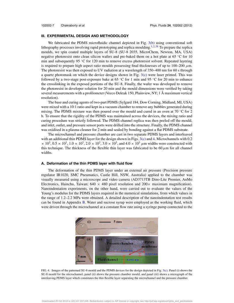
The microchannel and pressure chamber are cast in two separate PDMS layers and interleavedwith an additional thin PDMS layer for the design shown in Figs. 3(c) and 4. Microchannels with 0.2× 103, 0.5 × 103, 1.0 × 103, 2.0 × 103, 3.0 × 103, and 4.0 × 103 μm widths were constructed withthis technique. The thickness of the flexible thin layer was fabricated to be 60 μm for all channelwidths.

A. Deformation of the thin PDMS layer with fluid flow

The deformation of the thin PDMS layer under an external air pressure (Precision pressureregulator IR1020, SMC Pneumatics, Castle Hill, NSW, Australia) applied to the chamber wasvisually measured using a microscope and video camera (AD3713TB Dino-Lite Premier, AnMoElectronics, Hainchu, Taiwan; 640 × 480 pixel resolution and 200× maximum magnification).Nanoindentation experiments, on the other hand, were carried out to evaluate the values of theYoung’s modulus for the PDMS layers required in the numerical simulations, from which values inthe range of 1.2–2.2 MPa were obtained. A detailed description of the nanoindentation test resultscan be found in Appendix B. Water and sucrose syrup were employed as the working fluid, whichwere driven through the microchannel at a constant flow rate using a syringe pump connected to the

FIG. 4. Images of the patterned SU-8 mould and the PDMS devices for the design depicted in Fig. 3(c). Panel (i) shows theSU-8 mould for the microchannel, panel (ii) shows the pressure chamber mould, and panel (iii) shows a micrograph of theinterleaving PDMS layer which constitutes the thin flexible layer separating the microchannel and the pressure chamber.

Downloaded 20 Oct 2012 to 122.107.237.249. Redistribution subject to AIP license or copyright; see http://pof.aip.org/about/rights_and_permissions

102002-8 Chakraborty et al. Phys. Fluids 24, 102002 (2012)

channel inlet. To measure the pressure drop in the channel, we vertically mount capillary tubes atthe inlet and outlet, as illustrated in Fig. 1, and determine the difference in the height across the fluidcolumns in the capillary tubes.

IV. RESULTS AND DISCUSSION

A. Comparison between the two- and three-dimensional models in the absence of flow

Figure 5(a) depicts the maximum deformation predicted by the two-dimensional and three-dimensional ANSYS simulations (2D/3D-ANSYS) described in Sec. II B, showing that the two-dimensional model begins to deviate from the three-dimensional prediction once the width of thethin layer decreases below 2L, at which point boundary effects associated with edge pinning on bothsides can no longer be neglected. This is consistent with what we observe in the experiments wherewe measure the deformation of the thin PDMS layer under an external air pressure loading in theabsence of fluid flow. Figure 6(a) shows the deformed shape of the thin layer under an externallyapplied pressure. The maximum deformation of the thin layer, measured at the lowest point of theinflexion of its lower surface, is extracted visually from similar micrographs and shown in Fig. 6(b)as a function of the applied external pressure for microchannels of different widths. The experimentaldata point presented is the statistical average of at least five values, with vertical bars indicatingthe range of the deviation; probable sources of the experimental error are the manual handling ofthe microscope and video camera, visual image analysis to extract the deformed shape of the thinlayer, and manual measurement of the fluid column height in the capillary tubes. In agreement withthe predictions of the numerical simulations, we see that the deformation becomes independent ofthe microchannel (and thin layer) width when it exceeds 2L, therefore suggesting that boundaryeffects associated with the thin layer pinning at the lateral edges in a three-dimensional modelcan be neglected and a two-dimensional (infinite width) approximation suffices beyond this criticaldimension.

The validity of the two-dimensional incompressible neo-Hookean model (i.e., 2D-FEM-FSI) isfurther verified against experimental data for microchannels with large widths above 2L. Figure 5(b)shows a comparison between the maximum deformation measured in the experiments and thosepredicted by the two-dimensional model, from which we observe agreement with the experimental

FIG. 5. (a) Maximum deformation of the lower surface of the thin flexible layer �zmax as a function of its width Wfor three different values of the applied external pressure pe, as predicted by the 3D-ANSYS simulation described inSec. II B. The solid lines were added to aid visualisation. Also shown by the dashed lines are the results of a 2D-ANSYS(infinite width assumption) finite element simulation, indicating the diminishing effect of boundary effects associated withthe pinned lateral edges in the three-dimensional model above a width of approximately 2 × 103 μm. (b) Comparisonof experimental results with the two-dimensional simulation (2D-FEM-FSI), confirming the two-dimensional simulation,beyond a critical width, is an adequate approximation for capturing the deformation behaviour observed in the experiments.Since PDMS has a curing-dependent (and therefore thickness-dependent) Young’s modulus, different values of the Young’smodulus have been used in the simulations.

Downloaded 20 Oct 2012 to 122.107.237.249. Redistribution subject to AIP license or copyright; see http://pof.aip.org/about/rights_and_permissions

102002-9 Chakraborty et al. Phys. Fluids 24, 102002 (2012)

FIG. 6. (a) Micrograph showing the deformation of the thin flexible PDMS layer under the application of an external pressurepe of 20 kPa for the microchannel designs shown in Fig. 3(b) with a channel width of approximately 0.5 × 103 μm. (b)Maximum deformation of the thin layer �zmax, measured at the lowest point of the inflexion of its lower surface, as a functionof the externally applied pressure for microchannels with varying widths.

data to be bounded by the numerical predictions using two values of Young’s modulus for the thinlayer. We note that the large deformation data are well predicted by a lower value of the Young’smodulus whereas better agreement with the small deformation data is captured using a largervalue. Both lower and upper values however fall within the 1.2–2.2 MPa range measured using thenanoindentation technique described in Appendix B. In any case, the result provides further evidenceto suggest that the two-dimensional model is sufficient to capture the thin layer deformation when itis beyond a critical value of 2L, which is consistently predicted by both experiment and simulation.

B. Flow experiments: Pressure drop and thin layer deformation

Figure 7 shows the pressure drop �p as a function of the flow rate Q obtained from bothexperimental measurements and that predicted by the finite element model (2D-FEM-FSI) describedin Sec. II A; the pressure drop measurements were carried out in the absence of an external pressure.Also shown is the pressure drop and flow rate relationship for two-dimensional fully developedviscous flow through a long and rigid rectangular microchannel, for which it is possible to obtain ananalytical solution if the channel height H and width W are small compared to the channel length

0 10 200

35

70

Q (ml/hr)

Δ p

(mm

of

wat

er)

ExperimentalW = 0.5 LW = 3 LAnalyticalW = 0.5 LW = 3 L2D−FEM−FSI

FIG. 7. Relationship between the pressure drop �p and flow rate Q across a deformable microchannel with two differentchannel widths. It can be seen that the experimental observations (symbols) match well with the predictions afforded by thefinite element simulation (i.e., 2D-FEM-FSI) described in Sec. II A (dashed line) and that for a rigid rectangular microchannel(Eq. (15); solid line). For the narrower channel, however, we observe that the analytical solution for the rigid microchanneloverpredicts the pressure drop at higher flow rates. In all of these cases, there is no applied external pressure, i.e. pe = 0.

Downloaded 20 Oct 2012 to 122.107.237.249. Redistribution subject to AIP license or copyright; see http://pof.aip.org/about/rights_and_permissions

102002-10 Chakraborty et al. Phys. Fluids 24, 102002 (2012)

L—the solution for the longitudinal velocity takes the form39

vx = 4H 2�p

π3ηL

∞∑n,odd

1

n3

[1 − cosh(nπy/H )

cosh(nπW/2H )

]sin

(nπ z

H

). (14)

Integrating along the width and height of the channel then gives the required pressure drop and flowrate relationship

Q = H 3W�p

12ηL

[1 −

∞∑n,odd

192H

n5π5Wtanh

(nπW

2H

)]. (15)

The exact analytical solutions reported in Eqs. (14) and (15) are only valid when the channel is rigidand the cross section of the channel does not vary along its length, when the width of the channelis much greater than its height, and when the Reynolds number is very low (Re � 1) such thatinertial effects can be neglected. The experimental pressure drop and flow rate relationship werein good agreement with those predicted by the analytical solution for a rigid microchannel andthe 2D-FEM-FSI for the case of the wide channel. This further suggests that the two-dimensionalmodel constitutes a good approximation when the channel, and hence the thin layer, is sufficientlywide, such that three-dimensional effects (for instance, the pinned boundaries at the sidewalls) canbe neglected. The good agreement with the analytical solution, which does not account for the thinflexible layer, also suggests that the effect of the deformation on the pressure drop is small, andhence can be neglected. This is, however, not true for the case of small channel widths in which weobserve a departure from the rigid channel prediction at larger flow rates. The cross-sectional areafor a 0.5L width channel is much lower than that for a 3L width channel, and hence the pressuredrop is intuitively expected to be higher in the narrower channel for a specified flow rate. However,due to the flexibility of the PDMS channel, we observe some deformation of the channel wall dueto the increased fluid stresses at the higher flow rate. This deformation increases the effective cross-sectional area, leading to a reduction in the observed pressure drop. Clearly, the analytical solutionfor the rigid microchannel cannot account for this deformation, and consequently overpredicts thepressure drop.

Figure 8(a) shows profiles of the deformed thin layer shape under a specified external pressurefor varying flow rates (and hence corresponding average inlet velocities U0), as predicted by the2D-FEM-FSI simulation described in Sec. II A. We observe no significant deformation of the thinlayer below U0 = 5 × 10−2 m/s corresponding to a flow rate of Q = 110 ml/h. This is confirmed inour experiments where we do not observe any measurable changes in the thin layer shape at these

FIG. 8. Shape of the thin layer profile as predicted by the finite element model (i.e., 2D-FEM-FSI) described in Sec. II Afor varying (a) average inlet velocity and (b) fluid viscosity. The rest of the parameters used in the simulation arepe = 8 kPa, E = 1.95 MPa, t = 60 μm, H = 200 μm, and W = 3 × 103 μm. In (a), the Reynolds number is in therange 0–200 and η = 0.001 Pa s, whereas in (b), the Reynolds number is in the range 0.01–0.1 with U0 = 5 × 10−3 m/s.

Downloaded 20 Oct 2012 to 122.107.237.249. Redistribution subject to AIP license or copyright; see http://pof.aip.org/about/rights_and_permissions

102002-11 Chakraborty et al. Phys. Fluids 24, 102002 (2012)

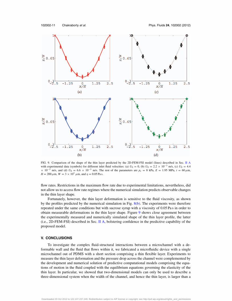
FIG. 9. Comparison of the shape of the thin layer predicted by the 2D-FEM-FSI model (lines) described in Sec. II Awith experimental data (symbols) for different inlet fluid velocities: (a) U0 = 0, (b) U0 = 2.2 × 10−3 m/s, (c) U0 = 4.4× 10−3 m/s, and (d) U0 = 6.6 × 10−3 m/s. The rest of the parameters are pe = 8 kPa, E = 1.95 MPa, t = 60 μm,H = 200 μm, W = 3 × 103 μm, and η = 0.05 Pa s.

flow rates. Restrictions in the maximum flow rate due to experimental limitations, nevertheless, didnot allow us to access flow rate regimes where the numerical simulation predicts observable changesin the thin layer shape.

Fortunately, however, the thin layer deformation is sensitive to the fluid viscosity, as shownby the profiles predicted by the numerical simulation in Fig. 8(b). The experiments were thereforerepeated under the same conditions but with sucrose syrup with a viscosity of 0.05 Pa s in order toobtain measurable deformations in the thin layer shape. Figure 9 shows close agreement betweenthe experimentally measured and numerically simulated shape of the thin layer profile, the latter(i.e., 2D-FEM-FSI) described in Sec. II A, bolstering confidence in the predictive capability of theproposed model.

V. CONCLUSIONS

To investigate the complex fluid-structural interactions between a microchannel with a de-formable wall and the fluid that flows within it, we fabricated a microfluidic device with a singlemicrochannel out of PDMS with a short section comprising a thin flexible layer. Experiments tomeasure the thin layer deformation and the pressure drop across the channel were complemented bythe development and numerical solution of predictive computational models comprising the equa-tions of motion in the fluid coupled with the equilibrium equations governing the elasticity of thethin layer. In particular, we showed that two-dimensional models can only be used to describe athree-dimensional system when the width of the channel, and hence the thin layer, is larger than a

Downloaded 20 Oct 2012 to 122.107.237.249. Redistribution subject to AIP license or copyright; see http://pof.aip.org/about/rights_and_permissions

102002-12 Chakraborty et al. Phys. Fluids 24, 102002 (2012)

critical dimension, in our case 2L, such that boundary effects arising from the pinning of the thinlayer to the channel walls at its lateral edges can be neglected—a threshold predicted by the simu-lation that agrees well with our experimental observations. In addition, we find excellent agreementbetween the predictions of the deformed thin layer shape under an externally applied air pressureusing both two-dimensional and three-dimensional models with that measured in the experiments.We believe that the combination of these results, the predictive capability of the numerical modelsdeveloped, and the physical insight gleaned in this study would be useful in the design of polymer-based microfluidic devices, and in particular, microactuation schemes such as the pneumaticallydriven micropumps, micromixers, microvalves, and microfilters employing thin flexible polymerlayers that have grown increasingly popular over the last decade.

ACKNOWLEDGMENTS

We thank Matteo Pasquali and Marcio Carvalho for providing us with their finite element codefor simulating coating flows, which we have modified and adapted to this work. This work wassupported by an award under the Merit Allocation Scheme on the NCI National Facility at theAustralian National University (ANU). The authors would also like to thank VPAC (Australia) andSUNGRID (Monash University, Australia) for the allocation of computing time on their supercom-puting facilities. L.Y. is supported by an Australian Research Fellowship awarded by the AustralianResearch Council under Discovery Project Grant No. DP0985253. J.R.F. is grateful for the MCNTech Fellowship from the Melbourne Centre for Nanofabrication and the Vice-Chancellor’s SeniorResearch Fellowship from RMIT University, and acknowledges partial support of this work from theAustralian Research Council Grant No. DP120100013 and the use of MCN facilities for fabricationof the structures reported in this study.

APPENDIX A: WEIGHTED RESIDUAL FORM OF THE EQUILIBRIUM EQUATION∇X · S = 0

Here, we provide a correction to the weighted residual form of the equilibrium equation givenby Eq. (4) derived by Carvalho and Scriven.29 The error in the original derivation, while insignificantfor small deformations, leads to significant discrepancies when the deformation is large.

The weak form of Eq. (4) is∫�S

(∇X · S) φ d�S = −∫

�S

(∇Xφ · S) d�S +∫

S

φ (N · S) dS = 0, (A1)

where �S , S , and N are the area, arc length, and unit normal in the zero-stress configuration,respectively, and φ is a weighting function. When written in terms of Cartesian components, theweighted residual form of this equation in the computational domain is

Rxi = −

∫�S0

[∂φi

∂ XSX x + ∂φi

∂YSY x

]|J∗| d�S0 +

∫S0

φi (N · S)x

(dS

dS0

)dS0, (A2)

Ryi = −

∫�S0

[∂φi

∂ XSX y + ∂φi

∂YSY y

]|J∗| d�S0 +

∫S0

φi (N · S)y

(dS

dS0

)dS0. (A3)

Here, �S0 and S0 are the area and arc length in the computational domain, respectively, |J∗| isthe Jacobian of the transformation from the zero-stress configuration to the computational domainand φi is a bi-quadratic weighting function. The components of the dimensional Piola-Kirchhoffstress tensor S, in terms of the dimensional Cauchy stress tensor for a neo-Hookean materialσ = −π∗ I + G B, are

SX x = −π∗ ∂y

∂Y+ G

∂x

∂ X, SY x = π∗ ∂y

∂ X+ G

∂x

∂Y,

SX y = π∗ ∂x

∂Y+ G

∂y

∂ X, SY y = −π∗ ∂x

∂ X+ G

∂y

∂Y,

(A4)

Downloaded 20 Oct 2012 to 122.107.237.249. Redistribution subject to AIP license or copyright; see http://pof.aip.org/about/rights_and_permissions

102002-13 Chakraborty et al. Phys. Fluids 24, 102002 (2012)

FIG. 10. Geometry of the solid domain of a beam fixed at the edges with uniform pressure applied on both the top andbottom of the beam.

where I is the identity tensor, π* is a pressure-like scalar function and B is the left Cauchy-Greentensor. In their finite element formulation of the fluid-structure interaction problem, Carvalho andScriven29 (see also Carvalho40) have used

Rxi = −

∫�S0

[SX x

∂φi

∂ X+ SX y

∂φi

∂Y

]|J∗| d�S0 +

∫S0

φi (N · S)x

(dS

dS0

)dS0 (A5)

and

Ryi = −

∫�S0

[SY x

∂φi

∂ X+ SY y

∂φi

∂Y

]|J∗| d�S0 +

∫S0

φi (N · S)y

(dS

dS0

)dS0 (A6)

in place of Eqs. (A2) and (A3). Essentially, the positions of the two components SYx and SXy havebeen interchanged.

In order to establish the validity of Eqs. (A2) and (A3) and to demonstrate the incorrectnessof Eqs. (A5) and (A6), we have examined the simple problem of a beam fixed at the edges withuniform pressure applied on both the top and bottom of the beam, as shown schematically inFig. 10. Essentially, we compare the results of our computation using Eqs. (A2) and (A3) (labelledFEM-N), and Eqs. (A5) and (A6) (labelled FEM-C), with the results obtained with the finite elementANSYS simulation for a plane-strain model described in Sec. II B. In addition, we prescribe boundaryconditions in the form of zero displacement along the left and right edges of the beam, and a forcebalance at the top and bottom of the form

n · σ = −pi n (i = 1, 2), (A7)

where n is the unit normal to the deformed solid surface, and p1 and p2 are the dimensional externalpressures on the top and bottom of the beam, respectively.

In units of height H, the length of the beam is set at L = 5H, with H = 10−3 m. The externalpressures have been chosen to be p1 = 1.1 N and p2 = 1.0 N, and three different values (6000,12 000, and 24 000 Pa) have been used for the shear modulus G. Computations have been performedwith three different meshes (M1, M2, and M3) in order to examine mesh convergence. We notethat the formulation of the fluid-structure interaction problem by Carvalho and Scriven29 appliesto the special case of an incompressible neo-Hookean material with a Poisson ratio ν = 0.5. Onthe other hand, the ANSYS plane-strain package fails for an incompressible neo-Hookean material.Consequently, in order to carry out the comparison with the ANSYS simulations, we have obtainedpredictions with several values of ν < 0.5, and extrapolated the results to ν = 0.5.

Figure 11 compares the maximum displacement of the beam obtained with the FEM-N andFEM-C formulations with the ANSYS plane-strain model for the three different values of G. In allthree cases, mesh-converged results obtained with FEM-N are observed to agree with the extrapolatedmesh converged solution obtained with ANSYS. On the other hand, the mesh converged solutionobtained with FEM-C shows differences from the other two approaches. Indeed, while this differenceis small at G = 24 000 Pa, and substantially larger at G = 12 000 Pa, we are unable to obtain aconverged solution with FEM-C at G = 6000 Pa.

Downloaded 20 Oct 2012 to 122.107.237.249. Redistribution subject to AIP license or copyright; see http://pof.aip.org/about/rights_and_permissions

102002-14 Chakraborty et al. Phys. Fluids 24, 102002 (2012)

G

G

G

(a)

(c)

(b)

FIG. 11. Comparison between the results for maximum deformation from the FEM-N and FEM-C models with the ANSYSplane-strain model for three different values of G: (a) 24 000 Pa, (b) 12 000 Pa, and (c) 6000 Pa.

APPENDIX B: NANOINDENTATION CHARACTERISATION OF THE ELASTIC MODULUSOF THE THIN PDMS LAYER

Since the Young’s modulus of PDMS can be significantly altered by varying the curing temper-ature and time,41 and the mixing ratio of the silicone base to the curing agent,2, 8–10 there is a need tomeasure the isotropic mechanical properties of PDMS.42–44 Different experimental techniques havebeen employed to characterise the rigidity of PDMS and the reported value of Young’s modulus forPDMS usually falls within the range of 0.05–4.0 MPa.8, 9 Recently, Liu et al.42 have conducted a

Downloaded 20 Oct 2012 to 122.107.237.249. Redistribution subject to AIP license or copyright; see http://pof.aip.org/about/rights_and_permissions

102002-15 Chakraborty et al. Phys. Fluids 24, 102002 (2012)

tensile test to establish the thickness-dependent hardness and the Young’s modulus of thin PDMSlayers, arising due to the shear stresses that are exerted during fabrication of these thin layers. On theother hand, nanoindentation testing, which has been widely employed for characterising the elasticand plastic properties of hard materials, is also now being recognised as a tool for characterising themechanical properties of polymeric materials. In a standard nanoindentation test, the Young’s mod-ulus and hardness of a very thin layer made of elastic material can easily be obtained from the loaddisplacement data. Carrillo et al.,45 for example, used a nanoindentation technique to characterisethe Young’s modulus of PDMS with different degrees of crosslinking.

Here, PDMS (Dow and Corning Sylgard 184) samples were prepared by mixing the cross-linkerand siloxane in a ratio of 1:10, and subsequently kept in a vacuum chamber to remove the bubblesthat were generated during mixing. Thin PDMS layers with different thicknesses were then producedby spin coating glass wafers at various rotation speeds followed by curing in an oven at 70 ◦C for 2 h.The thickness of the thin PDMS layer was measured using a surface profiler. By varying the rotationspeed of the spin coating process between 500 and 2000 rpm, thin PDMS layers of thicknesses inthe range of 25 μm to 100 μm were produced.

The nanoindentation testing is carried out using a TriboIndenter R© (Hysitron, Inc., Minneapolis,MN, USA) with a Berkovich indenter tip at room temperature. For load control function, we employa loading and unloading rate of 10 μN/s, peak load of 100 μN, and a hold period of 5 s. When the tipof the indentor reaches the sample surface, the instrument applies the predefined load and recordsthe load and displacement data accordingly. The hardness and the Young’s modulus of the material isthen determined from the unloading portion of the load-displacement curve using classical Hertziancontact theory,46

H = Fmax

A, (B1)

1

Er= 1 − ν2

E+ 1 − ν2

i

Ei, (B2)

where H is the hardness of the substrate and Fmax is the maximum force applied on the PDMS layer.A is the projected contact area between the tip and the substrate, ν and E are the Poisson’s ratio andthe Young’s modulus for the test specimen, respectively, and ν i and Ei are those for the indenter. Thematerial properties of the diamond indenter are Ei = 1140 GPa and ν i = 0.07. The reduced elasticmodulus Er is calculated using the following expression proposed by Oliver and Pharr:47

Er = S√

π

2β√

A, (B3)

where S is the contact stiffness, taken as the initial slope of the unloading section of the load-displacement curve, and β is a constant that depends on the geometry of the indenter.

Figure 12(a) shows the indentor displacement in response to the applied load during a nanoin-dentation test carried out on the thin PDMS layer using quasi-static measurements. To confirm thereproducibility of the test data, the indentation is performed on nine different locations of a givensample. The penetration depth of the indenter is observed to be higher for thinner layers, indicatinga lower value for the Young’s modulus as the thickness decreases. Similar trends are also observedfor other thin PDMS layers.

The reduced elastic modulus Er and Young’s modulus of the thin PDMS layer are calculatedusing Eqs. (B2) and (B3). Figure 12(b) further indicates that the Young’s modulus of the PDMSlayers decreases with decreasing thicknesses. This is a consequence of the polymer moleculesexperiencing enhanced radial stretching due to an increase in the shear stress with the increasingspinning speeds that are required to produce thinner layers. In any case, the good agreement betweenthe measured values for the Young’s modulus therefore suggest that the nanoindentation test iscapable of differentiating the elastic behaviour of a polymeric material with varying thickness.

Downloaded 20 Oct 2012 to 122.107.237.249. Redistribution subject to AIP license or copyright; see http://pof.aip.org/about/rights_and_permissions

102002-16 Chakraborty et al. Phys. Fluids 24, 102002 (2012)

FIG. 12. (a) Load-displacement curves for a thin PDMS layer with a thickness of 0.05 mm. (b) Thickness dependence of thereduced elastic modulus Er and Young’s modulus E of the PDMS layer.

APPENDIX C: VALIDATION OF THE FINITE ELEMENT FORMULATION

Here, we briefly provide results on the validation of the finite element formulation described inSec. II B against simple benchmark cases that have been reported earlier in the literature.

1. Couette flow past a finite thickness solid

The flow of a Newtonian fluid past an incompressible neo-Hookean solid, as shown schemati-cally in Fig. 13, has been previously described by Gkanis and Kumar.48 The interface between thefluid and solid is located at y = t and a rigid plate located at z = (H + t) moves in the x directionat a constant speed U0, giving rise to Couette flow in the fluid domain; the bottom edge of the solidis held fixed. Gkanis and Kumar48 performed a linear stability analysis of this problem in the limitof zero Reynolds number Re and infinite domain length L, and have shown that the steady-statesolution of the deformation in the solid produced by the Couette flow is

x = (x, y) = (X + Y, Y ), (C1)

where = (ηU0)/(GH) is a dimensionless number.Computations have been performed to compare predictions for the deformation of the solid

domain at L/2 with the analytical results of Gkanis and Kumar.48 In order to eliminate end effectscaused by the fixed ends of the solid and fluid domains in the computations, we have varied thelength of the domain between 10 and 30 m and ensured that domain length independent predic-tions are obtained. The following parameter values have been used: ρ = 10−3 kg/m3, η = 1 Pa s,H = 1 m, t = 1 m, and U0 = 1 × 10−3–1.75 × 10−3 m/s (such that Re ∼ 0) and G = 10−2 Pa. Thechoice of these parameter values maintains in the range 0.1–0.175. The mid-surface displacementof the solid predicted by the finite element formulation is compared with the analytical solution

FIG. 13. Schematic depiction of Couette flow of a Newtonian fluid past an incompressible finite thickness neo-Hookeansolid.

Downloaded 20 Oct 2012 to 122.107.237.249. Redistribution subject to AIP license or copyright; see http://pof.aip.org/about/rights_and_permissions

102002-17 Chakraborty et al. Phys. Fluids 24, 102002 (2012)

0 0.5 10

0.05

0.1

0.15

Thickness of the solid ( t/W)

Mid

sur

face

dis

plac

emen

t

Γ=0.1Γ=0.125Γ=0.15Γ=0.175

FIG. 14. Comparison of the finite element simulation with the analytical solution for different values of . The lines denotethe analytical solution reported by Gkanis and Kumar48 whereas symbols are the predictions from our simulation.

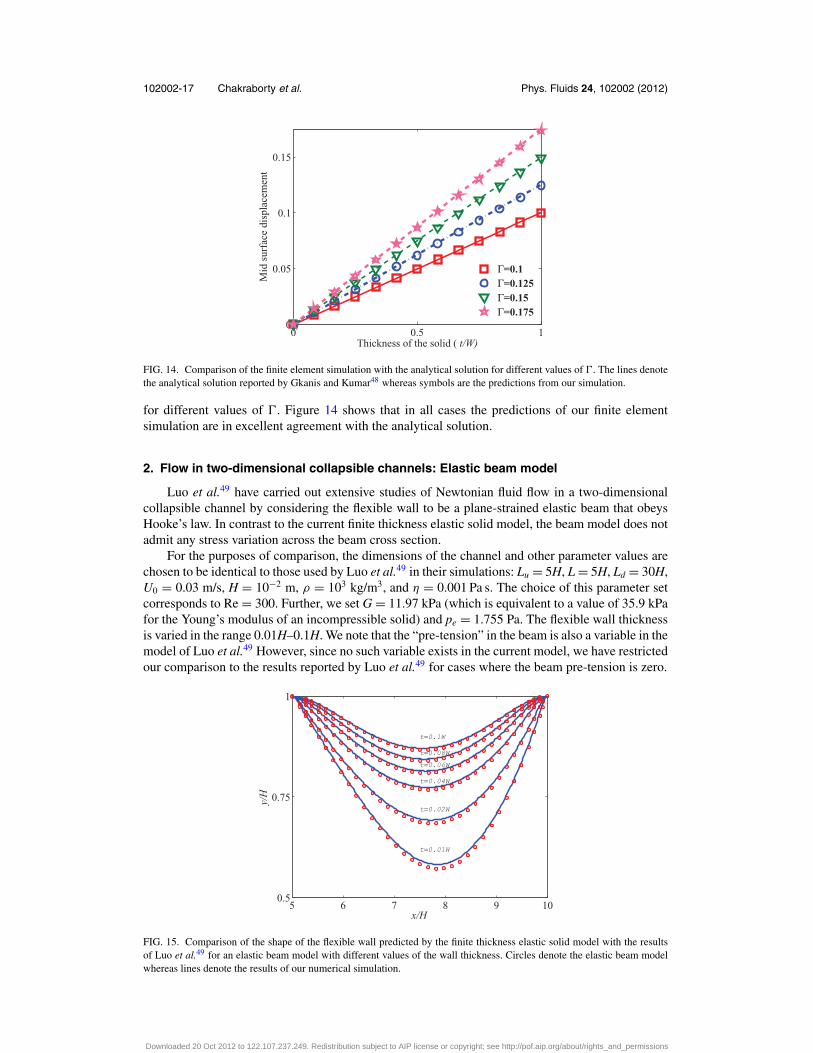
for different values of . Figure 14 shows that in all cases the predictions of our finite elementsimulation are in excellent agreement with the analytical solution.

2. Flow in two-dimensional collapsible channels: Elastic beam model

Luo et al.49 have carried out extensive studies of Newtonian fluid flow in a two-dimensionalcollapsible channel by considering the flexible wall to be a plane-strained elastic beam that obeysHooke’s law. In contrast to the current finite thickness elastic solid model, the beam model does notadmit any stress variation across the beam cross section.

For the purposes of comparison, the dimensions of the channel and other parameter values arechosen to be identical to those used by Luo et al.49 in their simulations: Lu = 5H, L = 5H, Ld = 30H,U0 = 0.03 m/s, H = 10−2 m, ρ = 103 kg/m3, and η = 0.001 Pa s. The choice of this parameter setcorresponds to Re = 300. Further, we set G = 11.97 kPa (which is equivalent to a value of 35.9 kPafor the Young’s modulus of an incompressible solid) and pe = 1.755 Pa. The flexible wall thicknessis varied in the range 0.01H–0.1H. We note that the “pre-tension” in the beam is also a variable in themodel of Luo et al.49 However, since no such variable exists in the current model, we have restrictedour comparison to the results reported by Luo et al.49 for cases where the beam pre-tension is zero.

5 6 7 8 9 100.5

0.75

1

x/H

y/H

t=0.1W

t=0.08W

t=0.06W

t=0.04W

t=0.02W

t=0.01W

FIG. 15. Comparison of the shape of the flexible wall predicted by the finite thickness elastic solid model with the resultsof Luo et al.49 for an elastic beam model with different values of the wall thickness. Circles denote the elastic beam modelwhereas lines denote the results of our numerical simulation.

Downloaded 20 Oct 2012 to 122.107.237.249. Redistribution subject to AIP license or copyright; see http://pof.aip.org/about/rights_and_permissions

102002-18 Chakraborty et al. Phys. Fluids 24, 102002 (2012)

FIG. 16. (a) Extrapolation to t = 0 of the flexible wall shape obtained from the finite thickness elastic solid model fort = 0.01H, t = 0.05H, and t = 0.1H. (b) Comparison of the shape of the flexible wall predicted by the finite-thickness solidmodel (symbols) with the prediction of the zero-thickness thin layer model (solid line). (c) Extrapolation of the averagetension acting in the elastic solid to the limit of zero wall thickness.

Downloaded 20 Oct 2012 to 122.107.237.249. Redistribution subject to AIP license or copyright; see http://pof.aip.org/about/rights_and_permissions

102002-19 Chakraborty et al. Phys. Fluids 24, 102002 (2012)

Figure 15 shows a comparison between the prediction of the shape of the flexible wall of ourfinite thickness elastic solid model and that reported by Luo et al.49 While our simulations agreewith Luo et al.49 for the relatively small deformations that occur at large thin layer thicknessest, the Hookean beam model, as expected, begins to depart from the prediction of the nonlinearneo-Hookean model for large deformations that are associated with small thin layer thicknesses.

3. Flow in two-dimensional collapsible channels: Zero-thickness thin layer model

Simulations have also been performed to compare predictions of the flexible wall shape fromthe current finite thickness elastic solid model with the zero-thickness thin layer model of Luo andPedley23 for the flow of a Newtonian fluid. Apart from the simplicity of the zero-thickness thin layermodel from a constitutive point of view, a fundamental difference between the two models is thatwhile the tension in the flexible wall is prescribed a priori in the zero-thickness thin layer model, itis part of the solution in the finite thickness elastic solid model. As a result, a multi-step procedureis required to carry out the comparison, as described in the paragraphs to follow.

The zero-thickness thin layer model is first computed for a pre-determined value of thinlayer tension equal to 675 N/m, with the following parameter values: Re = 1, ρ = 1054 kg/m3,U0 = 1.338 × 10−2 m/s, H = 10−2 m, η = 0.141 Pa s, and pe = 17 545 N/m2. This leads to aprediction of the minimum height of the gap in the channel (beneath the flexible thin layer) of h/H= 0.125. Computations with the finite thickness elastic solid model are then carried out for the sameparameter values, for various combinations of the flexible wall thickness t and shear modulus G suchthat each combination always leads to the same value of the minimum channel gap height, namely,h/H = 0.125. It turns out that even though the minimum gap height is the same in both models, thepredicted interface shape is not, with the difference increasing as the thickness of the elastic solidincreases. This is clearly a result of the finite thickness of the elastic solid. Consequently, in orderto compare the interface shape, we carry out an extrapolation procedure in which the height of theinterface at various locations in the gap as a function of the flexible wall thickness is extrapolatedto the limit of zero wall thickness, as shown in Fig. 16(a). The extrapolated interface shape is thencompared with the prediction by the zero-thickness thin layer model in Fig. 16(b), in which weobserve excellent agreement between the two models.

The remaining step involves the evaluation of the resultant tension in the finite thickness elasticsolid and how it compares with the pre-determined thin layer tension of 675 N/m. Here, we firstestimate the tension in the finite thickness solid at a particular location x by averaging the tangentialsolid stresses acting across the cross section at x. An estimate of the overall tension in the solid isthen obtained by averaging the tension along the entire length of the flexible solid for all valuesof x. The values of the average tension obtained from the finite thickness elastic solid model fort = 0.01H, t = 0.05H, and t = 0.1H are then extrapolated to t = 0, as shown in Fig. 16(c), in whichwe observe the extrapolated value of tension to be fairly close to the value of 675 N/m used in thezero-thickness thin layer model.

1 J. M. K. Ng, I. Gitlin, A. D. Stroock, and G. M. Whitesides, “Components for integrated poly(dimethylsiloxane) microfluidicsystems,” Electrophoresis 23, 3461–3473 (2002).

2 J. Friend and L. Yeo, “Fabrication of microfluidic devices using polydimethylsiloxane,” Biomicrofluidics 4, 026502 (2010).3 L. Y. Yeo, H.-C. Chang, P. P. Y. Chan, and J. R. Friend, “Microfluidic devices for bioapplications,” Small 7, 12–48 (2011).4 T. Vestad, D. W. M. Marr, and J. Oakey, “Flow control for capillary-pumped microfluidic systems,” J. Micromech.

Microeng. 14, 1503–1506 (2004).5 C. H. Wang and G. B. Lee, “Pneumatically driven peristaltic micropumps utilizing serpentine-shape channels,” J. Mi-

cromech. Microeng. 16, 341–348 (2006).6 D. Irimia and M. Toner, “Cell handling using microstructured membranes,” Lab Chip 6, 345–352 (2006).7 S.-B. Huang, M.-H. Wu, and G.-B. Lee, “A tunable micro filter modulated by pneumatic pressure for cell separation,”

Sens. Actuators B 142, 389–399 (2009).8 A. L. Thangawng, R. S. Ruoff, M. A. Swartz, and M. R. Glucksberg, “An ultra-thin PDMS membrane as a bio/micronano

interface: Fabrication and characterization,” Biomed. Microdevices 9, 587–595 (2007).9 D. Fuard, T. Tzvetkova-Chevolleau, P. T. S. Decossas, and P. Schiavone, “Optimization of poly-di-methyl-siloxane (PDMS)

substrates for studying cellular adhesion and motility,” Microelectron. Eng. 85, 1289–1293 (2008).10 D. N. Hohne, J. G. Younger, and M. J. Solomon, “Flexible microfluidic device for mechanical property characterization of

soft viscoelastic solids such as bacterial biofilms,” Langmuir 25, 7743–7751 (2009).

Downloaded 20 Oct 2012 to 122.107.237.249. Redistribution subject to AIP license or copyright; see http://pof.aip.org/about/rights_and_permissions

102002-20 Chakraborty et al. Phys. Fluids 24, 102002 (2012)

11 M. A. Unger, H. P. Chou, T. Thorsen, A. Scherer, and S. R. Quake, “Monolithic microfabricated valves and pumps bymultilayer soft lithography,” Science 288, 113–116 (2000).

12 D. Irimia, S.-Y. Liu, W. Tharp, A. Samadani, M. Toner, and M. Poznansky, “Microfluidic system for measuring neutrophilmigratory responses to fast switches of chemical gradients,” Lab Chip 6, 191–198 (2006).

13 W. A. Conrad, “Pressure-flow relationships in collapsible tubes,” IEEE Trans. Bio-Med. Eng. 16, 284–295(1969).

14 R. W. Brower and C. Scholten, “Experimental evidence on the mechanism for the instability of flow in collapsible vessels,”Med. Biol. Eng. 13, 839–844 (1975).

15 C. D. Bertram, “Two modes of instability in a thick-walled collapsible tube conveying a flow,” J. Biomech. 15, 223–224(1982).

16 C. D. Bertram, “Unstable equilibrium behaviour in collapsible tubes,” J. Biomech. 19, 61–69 (1986).17 C. D. Bertram, “The effects of wall thickness, axial strain and end proximity on the pressure-area relation of collapsible

tubes,” J. Biomech. 20, 863–876 (1987).18 C. D. Bertram, C. J. Raymond, and T. J. Pedley, “Mapping of instabilities during flow through collapsed tubes of differing

length,” J. Fluids. Struct. 4, 125–153 (1990).19 C. D. Bertram, C. J. Raymond, and T. J. Pedley, “Application of non-linear dynamics concepts to the analysis of self-excited

oscillations of a collapsible tube conveying a flow,” J. Fluids. Struct. 5, 391–426 (1991).20 C. D. Bertram and S. A. Godbole, “LDA measurements of velocities in a simulated collapsed tube,” ASME J. Biomech.

Eng. 119, 357–363 (1997).21 C. D. Bertram and R. Castles, “Flow limitation in uniform thick-walled collapsible tubes,” J. Fluids Struct. 13, 399–418

(1999).22 C. D. Bertram and N. S. J. Elliott, “Flow-rate limitation in a uniform thin-walled collapsible tube, with comparison to a

uniform thick-walled tube and a tube of tapering thickness,” J. Fluids Struct. 17(4), 541–559 (2003).23 X. Y. Luo and T. J. Pedley, “A numerical simulation of steady flow in a 2-D collapsible channel,” J. Fluids Struct. 9,

149–174 (1995).24 X. Y. Luo and T. J. Pedley, “A numerical simulation of unsteady flow in a two-dimensional collapsible channel,” J. Fluid

Mech. 314, 191–225 (1996).25 A. L. Hazel and M. Heil, “Steady finite-Reynolds-number flows in three-dimensional collapsible tubes,” J. Fluid Mech.

486, 79–103 (2003).26 M. Heil and O. E. Jensen, “Flows in deformable tubes and channels—Theoretical models and biological applications,” in

Flow Past Highly Compliant Boundaries and in Collapsible Tubes, edited by P. W. Carpenter and T. J. Pedley (Kluwer,Dordrecht, 2003), pp. 15–50.

27 A. Marzo, X. Luo, and C. Bertram, “Three-dimensional collapse and steady flow in thick-walled flexible tubes,” J. Fluids.Struct. 20, 817–835 (2005).

28 H. F. Liu, X. Y. Luo, Z. X. Cai, and T. J. Pedley, “Sensitivity of unsteady collapsible channel flows to modellingassumptions,” Commun. Numer. Methods Eng. 25, 483–504 (2009).

29 M. S. Carvalho and L. E. Scriven, “Flows in forward deformable roll coating gaps: Comparison between spring and planestrain models of roll cover” J. Comput. Phys. 138, 449–479 (1997).

30 J. M. deSantos, “Two-phase cocurrent downflow through constricted passages,” Ph.D. dissertation (University of Minnesota,Minneapolis, MN, 1991).

31 K. N. Christodoulou and L. E. Scriven, “Discretization of free surface flows and other moving boundary problems,” J.Comput. Phys. 99, 39–55 (1992).

32 D. F. Benjamin, “Roll coating flows and multiple roll systems,” Ph.D. dissertation (University of Minnesota, Minneapolis,MN, 1994).

33 M. Pasquali and L. E. Scriven, “Free surface flows of polymer solutions with models based on the conformation tensor,”J. Non-Newtonian Fluid Mech. 108, 363–409 (2002).

34 G. A. Zevallos, M. S. Carvalho, and M. Pasquali, “Forward roll coating flows of viscoelastic liquids,” J. Non-NewtonianFluid Mech. 130, 96–109 (2005).

35 M. Bajaj, J. R. Prakash, and M. Pasquali, “A computational study of the effect of viscoelasticity on slot coating flow ofdilute polymer solutions,” J. Non-Newtonian Fluid Mech. 149, 104–123 (2008).

36 D. Chakraborty, M. Bajaj, L. Yeo, J. Friend, M. Pasquali, and J. R. Prakash, “Viscoelastic flow in a two-dimensionalcollapsible channel,” J. Non-Newtonian Fluid Mech. 165, 1204–1218 (2010).

37 ANSYS, Structural analyses guide, Mechanical APDL, Release 11.0, ANSYS, Inc., Canonsburg, PA, USA, 2010.38 D. C. Duffy, J. C. McDonald, O. J. A. Schueller, and G. M. Whitesides, “Rapid prototyping of microfluidic systems in

poly (dimethylsiloxane),” Anal. Chem 70, 4974–4984 (1998).39 N. Mortensen, F. Okkels, and H. Bruus, “Reexamination of Hagen-Poiseuille flow: Shape dependence of the hydraulic

resistance in microchannels,” Phys. Rev. E 71, 057301 (2005).40 M. S. Carvalho, “Roll coating flows in rigid and deformable gaps,” Ph.D. dissertation (University of Minnesota, Minneapo-

lis, MN, 1996).41 H. Schmid and B. Michel, “Siloxane polymers for high-resolution, high-accuracy soft lithography,” Macromolecules 33,

3042–3049 (2000).42 M. Liu, J. Sun, Y. Sun, C. Bock, and Q. Chen, “Thickness-dependent mechanical properties of polydimethylsiloxane

membranes,” J. Micromech. Microeng. 19, 035028 (2009).43 M. Liu, J. Sun, and Q. Chen, “Influences of heating temperature on mechanical properties of polydimethylsiloxane,” Sens.

Actuators A 151, 42–45 (2009).44 T. Kim, J. Kim, and O. Jeong, “Measurement of nonlinear mechanical properties of PDMS elastomer,” Microelectron.

Eng. 88, 1982–1985 (2011).

Downloaded 20 Oct 2012 to 122.107.237.249. Redistribution subject to AIP license or copyright; see http://pof.aip.org/about/rights_and_permissions

102002-21 Chakraborty et al. Phys. Fluids 24, 102002 (2012)

45 F. Carrillo, S. Gupta, M. Balooch, S. J. Marshall, G. W. Marshall, L. Pruitt, and C. Puttlitz, “Nanoindentation of poly-dimethylsiloxane elastomers: Effect of crosslinking, work of adhesion, and fluid environment on elastic modulus,” J. Mater.Res. 20, 2820–2830 (2005).

46 K. Johnson, Contact Mechanics (Cambridge University Press, Cambridge, 2003).47 W. C. Oliver and G. M. Pharr, “An improved technique for determining hardness and elastic modulus using load and

displacement sensing indentation experiments,” J. Mater. Res. 7, 1564–1583 (1992).48 V. Gkanis and S. Kumar, “Instability of creeping Couette flow past a neo-Hookean solid,” Phys. Fluids 15, 2864–2871

(2003).49 X. Y. Luo, B. Calderhead, H. F. Liu, and W. G. Li, “On the initial configurations of collapsible tube flow,” Comput. Struct.

85, 977–987 (2007).

Downloaded 20 Oct 2012 to 122.107.237.249. Redistribution subject to AIP license or copyright; see http://pof.aip.org/about/rights_and_permissions