fluid replacement model (frm) analysis of telisa sand
TRANSCRIPT

FLUID REPLACEMENT MODEL (FRM) ANALYSIS
OF TELISA SAND RESERVOIR : YM FIELD, SOUTH SUMATRA BASIN
THESIS
YOESE MARIAM
0706171636
PHYSICS GRADUATE PROGRAM FACULTY OF MATHEMATIC AND NATURAL SCIENCE
JAKARTA JULY, 2009
Fluid replacement..., Yoese Mariam, FMIPA UI, 2009

ii
PAGE OF APPROVAL
JUDUL : FLUID REPLACEMENT MODEL ANALYSIS OF TELISA SAND RESERVOIR : YM FIELD, SOUTH SUMATRA BASIN
NAMA : YOESE MARIAM NPM : 0706171636
APPROVED AS TO STYLE AND CONTENT BY :
Prof. Dr. Suprajitno Munadi Supervisor
Dr. Ricky Adi Wibowo Dr. Waluyo Dr. Abdul Haris Examiner Examiner Examiner
PHYSICS GRADUATE PROGRAM
FACULTY OF MATHEMATIC AND NATURAL SCIENCE
Dr. Dedi Suyanto
NIP. 130 935 271
Date of Final Examination : July 3, 2009
Fluid replacement..., Yoese Mariam, FMIPA UI, 2009

iii
Abstract
Rock physics data is a tool for fluid identification and quantification in reservoir, and also plays an important part in any fluid substitution study that may provide a valuable tool for modeling various fluid scenarios. This thesis presents the results of the two well cases where the effect of rock and fluid properties on seismic response are illustrated. Both of wells (YM-232 and YM-247) show the effect of replacing hydrocarbons with brine. This effectt illustrates how rock and fluid properties along with reflection amplitudes can be used to estimate fluid type in YM field. First synthetic using the original case. And the other synthetic by using FRM case, with an assumption that the fluid was brine/oil and the mineralogy was clean sand. These amplitude was extracted to be correlated with the real seismic data. Finally, a good correlation was obtain from a model to estimate the fluid type in prospect based on amplitude information in seismic data. In other word, we can understand the effect of hydrocarbon saturation on synthetic offset gathers. This analysis can be use as one of parameter to improve seismic 3D interpretation and to reduce drilling risk.
Abstrak
Data Rock Physics adalah alat untuk identifikasi fluida, perhitungan dalam reservoar, dan bagian penting dalam studi substitusi fluida untuk memodelkan berbagai macam fluida. Thesis ini merupakan hasil dari penelitian dua sumur untuk melihat pengaruh dari batuan dan properti fluida terhadap respon seismik. Kedua sumur tersebut adalah (YM-232 dan YM-247) merupakan oil well yang menunjukkan pengaruh dari substitusi hidrokarbon dengan air. Akibat dari substitusi fluida terhadap batuan dan properti fluida menunjukkan respon tertentu pada refleksi amplitude, variasi amplitude tersebut dapat digunakan sebagai guide untuk memperkirakan penyebaran jenis fluida pada lapangan YM. Pertama dengan melakukan sintetik pada keadaan insitu. Diikuti dengan sintetik pada kondisi tersaturasi (FRM), dengan manganggap bahwa fluida adalah air/minyak dan mineral adalah batu pasir bersih. Amplitude ini akan diekstrak untuk dikorelasikan dengan data seismic yang sebenarnya. Koefisian korelasi yang memiliki nilai tinggi (~1) dijadikan sebagai model untuk memprediksi tipe fluida pada area prospek yang didasarkan pada informasi amplitude dari data seismik. Dengan kata lain, kita dapat memahami efek dari saturasi hidrokarbon terhadap synthetic offset gathers. Analisis ini digunakan sebagai salahsatu parameter untuk mengembangkan interpretasi data seismic 3D & untuk menekan/mengurangi resiko pengeboran.
Fluid replacement..., Yoese Mariam, FMIPA UI, 2009

iv
Foreword
All prise be to ALLAH SWT for His blessing & mercy, so that I can
accomplish my thesis.
I sincerely thank my supervisor, Profesor Suprajitno Munadi, for his guidance and
his patience. The arguments with him helped me to clear my thoughts and
remember the concepts that I forgot. Without his insistence, I would not have gone
this far into FRM seismogram.
I also want to thank my friends for helping me and giving me helpful suggestions
and also the examiner team. The discussion with them is very helpful for my
progress.
Finally, the support of my parents should not be understated. Particularly, I
dedicated my thesis to my beloved mother for her patience and endless prayer.
Fluid replacement..., Yoese Mariam, FMIPA UI, 2009

v
Table of Contents
Page
Title page………………………………………………………………...
Approval page …………………………………......................................
Abstract ……...………………………………………………………….
Foreword ………………………………………………………………..
Table of Contents ……………………………………………………….
Table of figures..……………………………………………………….
Chapter 1. Introduction ………………………………………………
1.1. Background …………………………………………….
1.2. Objectives ………………………………………………
1.3. Study Area ……………………………………………..
Chapter II. Theoretical Background…………………………………
2.1. Regional Geology Setting……………………………….
2.1.1 Structure & Tectonic………………………………
2.1.2 Tectonostratigraphy……………………………….
2.2. Telisa Sandstone Characterizations……………………..
2.3. Rock Physics Theory……………………………………
2.3.1 Rock Physics Properties of Shaly Sand………….
2.4. Fluid Substitutiton – Gassmann…………………………
2.4.1 Rock Properties……………………………………
2.4.2 Using Gassmann’s Equation………………………
2.4.3 Porosity…………………………………………….
2.4.4 Fluid Properties……………………………………
2.4.5 Matrix Properties………………………………….
2.4.6 Frame Properties…………………………………
2.4.7 Calculating Velocities…………………………….
2.4.8 Dry Frame Bulk Modulus, K*……………………..
2.5. Effect of Fluid Saturation on Seismic Properties…………
2.6. Theoretical Model………………………………………..
2.6.1 Internal Consistency & Saturation Modeling……
Chapter III. Data and Methodology …………………………………
i
ii
iii
iv
v
vi
1
1
2
2
2
2
4
4
4
5
6
9
10
13
13
14
14
14
15
15
16
16
16
16
Fluid replacement..., Yoese Mariam, FMIPA UI, 2009

vi
3.1 Methodology…………………..………………………..
3.1.1 Fluid Substitution…………………………………
3.2 Data……………………………………………………..
3.3 Wavelet Extraction & Well Seismic Tie………………...
Chapter IV. Analysis and Interpretation ……………………………
4.1 Data Processing…………………………………………..
4.2 Sensitivity Analysis………………………………………
4.3 Fluid Substitution…………………………………………
4.4 Wavelet Extraction & Well Seismic Tie………………….
4.5 Rock Physics Analysis & Synthetic Offset Gathers………
4.5.1 The Analysis of The Telisa Sand Reservoir at YM-
232 Well…………………………………………...
4.5.2 The Analysis of The Telisa Sand Reservoir at YM-
247 Well…………………………………………..
4.6 Comparison between Model Amplitude & Real Seismic…
Chapter V. Conclusions & Recommendation……… ………………
References……………………………………………………..
17
20
20
21
22
22
25
25
26
35
36
35
46
58
69
71
Fluid replacement..., Yoese Mariam, FMIPA UI, 2009

vii
Table of Figures
Page
Figure 1.1. Map showing the area of the thesis in YM Block at South
Sumatra Basin
Figure 2.1. Stratigraphy of South Sumatra……………………………..
Figure 2.2. Lines of Vp vs Pore for Shales with varying silt content….
Figure 2.3 Pore & P-wave Velocity vs Clay Content for Shaly Sands &
Sandy Shales………………………………………………
Figure 3.1 Work Flowchart………..........................................................
Figure 4.1 Composite Log YM-232 Well……………………………..
Figure 4.2. Composite Log YM-247 Well……………………………..
Figure 4.3. Porosity vs Sw & Porosity vs Vclay at YM-232 Well……..
Figure 4.4. Porosity vs Sw & Porosity vs Vclay at YM-247 Well…….
Figure 4.5 Crossplot Gamma Ray vs VpVs_Ratio with Color Key
Gamma Ray………………………………………………..
Figure 4.6 Crossplot Gamma Ray vs VpVs_Ratio with Color Key
Porosity……………………………………………………
Figure 4.7 Crossplot Gamma Ray vs VpVs_Ratio with Color Key
Saturasi……………………………………………………
Figure 4.8 Fluid Substitution at YM-232 Well………………………...
Figure 4.9 Fluid Substitution at YM-247 Well………………………..
Figure 4.10 Frequency Dominant at 40 Hz & Wavelet Extraction……..
Figure 4.11 Correlation with Ricker 40 Hz at YM-232 Well…………...
Figure 4.12 Correlation with Ricker 40 Hz at YM-247 Well…………...
Figure 4.13 Crossplot Velocity – Water Saturation (10%)_YM-232
Well………………………………………………….
Figure 4.14 Crossplot Velocity – Water Saturation (100%)_YM-232
Well………………………………………………….
Figure 4.15 Crossplot Velocity – Water Saturation (40% & 70%)_YM-
232 Well………………………………………………….
Figure 4.16 Crossplot Velocity – Water Saturation (80% & 90%)_YM-
232 Well………………………………………………….
3
5
11
12
24
25
26
27
27
28
29
30
32
33
34
34
35
37
38
39
39
Fluid replacement..., Yoese Mariam, FMIPA UI, 2009

viii
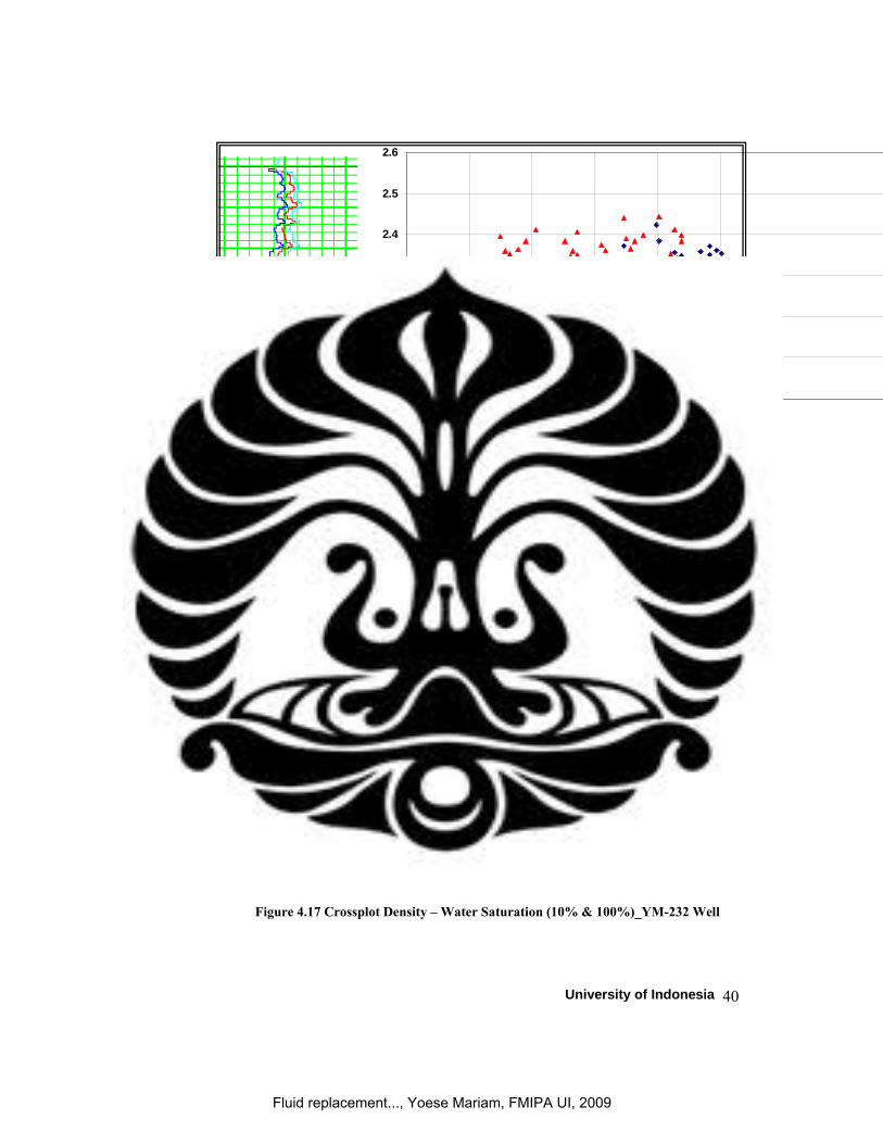
Figure 4.17 Crossplot Density – Water Saturation (10% &
100%)_YM-232 Well……………………………………
Figure 4.18 Crossplot Density – Water Saturation (40% & 70%)_YM-
232 Well………………………………………………….
Figure 4.19 Crossplot Velocity – Porosity (10% & 100% water
saturaton)_YM-232 Well………………………………….
Figure 4.20 Crossplot Density – Water Saturation (80% & 90%)_YM-
232 Well……………………………………
Figure 4.21 Crossplot Velocity – Porosity (40% & 70% water
saturaton)_YM-232 Well………………………………….
Figure 4.22 Crossplot P-impedance – Porosity YM-232 Well…………
Figure 4.23 Crossplot P-impedance – Water Saturation YM-232 Well..
Figure 4.24 Crossplot Velocity – Water Saturation (10% &
100%)_YM-247 Well……………………………………
Figure 4.25 Crossplot Velocity – Water Saturation (40% & 70%)_YM-
247 Well…………………………………………………..
Figure 4.26 Crossplot Density – Water Saturation (10% &
100%)_YM-247 Well……………………………………
Figure 4.27 Crossplot Density – Water Saturation (40% & 70%)_YM-
247 Well…………………………………………………...
Figure 4.28 Crossplot Velocity – Porosity (10% & 100% water
saturaton)_YM-247 Well………………………………….
Figure 4.29 Crossplot Velocity – Porosity (40% & 70% water
saturaton)_YM-247 Well………………………………….
Figure 4.30 Crossplot P-impedance – Porosity YM-247 Well…………
Figure 4.31 Crossplot P-impedance – Water Saturation YM-247 Well..
Figure 4.32 Synthetic Seismic at YM-232 Well with 2000 ft Offset
(Insitu Case & Saturated Case)……………………………
Figure 4.33 AVO Crossplot at YM-232 Well with 2000 ft Offset……..
Figure 4.34 Synthetic Seismic at YM-247 Well with 2000 ft Offset
(Insitu Case & Saturated Case)……………………………
Figure 4.35 AVO Crossplot at YM-247 Well with 2000 ft Offset……...
Figure 4.36 The Behavior of Sonic Transit Time in The Reservoir
40
41
42
43
44
44
45
47
48
49
50
51
52
52
53
53
54
54
55
Fluid replacement..., Yoese Mariam, FMIPA UI, 2009

ix
Rock as Fluid Content Increases. Red Indicates Oil & Blue
Indicates Water. (Suprajitno Munadi, 2007)………………
Figure 4.37 AVO Analysis (Intercept & Gradient of Top & Bottom
Telisa Sand) for Synthetic of YM-232 Well (insitu case &
substituted with 10%water saturation)…………………….
Figure 4.38 AVO Analysis (Intercept & Gradient of Top & Bottom
Telisa Sand) for Synthetic of YM-232 Well (substituted
with 70% & 100% water saturation)………………………
Figure 4.39 AVO Analysis (Intercept & Gradient of Top & Bottom
Telisa Sand) for Synthetic of YM-247 Well (insitu case &
substituted with 10% water saturation)……………………
Figure 4.40 AVO Analysis (Intercept & Gradient of Top & Bottom
Telisa Sand) for Synthetic of YM-247 Well (substituted
with 70% & 100% water saturation)………………………
Figure 4.41 The Correlation Coefficient Real Amplitude to Model after
Substituted Insitu Case YM-232 Well…………………
Figure 4.42 ρ, Vp, & Vs_Synthetic Offset Gathers (insitu case,
substituted with 10%, & 100% water saturation)_YM-232
Well………………………………………………………..
Figure 4.43 The Correlation Coefficient Real Amplitude to Model
after Substituted with 10% Water Saturation YM-232
Well………………………………………………………..
Figure 4.44 The Correlation Coefficient Real Amplitude to Model after
Substituted with 70% Water Saturation YM-232 Well……
Figure 4.45 ρ, Vp, & Vs_Synthetic Offset Gathers (insitu case,
substituted with 40%, & 70% water saturation)_YM-232
Well………………………………………………………..
Figure 4.46 The Correlation Coefficient Real Amplitude to Model after
Substituted with 90% Water Saturation YM-232 Well……
Figure 4.47 The Correlation Coefficient Real Amplitude to Model after
Substituted with 100% Water Saturation YM-232 Well…..
Figure 4.48 ρ, Vp, & Vs_Synthetic Offset Gathers (insitu case,
substituted with 80%, & 90% water saturation)_YM-232
56
56
57
57
58
59
59
60
60
61
61
62
Fluid replacement..., Yoese Mariam, FMIPA UI, 2009

x
Well………………………………………………………..
Figure 4.49 The Correlation Coefficient Real Amplitude to Model
Amplitude after Normalized YM-232 Well……………….
Figure 4.50 The Correlation Coefficient Real Amplitude to Model
Amplitude for Insitu Case YM-247 Well………………….
Figure 4.51 The Correlation Coefficient Amplitude Model to Real
Amplitude after Substituted with 10% Water Saturation
YM-247 Well……………………………………………..
Figure 4.52 The Correlation Coefficient Amplitude Model to Real
Amplitude after Substituted 40% Water Satruation YM-
247 Well…………………………………………………...
Figure 4.53 ρ, Vp, & Vs_Synthetic Offset Gathers (insitu case,
substituted with 10%, & 100% water saturation)_YM-247
Well………………………………………………………..
Figure 4.54 The Correlation Coefficient Amplitude Model to Real
Amplitude after Substituted with 70% Water Saturation….
Figure 4.55 ρ, Vp, & Vs_Synthetic Offset Gathers (insitu case,
substituted with 40%, & 70% water saturation)_YM-247
Well………………………………………………………..
Figure 4.56 The Correlation Coefficient Amplitude to Real Amplitude
after Substituted with 100% Water Satruation _ YM-247
Well………………………………………………………..
Figure 4.57 The Correlation Coefficient between Real Amplitude &
Model Amplitude after Normalized _ YM-247 Well……..
Figure 4.58 The Amplitude Distribution from Real Seismic………….
62
63
63
64
64
65
65
66
66
67
68
Fluid replacement..., Yoese Mariam, FMIPA UI, 2009

University of Indonesia iii
Abstract
Rock physics data is a tool for fluid identification and quantification in reservoir, and also plays an important part in any fluid substitution study that may provide a valuable tool for modeling various fluid scenarios. This thesis presents the results of the two well cases where the effect of rock and fluid properties on seismic response are illustrated. Both of wells (YM-232 and YM-247) show the effect of replacing hydrocarbons with brine. This effectt illustrates how rock and fluid properties along with reflection amplitudes can be used to estimate fluid type in YM field. First synthetic using the original case. And the other synthetic by using FRM case, with an assumption that the fluid was brine/oil and the mineralogy was clean sand. These amplitude was extracted to be correlated with the real seismic data. Finally, a good correlation was obtain from a model to estimate the fluid type in prospect based on amplitude information in seismic data. In other word, we can understand the effect of hydrocarbon saturation on synthetic offset gathers. This analysis can be use as one of parameter to improve seismic 3D interpretation and to reduce drilling risk.
Abstrak
Data Rock Physics adalah alat untuk identifikasi fluida, perhitungan dalam reservoar, dan bagian penting dalam studi substitusi fluida untuk memodelkan berbagai macam fluida. Thesis ini merupakan hasil dari penelitian dua sumur untuk melihat pengaruh dari batuan dan properti fluida terhadap respon seismik. Kedua sumur tersebut adalah (YM-232 dan YM-247) merupakan oil well yang menunjukkan pengaruh dari substitusi hidrokarbon dengan air. Akibat dari substitusi fluida terhadap batuan dan properti fluida menunjukkan respon tertentu pada refleksi amplitude, variasi amplitude tersebut dapat digunakan sebagai guide untuk memperkirakan penyebaran jenis fluida pada lapangan YM. Pertama dengan melakukan sintetik pada keadaan insitu. Diikuti dengan sintetik pada kondisi tersaturasi (FRM), dengan manganggap bahwa fluida adalah air/minyak dan mineral adalah batu pasir bersih. Amplitude ini akan diekstrak untuk dikorelasikan dengan data seismic yang sebenarnya. Koefisian korelasi yang memiliki nilai tinggi (~1) dijadikan sebagai model untuk memprediksi tipe fluida pada area prospek yang didasarkan pada informasi amplitude dari data seismik. Dengan kata lain, kita dapat memahami efek dari saturasi hidrokarbon terhadap synthetic offset gathers. Analisis ini digunakan sebagai salahsatu parameter untuk mengembangkan interpretasi data seismic 3D & untuk menekan/mengurangi resiko pengeboran.
Fluid replacement..., Yoese Mariam, FMIPA UI, 2009

University of Indonesia 1
Chapter 1
Introduction
1.1. Background
One of the productive reservoirs in South Sumatra Basin, is sandstones of
the Telisa formation. Now, reservoir pressure decreases, gas comes out of solution,
remaining oil phase changes, net stress increases, and rock stiffens. To maintain
the production rate, exploration efforts continue with new ideas and concepts. The
Telisa sandstone, consists of very fine to fine grained sandstones with minor
shales, deposited in a shallow marine shoreface setting during both sea level
lowstand and transgression.
Rock physics data allow us to make an analysis, which provides a tool for
fluid identification and quantification in reservoir, and also plays an important role
in any fluid substitution study that may provide a valuable tool for modeling
various fluid scenarios.
According to Castagna (2001), an objective of seismic analysis is to
quantitatively extract lithology, porosity, and pore fluid content directly from
seismic data. Rock physics provides the fundamental basis for seismic lithology
determination. The ultimate question in rock physics for direct hydrocarbon
indication is ‘How do velocities change when pore fluid content changes?’. More
specifically, we need a rock physics model that can transform velocities from one
saturation state to another.
A simple example combines Gassmann’s deterministic equation for fluid
substitution with statistics inferred from log, core, and seismic data to detect
hydrocarbons from observed seismic velocities. The formulation is applied to a
well log example for detecting the most likely pore fluid and quantifying the
associated uncertainty from observed sonic and density logs. The formulation
offers a convenient way to implement deterministic fluid substitution equations in
the realistic case when natural geologic variations cause the reference porosity and
velocity to span a range of values.
Fluid replacement..., Yoese Mariam, FMIPA UI, 2009

University of Indonesia 2
1.2. Objectives
The objectives of this thesis are :
1) To predict the elastic behaviour of rock property by the fluid replacement
methods.
2) To understand the effect of hydrocarbon saturation on synthetic offset gathers
3) To get a model as the best practice of quantitative and qualitative predictions,
the model is expected could be applied and tested to other exploration and/or
development field in South Sumatra.
1.3. Study Area
The study area is located in South Sumatra basin. The largest oil field in the
region is the YM oil field. It is believed that one of the potential candidates is
sandstone of the Telisa formation. Telisa sandstone contributes significant
additional reserves at YM field where production after hydraulic fracturing of 20
wells could reach 4,000 BOPD. While in Old YM, production of 7 wells (after
hydraulic fracturing) reached 750 BOPD.
The Telisa Sandstone, which includes the sandstones in the lower part of the
Telisa formation, consists of very fine to fine-grained sandstones with minor
shales, deposited in a shallow marine shoreface setting during both sea level
lowstand and transgression. The acoustic impedance contrast between the
sandstones and the overlying and underlying “Telisa” shales is very small because
of highly argillaceous content of the sandstone. The hydrocarbon potential in
this “Telisa” sandstone play remains unknown, but the results are encouraging.
Several successful tests have been conducted through the hydraulic fracturing
efforts. Although most of the sandstones are relatively tight, the reservoir flows oil.
Fluid replacement..., Yoese Mariam, FMIPA UI, 2009
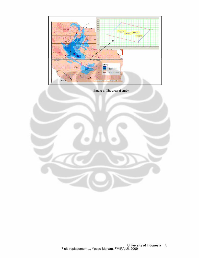
University of Indonesia 3
Figure 1. The area of study
YM-247YM-232
YM-242
YM-227
YM-247YM-232
YM-242
YM-227
Fluid replacement..., Yoese Mariam, FMIPA UI, 2009

University of Indonesia 4
Chapter 2
Theoretical Background
2.1 Regional Geology Setting
2.1.1 Structure & Tectonic
The study area is part of the YM Block, within South Sumatera Basin in
Palembang Province, Indonesia. The South Sumatra Basin was formed as a
result of crustal extension at Paleogene time. The basins is divided into three
sub-basins : Jambi sub-basin, Central Palembang sub-basin, and South
Palembang sub-basin. The dominant structure within the basin are : : WNW-
ESE, N-S, NW-SE and ± N 300E (Pulunggono et. al., 1992), which were
generated by both Australian Plate and Sundaland interaction.
The WNW-ESE strike slip system is the oldest structure generated during
tectonic compression phase in Pre-Tertiary time. The lithology of the basement
complexes consist of the Mesozoic igneous rock as wells as Paleozoic and
Mesozoic metamorphic and carbonate.
During early Tertiary time (Eocene to Oligocene), tectonic stress and
extension (resulting from northward movement of the Australian plate) formed
rift or half-graben complexes along much of southern margin of the Sunda
Shelf plate (Hall, 1997; Longley, 1997; Sudarmono, et. al., 1997). The half-
graben complexes were formed by N-S trend normal fault and reactivated
WNW-ESE growth fault. In this event, deposits began to fill the basin in
response to the half-graben architectural style and basin subsidence (Bishop,
1988). Additional synrift deposits of tuffaceous sands, conglomerates, breccias
and clays have deposited in fault and topographic low by alluvial, fluvial and
lacustrine processes. The sediments were deposited in a transgressive-
regressive cycles.
Many of the normal faults that formed the depositional basin in South
Sumatra have been reactivated and some have been reversed during Miocene to
Plio-Pleistocene compression and basin inversion (Sudarmono et. al., 1997).
Fluid replacement..., Yoese Mariam, FMIPA UI, 2009

University of Indonesia 5
The Plio-Pleistocene compression created the NW-SE trending, a normal
type fault with some lateral displacement as the most prominent feature, and
some other small faults and folds (Hutapea, 1998).
2.1.2 Tectonostratigraphy
The Lemat Formation has been deposited in a continental environment
during Paleocene to Early Oligocene time. This formation is normally bounded at
its base and top by an unconformity (Guruh et. al, 2003). The coarse clastic
member of the Lemat Formation is composed of sandstones, clays, rock fragment,
breccias, granite wash.
Sedimentation was renewed in the Upper Oligocene to Lower Miocene
with the deposition of the Talangakar marine clastic (TAF) during transgressive
cycle in deltaic to shallow marine environment.
Figure 2.1. Stratigraphy South Sumatera
Fluid replacement..., Yoese Mariam, FMIPA UI, 2009

University of Indonesia 6
Widespread marine transgression in the Late Oligocene to Early Miocene
resulted in clastic deposits overlying Talangakar Formation and in developments of
platform carbonates and carbonate build-up of the Baturaja Formation (BRF)
above the TAF.
Maximum transgression in the Middle Miocene deposited the clastic
shallow marine of the Gumai (Telisa) Formation across the region. It is
characteristically fossiliferous, marine shale, containing occasional thin beds of
glauconitic limestone.
Development of the Barisan Mt., and possible volcanic islands to the south
and southeast during Mid. Miocene – Plio Pleistocene, further decreased and then
cut off and overwhelmed marine influence and added new clastic and volcano
clastic sources from those directions (Hamilton, 1979).
The Formation which has been deposited during regressive cycle is
Airbenakat Formation and Muaraenim Formation. The Airbenakat Formation
composed of shale with glauconitic sandstones and occasional limestone, deposited
in a neritic environment at the base grading to a shallow marine environment at the
top. The Muaraenim Formation has been deposited in shallow marine-brackish (at
the base), paludal, deltaplain, and non-marine environment and are composed of
sandstones, mudstones and coal (Guruh et, al, 2003).
2.2 Telisa Sandstone Characterizations
The telisa sandstone is the lower part of The Gumai Formation which has
been deposited during Early Miocene (NN4-NN3; Geoservices, 2001). It is
bounded by Top BRF at the lower part.
The lithology of the telisa sand interval consists of shale, glauconitic
calcareous sandstone, calcareous sandstone and thin bed limestone. Interbedded
limestone and shale present in the lower part of the telisa sand interval. This
lithology shows coarsening upward and it can be recognized from the cores and log
character. It is overlaid by hummocky cross stratification calcareous sandstone.
The hummocky sandstone is overlaid by shale with thin intercalated fine sand.
The telisa Sandstone, which includes the sandstones in the lower part of the
Telisa formation, consists of very fine to fine grained sandstones with minor
Fluid replacement..., Yoese Mariam, FMIPA UI, 2009

University of Indonesia 7
shales, deposited in a shallow marine shoreface setting during both sea level
lowstand and transgression. The acoustic impedance contrast between the
sandstones and the overlying and underlying “telisa” shales is very small because
of highly argillaceous content of the sandstone.
The Telisa formation is lithostratigraphically defined as shallow to deep
open marine, dark grey shales. The shallow marine shales have been observed in
the Palembang High area. In this region, the lower part of the formation usually
contains thin reservoir sandstones called “Telisa Sandstone” and has thicknesses
ranging from 20 to 80 feet.
Wireline log motifs of the Telisa sandstone sequence varies significantly
from well to well. The sequence in the YM wells generally shows a blocky motif,
occasionally coarsening upward in the lower portion and fining upward in the
upper part, with an erosional surface in between. Based on this log shape and core
descriptions, the sandstones can be subdivided into several more detailed facies
lobes. In general, the sandstones are light olive gray, all fine and very fine grained,
clacerous, angular to subrounded, very well sorted lithic arenites with feldspar and
substantial numbers of globigerinids, small benthic foraminifers, small echinoid
spines, and splinters of vertebrate bone. It is a mix of sediment particles, created in
a fully marine environment (pelagic skeletal materials) with detrital particles (fine
sand and some clay mud) wafted in from the nearby coast. Wavy lamination and
ripple bedding, and bioturbated to various degrees, suggest deposition below the
fair weather wave base but it could be close to the storm wave base.
The overall Telisa sandstone sequence in the Palembang High region was
deposited during N5-N6 (middle Early Miocene). The water depth is increasing
from the top Baturaja to the shales overlying the Telisa sandstone : middle neritic
to upper bathyal. This is consistent with the major transgression period during
deposition of the Telisa formation. Following this transgression, a series of
regional regression occurred when the Palembang Group (Lower, Middle, and
Upper Palembang Formations) was deposited across the South Sumatra Basin.ma
The Telisa sandstone is present at shallow depths between 1700’ and 2500’.
The sandstone generally has low permeability causing low production. To improve
the production performance, the stimulation technique called “hydraulic
Fluid replacement..., Yoese Mariam, FMIPA UI, 2009

University of Indonesia 8
fracturing” has been employed. This technique uses hydraulic power to create
crack or opening at the reservoir, followed by pumping sand to fill the crack to
avoid closing.
Efforts to optimize the fracturing results have been made using six sigma
(statistical approach) and analytical approaches. The goal is to focus on increasing
oil gain from the fracturing job. The first step is to identify all factors that could
impact oil gain. The candidate selection criteria include area (field), resistivity, and
hydrocarbon pore thickness (HPT). Fracturing design includes fracturing length,
fracturing conductivity, propant size, and propant loads. Each of these factors is
evaluated using statistical analysis.
The second step is to evaluate data using a statistical approach: hypothesis
test, such as t-test and F-test. The t-test is to compare the mean of the two data sets
while the F-test is to compare the standard deviation of the two data sets. By using
these hypothesis tests the impact of the factors to the fracturing results can be
predicted. The evaluation continues for all of the factors and is combined with the
analytical approach using a fracturing simulator to determine the candidate
selection criteria and fracturing design.
The third step is the execution plan and field trials in the YM wells to
confirm the work results. The TSO fracturing design was applied in the Y Field
wells and the long hydraulic fracturing design was applied in the M wells.
The fourth step is monitoring work. Initially the oil production, after the
fracturing job, from the selected YM wells is high. There was significant oil gain
improvement after the work. The mean oil gain after the work was 220 BOPD (35
m3/day) compared to the mean oil gain before the work of 168 BOPD (26.7
m3/day). Standard deviation also decreased from 186 BOPD (26.9 m3/day) to 130
BOPD (20.7 m3/day). The performance of the wells will have to be closely
monitored.
There are some challenges in optimizing fracturing job results such as sand
flow back to the well bore, production drop after production for 3-5 months, and
high water cut. Sand flow back to the well bore will not only cause problems for
the facilities such as pipe line and pumps, but will also result in productivity
reduction. Both the causes of the problems and how to control them needs to be
addressed. The application of resin-coated sand may be one suitable means of
Fluid replacement..., Yoese Mariam, FMIPA UI, 2009

University of Indonesia 9
preventing this happening in the future. The production drop after initially good
production appears to happen in those wells that have extremely low permeability,
as indicated by the low resistivity values. To develop the wells that have resistivity
less than 5 ohm-m, will need further economic study will be required.
2.3 Rock Physics Theory
Rock physics reservoir characterization is based on applying rock physics
relations, such as between velocity and porosity, to a volume of seismic velocity or
impedance resulting from seismic inversion. The relevant rock physics laws are
often derived from well log data. The spatial scale of log measurements is much
smaller than the seismic scale. It is important to upscale rock physics relations used
or to make sure that they hold at the seismic scale.
Physical properties of porous rocks, such as seismic velocity, depend on
elastic properties of the porous frame and the pore-space filling material. The
elastic properties such as velocity, density, impedance, and Vp/Vs ratio take an
important role in reservoir characterization because they are related to the reservoir
properties. To analyze these elastic properties, rock physics knowledge is a bridge
that links the elastic properties to the reservoir properties such as water saturation,
porosity, and shale volume.
Rock physics is an indispensable tool for an efficient interpretation, providing
the basic relationship between the lithology, fluid, and geological deposition
environment of the reservoir. Also, rock physics modeling can be utilized to build
a template for efficient reservoir characterization (Φdegaard and Avseth, 2004;
Avseth et al., 2006; Andersen and Wijngaarden, 2007). In reservoir property
analysis, the lithology and fluid content or saturation can not be predicted
efficiently by identifying different clusters in the cross plot of elastic properties. In
contrast, the elastic properties inverted from seismic data can be efficiently
interpreted in conjunction with a rock physics template, which in turn can be used
to predict lithology and fluid content.
Gassmann’s equation is applied to estimate the fluid substitution effect in a
rock physics template and thereby the elastic modulus of dry and saturated rock.
Fluid replacement..., Yoese Mariam, FMIPA UI, 2009

University of Indonesia 10
The pore fluid properties are controlled by reservoir pressure, temperature, and
water saturation.
Usually, upon water saturation from the dry state, P-wave increases slightly and S-
wave decrease slightly. The velocity response to water saturation is rather complex
and physically controlled by the influence of the pore fluid on the rock moduli :
Compresional (P) velocity……………………………………………equation (2.1)
Shear (S) velocity……………………………………………………..equation (2.2)
First equation is the compresional (or P) velocity, which is the velocity for
the particle motion parallel to the direction of propagation. The second
equation is the shear (or S) velocity which is the velocity for the particle
motion perpendicular to the direction of propagation.
2.3.1. Rock Physics Properties of Shaly Sand
By analogy with the friable-sand model, we use the modified Hashin
Shtrikman lower bound to model constant-clay lines for shaly sands. These
lines can be used to define subfacies of sands where the facies changes
associated with varying clay content. Alternatively, we can use the more
empirical Vp-porosity-clay trends of Han (1986), or the lithology lines of
Vernik (1992).
Fluid replacement..., Yoese Mariam, FMIPA UI, 2009

University of Indonesia 11
In shaly sands, we can assume that the clay particles fill in the pores
between the sand grains. Assuming shaly sands to be uncemented, we can
apply the friable-sand model (i.e. Hertz-Mindlin plus modified lower bound
Hashin-Shtrikman) to calculate constant-clay content lines for friable shaly
sands. We obtain Kdry and µdry for the mixed lithology, and using
Gassmann’s equation we can calculate the corresponding water-saturated
moduli. The critical porosity will be lower for shaly sands than for sands (10-
40%), depending on the clay content. The higher the clay content, the lower the
critical porosity will be. The critical porosity will never reach zero since the
clay particles have internal porosity. The next input parameters to consider are
the mineral moduli. Since we are mixing quartz and clay particles, we need to
calculate effective mineral moduli, just like we did for the silty shales. The
mineral moduli represent the projections of the frame moduli, given by the
modified lower Hashin-Shtrikman bound, at zero porosity. The moduli
calculated from Voight or Reuss should be approximately the same for most
mineral mixtures. However, if we have very soft clays (e.g. smectite or illite)
Figure 2.2 Lines of Vp versus porosity for shales with varying silt content. The lines are modeled using modified lower bound Hashin-Shtrikman
combined with Hertz-Mindlin theory
Fluid replacement..., Yoese Mariam, FMIPA UI, 2009

University of Indonesia 12
mixed with relatively stiff quartz, the difference between the two methods can
be significant. We assume that the effective mineral moduli are given by the
Voight average equations, representing the stiffest possible alternative of the
mixed quartz-clay mineral :
Kmixed = (1-C)Kqz + CKclay
And
µmixed = (1-C)µqz + Cµclay
Voight average equations…………………………………………equation (2.3)
As an alternative to constant-clay content lines, we can also model increasing
clay content trends in the velocity-porosity plane. Marion (1990) introduced a
topological model for sand-shale mixtures to predict the interdependence
between velocity, porosity, and clay content. For shaly sands, it can be
assumed that clay particles are strictly located within the sand pore space.
Then, total porosity will decrease linearly with increasing clay content.
When clay content exceeds the sand porosity, the addition of clay will cause
the sand grains to become disconnected, as we go from grain-supported to clay-
supported sediments (i.e shales). The total porosity evolution of a sand-shale
mixture, as a function of increasing clay content.
Fluid replacement..., Yoese Mariam, FMIPA UI, 2009

University of Indonesia 13
Marion applied Gassmann’s equations to calculate the velocities of shaly sand. We
can use Gassmann to replace porous fluids with pore-filling clay (treating clay like
a liquid). When clay content is less than the sand porosity, clay particles are
assumed to be located within the pore space of the load-bearing sand. The clay
will stiffen the pore-filling material, without affecting the frame properties of the
sand. Therefore, increasing clay content will increase the stiffness and velocity of
the sand-shale mixture as the elastic moduli of the pore-filling material (fluid and
clay) increases.
Figure 2.3 Porosity and P-wave velocity versus clay content for shaly sands and sandy shales.
Note the porosity minimum and velocity maximum at the transition from grain-supported sediment to
clay-supported sediment. (Adapted from Marion, 1990)
Fluid replacement..., Yoese Mariam, FMIPA UI, 2009

University of Indonesia 14
2.4. Fluid Substitution – Gassmann
Prior to delving into Gassmann, we must first define and briefly discuss the
bulk and shear moduli of the rock, as well as the bulk modulus of the pore-
filling fluid.
2.4.1 Rock Properties
Gassmann’s equation relates the saturated bulk modulus of the rock (Ksat)
to its porous frame properties and the properties of the pore-filling fluid. The
bulk modulus, or incompressibility, of an isotropic rock is defined as the ratio
of hydrostatic stress to volumetric strain. Values for bulk modulus can be
obtained either by dynamic laboratory measurements of velocities or from
analysis of wireline log data (typical static measurements for the moduli violate
the assumption of infinitesimal strain, and should be avoided for fluid
substitution purposes). Whether from dynamic velocity measurements or from
wireline log data, we can relate the bulk modulus of a rock, Ksat, to its
compressional velocity, shear velocity, and bulk density.
2.4.2. Using Gassmann’s Equation
Before begin fluid substitution using equation , first must determine the
porosity of the rock, Ф, the properties of the fluids (Kfl, ρfl) that occupy the
pore space, the bulk modulus of the mineral matrix (Ko) , and the bulk
modulus of the porous rock frame (K*). All four components may be defined
or inferred through laboratory measurement or analysis of wireline log data.
Gassmann’s equation relates the bulk modulus of a rock to its pore, frame, and
fluid properties, as follows :
Gassmann Formula……………………………………………….equation (2.4)
Fluid replacement..., Yoese Mariam, FMIPA UI, 2009

University of Indonesia 15
2.4.3. Porosity
Porosity is routinely calculated from core data or from analysis of wireline
log data is rewritten and solved for porosity. Because logging tools do not
directly measure porosity or bulk density, calibration of the log-derived
porosity to measured core porosity is highly desirable, and in some
instances(e.g., when dealing with complex lithologies or low porosity rocks)
may significantly alter the results of a fluid substitution. Core calibration may
also be particularly important if the formation is invaded by drilling fluids.
2.4.5 Fluid Properties
Prior to performing a fluid substitution, three approaches are commonly
used for determining the bulk modulus and density of the in-situ pore-filling
fluid, as well as those of the new fluid to be model :
1) the properties are measured directly (at reservoir temperatures and
pressures) from pore fluids recovered from the reservoir
2) the properties are calculated from equations of state (see McCain, 1990;
Danesh, 1998)
3) the properties are calculated from an empirical calculator (e.g., Batzle and
Wang, 1992)
Generally, the difference between the two is small unless the fluid has a
relatively high gas-oil-ratio (GOR).
Because there typically are two or more fluid phases occupying the pore
space of a reservoir rock, we must calculate a bulk modulus and density of the
individual fluid end members, and then mix the fluids according to the
following physica; rules. Gassmann’e equation assumes all the pore space is
connected and pore pressure is equilibrated throughout the rock.
2.4.6 Matrix Properties
To calculate the bulk modulus of the mineral matrix, Ko, information on
the composition of the rock must be available. If core samples are available,
mineral abundance may be determined using conventional laboratory
techniques. In the absence of core data, lithology can be approximated from
wireline logs by simple clay volume (Vclay) analysis and assuming the two
Fluid replacement..., Yoese Mariam, FMIPA UI, 2009

University of Indonesia 16
mineral end members are quartz and clay. For more complex lithologies,
however, other techniques must be applied which allow the volumetric
abundance of the mineral constituents to be estimated.
2.4.7 Frame Properties
Prior to applying Gassmann’s equation, it is necessary to determine the
bulk modulus of the porous rock frame, K*. This is the low-frequency, drained
bulk modulus of the rock. Once determined, K* is held constant during the
course of a fluid substitution. Note that the shear modulus, G, is also a frame
property of the rock and is therefore also held constant during the typical fluid
substitution process.
2.4.8 Calculating Velocities
Assume we have calculated porosity (ф) along with the matrix and frame
properties of the rock (Ko, K*, and G). This allows us to calculate a new
saturated bulk modulus for any desired fluid.
2.4.9 Dry Frame Bulk Modulus, K*
Application of Gassmann’s equation is dependent upon accurate
determination of the porous frame properties of the rock (K* and G). In order
Table 2. Bulk modulus, shear modulus, and bulk density Of common rock forming minerals.* Values are from
Carmichael (1989).
Fluid replacement..., Yoese Mariam, FMIPA UI, 2009

University of Indonesia 17
to calculate the shear modulus, G, it is only necessary to know the bulk density
and shear velocity of the information.
2.5 Effect of fluid saturation on seismic properties
The seismic response of reservoirs is directly controlled by compressional
(P-wave) and shear (S-wave) velocities Vp and Vs respectively along with
densities.
Clearly, bulk modulus is more sensitive to water saturation. The bulk-
volume change and causes a pressure increase in pore fluid (water). This
pressure increase stiffens the rock frame and causes an increase in bulk
modulus. Shear deformation, however, does not produce a pore-volume
change, and consequently different fluids do not affect shear modulus.
Therefore, any fluid-saturation effect should correlate mainly to a change in
bulk modulus.
Numerous assumptions are involved in the derivation and application of
Gassmann’s equation :
1. the porous material is isotropic, elastic, monomineralic, and homogenous;
2. the pore space is well connected and in pressure equilibrium (zero-
frequency limit);
3. the medium is a closed syste with no pore-fluid movement across
boundaries;
4. there is no chemical interaction between fluids and rock frame (shear
modulus remains constant)
2.6 Theoretical Models
The theoretical models are primarily continue mechanics approximations of
the elastic, viscoelatic, or poroelastic properties of rocks. Among the most
famous are the poroelastic models of Biot (1956), who was among the first to
formulate the coupled mechanical behavior of a porous rock embedded with a
linear viscous fluid. The Biot equations reduce to the famous Gassmann (1951)
relations at zero frequency; hence, we often refer to “Biot-Gassmann” fluid
substitution. Biot (1962) generalized his formulation to include a viscoelastic
frame, which was later pursued by Stoll and Bryan (1970). The “squirt model”
Fluid replacement..., Yoese Mariam, FMIPA UI, 2009

University of Indonesia 18
of Mavko and Nur (1975) and Mavko and Jizba (1991) quantified a grain-scale
fluid interaction, which contributed to the frame viscoelasticity. Dvorkin and
Nur (1993) explicity combined Biot and squirt mechanisms in their “Bisq”
model.
2.6.1 Internal Consistency and Saturation Modeling
Fluid substitution models should always be carefully evaluated for quality
and internal consistency. For instance, when oil or gas is substituted into a
brine sand, bulk densities should always decrease and shear velocities should
always increase.
To aid as a quality-control check on fluid substitutions and in order to best
understand how velocities and densities should vary for any given sand, it is
often instructive to generate saturation models, where Gassmann’s
relationships are used to calculate Vp, Vs, and ρB as a function of water
saturation. These types of models are particularly important for understanding
the rare case when compressional velocities for a gas sand are faster than those
for oil in the same sand. This situation can occur when the bulk density
decreases at a faster rate than the saturated bulk modulus as gas saturation is
increased.
Fluid substitution is an important part of seismic attribute work, because it
provides the interpreter with a tool for modeling and quantifying the various
fluid scenarios. The most commonly used technique for doing this involves the
application of Gassmann’s equations.
The objective of fluid substitution is to model the seismic properties
(seismic velocities) and density of a reservoir at a given reservoir condition
(e.g., pressure, temperature, porosity, mineral type, and water salinity) and pore
fluid saturation such as 100% water saturation or hydrocarbon with only oil or
only gas saturation.
Modeling the changes from one fluid type to another requires that the
effects of the starting fluid first be removed prior to modeling the new fluid,
and the moduli (bulk and shear) and bulk density of the porous frame are
calculated. Once the porous frame properties are properly determined, the rock
Fluid replacement..., Yoese Mariam, FMIPA UI, 2009

University of Indonesia 19
is saturated with the new pore-fluid, and the new effective bulk modulus and
density are calculated.
Gassmann fluid substitution can be performed by begin with an initial
set of velocities and densities, Vp, Vs, and ρ corresponding to the rock with an
initial set of fluids, which we call “fluid I”. These velocities often come from
well logs, but might also be the result of an inversion or theoretical model.
The most common scenario is to begin with an initial set of velocities
and densities, Vp, Vs, and ρ corresponding to the rock with an initial set of
fluids, which we call “fluid 1”. These velocities often come from well logs, but
might also be the result of an inversion or theoretical model.
When calculating fluid substitution, it is obviously critical to use
appropriate fluid properties. To our knowledge, the Batzle and Wang (1992)
empirical formulas are the state of the art.
The density and bulk modulus of most reservoir fluids increase as pore
pressure increases.
The density and bulk modulus of most reservoir fluids decrease as
temeperature increases.
The Batzle-Wang formulas describe the empirical dependences of gas, oil,
and brine properties on temperature, pressure, and composition.
The Batzle-Wang bulk moduli are the adiabatic moduli, which we believe
are appropriate for wave propagation.
In contrast, standart PVT data are isothermal. Isothermal moduli can be ~
20% too low for oil, and a factor of 2 too low for gas. For brine, the two do
not differ much.
Fluid replacement..., Yoese Mariam, FMIPA UI, 2009

University of Indonesia 20
Chapter 3
Data & Methodology
.
3.1. Methodology
Methodology used to achieve the goals of this study includes the main
activities such as : selection and data validation, data processing and quality
control (QC data), data processing and analysis. In principle, a series of major
activities (work flow) in this study can be simplified as follows:
Phase 1 involves the selection zone or interval Telisa formation which is the target
/ goal of this study. The selection is done based on the consideration of
completeness of data, scientific (geophysics, geology) and the expected results.
Phase 2 includes work-related clasification the systematics raw data, download
data, processes and tools help hardness and soft according with each type of data.
Conversion work, corrections, and rarefaction (smoothing) of data is done in this
phase 2.
Phase 3 will consist of the following jobs:
Computation, classification, and statistical data processing elastic properties and
rock physical variables that other studies that are relevant to this. Of the output
form of the various cross-plot, histogram, image, graphic and model. Relationships
rock properties and ductile developed by previous researchers tested against the
data set of research areas.
Phase 4 consists of the following work:
1. Develop and propose relationships quantitative and reasonable (reliable)
between properties resilient, physical, and texture based on zone stratigaphy rock
known in both these wells.
2. Comparing the results, the above results with previous studies of lithology
similar to lithology of Telisa formation and compares with theory and models that
have been universally accepted and that has been proposed by researchers in the
latest other areas (models, between others:)
Fluid replacement..., Yoese Mariam, FMIPA UI, 2009

University of Indonesia 21
3. Discuss and investigate in detail the differences between the results of this study
with the expected or with models and formulas that have been there. Propose
alternative solutions and models as a result of these differences.
4. Workflow studies documenting the physical and rock properties of Telisa
formation which may be applied to the formation of equivalent that there is oil in
the field.
3.1.1 Fluid Substitution
Fluid substitution performed on two wells in the area of research focused
on the Telisa sand, the reservoir (sandstone) is filled by fluid hydrocarbons that
contain oil.
Fluid Substitution is carried out to investigate the changes of fluid
saturation and its effect to Vp and Vs log in the presence of fluid of this reservoir.
Fluid Substitution analysis was performed in YM#232 & YM#247 wells, based on
the following data :
1. Gas gravity (gr/cc)
2. Oil gravity (gr/cc)
3. Formation pressure (reservoir) (psi)
4. Formation temperature (reservoir) (deg F)
5. Water salinity (ppm)
6. Gas Oil Ratio
This data can be obtained from the results of laboratory analysis of samples
taken from welltest reports.
The data obtained are:
1. Formation Temperature (reservoir) : 284 deg F
2. Formation Pressure (reservoir) : 1100 psi
3. Salinity : 4000 ppm
4. Oil gravity : 35.2 API
5. Gas gravity : 0.8929
6. Gas Oil Ratio (GOR) : 296 SCF/STB
Input data required in this analysis is the fluid substitution velocity (Vp and
Vs), or slowness, density, porosity, saturation of water (water saturation). Matrix
Fluid replacement..., Yoese Mariam, FMIPA UI, 2009

University of Indonesia 22
properties must also be used as input in the analysis this fluid substitution. For this
study, quartz mineral is used as a default.
Based on the calculation of average Gassmann, fluid substitution can be made
crossplot, with the assumption that the pore bulk modulus and dry rock poisson's
ratio fixed (the same) although porosity changed rock.
3.2 Data
Main data used in this study is the result of measurement data in the field
(raw data), in the form of data recording wells (Wireline log data) from four wells
(YM-227, 232, 242 & 247) that consist of gamma ray, density, neutron, resistivity,
SP, cali, and sonic (Vp & Vs).
Supporting data used in this study was results of the processing and interpretation
of data from the two well cases (YM-232 & 247), which consist of:
a. Petrophysical Analysis & Interpretation
b. Seismic data (post stack)
c. PVT data
d. Mudlog report
e. Report from Telisa Formation Study
3.3 Wavelet Extraction & Well Seismic Tie
The form of seismic signals (wavelet) influence the successfull of the
benchmarking process models between the trace and data trace. This is because of
the RC’s precission anyway, but if the signal will result in a form and amplitude
trace its model. Therefore, the signal that contain in the seismic waves can be
extracted correctly. This process is called wavelet extraction.
There are 2 methods for extracting seismic signals (Prastianto, 1991):
1. Signal extraction from wells without information
In circumstances such as this, that the presumption applied RC truly random
(random) so that the multiplication both of spectrum signal amplitude is the same
as the multiplication both of amplitude seismic trace, as a result of this self-
correlation spectrum of seismic trace, so that finally, to the conclusion that the
spectrum amplitude signal proportional to the spectrum amplitude of the seismic
Fluid replacement..., Yoese Mariam, FMIPA UI, 2009

University of Indonesia 23
trace. From the amplitude spectrum of this signal can do with gained by reverse
fourier transform.
2. Signal extraction wells with available data
In this case there are density and velocity data in the wells, so the AI can be
calculated well. AI from this well revealed in the RC pit. RC in the wells is
transformed first to the frequency area and the results are used to divide the
spectrum of seismic trace through wells. To get the form of signals, the Fourier
back tranformation made from the results of this spectrum.
Wavelet extraction stage is the very success of the inverse set. Extraction is
done with the wavelet method using the statistical seismic data only. The first stage
of the extraction is conducted to analyze the spectrum amplitudo from seismic data
and well log data and then taken the average. After that calculation is done on time
and phase shift of the initial wavelet (wavelet amplitude spectrum) to produce an
optimum correlation. Final stages of the wavelet extraction is the combination of
spectrum amplitude with phase shift and time, so the best wavelet which has the
highest price correlation between the synthetic seismogram.
The process of seismic well tie is a process to get the fitness reflektivity
between the well data and seismic data. The first step that is done, apply the
checkshot will the correct relationship between time and depth of the data well and
or seismic. Then proceed with the wavelet to extract synthetic seismogram can be
made that will dikorelasikan dnegan seismic data. Wavelet can be extracted from
seismic data, log data and the accuracy synthetic specified price from the high
correlation.
Fluid replacement..., Yoese Mariam, FMIPA UI, 2009

University of Indonesia 24
Figure 3. Work Flowchart
PetrophysicalAnalysis
Fluid Substitution
Synthetic
Sensitivity Analysis
Well Selection
Vp, Vs, ρ, ΦPVT Data
Vp, Vs, ρ (substituted with : 10%, 40%, 70%,
80%, 90%, & 100% water saturation)
Seismic Data
Calibrated Model Amplitude
PetrophysicalAnalysis
Fluid Substitution
Synthetic
Sensitivity Analysis
Well Selection
Vp, Vs, ρ, ΦPVT Data
Vp, Vs, ρ (substituted with : 10%, 40%, 70%,
80%, 90%, & 100% water saturation)
Seismic Data
Calibrated Model Amplitude
Fluid replacement..., Yoese Mariam, FMIPA UI, 2009

University of Indonesia
25
CHAPTER 4
Analysis & Interpretation
4.1. Data Processing
Processing data in this thesis has been done using the software Hampson
Russel (HRS) because the data used are logs and seismic data. The steps of data
processing which is done here consists of :
1. The petrophysical data from petrophysicist
2. Inputting data into software
3. Sensitivity analysis of rock properties by performing the calculation
from YM-227, YM-232, YM-242, YM-247 wells as a data base and
making some crossplot such as:
1. VpVs_Ratio vs Gamma Ray with color key Gamma Ray
2. VpVs_Ratio vs Gamma Ray with color key Saturation
3. VpVs_Ratio vs Gamma Ray with color key Porosity
Only log data (figure 4.1 & 4.2) from YM-232 (with reservoir zone at
2322 – 2377 ft MD) and YM-247 (the reservoir zone at 2810 – 2873 ft MD) wells
that will further analyze in this thesis.
Figure 4.1 Composite Log YM-232 Well
Fluid replacement..., Yoese Mariam, FMIPA UI, 2009

University of Indonesia
26
4.2. Sensitivity Analysis
Sensitivity analysis has been conducted to explore the parameters that have
a good correlation between petrophysics and seismic data. This parameter should
be seen on the scale of seismic resolution. By using the well log data we can
determine the type of reservoir rock, thickness of hydrocarbons zone (pay zone),
type of fluid in the reservoir and petrophysical parameters such as porosity,
saturation and others. The next crossplot was made by combining the well data to
seismic data to determine the petrophysical parameters which correlates well with
the seismic data.
The curve which are displayed has been selected only that related to thesis.
This is to investigate the relationship between petrophysical parameters and sonic
log. The cross plot has been limited only within the reservoir zone of the Telisa
formation.
Figure 4.2 Composite Log YM-247 Well
Fluid replacement..., Yoese Mariam, FMIPA UI, 2009

University of Indonesia
27
Figure 4.4 Porosity vs Sw & Porosity vs Vclay at YM-247 Well
Figure 4.3 Porosity vs Sw & Porosity vs Vclay at YM-232 Well
Porosity vs Sw & Clay Content
0
0.2
0.4
0.6
0.8
1
1.2
0 0.05 0.1 0.15 0.2 0.25 0.3
Porosity
Sw &
Cla
y C
onte
nt
Pore-SwPore-Vclay
Sw-Vclay-Pore
0
0.2
0.4
0.6
0.8
1
1.2
0.05 0.1 0.15 0.2 0.25 0.3 0.35
Porosity
Sw &
Cla
y C
onte
nt
Pore-SwPore-Clay
Fluid replacement..., Yoese Mariam, FMIPA UI, 2009

University of Indonesia
28
The trend of petrophysical properties from YM-232 and YM-247 wells is that if
the porosity increases, the saturation decreases (figure 4.3 & 4.4)
The crossplot was made from YM-227, YM-232, YM-242, and YM-247
wells as a data base. At the time Gamma Ray below 78 API within the yellow area
as sandstone, while above 78 API within the green area as shale. Gamma Ray 78
API as a cut off to differentiate the lithology, while VpVs_Ratio at 2.7 as a cut off
to distinguish pay and wet zone (figure 4.5, 4.6, & 4.7).
Figure 4.5 Crossplot (YM-227, 232, 242, & 247 Wells) Gamma Ray vs VpVs_Ratio with Color Key Gamma Ray
Sandstone
Shale
Fluid replacement..., Yoese Mariam, FMIPA UI, 2009

University of Indonesia
29
Those figure 4.6 & 4.7, there’s good correlation between porosity & saturation.
The fourth well is sensitive to these parameter. Its can separate the pay zone and
wet zone. The same trend can be seen at those crossplot.
4.3. Fluid Substitution
Shaly sands can be valuable reservoirs, so geophysical modeling of such
sands, including fluid substitution, is useful. The model concentrates on seismic
properties, i.e. density and velocity.
With the theory of fluid substitution proposed by Gassmann, we can predict
the changes of seismic response by changing fluid which is done using oil with
water. Theoretical calculations was performed by changing fluid saturation, and
correlating with nature petrophysics in seismic response.
Figure 4.6 Crossplot (YM-227, 232, 242, & 247 Wells) Gamma Ray vs VpVs_Ratio with Color Key Porosity
Shale
Sandstone
Fluid replacement..., Yoese Mariam, FMIPA UI, 2009

University of Indonesia
30
By changing the fluid saturation (with Sw 10%, 40%, 70%, 80%, 90% and
100%), the Vp and density log will change. This Vp log together with density log
can be used to construct the reflection coefficient. By convolving the reflection
coefficient with the extracted wavelet from seismic trace, we get the FRM
seismogram. FRM seismogram, this means that we know the synthetic which
contains fluid. The FRM seismogram can be used to investigate the fluid content
information in the field or real seismogram (seismic trace).
Fluid Substitution has been performed in two wells in the area of study and
focused in the reservoir zone “Telisa Sand”, the reservoir (sandstone) is filled by
oil.
Fluid Substitution is carried out to investigate the changes of fluid saturation and
its effect to density, Vp and Vs log in the presence of fluid of this reservoir.
Figure 4.7 Crossplot (YM-227, 232, 242, & 247 Wells) Gamma Ray vs VpVs_Ratio with Color Key Saturation
Shale
Sandstone
Fluid replacement..., Yoese Mariam, FMIPA UI, 2009

University of Indonesia
31
Fluid Substitution analysis was performed inYM-232 & YM-247 wells, based on
the following data (table 4.1) :
Input data needed in this analysis is the fluid substitution velocity (Vp and Vs) or
slowness (DTA & DTSF/DTXX), density, porosity, saturation of water (water
saturation). Matrix properties must also be used as input in the analysis of this
fluid.substitution For this thesis, quartz mineral is used as a default.
To process for calculating of the above formula, can be executed using
FRM module from HRS and the results can be seen in the logs above. Based on the
picture above, it can be explained that for the reservoir “Telisa Sand” with the
actual form of hydrocarbons in oil YM -232 & YM-247 wells, the changes of Sw
value is more sensitive to the increases of Vp or in other words that Vp increases
when it was completely oil saturated (figure 4.8 & 4.9).
The original saturation at YM-232 well is about 50% to 80%. It is substituted with
water saturation 10%, 40%, 70%, 80%, 90%, & 100%. When it was completely oil
saturated density decreases and Vp increases, while Vs increases. On the contrary,
it was completely water saturated density increases and Vp decreases. While Vs is
constant.
Table 4.1 Reservoir Properties
Property Value
Formation Temp. 284 deg F
Formation Pres. 1100 psi
Salinity 4000 ppm
Oil Gravity 35.2 API
Gas Gravity 0.8929
GOR 296 SCF/STB
Fluid replacement..., Yoese Mariam, FMIPA UI, 2009

University of Indonesia
32
YM-247 well has the saturation 50% to 80 %. The 10%, 40%, 70%, & 100% water
saturation were applied for the substitution. The density decreases while Vp
increases when it was completely oil saturated, and Vs is constant. On the contrary,
the density increases, Vp decreases, and Vs is constant when it was completely
water saturated.
4.4 Wavelet Extraction & Well Seismic Tie
Wavelet extraction process can be done using several methods. Firstly, we
should find out the frequency dominant which is 40 Hz in this case. From the
calculation, the tuning thickness is 62 ft and the reservoir thickness is 40 – 60 ft.
However, the objective is above seismic resolution.
Figure 4.8 Fluid Substitution at YM-232 Well (Substitution with Sw 10%, 70%, 90%, & 100%)
Fluid replacement..., Yoese Mariam, FMIPA UI, 2009

University of Indonesia
33
In this research on wavelet extraction is done with several methods,
including statistical methods (using the seismic data), using the data well, a
combination of extraction from seismic data and wells and to wavelet Ricker and
wavelet bandpass.
From several methods, we choose to use the wavelet obtained from Ricker. This
wavelet extraction process is done repeateadly (try and error), with the fox-value
wavelength and long taper to obtain the wavelet phase spectrum and the best.
Finally wavelet extraction on YM-232 & YM-247 wells applied Ricker 40 Hz, and
the correlation each well is 0.698 for YM-232 well and 0.635 at YM-247 well
(figure 4.11 & 4.12).
Figure 4.9 Fluid Substitution at YM-247 Well (Substitution with Sw 10%, 40%, 70%, & 100%)
Fluid replacement..., Yoese Mariam, FMIPA UI, 2009

University of Indonesia
34
Figure 4.11 Correlation with Ricker 40 Hz at YM-232 Well
Figure 4.10 Frequency Dominant is 40 Hz & Wavelet Extraction
Fluid replacement..., Yoese Mariam, FMIPA UI, 2009

University of Indonesia
35
4.5. Rock Physics Analysis & Synthetic Offset Gathers
Rock physics is an indispensable tool for an efficient interpretation,
providing the basic relationship between the lithology, fluid, and geological
deposition environment of the reservoir. The elastic properties such as velocity,
density, impedance, and Vp/Vs ratio take an important role in reservoir
characterization because they are related to the reservoir properties such as water
saturation, porosity, and shale volume.
This is the results of two well cases (YM-232 & YM-247) where the effects
of rock and fluid properties on seismic are illustrated. This case is an example from
YM field that shows the effect of hydrocarbons saturation on synthetic offset
gathers. This well contains a hydrocarbon from about 2322 to 2377 ft at YM-232
well and 2810 ft to 2873 ft at YM-247 well. From the logs (GR-Density-
Pwave_Swave), are able to construct a four layer model for the pay zone and its
over-and under-lying horizons. The layers are shale, sandstone as reservoir, shale,
and limestone. In other words, the reservoir is in between shale section.
Figure 4.12 Correlation with Ricker 40 Hz at YM-247 Well
Fluid replacement..., Yoese Mariam, FMIPA UI, 2009

University of Indonesia
36
4.5.1 The Analysis of The Telisa Sand Reservoir at YM-232 Well
Petrophysical analysis on YM-232 well in the Telisa Sand reservoir shows
the porosity is 20% – 27%. Gamma Ray reading at this resrevoir is high enough,
shows 60 - 80 API. The reservoir is very fine to fine sandstone with streak of shale.
The fluid contain in this reservoir is oil. Although the mudlog shows that high gas
readings (720 units). Pressure data in this well was achieved from MDT (Modular
Dynamic Tester).
The next rock properties analysis is P-impedance to perform calculations on the
density and sonic logs. The range P-imp in the Telisa Sand reservoir is 12,200 to
18,500 gr / cc * ft / sec.
Then, the analysis of rock properties is VpVs_Ratio. This analysis involves
the shear wave data recorded through the sonic log, called a shear DT (DTSF). The
value of VpVs_Ratio in the Telisa Sand reservoir is 1.3 – 2.25. This value is
correlate with the decrease of P-imp in this reservoir (figure 4.22 & 4.23).
From the figure that the P-imp value for insitu case, it is about 17000 ft/s*g/cc.
Actually, when it was substituted with 100% water saturation, the AI is very high,
it is about 19000 to 21000 ft/s*g/cc. And when it was completely oil saturated the
AI is about 13000 to 17000 ft/s*g/cc. We used the porosity as a constant value (the
original value).
Fluid replacement..., Yoese Mariam, FMIPA UI, 2009

University of Indonesia
37
Velocity vs Sw
2000
3000
4000
5000
6000
7000
8000
9000
10000
0.5 0.55 0.6 0.65 0.7 0.75 0.8 0.85 0.9 0.95 1
Sw
Velo
city
InsituInsitu10%_10%_
Figure 4.13 Crossplot Velocity – Water Saturation (10%) _YM-232 Well
2000
3000
4000
5000
6000
7000
8000
9000
10000
0.5 0.55 0.6 0.65 0.7 0.75
Fluid replacement..., Yoese Mariam, FMIPA UI, 2009

University of Indonesia
38
Velocity vs Sw
2000
3000
4000
5000
6000
7000
8000
9000
10000
0.5 0.55 0.6 0.65 0.7 0.75 0.8 0.85 0.9 0.95 1
Sw
Velo
city
Insitu_VsInsitu_Vp100%_Vs100%_Vp
Figure 4.14 Crossplot Veloctiy – Water Saturation (100%)_YM-232 Well
2000
3000
4000
5000
6000
7000
8000
9000
10000
0.5 0.55 0.6 0.65 0.7 0.75
Fluid replacement..., Yoese Mariam, FMIPA UI, 2009

University of Indonesia
39
Velocity vs Sw
2000
3000
4000
5000
6000
7000
8000
9000
10000
0.5 0.55 0.6 0.65 0.7 0.75 0.8 0.85 0.9 0.95 1
Sw
Velo
city
Insitu_VsInsitu_Vp40%_Vs40%_Vp70%_Vs70%_Vp
Velocity vs Sw
2000
3000
4000
5000
6000
7000
8000
9000
10000
0.5 0.55 0.6 0.65 0.7 0.75 0.8 0.85 0.9 0.95 1
Sw
Velo
city
Insitu_VsInsitu_Vp80%_Vs80%_Vp90%_Vs90%_Vp
Figure 4.15 Crossplot Velocity – Water Saturation (40% & 70%) YM-232 Well
Figure 4.16 Crossplot Velocity – Water Saturation (80% & 90%)_YM-232 Well
Fluid replacement..., Yoese Mariam, FMIPA UI, 2009
University of Indonesia
40
Density vs Sw
2
2.1
2.2
2.3
2.4
2.5
2.6
0.5 0.55 0.6 0.65 0.7 0.75 0.8 0.85 0.9 0.95 1
Sw
Den
sity Insitu
10%100%
Figure 4.17 Crossplot Density – Water Saturation (10% & 100%)_YM-232 Well
2
2.1
2.2
2.3
2.4
2.5
2.6
0.5 0.55 0.6 0.65 0.7 0.75
Fluid replacement..., Yoese Mariam, FMIPA UI, 2009

University of Indonesia
41
From YM-247 well, the range P-imp is about 18000 to 21000 ft/s*g/cc for
the original case. And also when it was completely oil saturated. But when it was
substituted with 100% water satruation, the P-imp increases, the value is 22000 to
24000 ft/s8g/cc. And the porosity that we used from the original case (constant).
To observe the changes of the fluid density (oil) and Vp to the actual the changes
of water saturation at YM-232 well, we will use fluid substitution by Gassmann.
The result indicates that the changes in density and vp fluida in the Telisa Sand
reservoir in this well is responsive to the gradually changing of 10%, 40%, 70%,
80%, 90% and 100% water saturation.
Analysis that is done is to create some crossplot of rock properties that have been
achieved from the previous analysis.
Density vs Sw
2
2.1
2.2
2.3
2.4
2.5
2.6
0.5 0.55 0.6 0.65 0.7 0.75 0.8 0.85 0.9 0.95 1
Sw
Den
sity Insitu
40%70%
Figure 4.18 Crossplot Density – Water Saturation (40% & 70%) YM-232 Well
Fluid replacement..., Yoese Mariam, FMIPA UI, 2009

University of Indonesia
42
Velocity vs Porosity
2000
3000
4000
5000
6000
7000
8000
9000
10000
0 0.05 0.1 0.15 0.2 0.25 0.3
Porosity
Velo
city
Insitu_VsInsitu_Vp10%_Vs10%_Vp100%_Vs100%_Vp
Figure 4. 19 Crossplot Velocity – Porosity (10% & 100% water saturation) YM-232 Well
0.1 0.15 0.2 0.25
Fluid replacement..., Yoese Mariam, FMIPA UI, 2009

University of Indonesia
43
Density vs Sw
2
2.1
2.2
2.3
2.4
2.5
2.6
0.5 0.55 0.6 0.65 0.7 0.75 0.8 0.85 0.9 0.95 1
Sw
Den
sity Insitu
80%90%
Figure 4.20 Crossplot Density – Water Saturation (80% & 90%) YM-232 Well
2
2.1
2.2
2.3
2.4
2.5
2.6
0.5 0.55 0.6 0.65 0.7 0.75
Fluid replacement..., Yoese Mariam, FMIPA UI, 2009

University of Indonesia
44
Figure 4.22 Crossplot P-impedance – Water Saturation YM-232 Well
P-imp - Sw
10000
12000
14000
16000
18000
20000
22000
24000
0.5 0.55 0.6 0.65 0.7 0.75 0.8 0.85 0.9 0.95 1
Sw
P-im
p
Insitu10%40%70%80%90%100%
Sw 100%
Figure 4.21Crossplot Velocity – Porosity (40% & 70% water saturation) YM-232 Well
Velocity vs Porosity
2000
3000
4000
5000
6000
7000
8000
9000
10000
0 0.05 0.1 0.15 0.2 0.25 0.3
Porosity
Velo
city
Insitu_VsInsitu_Vp40%_Vs40%_Vp70%_Vs70%_Vp
Fluid replacement..., Yoese Mariam, FMIPA UI, 2009

University of Indonesia
45
Then performed the same synthetic seismic routine and the results are
shown. Synthetic Offset Gathers made with the various variations offsets, 4500,
4000, 3500, 3000, 2500 and 2000 ft until resolved the pay zone. Actually, the
strong response can only be seen when it was completely oil or water saturated.
Compared to the insitu case, can be seen that the offset response is very similar,
however the reflection amplitudes increases that it was completely water saturated.
On the contrary, the reflection amplitudes decrease that assumed 10% water
saturation and clean sand.
Next, computed new Vp, Vs, and density values for the pay zone assuming that it
was completely water saturated. The synthetic seismic (figure 4.32 & 4.34) shows
a major change in character at all offsets. The polarity of the reflections are
completely reversed indicating that the hydrocarbons are a major factor only in this
model (at YM-232 well).
Figure 4.23 Crossplot P-impedance – Porosity YM-232 Well
P-imp - Pore
0
5000
10000
15000
20000
25000
0 0.05 0.1 0.15 0.2 0.25 0.3
Pore
P-im
pInsitu10%40%70%80%90%100%
Sw 100%
Fluid replacement..., Yoese Mariam, FMIPA UI, 2009

University of Indonesia
46
4.5.2 The Analysis of The Telisa Sand Reservoir at YM-247 Well
The porosity of Telisa Sand reservoir at YM-247 well is 20% to 30%,
based on petrophysical analysis. The reservoir quality is relatively good than Telisa
Sand reservoir at YM-232 well. The Gamma Ray log is 40 – 55 API. The mudlog
indicates that the lithology in this reservoir is fine to medium grain, while the gas
readings is 32 to 35 units. No MDT data in this well.
The P-imp in this reservoir is 18500 – 22000 gr/cc*ft/sec. This value is
higher than P-imp at the same reservoir with oil content at YM-232 well (figure
4.17). The VpVs_Ratio is 2.25 to 2.75, this value is higher than YM-232 well.
And this fenomena is related to the physics of fluid (oil) is quite low (35.2 API)
and the reservoir rock itself.
This well contains a hydrocarbon (oil) from about 2810 to 2873 ft. Next by
assuming that the fluid was brine and the mineralogy was clean sand (figure ). And
from fluid substitution analysis we can see the increases of water saturation (10%,
40%, 70%, 100%) affects the changing of Vp (fluid) that it was sensitive.
The Vp, Vs, and density from fluid substitution analysis will be applied on
seismic amplitude or called its as Synthetic Offset Gathers. It is made with various
variations offsets 4500, 4000, 3500, 3000 and 2000 ft. This analysis will compare
to insitu case. This figure shows taht the near offset response is very similar. When
computed new Vp, Vs, and density values for the pay zone assuming that it was
completely water saturated. The synthetic seismic shows a major change in
character at all offsets (figure 4.32 & 4.35).
Fluid replacement..., Yoese Mariam, FMIPA UI, 2009

University of Indonesia
47
Velocity vs Sw
2000
4000
6000
8000
10000
12000
14000
16000
0.4 0.5 0.6 0.7 0.8 0.9 1
Sw
Velo
city
Insitu_VsInsitu_Vp10%_Vs10%_Vp100%_Vs100%_Vp
Figure 4.24 Crossplot Velocity – Water Saturation (10% & 100%)_YM-247 Well
0.6 0.7 0.8
Fluid replacement..., Yoese Mariam, FMIPA UI, 2009

University of Indonesia
48
Velocity vs Sw
2000
4000
6000
8000
10000
12000
14000
16000
0.4 0.5 0.6 0.7 0.8 0.9 1
Sw
Velo
city
Insitu_VsInsitu_Vp40%_Vs40%_Vp70%_Vs70%_Vp
Figure 4.25 Crossplot Velocity – Water Saturation (40% & 70%)_YM-247 Well
Fluid replacement..., Yoese Mariam, FMIPA UI, 2009

University of Indonesia
49
Density vs Sw
1.7
1.8
1.9
2
2.1
2.2
2.3
2.4
2.5
2.6
2.7
0.4 0.5 0.6 0.7 0.8 0.9 1
Sw
Den
sity Insitu
10%100%
Figure 4.26 Crossplot Density – Water Saturation (10% & 100%)_YM-247 Well
0.6 0.7 0.8
Fluid replacement..., Yoese Mariam, FMIPA UI, 2009

University of Indonesia
50
Density vs Sw
1.7
1.8
1.9
2
2.1
2.2
2.3
2.4
2.5
2.6
2.7
0.4 0.5 0.6 0.7 0.8 0.9 1
Sw
Den
sity Insitu
40%70%
Figure 4.27 Crossplot Desnity – Water Saturation (40% & 70%)_YM-247 Well
0.6 0.7 0.8
Fluid replacement..., Yoese Mariam, FMIPA UI, 2009

University of Indonesia
51
Velocity vs Porosity
2000
4000
6000
8000
10000
12000
14000
0 0.05 0.1 0.15 0.2 0.25 0.3 0.35 0.4
Porosity
Velo
city
Insitu_VsInsitu_Vp10%_Vs10%_Vp100%_Vs100%_Vp
Figure 4.28 Crossplot Velocity – Porosity (10% & 100% water saturation)_YM-247 Well
0.15 0.2 0.25 0.3
Fluid replacement..., Yoese Mariam, FMIPA UI, 2009

University of Indonesia
52
Figure 4.30 Crossplot P-impedance - Porosity YM-247 Well
Velocity vs Porosity
2000
4000
6000
8000
10000
12000
14000
0 0.05 0.1 0.15 0.2 0.25 0.3 0.35 0.4
Porosity
Velo
city
Insitu_VsInsitu_Vp40%_Vs40%_Vp70%_Vs70%_Vp
Figure 4.29 Crossplot Velocity – Porosity (40% & 70% water saturation)_YM-247 Well
P-imp - Porosity
10000
12000
14000
16000
18000
20000
22000
24000
26000
0.05 0.1 0.15 0.2 0.25 0.3 0.35
Porosity
P-im
p
Insitu10%40%70%100%
Fluid replacement..., Yoese Mariam, FMIPA UI, 2009

University of Indonesia
53
Figure 4.32 Synthetic Seismic at YM-232 Well with offset 2000 ft (insitu case, after substituted with 10%, 40%, 70%, 80%, 90%, & 100% water saturation)
Figure 4.31 Crossplot P-impedance – Water Saturation YM-247 Well
P-imp - Sw
10000
12000
14000
16000
18000
20000
22000
24000
26000
0.5 0.55 0.6 0.65 0.7 0.75 0.8 0.85 0.9 0.95 1
Sw
P-im
p
Insitu10%40%70%100%
Fluid replacement..., Yoese Mariam, FMIPA UI, 2009

University of Indonesia
54
Figure 4.34 Synthetic Seismic at YM-247 Well with offset 2000 ft (insitu case, after substituted with 10%, 40%, 70%, & 100% water saturation)
Figure 4.33 AVO Crossplot at YM-232 Well with offset 2000 ft (insitu case, after substituted with 10%, 40%, 70%, 80%, 90%, & 100% water saturation)
Amplitude vs Offset
-0.4
-0.3
-0.2
-0.1
0
0.1
0.2
0 500 1000 1500 2000 2500
Offset
Am
plitu
de
InsituSw10%Sw70%Sw80%Sw90%Sw100%40%
Fluid replacement..., Yoese Mariam, FMIPA UI, 2009

University of Indonesia
55
Synthetic seismic from YM-232 & YM-247 wells show a major change of
amplitude response (substituted with 10% & 100% water saturation) in character at
all offsets, indicating that the hydrocarbons are a major factor in this model, as
opposed to simply changes in lithology.
We assumed that the amplitude response close related to sonic wave propagation
(DT). The oil content affects the sonic wave propagation (DT), in a specific
manner: at low interval oil content, the sonic transit time decreases gradually &
drops suddenly at a specific value, above this value the sonic transit time seems
does not change with the increase of oil content. The water content affects the
sonic wave propagation in a specific interval of water saturation (figure 4.36).
And the second assumption, that, the pore space (porosity Φ) is filled with a fluid
of density ρfl & bulk modulus Kfl. In other words, the bulk modulus of saturated
rock equals the bulk modulus of the skeleton plus a term which depends on the
fluid.
Figure 4.35 AVO Crossplot at YM-247 Well with offset 2000 ft (insitu case, after substituted with 10%, 40%, 70%, & 100% water saturation)
Amplitude vs Offset
0
0.02
0.04
0.06
0.08
0.1
0.12
0.14
0 500 1000 1500 2000 2500
Offset
Am
plitu
de
Insitu10%40%70%100%
Fluid replacement..., Yoese Mariam, FMIPA UI, 2009

University of Indonesia
56
Figure 4.36 The Behavior of Sonic Transit Time in The Reservoir Rock
as Fluid Content Increases. Red Indicates Oil & Blue Indicates Water.
(Suprajitno Munadi, 2007)
Figure 4.37 AVO Analysis (Intercept & Gradient of Top & Bottom Telisa Sand)
for Synthetic of YM-232 Well
(insitu case & substituted with 10% water saturation)
Fluid replacement..., Yoese Mariam, FMIPA UI, 2009

University of Indonesia
57
Figure 4.38 AVO Analysis (Intercept & Gradient of Top & Bottom Telisa Sand)
for Synthetic of YM-232 Well
(substituted with 70% & 100% water saturation)
Figure 4.39 AVO Analysis (Intercept & Gradient of Top & Bottom Telisa Sand)
for Synthetic of YM-247 Well
(insitu case & substituted with 10% water saturation)
Fluid replacement..., Yoese Mariam, FMIPA UI, 2009

University of Indonesia
58
Figure 4.40 AVO Analysis (Intercept & Gradient of Top & Bottom Telisa Sand)
for Synthetic of YM-247 Well
(substituted with 70% & 100% water saturation)
From YM-232 well at figure 4.33, 4.37 & 4.38 can be interpreted that the
synthetic after substituted with 10% & 70% water saturation, it can be classified as
near-zero impedance contrast sands. Same as the above classification, the synthetic
after substituted with 100% water saturation is near-zero impedance contrast sands,
but it looks like polarity change.
While, YM-247 from figure 4.35, 439 & 4.30 is interpreted as high impedance
sand.
4.8 Comparison between Model Amplitude and Real Seismic
A problem often encountered in exploration and development geophysics is
to estimate the fluid type in prospect based on amplitude information in seismic
data. The method applied data on sand velocity, density, porosity, clay content and
expected fluid types as input into the rock physics software for estimation of
acoustic impedance and reflectivity for various types of hydrocarbon saturation.
And the result is the coefficient from the model have good correlation with the real
seismic, at YM-247 well.
Fluid replacement..., Yoese Mariam, FMIPA UI, 2009

University of Indonesia
59
Each of correlation coefficient from YM-232 well : when it was completely water
saturated is 0.12, 0.87 for the original saturation, when it was substituted with 70%
and 90% water saturation : 0.87 and 0.88 , and for 10% water saturation is 0.86.
While the smallest correlation is found at YM-232 well, when it was completely
water saturated.
Figure 4.41 The Correlation Coefficient between Real Amplitude & Model Amplitude at Insitu Case (original Sw) _YM-232 Well
Amp(Real Seismic) vs Amp(Orig Sw)
-0.2-0.15-0.1
-0.050
0.050.1
0.150.2
0.250.3
0 2 4 6 8 10 12 14
Actual
Mod
el R=0.87
Figure 4.42 ρ, Vp, & Vs _ Synthetic Offset Gathers (insitu case, substituted with 10% & 100% water saturation) _YM-232 Well
Fluid replacement..., Yoese Mariam, FMIPA UI, 2009

University of Indonesia
60
Figure 4.44 The Correlation Coefficient between Real Amplitude & Model Amplitude After Substituted with 70% Water Saturation _ YM-232 Well
Figure 4.43 The Correlation Coefficient between Real Amplitude & Model Amplitude After Substituted with 10% Water Saturation _ YM-232 Well
Amp(Real Seismic) vs Amp(Sw10%)
-0.2
-0.1
0
0.1
0.2
0.3
0 2 4 6 8 10 12 14
Actual
Mod
el
Amp(Real Seismic) vs Amp(Sw70%)
-0.2-0.15-0.1
-0.050
0.050.1
0.150.2
0.25
0 2 4 6 8 10 12 14
Actual
Mod
elR=0.86
R=0.87
Fluid replacement..., Yoese Mariam, FMIPA UI, 2009

University of Indonesia
61
Figure 4.46 The Correlation Coefficient between Real Amplitude & Model Amplitude After Substituted with 90% Water Saturation _ YM-232 Well
Amp(Real Seismic) vs Amp(Sw90%)
-0.2-0.15-0.1
-0.050
0.050.1
0.150.2
0.25
0 2 4 6 8 10 12 14
Actual
Mod
el
R=0.88
Figure 4.45 ρ, Vp, & Vs _ Synthetic Offset Gathers (insitu case, substituted with 40% & 70% water saturation) _YM-232 Well
Fluid replacement..., Yoese Mariam, FMIPA UI, 2009

University of Indonesia
62
Overall, model amplitude YM-232 well, close to the real seismic data, except for
100% water saturation. However, good correlation is achieved when it was
substituted by water saturation.
After the model was normalized to seismic data, then, its can be applied to predict
the fluid in other area within the field.
Figure 4.47 The Correlation Coefficient between Real Amplitude & Model Amplitude After Substituted with 100% Water Saturation _ YM-232 Well
Amp(Real Seismic) vs Amp(Sw100%)
-0.06-0.04-0.02
00.020.040.06
0.080.1
0 2 4 6 8 10 12 14
Actual
Mod
el R=0.12
Figure 4.48 ρ, Vp, & Vs _ Synthetic Offset Gathers (insitu case, substituted with 80% & 90% water saturation) _YM-232 Well
Fluid replacement..., Yoese Mariam, FMIPA UI, 2009

University of Indonesia
63
Figure 4.49 The Correlation Coefficient between Real Amplitude & Model Amplitude After Normalized _ YM-232 Well
R=0.77
Amp(Real Seismic) vs Amp(Orig Sw)
-0.2-0.15-0.1
-0.050
0.050.1
0.150.2
-20 -15 -10 -5 0 5 10 15
Actual
Mod
el
Figure 4.50 The Correlation Coefficient between Real Amplitude & Model Amplitude for Insitu Case _ YM-247 Well
R=0.90
Norm Model
-5
-3
-1
1
3
5
7
9
1 3 5 7 9 11 13
Real Seismic
Mod
el
Fluid replacement..., Yoese Mariam, FMIPA UI, 2009

University of Indonesia
64
Amp(Real Seismic) vs Amp(Sw10%)
-0.2-0.15-0.1
-0.050
0.050.1
0.150.2
-20 -15 -10 -5 0 5 10 15
Actual
Mod
elR=0.80
Figure 4.51 The Correlation Coefficient between Real Amplitude & Model Amplitude After Substituted with 10% Water Saturation _ YM-247 Well
Amp(Real Seismic) vs Amp(Sw40%)
-0.2-0.15-0.1
-0.050
0.050.1
0.150.2
-20 -15 -10 -5 0 5 10 15
Actual
Mod
el
Figure 4. 52 The Correlation Coefficient between Real Amplitude & Model Amplitude After Substituted with 40% Water Saturation _ YM-247 Well
R=0.84
Fluid replacement..., Yoese Mariam, FMIPA UI, 2009

University of Indonesia
65
Amp(Real Seismic) vs Amp(Sw70%)
-0.2-0.15-0.1
-0.050
0.050.1
0.150.2
-20 -15 -10 -5 0 5 10 15
Actual
Mod
el
R=0.87
Figure 4.54 The Correlation Coefficient between Real Amplitude & Model Amplitude After Substituted with 70% Water Saturation _ YM-247 Well
Figure 4. 53 ρ, Vp, & Vs _ Synthetic Offset Gathers (insitu case, substituted with10% & 100% water saturation) _YM-247 Well
Fluid replacement..., Yoese Mariam, FMIPA UI, 2009

University of Indonesia
66
Amp(Real Seismic) vs Amp(Sw100%)
-0.25-0.2
-0.15
-0.1-0.05
00.05
0.10.15
-20 -15 -10 -5 0 5 10 15
Actual
Mod
el
Figure 4.56 The Correlation Coefficient between Real Amplitude & Model Amplitude After Substituted with 100% Water Saturation _ YM-247 Well
R=0.98
Figure 4.55 ρ, Vp, & Vs _ Synthetic Offset Gathers (insitu case, substituted with 40% & 70% water saturation) _YM-247 Well
Fluid replacement..., Yoese Mariam, FMIPA UI, 2009

University of Indonesia
67
Also with YM-232 well, YM-247 model can be applied to predict the fluid in other
area within the field. A good correlation is achieved when it was substituted by
100% water saturation, 0.98. And the second is when it was substituted by 70%
water saturation, 0.87.
This is summary of correlation amplitude model with real seismic data from YM-
247 well (table 4.2 & 4.3) :
Norm Model
-15
-10
-5
0
5
10
15
-15 -10 -5 0 5 10 15
Real Seismic
Mod
el
R=0.96
Figure 4. 57 The Correlation Coefficient between Real Amplitude & Model Amplitude After Normalized _ YM-247 Well
The Correlation Coefficient Amplitude Model with Real Seismic (YM-232 well)
Original Case 0.8754
Substituted with Sw 10% 0.8656
Substituted with Sw 70% 0.8793
Substituted with Sw 90% 0.8842
Substituted with Sw 100% 0.1244
Norm Model 0.7745
Table 4.2 The Correlation Coefficient Model Amplitude to Real Seismic (YM-232 Well)
Fluid replacement..., Yoese Mariam, FMIPA UI, 2009

University of Indonesia
68
The range of model amplitude is -0.2 to 0.24. While the amplitude distribution
from real seismic is -10 to 10 (figure 4.45). The amplitude model will be calibrated
and correlated to real seismic, to achieve the correlation coefficient. Then, those
model (normalization model) ready to be applied within field (figure 4.44 & 4.52).
The Correlation Coefficient Amplitude Model with Real Seismic(YM-247 well)
Original Case 0.9028
Substituted with Sw 10% 0.808
Substituted with Sw 40% 0.8449
Substituted with Sw 70% 0.8756
Substituted with Sw 100% 0.9894
Norm Model 0.9691
Tabl 4.3 The Correlation Coefficient Model Amplitude to Real Seismic (YM-247 Well)
Figure 4.58 The Amplitude Distribution from Real Seismic
Fluid replacement..., Yoese Mariam, FMIPA UI, 2009

University of Indonesia 69
CHAPTER 5
Conclusions and Recommendation
The original reservoir sand interval (YM-232 & YM-247 wells) (oil filled)
shows high porosity, low Vclay, high water saturation, decreasing P-imp. Gassmann’s
equation provide the seismic interpreter with a powerful framework for evaluating
various fluid scenarios which might give rise to an observed seismic. When applied
fluid substitution at YM-232 & YM-247 wells, the changing of Vp is sensitive to the
increases of water saturation. At the time completely oil saturated, the porosity
increases and P-imp decreases. When, it was completely water saturated, P-imp
increases and also porosity.
The Synthetic Offset Gathers is a way to understand the effect of hydrocarbon
saturation on synthetic offset gather. From YM-232 and YM-247 wells, the offset
response is very similar, however the reflection amplitudes increases that it was
completely water saturated. These two examples illustrate that quantitative
interpretation of fluid type can be made based on computed rock properties and
seismic data. They also show the importance of fluid properties and reflections
amplitudes. These amplitudes applied as a model and will be calibrated and correlated
to the real seismic. The good correlation coefficient is considered to be closed to the
real seismic data. And this model can be applied to predict the fluid in other area
within the field.
YM-232 & YM-247 wells have good correlation, when it was substituted with
90% & 70% water saturation, the correlation coefficient are 0.88 and 0.87 . However,
at YM-247 well, a good correlation is achieved when it was substituted with 100% &
70% water saturation, are 0.98 and 0.87. Actually, by knowing those model or we
called as normalization model (after normalized to real seismic) : 0.77 (YM-232 well)
and 0.96 (YM-247 well) can be applied within field as parameter to improve when
interpreted 3D seismic data. Model amplitude of YM-232 & YM-247 wells, each of
which can be a model that represents each field. Of course, after doing some test of
Fluid replacement..., Yoese Mariam, FMIPA UI, 2009

University of Indonesia 70
some well of each Y & M field. At YM-247 well, a model represents Y field, have the
characters on the density log is contrast, so the rock more dominant than fluid.
This improved interpretation can reduce drilling risk and ultimately increase asset
value by avoiding wet zone in this case.
The sensitivity analysis to critical reservoir parameters, has been done. Its
worked at YM Field. Gassmann formula can be applied in this field, as we can see that
the rock bulk modulus will change if the fluid changes, but the rock shear modulus
will not. The advance analysis like relations between Vp and Vs are key to the
determination of lithology from seismic or sonic log data, as well as for direct seismic
identification of pore fluids using, for example, AVO analysis is needed. And seismic
inversion to see the lateral distribution of reservoir properties. In this thesis, I’ve not
made AVO, because of unavailability of gathers data.
Fluid replacement..., Yoese Mariam, FMIPA UI, 2009

Universitas Indonesia 71
REFERENCES
Avseth P, Mukerji T., & Mavko G., 2005. Quantitative Seismic Interpretation,
Applying Rock Physics Tools to Reduce Interpretation Risk. Cambridge University Press. UK
Chaveste, Alvaro., May 2003. Risk reduction in estimation of petrophysical
properties from seismic data through well-log modeling, seismic modeling, and rock properties estimation. Core Laboratories Reservoir Technolgoies Division, Houston, Texas, U.S.
Kumar, Dhananjay., January 4, 2006. A Tutorial on Gassmann Fluid Substitution :
Formulation, Algoritmn and Matlab Code. Chevron Energy Technology Company, California
Mavko, Gary. Introduction to Rock Physics. Stanford Rock Physics Laboratory. Munadi, Suprajitno., October, 2007. The Effect of Oil Content on Sonic Wave
Propagation (Analyses from Well Log Data). Lemigas Contributions Vol. 30 No. 2
Munadi, Suprajitno, 2000. Aspek Fisis Seismologi Eksplorasi. Program Studi
Geofisika, Jurusan Fisika, FMIPA, Universitas Indonesia, Depok. Pennington, W.D., 2008. Advanced Seismic Petrophysics. NEXT Course Note.
Bandung M. Smith*, Tad., H. Sondergeld, Carl., S. Rai, Candra, March-April 2003. Tutorial
Gassmann Fluid Substitutions : A tutorial. Geophysical, Vol. 68, No. 2. R.M.I. Argakoesoemah., Rahardja Maria., Winardhi Sonny., Tarigan Rudhy.,
Febriwan Tino., Aimar Amritzar, Agustus 30-September 1, 2005. Telisa Shallow Marine Sandstone as An Emerging Exploration Target in Palembang High, South Sumatra Basin. 30th Annual Convention & Exhibition, IPA
D. Walls, Joel. Fluids, AVO, and Seismic Amplitudes : field examples. PetroSoft
Inc. Walls, Joel., Dvorkin Jack., Carr, Matt., 2004. Well Logs and Rock Physics in
Seismic Reservoir Characterization. Rock Solid Images. Houston, Texas, U.S.A
Fluid replacement..., Yoese Mariam, FMIPA UI, 2009