fluid mechanics - tufts university kinds of forces are typically considered in the study of fluid...

FLUID MECHANICS Based on CHEM_ENG 421 at Northwestern University

NEWTON’S LAWS | 1

TABLE OF CONTENTS 1 Newton’s Laws ....................................................................................................................... 3

1.1 Inertial Frames .............................................................................................................................. 3 1.2 Newton’s Laws ............................................................................................................................. 3 1.3 Galilean Invariance ....................................................................................................................... 3

2 Mathematical Description of Fluid Flow ............................................................................. 4 2.1 Fields and Forces .......................................................................................................................... 4 2.2 Continuity Equation ...................................................................................................................... 4 2.3 The Stress Tensor .......................................................................................................................... 4 2.4 Newton’s Law of Viscosity........................................................................................................... 6 2.5 Generalized Gauss’ Theorem ........................................................................................................ 6 2.6 Newton’s Equation of Motion for a Fluid ..................................................................................... 7 2.7 Navier-Stokes Equation ................................................................................................................ 8 2.8 Simplifying the Navier-Stokes Equation ...................................................................................... 9

2.8.1 Reduced Pressure ..................................................................................................................................... 9 2.8.2 Reynolds Number .................................................................................................................................... 9 2.8.3 Approximate Solutions of the Navier-Stokes Equation ........................................................................... 9

3 Forces and Torques: Sphere in Stokes Flow ..................................................................... 11 3.1.1 Problem Setup ........................................................................................................................................ 11 3.1.2 Force Due to Tangential Stress .............................................................................................................. 11 3.1.3 Force Due to Viscous Normal Stress ..................................................................................................... 13 3.1.4 Force Due to Pressure ............................................................................................................................ 14 3.1.5 Total Force on the Sphere from the Fluid .............................................................................................. 15

4 One-Dimensional Flow in Viscous Fluids .......................................................................... 16 4.1 Poiseuille Flow ............................................................................................................................ 16 4.2 Stokes Flow around a Sphere: Trial Solutions ............................................................................ 17 4.3 Plate Suddenly Set in Motion: Time-Dependent Flow ............................................................... 20

5 Vorticity ................................................................................................................................ 23 5.1 Definition of Vorticity ................................................................................................................ 23 5.2 Curl of Navier-Stokes ................................................................................................................. 23 5.3 Low Reynolds Number ............................................................................................................... 23 5.4 High Reynolds Number .............................................................................................................. 24 5.5 Circulation ................................................................................................................................... 25

6 Boundary Layer Theory ..................................................................................................... 27 6.1 High Reynolds Number Flow over a Flat Plate Parallel to Flow ................................................ 27 6.2 Low Reynolds Number Flow over a Flat Plate (any direction) .................................................. 28 6.3 High Reynolds Number Flow over a Flat Plate Perpendicular to Flow ...................................... 29

7 Appendix: Vector Calculus ................................................................................................. 30 7.1 Coordinate Systems .................................................................................................................... 30

7.1.1 Cartesian Coordinate System ................................................................................................................. 30 7.1.2 Cylindrical Coordinate System .............................................................................................................. 30 7.1.3 Spherical Coordinate System ................................................................................................................. 31 7.1.4 Surface Differentials .............................................................................................................................. 31 7.1.5 Volume Differentials ............................................................................................................................. 31

7.2 Mathematical Operations ............................................................................................................ 32 7.2.1 Magnitude .............................................................................................................................................. 32 7.2.2 Dot Product ............................................................................................................................................ 32 7.2.3 Cross Product ......................................................................................................................................... 32

7.3 Operators ..................................................................................................................................... 32 7.3.1 Gradient ................................................................................................................................................. 32 7.3.2 Divergence ............................................................................................................................................. 33

NEWTON’S LAWS | 2

7.3.3 Curl ........................................................................................................................................................ 33 7.3.4 Laplacian ............................................................................................................................................... 34

7.4 Common Identities of Second Derivatives ................................................................................. 34 7.5 Surface Integration ...................................................................................................................... 34

7.5.1 The Surface Integral............................................................................................................................... 34 7.5.2 Divergence Theorem.............................................................................................................................. 35

7.6 Stokes’ Theorem ......................................................................................................................... 35 8 Appendix: Practical Problem Solving Methods................................................................ 36

8.1 Deriving Expressions for Velocity, Pressure, and Stress ............................................................ 36 8.2 Common Boundary Conditions .................................................................................................. 36 8.3 Using Newton’s Law of Viscosity .............................................................................................. 36 8.4 Calculating Mean Velocity and Flow Rate ................................................................................. 37

9 Appendix: Tabulated Expressions ..................................................................................... 38 9.1 Expressions for Newton’s Law of Viscosity ............................................................................... 38

9.1.1 Cartesian Coordinates ............................................................................................................................ 38 9.1.2 Cylindrical Coordinates ......................................................................................................................... 38 9.1.3 Spherical Coordinates ............................................................................................................................ 38

9.2 Expressions for the Continuity Equation .................................................................................... 38 9.2.1 Cartesian Coordinates ............................................................................................................................ 38 9.2.2 Cylindrical Coordinates ......................................................................................................................... 39 9.2.3 Spherical Coordinates ............................................................................................................................ 39

9.3 Expressions for the Navier-Stokes Equation............................................................................... 39 9.3.1 Cartesian Coordinates ............................................................................................................................ 39 9.3.2 Cylindrical Coordinates ......................................................................................................................... 39 9.3.3 Spherical Coordinates ............................................................................................................................ 39

NEWTON’S LAWS | 3

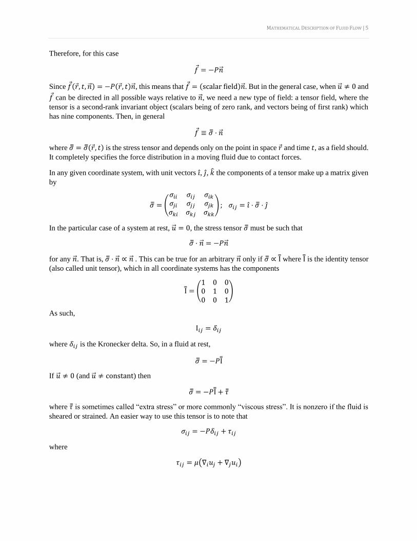
1 NEWTON’S LAWS 1.1 INERTIAL FRAMES Newton’s first law states that velocity, �⃗�, is a constant if the force, �⃗�, is zero. Newton’s second law is the

very famous �⃗� = 𝑚�⃗�. At first glance, it would seem that Newton’s first law is simply a recapitulation of

the second law. After all, since acceleration, �⃗�, is simply the first time derivative of velocity, then if velocity

is constant, acceleration is zero and thereby force is zero. However, there is indeed a reason to explicitly

state Newton’s first law. Newton’s first law sets the frame of reference as the inertial frame. Examples of

nearly inertial frames are the Earth, an Earth-bound lab, and a train moving with constant speed with respect

to the Earth.

Any rapidly rotating frame is a non-inertial reference frame. Non-inertial but accelerating frames rely on

Einstein’s equivalence principle, which states that

“All the phenomena in a frame that are accelerating with respect to an inertial frame with

acceleration �⃗�𝑓 happens as if in an inertial frame with apparent gravity, where the acceleration of

gravity is given by −�⃗�𝑓.”

1.2 NEWTON’S LAWS In more exact terms, the first law can be said to mean:

“There exists a frame of reference such that in this frame a body not acted upon by any force continues

to be either in the state of rest or a uniform motion (i.e. with constant velocity). Such a frame is called

inertial. Any frame moving with constant velocity with respect to an inertial frame is also inertial.”

This should make sense and establishes a context for Newton’s second law. Newton’s second law can be

effectively worded as “In an inertial frame, a body of mass 𝑚 acted upon by a force �⃗�, acquires an

acceleration �⃗� = �⃗�/𝑚.”

1.3 GALILEAN INVARIANCE The last sentence of Newton’s first law in the prior subsection is a little more nuanced than it appears. Let’s

prove that for any frame moving with uniform motion with respect to an inertial frame is also inertial. This

is frequently called the Galilean invariance.

Consider two inertial frames given by 𝑆 and 𝑆′ that both share a universal time. Suppose 𝑆′ is in relative

uniform motion to 𝑆 with speed 𝑣. Therefore, for a position 𝑟′(𝑡) in 𝑆′ frame and position 𝑟(𝑡) in 𝑆 frame

then

𝑟′(𝑡) = 𝑟(𝑡) + 𝑣𝑡

The velocity of the object in the 𝑆′ frame is given by

𝑢′(𝑡) =𝑑𝑟′(𝑡)

𝑑𝑡=𝑑(𝑟(𝑡) + 𝑣𝑡)

𝑑𝑡=𝑑𝑟(𝑡)

𝑑𝑡+ 𝑣 = 𝑢(𝑡) + 𝑣

Differentiating once more to yield acceleration gets

𝑎′(𝑡) =𝑑𝑢′(𝑡)

𝑑𝑡=𝑑(𝑢(𝑡) + 𝑣)

𝑑𝑡=𝑑𝑢(𝑡)

𝑑𝑡= 𝑎(𝑡)

Therefore, assuming the mass is identical in both inertial frames, Newton’s laws in frame 𝑆 should also be

true in frame 𝑆′ (and all other frames move with uniform relative motion to 𝑆).

MATHEMATICAL DESCRIPTION OF FLUID FLOW | 4

2 MATHEMATICAL DESCRIPTION OF FLUID FLOW 2.1 FIELDS AND FORCES Fluids can be described based on velocity vector fields, �⃗⃗�(𝑟, 𝑡), and pressure scalar fields 𝑃(𝑟, 𝑡). These

variables satisfy differential equations, which express the two basic laws of nature: the conservation of mass

and Newton’s second law. The conservation of mass states that fluid can move from point to point, but it

cannot be created or destroyed. Newton’s second law implies that we use an inertial frame of reference;

otherwise, fictitious forces such as centrifugal and Coriolos forces must be included.

Two kinds of forces are typically considered in the study of fluid mechanics. The first is long-range “body

forces” such as gravity, usually known per unit mass (�⃗�) or per unit volume (e.g. 𝜌�⃗�). The second is surface

“contact forces” due to the short-range action of fluids on fluids (or solids) across an imaginary (or real)

interface, such as pressure or viscous friction.

2.2 CONTINUITY EQUATION The conservation of mass for a fluid, and by extension the continuity equation, will be derived below.

1. Let’s assume an arbitrary control volume in space, given by 𝑉. It has a surface 𝑆 and a normal

direction given by �⃗⃗�.

2. Since mass is conserved, we can say that

(total rate of increase of mass in 𝑉) = (total net flow of mass into 𝑉)

3. In integral form, this can be written as

∭(rate of increase of mass in unit volume) 𝑑𝑉

=∯(amount of mass crossing, per unit time, a unit area of 𝑆 in the inward direction)𝑑𝑆

This can be mathematically expressed as

∭𝜕𝜌

𝜕𝑡𝑑𝑉 = −∯𝜌�⃗� ⋅ �̂� 𝑑𝑆

4. Applying the divergence theorem (see Appendix) yields

∭𝜕𝜌

𝜕𝑡𝑑𝑉 = −∭∇ ⋅ 𝜌�⃗� 𝑑𝑉

5. Therefore, we can say

∭(𝜕𝜌

𝜕𝑡+ ∇ ⋅ 𝜌�⃗�) 𝑑𝑉 = 0

6. The integrand must in and of itself be equal to zero because the above expression must be true for

an arbitrary volume 𝑉 and for any arbitrary integral bounds (i.e. for all volumes). As such, we arrive

at the continuity equation

𝜕𝜌

𝜕𝑡+ ∇ ⋅ 𝜌�⃗� = 0

2.3 THE STRESS TENSOR Consider 𝑓 as the surface force per unit area of an imaginary (or real) interface dividing a fluid, exerted by

the fluid “outside” (where �⃗⃗� points) on the fluid (or solid) “inside”. For a given point in space 𝑟, movement

of time 𝑡, and orientation �⃗⃗� this force is a vector. However, 𝑓 is not a vector field because it depends on �⃗⃗�

and 𝑡. Consider the simplest case: a fluid at rest with �⃗⃗�(𝑟, 𝑡) = 0. Then, 𝑓 is created by pressure only and

is directed opposite to �⃗⃗�, and its magnitude is simply 𝜌.


Therefore, for this case

𝑓 = −𝑃�⃗⃗�

Since 𝑓(𝑟, 𝑡, �⃗⃗�) = −𝑃(𝑟, 𝑡)�⃗⃗�, this means that 𝑓 = (scalar field)�⃗⃗�. But in the general case, when �⃗⃗� ≠ 0 and

𝑓 can be directed in all possible ways relative to �⃗⃗�, we need a new type of field: a tensor field, where the

tensor is a second-rank invariant object (scalars being of zero rank, and vectors being of first rank) which

has nine components. Then, in general

𝑓 ≡ �̿� ⋅ �⃗⃗�

where �̿� = �̿�(𝑟, 𝑡) is the stress tensor and depends only on the point in space 𝑟 and time 𝑡, as a field should.

It completely specifies the force distribution in a moving fluid due to contact forces.

In any given coordinate system, with unit vectors 𝑖,̂ 𝑗̂, �̂� the components of a tensor make up a matrix given

by

�̿� = (

𝜎𝑖𝑖 𝜎𝑖𝑗 𝜎𝑖𝑘𝜎𝑗𝑖 𝜎𝑗𝑗 𝜎𝑗𝑘𝜎𝑘𝑖 𝜎𝑘𝑗 𝜎𝑘𝑘

) ; 𝜎𝑖𝑗 = 𝑖̂ ⋅ �̿� ⋅ 𝑗 ̂

In the particular case of a system at rest, �⃗⃗� = 0, the stress tensor �̿� must be such that

�̿� ⋅ �⃗⃗� = −𝑃�⃗⃗�

for any �⃗⃗�. That is, �̿� ⋅ �⃗⃗� ∝ �⃗⃗� . This can be true for an arbitrary �⃗⃗� only if �̿� ∝ I ̿where I ̿is the identity tensor

(also called unit tensor), which in all coordinate systems has the components

I̿ = (1 0 00 1 00 0 1

)

As such,

I𝑖𝑗 = 𝛿𝑖𝑗

where 𝛿𝑖𝑗 is the Kronecker delta. So, in a fluid at rest,

�̿� = −𝑃I ̿

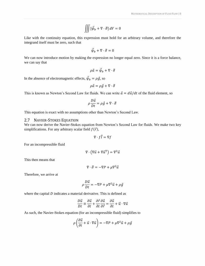
If �⃗⃗� ≠ 0 (and �⃗⃗� ≠ constant) then

�̿� = −𝑃I̿ + �̿�

where �̿� is sometimes called “extra stress” or more commonly “viscous stress”. It is nonzero if the fluid is

sheared or strained. An easier way to use this tensor is to note that

𝜎𝑖𝑗 = −𝑃𝛿𝑖𝑗 + 𝜏𝑖𝑗

where

𝜏𝑖𝑗 = 𝜇(∇𝑖𝑢𝑗 + ∇𝑗𝑢𝑖)


2.4 NEWTON’S LAW OF VISCOSITY When a simple fluid is sheared, it resists with the force (per unit area of the plane) which is proportional to

the gradient (i.e. derivative) of velocity. For general motion, this becomes

�̿� = 2𝜇�̿�

where 𝜇 is the viscosity and �̿� is the rate of strain tensor defined by

�̿� ≡1

2(∇�⃗⃗� + ∇�⃗⃗�T)

where the superscript T refers to the transpose. Therefore,

�̿� = −𝑃I̿ + 2𝜇�̿�

which is an approximate empirical relationship of Newtonian fluids, not valid for complicated fluids like

polymer solutions. Note that �̿� is symmetric such that 𝐸𝑖𝑗 = 𝐸𝑗𝑖. The term ∇�⃗⃗� is not the divergence of �⃗⃗�

since that would require a dot product. Rather, it represents the velocity gradient tensor, which is the

gradient operator applied to �⃗⃗�. In Cartesian coordinates this is

∇�⃗⃗� =

(

𝜕𝑢𝑥𝜕𝑥

𝜕𝑢𝑥𝜕𝑦 𝜕𝑢𝑥𝜕𝑧

𝜕𝑢𝑦

𝜕𝑥

𝜕𝑢𝑦

𝜕𝑦

𝜕𝑢𝑦

𝜕𝑧𝜕𝑢𝑧𝜕𝑥 𝜕𝑢𝑧𝜕𝑦

𝜕𝑢𝑧𝜕𝑧 )

There is a point of notation that should be discussed. We should note that multiplying two tensors can be

done via (�⃗��⃗⃗�)𝑖𝑗= 𝑎𝑖𝑏𝑗. This is also written as (�⃗�⨂�⃗⃗�)

𝑖𝑗= 𝑎𝑖𝑏𝑗. The ⨂ operator is often referred to as the

tensor product.

2.5 GENERALIZED GAUSS’ THEOREM Recall that the standard divergence theorem states that

∯𝑓 ⋅ �̂� 𝑑𝑆 =∭div(𝑓) 𝑑𝑉

We can write a generalized Gauss’ theorem that is as follows

∭∇(operation)(tensor)𝑑𝑉 =∯�̂�(operation)(tensor) 𝑑𝑆

Recall that a scalar is a tensor of rank 0, a vector is a tensor of rank 1, and then tensors we have described

here are rank 2. The (operation) term can be a variety of things, such as (dot product), (ordinary product),

(tensor product), or (cross product). In the case of (operation) = (dot product) and (tensor) = (vector) then

we arrive at the divergence theorem.

Let us consider an example of the generalized Gauss’ theorem. In this case, we will have (operation) =

(ordinary product) and (tensor) = (scalar). Therefore,

∫∇𝑓 𝑑𝑉 = ∮ �̂�𝑓 𝑑𝑆


In one-dimensional space between the points 𝑎 and 𝑏, the gradient operator is just ∇= 𝑥𝑑

𝑑𝑥 for a line in the

𝑥 dimension. We also note that 𝑑𝑉 = 𝑑𝑥 for this system. The lefthand term then becomes

∫∇𝑓 𝑑𝑉 = ∫𝑥𝑑𝑓

𝑑𝑥

𝑏

𝑎

𝑑𝑥 = ∫𝑥𝑑𝑓

𝑏

𝑎

Since there is no surface to integrate over, the righthand term becomes

∮�̂�𝑓 𝑑𝑆 = (𝑓|𝑥=𝑏 − 𝑓|𝑥=𝑎)�̂�

Therefore, equation the two expressions (and dropping the 𝑥 since we only have one dimension anyway)

∫𝑑𝑓

𝑏

𝑎

= 𝑓|𝑥=𝑏 − 𝑓|𝑥=𝑎

which is the fundamental theorem of calculus!

2.6 NEWTON’S EQUATION OF MOTION FOR A FLUID Recall that in an inertial frame, �⃗� = 𝑚�⃗�. This will apply to any fluid element so small that it can be

considered to have a single value of �⃗�. Let it be infinitesimally small. Then, 𝑚 = 𝜌 𝑑𝑉 and �⃗� = �⃗⃗� 𝑑𝑉,

where �⃗⃗� is the total (body and contact) force per unit volume. Then 𝜌�⃗� = �⃗⃗�.

If only gravity were present, then �⃗⃗� = 𝜌�⃗�, but we need to find contact force per unit volume given the

stress tensor field �̿�. Consider a continuum (e.g. fluid) at rest (�⃗⃗� = 0, �⃗� = 0) under the combined action of

some arbitrary body force field (not only gravity) and �̿�. Then, 0 = �⃗⃗� = �⃗⃗�𝑏 + �⃗⃗�𝑐 where the 𝑏 subscript is

for body force and 𝑐 subscript is for contact force. We also have that �⃗⃗�𝑏(𝑟) is known (imposed from things

such gravity, electromagnetic field, etc.) while �⃗⃗�𝑐(𝑟) depends only on �̿�(𝑟).

Any part of this continuum, enclosed in a volume 𝑉, is at rest, and so the total force acting on it must be

zero. Thus,

(total body force in 𝑉) + (sum of contact forces acting on matter in 𝑉 across surface 𝑆) = 0

This becomes

∭�⃗⃗�𝑏 𝑑𝑉 +∯𝑓𝑑𝑆 = 0

Substituting in for the force

∭�⃗⃗�𝑏 𝑑𝑉 +∯�̿� ⋅ �̂� 𝑑𝑆 = 0

Applying the divergence theorem

∭�⃗⃗�𝑏 𝑑𝑉 +∭∇ ⋅ �̿� 𝑑𝑉 = 0

Combing the integrals


∭[�⃗⃗�𝑏 + ∇ ⋅ �̿�] 𝑑𝑉 = 0

Like with the continuity equation, this expression must hold for an arbitrary volume, and therefore the

integrand itself must be zero, such that

�⃗⃗�𝑏 + ∇ ⋅ �̿� = 0

We can now introduce motion by making the expression no longer equal zero. Since it is a force balance,

we can say that

𝜌�⃗� = �⃗⃗�𝑏 + ∇ ⋅ �̿�

In the absence of electromagnetic effects, �⃗⃗�𝑏 = 𝜌�⃗�, so

𝜌�⃗� = 𝜌�⃗� + ∇ ⋅ �̿�

This is known as Newton’s Second Law for fluids. We can write �⃗� = 𝑑�⃗⃗�/𝑑𝑡 of the fluid element, so

𝜌𝐷�⃗⃗�

𝐷𝑡= 𝜌�⃗� + ∇ ⋅ �̿�

This equation is exact with no assumptions other than Newton’s Second Law.

2.7 NAVIER-STOKES EQUATION We can now derive the Navier-Stokes equation from Newton’s Second Law for fluids. We make two key

simplifications. For any arbitrary scalar field 𝑓(𝑟),

∇ ⋅ 𝑓𝐼 ̿ = ∇𝑓

For an incompressible fluid

∇ ⋅ (∇�⃗⃗� + ∇�⃗⃗�T) = ∇2�⃗⃗�

This then means that

∇ ⋅ �̿� = −∇𝑃 + 𝜇∇2�⃗⃗�

Therefore, we arrive at

𝜌𝐷�⃗⃗�

𝐷𝑡= −∇𝑃 + 𝜇∇2�⃗⃗� + 𝜌�⃗�

where the capital 𝐷 indicates a material derivative. This is defined as

𝐷�⃗⃗�

𝐷𝑡≡𝜕�⃗⃗�

𝜕𝑡+𝜕𝑟

𝜕𝑡

𝜕�⃗⃗�

𝜕𝑟=𝜕�⃗⃗�

𝜕𝑡+ �⃗⃗� ⋅ ∇�⃗⃗�

As such, the Navier-Stokes equation (for an incompressible fluid) simplifies to

𝜌 (𝜕�⃗⃗�

𝜕𝑡+ �⃗⃗� ⋅ ∇�⃗⃗�) = −∇𝑃 + 𝜇∇2�⃗⃗� + 𝜌�⃗�


2.8 SIMPLIFYING THE NAVIER-STOKES EQUATION

2.8.1 REDUCED PRESSURE The Navier-Stokes equation can often be written without explicit use of gravity terms through the use of a

modified pressure, 𝑃mod. Modified pressure can be used when the problem does not involve free surfaces

(e.g. water/air interface). The modified pressure is defined as

𝑃mod ≡ 𝑃 − 𝑃hydrostatic

where

𝑃hydrostatic = 𝜌�⃗� ⋅ 𝑟 + constant

Then,

𝑃 = 𝑃mod + 𝜌�⃗� ⋅ 𝑟 + constant

With this, the 𝜌�⃗� − ∇𝑃 term in the N-S equation becomes

𝜌𝑟 − ∇𝑃 = 𝜌�⃗� − ∇𝑃mod − 𝜌∇(�⃗� ⋅ 𝑟 + constant) = −∇𝑃mod

From this, we can see that we can neglect the gravity term in the N-S equation and replaced ∇𝑃 with ∇𝑃mod.

This means that

𝜌 (𝜕�⃗⃗�

𝜕𝑡+ �⃗⃗� ⋅ ∇�⃗⃗�) = −∇𝑃mod + 𝜇∇

2�⃗⃗�

Oftentimes, the “mod” subscript is omitted for brevity’s sake.

2.8.2 REYNOLDS NUMBER The Navier-Stokes equation can be written using only dimensionless quantities. A dimensionless variable

is defined as the original value divided by a given scale. For distances, you should use an appropriate length

given the boundary conditions and is denoted 𝐿. The dimensionless velocity is denoted 𝑢. The

dimensionless pressure is simply 𝜌𝑢2, and the dimensionless time is then 𝐿/𝑢. With these definitions, the

Navier-Stokes equation becomes the following

𝜕�⃗⃗�

𝜕𝑡+ �⃗⃗� ⋅ ∇�⃗⃗� = −∇𝑃 +

1

Re∇2�⃗⃗�

where Re is the Reynolds number is

Re ≡𝜌𝑢𝐿

𝜂=𝑢𝐿

ν

If the geometry of two problems is similar except for scale, and the Reynolds number is identical in both

cases, then the mathematical solutions, in scaled dimensionless variables, are identical. This is the basis

behind most “scale-up” studies.

2.8.3 APPROXIMATE SOLUTIONS OF THE NAVIER-STOKES EQUATION Generally, the forces on a given fluid are

−(inertia force) = (pressure force) + (viscous force)


where inertia force is simply −𝑚�⃗�. In many flows, the pressure force is mainly balanced by either the

inertial force or viscous force. The key question is when either of these terms can be neglected in the Navier-

Stokes equation. We will do this by estimating the ratio of

|𝜌𝐷�⃗⃗�𝐷𝑡 |

|𝜂∇2�⃗⃗�|

After all of the relevant quantities are made dimensionless, this ratio becomes the following (assuming

steady flow)

Re|𝐷�⃗⃗�𝐷𝑡 |

|∇2�⃗⃗�|= Re

|�⃗⃗� ⋅ ∇𝑣|

|∇2�⃗⃗�|

If Re ≪ 1, viscous forces are dominant, which is called Stokes flow, creeping flow, or low Reynolds flow.

This then means that the Navier-Stokes equation can be written as

0 = −∇𝑃 + 𝜂∇2�⃗⃗�

where the left-hand side of the Navier-Stokes equation is approximately zero under this assumption. Note

that this drops out the density term.

FORCES AND TORQUES: SPHERE IN STOKES FLOW | 11

3 FORCES AND TORQUES: SPHERE IN STOKES FLOW 3.1.1 PROBLEM SETUP Consider Stokes flow past a sphere of radius 𝑎. Far upstream, the flow is uniform with velocity 𝑈, and the

pressure there is 𝑃0. In the spherical coordinate system centered at the center of the sphere, the axis 𝜃 = 0

is along the direction of the incoming flow (which will be said to flow in the �̂� direction). It can be derived

(although it will simply be stated here) that the velocity profiles and pressure profile are

𝑢𝑟 = 𝑈 (1 −3

2

𝑎

𝑟+1

2(𝑎

𝑟)3

) cos𝜃

𝑢𝜃 = −𝑈(1 −3

4

𝑎

𝑟−1

4(𝑎

𝑟)3

) sin 𝜃

𝑢𝜙 = 0

and

𝑃 = 𝑃0 −3

2

𝜂𝑈

𝑎(𝑎

𝑟)2

cos 𝜃

The goal is to calculate the total force on the sphere from the fluid, which can be calculated as the sum of

the force due to the tangential stress on the surface of the sphere, the force from the viscous normal stress,

and the force on the sphere due to pressure. Why is this so? First, let’s write out the expression for force:

𝑓 = �̿� ⋅ �̂�

We know that the normal direction on the surface of the sphere is �̂�, so �̂� = �̂�. We can rewrite the force as

𝑓 = �̿� ⋅ �̂�

From symmetry, we can make the argument that the force has no 𝜙 component. Therefore,

𝑓 = 𝑓𝑟�̂� + 𝑓𝜃𝜃

where 𝑓𝑟 ≡ �̂� ⋅ 𝑓 and is the normal stress and 𝑓𝜃 ≡ 𝜃 ⋅ 𝑓 and is the tangential stress. We can now state that

𝑓𝑟 = �̂� ⋅ 𝑓 = �̂� ⋅ �̿� ⋅ �̂� = 𝜎𝑟𝑟 = −𝑃𝛿𝑟𝑟 + 𝜏𝑟𝑟 = −𝑃 + 2𝜂𝜕𝑢𝑟𝜕𝑟

We can also state that

𝑓𝜃 = 𝜃 ⋅ 𝑓 = 𝜃 ⋅ �̿� ⋅ �̂� = 𝜎𝜃𝑟 = −𝑃𝛿𝜃𝑟 + 𝜏𝜃𝑟 = 𝜂 (𝑟𝜕

𝜕𝑟(𝑢𝜃𝑟) +

1

𝑟

𝜕𝑢𝑟𝜕𝜃)

From this, we see that there are three components to the total force: the force due to tangential stress 𝜏𝜃𝑟,

the force due to normal stress 𝜏𝑟𝑟, and the force due to pressure.

3.1.2 FORCE DUE TO TANGENTIAL STRESS We now look at calculating the force due to the tangential stress, 𝜏𝜃𝑟. Therefore, we must first calculate the

tangential stress, which turns out to be


𝜏𝜃𝑟 = 𝜂 (𝑟𝜕


1

𝑟

𝜕𝑢𝑟𝜕𝜃) = −

3

2

𝜂𝑈 sin 𝜃

𝑎

The force due to tangential stress is then

�⃗� = ∯𝑓𝜃�̂� 𝑑𝑆 =∯𝜏𝜃𝑟 𝜃𝑑𝑆

It is difficult to do the surface integral of a vector, so some simplification must be made. By symmetry, we

can note that the force on the sphere will only act in the direction of flow (which we have defined as the �̂�

direction). Therefore, we can say multiply both sides by �̂�

�⃗� ⋅ �̂� = (∯𝜏𝜃𝑟 𝜃𝑑𝑆) ⋅ �̂�

Since �̂� is a constant, it can be pulled into the integrand (and we can note that 𝐹 = �⃗� ⋅ �̂�)

𝐹 =∯𝜏𝜃𝑟 𝜃 ⋅ �̂�𝑑𝑆

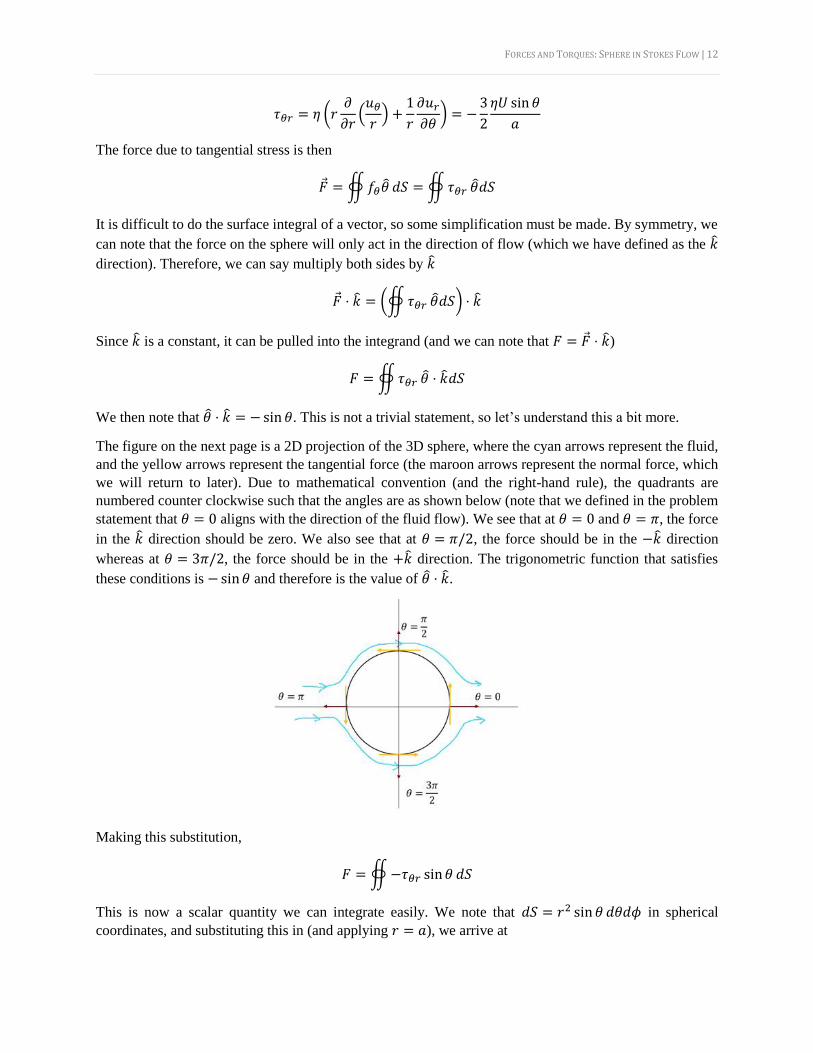
We then note that 𝜃 ⋅ �̂� = − sin 𝜃. This is not a trivial statement, so let’s understand this a bit more.

The figure on the next page is a 2D projection of the 3D sphere, where the cyan arrows represent the fluid,

and the yellow arrows represent the tangential force (the maroon arrows represent the normal force, which

we will return to later). Due to mathematical convention (and the right-hand rule), the quadrants are

numbered counter clockwise such that the angles are as shown below (note that we defined in the problem

statement that 𝜃 = 0 aligns with the direction of the fluid flow). We see that at 𝜃 = 0 and 𝜃 = 𝜋, the force

in the �̂� direction should be zero. We also see that at 𝜃 = 𝜋/2, the force should be in the −�̂� direction

whereas at 𝜃 = 3𝜋/2, the force should be in the +�̂� direction. The trigonometric function that satisfies

these conditions is −sin𝜃 and therefore is the value of 𝜃 ⋅ �̂�.

Making this substitution,

𝐹 =∯−𝜏𝜃𝑟 sin𝜃 𝑑𝑆

This is now a scalar quantity we can integrate easily. We note that 𝑑𝑆 = 𝑟2 sin 𝜃 𝑑𝜃𝑑𝜙 in spherical

coordinates, and substituting this in (and applying 𝑟 = 𝑎), we arrive at


𝐹 = ∫ ∫−𝜏𝜃𝑟 sin2 𝜃 𝑎2𝑑𝜃𝑑𝜙

𝜋

0

2𝜋

0

When we substituting in 𝜏𝜃𝑟 (evaluated at 𝑟 = 𝑎), we arrive at

𝐹 = ∫ ∫−(−3

2

𝜂𝑈 sin𝜃

𝑎) sin2 𝜃 𝑎2𝑑𝜃𝑑𝜙

𝜋

0

2𝜋

0

which simplifies to

𝐹 =3

2𝜂𝑈𝑎∫ ∫ sin3 𝜃 𝑑𝜃𝑑𝜙

𝜋

0

2𝜋

0

This becomes

𝐹 = 3𝜂𝑈𝑎𝜋∫ sin3 𝜃 𝑑𝜃

𝜋

0

We can split this into

𝐹 = 3𝜂𝑈𝑎𝜋∫ sin2 𝜃 sin 𝜃 𝑑𝜃

𝜋

0

By using a trigonometric identity,

𝐹 = 3𝜂𝑈𝑎𝜋∫(1 − cos2 𝜃) sin 𝜃 𝑑𝜃

𝜋

0

By using the substitution 𝜉 = cos 𝜃 and 𝑑𝜉 = −sin 𝜃 𝑑𝜃 we can say that that

𝐹 = −3𝜂𝑈𝑎𝜋 ∫ (𝜉2 − 1)𝑑𝜉

𝜃=𝜋

𝜃=0

which becomes

𝐹 = 4𝜋𝜂𝑈𝑎

Assigning the sign yields

�⃗� = 4𝜋𝜂𝑈𝑎 �̂�

3.1.3 FORCE DUE TO VISCOUS NORMAL STRESS The total force in the 𝑟 direction can be found by

�⃗� = ∯𝑓𝑟�̂� 𝑑𝑆

Substituting in the value of 𝑓𝑟 yields


�⃗� = ∯(−𝑃 + 𝜏𝑟𝑟)�̂� 𝑑𝑆

This can be split up into two parts:

�⃗� = ∯−𝑃�̂� 𝑑𝑆 +∯𝜏𝑟𝑟�̂� 𝑑𝑆

The right integral is the force due to the viscous normal stress and will be determined in this part of the

problem. Just to be rigorous, we once again note that it is difficult to calculate the surface integral of a

vector and must multiply both sides by �̂�, the direction of the force. As such,

𝐹 = �⃗� ⋅ �̂� = ∯−𝑃�̂� ⋅ �̂� 𝑑𝑆 +∯𝜏𝑟𝑟�̂� ⋅ �̂� 𝑑𝑆

The left integral is the force due to pressure, and the right integral is the force due to the viscous normal

stress. I will focus on the force due to the viscous normal stress in this subsection. It can be calculated by

𝜏𝑟𝑟 = 2𝜂𝜕𝑢𝑟𝜕𝑟

By evaluating this at 𝑟 = 𝑎, we arrive at

𝜏𝑟𝑟 = 0

Therefore, when we go to calculate the force due to the viscous normal stress, we would find that

∯𝜏𝑟𝑟 �̂� ⋅ �̂� 𝑑𝑆 = 0

and so there is no contribution from the viscous normal stress.

3.1.4 FORCE DUE TO PRESSURE We will now calculate the force due to pressure (i.e. the left surface integral in the previous subsection). It

was explicitly derived in the previous subsection, but I will drive this point home by recalling that 𝑓 =

−𝑃�̂�. As such, since �̂� = �̂� and since we must convert the vector to a scalar for integration purposes, we

arrive at the same result as in the prior subsection

𝐹 =∯−𝑃�̂� ⋅ �̂� 𝑑𝑆

We can now note that �̂� ⋅ �̂� = cos 𝜃. Once again, this is not a trivial point, but it can be determined from

the previous figure by focusing on the maroon arrows that represent the normal force. We see that the value

of the force should align with �̂� at 𝜃 = 0 and be in the direction of −�̂� at 𝜃 = 𝜋. Further, we see that at

𝜃 = 𝜋/2 and 𝜃 = 3𝜋/2, the normal force is orthogonal to the direction of fluid flow and therefore has no

component in the �̂� direction. The appropriate trigonometric function for this is cos 𝜃.

Applying this identity,

𝐹 =∯−𝑃cos 𝜃 𝑑𝑆

We recall that 𝑑𝑆 = 𝑟2 sin 𝜃 𝑑𝜃𝑑𝜙 in spherical coordinates. Substituting this in and making 𝑟 = 𝑎, we

arrive at


𝐹 = ∫ ∫−𝑃 cos𝜃 𝑎2 sin𝜃 𝑑𝜃𝑑𝜙

𝜋

0

2𝜋

0

Substituting in for the pressure

𝐹 = ∫ ∫−(𝑃0 −3

2

𝜂𝑈

𝑎cos 𝜃) cos𝜃 𝑎2 sin𝜃 𝑑𝜃𝑑𝜙

𝜋

0

2𝜋

0

This simplifies to

𝐹 = ∫ ∫3

2𝜂𝑈𝑎 cos2 𝜃 sin 𝜃

𝜋

0

𝑑𝜃𝑑𝜙

2𝜋

0

−∫ ∫𝑃0𝑎 cos𝜃 sin𝜃 𝑑𝜃𝑑𝜙

𝜋

0

2𝜋

0

The right term goes to zero because the integral of an odd function over a symmetric range is zero (or you

can calculate it yourself to find out). This means that

𝐹 = ∫ ∫3

2𝜂𝑈𝑎 cos2 𝜃 sin 𝜃

𝜋

0

𝑑𝜃𝑑𝜙

2𝜋

0

This becomes

𝐹 = 3𝜋𝜂𝑈𝑎∫ cos2 𝜃 sin𝜃 𝑑𝜃

𝜋

0

By using the substitution 𝜉 = cos 𝜃 and 𝑑𝜉 = −sin 𝜃 𝑑𝜃, we can integrate the expression with ease to yield

𝐹 = 2𝜋𝜂𝑈𝑎

If we apply the direction now we arrive at

�⃗� = 2𝜋𝜂𝑈𝑎 �̂�

3.1.5 TOTAL FORCE ON THE SPHERE FROM THE FLUID The total force on the sphere from the fluid is the sum of the forces in the prior three sections. As such, the

total force is simply

�⃗� = 6𝜋𝜂𝑈𝑎 �̂�

This is often referred to as Stokes’ formula.

ONE-DIMENSIONAL FLOW IN VISCOUS FLUIDS | 16

4 ONE-DIMENSIONAL FLOW IN VISCOUS FLUIDS 4.1 POISEUILLE FLOW Let us consider the steady flow of an incompressible fluid through a horizontal cylinder of length 𝐿 and

radius 𝑎. The goal is to find the velocity profile, mean velocity, and volumetric flow rate.

In this problem, I will use cylindrical (𝑟, 𝜃, 𝑧) components. The 𝑧 direction will be the direction down the

pipe. The value of 𝑟 = 0 will be set to be in the middle of the cylindrical pipe. With this set of definitions,

we have that �⃗⃗� = 𝑢𝑧 (i.e. 𝑢𝑟 = 𝑢𝜃 = 0). We also postulate that 𝑢𝑧(𝑟).

We start with the continuity equation:

𝜕𝜌

𝜕𝑡+ ∇ ⋅ 𝜌�⃗⃗� = 0

Assuming that 𝜌 is constant, this simply becomes

∇ ⋅ �⃗⃗� = 0

which in cylindrical coordinates is

1

𝑟

𝜕

𝜕𝑟(𝑟𝑢𝑟) +

1

𝑟

𝜕

𝜕𝜃(𝑢𝜃) +

𝜕

𝜕𝑧(𝑢𝑧) = 0

This simplifies to

𝜕𝑢𝑧𝜕𝑧

= 0

Now, let us write the Navier-Stokes equation. Ignoring the effect of gravity,

𝜌 (𝜕�⃗⃗�

𝜕𝑡+ �⃗⃗� ⋅ ∇�⃗⃗�) = −∇𝑃 + 𝜂∇2�⃗⃗�

In cylindrical coordinates this becomes,

𝜌 (𝜕𝑢𝑧𝜕𝑡+ 𝑢𝑟

𝜕𝑢𝑧𝜕𝑟

+𝑢𝜃𝑟

𝜕𝑢𝑧𝜕𝜃

+ 𝑢𝑧𝜕𝑢𝑧𝜕𝑧) = −

𝜕𝑃

𝜕𝑧+ 𝜂 (

1

𝑟

𝜕

𝜕𝑟(𝑟𝜕𝑢𝑧𝜕𝑟) +

1

𝑟2𝜕2𝑢𝑧𝜕𝜃2

+𝜕2𝑢𝑧𝜕𝑧2

)

We employ the previous assumptions. Also, we note that the pressure differential can be well-approximated

by a linear pressure drop, Δ𝑃, which is conventionally defined to be a positive quantity. As such,

𝑑𝑃

𝑑𝑧=𝑃2 − 𝑃1𝐿

= −Δ𝑃

𝐿

As such, the Navier-Stokes equation can be simplified to the following form

0 =Δ𝑃

𝐿+ 𝜂 (

1

𝑟

𝜕

𝜕𝑟(𝑟𝜕𝑢𝑧𝜕𝑟))

Rearranging the above expression yields

−Δ𝑃

𝜂𝐿𝑟 =

𝜕

𝜕𝑟(𝑟𝜕𝑢𝑧𝜕𝑟)


Integrating twice yields

𝑢𝑧 = −Δ𝑃

𝜂𝐿

𝑟2

4+ 𝐶1 ln(𝑟) + 𝐶2

We have to employ boundary conditions now. We know that at 𝑟 = 0, the velocity should be finite. As

such, we can immediately say that 𝐶1 = 0. Therefore,

𝑢𝑧 = −Δ𝑃

𝜂𝐿

𝑟2

4+ 𝐶2

The other condition is that at 𝑟 = 𝑎, the no-slip boundary condition applies and 𝑢𝑧 = 0. We then have that

𝐶2 =Δ𝑃

𝜂𝐿

𝑎2

4

such that

𝑢𝑧 =Δ𝑃

4𝜂𝐿(𝑎2 − 𝑟2)

The mean velocity can be calculated by dividing the total volumetric flow rate by the cross-sectional area

via

⟨𝑢𝑧⟩ =∬𝑢𝑧 𝑑𝐴

∬𝑑𝐴

This becomes

⟨𝑢𝑧⟩ =∫ ∫ 𝑢𝑧 𝑟𝑑𝑟𝑑𝜃

𝑎

0

2𝜋

0

∫ ∫ 𝑟𝑑𝑟𝑑𝜃𝑎

0

2𝜋

0

=

𝜋𝑎4Δ𝑝8𝜂𝐿

𝜋𝑎2=𝑎2Δ𝑃

8𝜂𝐿

The mean velocity in the cross-section is then

⟨𝑢𝑧⟩ =𝑎2Δ𝑃

8𝜂𝐿

The total (volumetric) flow rate can be found by multiplying the mean velocity in the cross-section by the

cross-sectional area

𝑄 =∬⟨𝑢𝑧⟩ 𝑑𝐴 = ∫ ∫⟨𝑢𝑧⟩

𝑎

0

𝑟𝑑𝑟𝑑𝜃

2𝜋

0

=𝜋𝑎4Δ𝑃

8𝜂𝐿

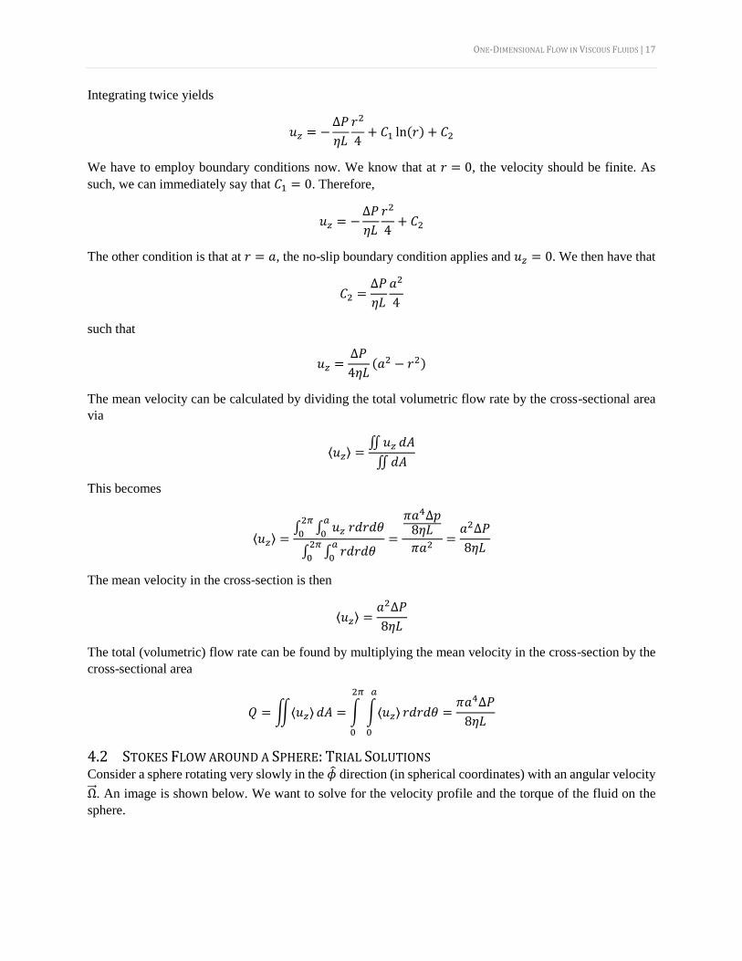
4.2 STOKES FLOW AROUND A SPHERE: TRIAL SOLUTIONS Consider a sphere rotating very slowly in the �̂� direction (in spherical coordinates) with an angular velocity

Ω⃗⃗⃗. An image is shown below. We want to solve for the velocity profile and the torque of the fluid on the

sphere.


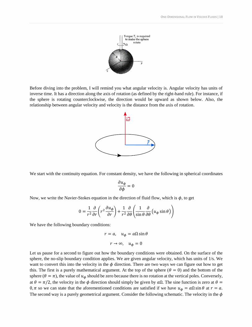
Before diving into the problem, I will remind you what angular velocity is. Angular velocity has units of

inverse time. It has a direction along the axis of rotation (as defined by the right-hand rule). For instance, if

the sphere is rotating counterclockwise, the direction would be upward as shown below. Also, the

relationship between angular velocity and velocity is the distance from the axis of rotation.

We start with the continuity equation. For constant density, we have the following in spherical coordinates

𝜕𝑢𝜙

𝜕𝜙= 0

Now, we write the Navier-Stokes equation in the direction of fluid flow, which is 𝜙, to get

0 =1

𝑟2𝜕

𝜕𝑟(𝑟2

𝜕𝑢𝜙

𝜕𝑟) +

1

𝑟2𝜕

𝜕𝜃(1

sin 𝜃

𝜕

𝜕𝜃(𝑢𝜙 sin𝜃))

We have the following boundary conditions:

𝑟 = 𝑎, 𝑢𝜙 = 𝑎Ω sin𝜃

𝑟 → ∞, 𝑢𝜙 = 0

Let us pause for a second to figure out how the boundary conditions were obtained. On the surface of the

sphere, the no-slip boundary condition applies. We are given angular velocity, which has units of 1/s. We

want to convert this into the velocity in the 𝜙 direction. There are two ways we can figure out how to get

this. The first is a purely mathematical argument. At the top of the sphere (𝜃 = 0) and the bottom of the

sphere (𝜃 = 𝜋), the value of 𝑢𝜙 should be zero because there is no rotation at the vertical poles. Conversely,

at 𝜃 = 𝜋/2, the velocity in the 𝜙 direction should simply be given by 𝑎Ω. The sine function is zero at 𝜃 =

0, 𝜋 so we can state that the aforementioned conditions are satisfied if we have 𝑢𝜙 = 𝑎Ωsin𝜃 at 𝑟 = 𝑎.

The second way is a purely geometrical argument. Consider the following schematic. The velocity in the 𝜙


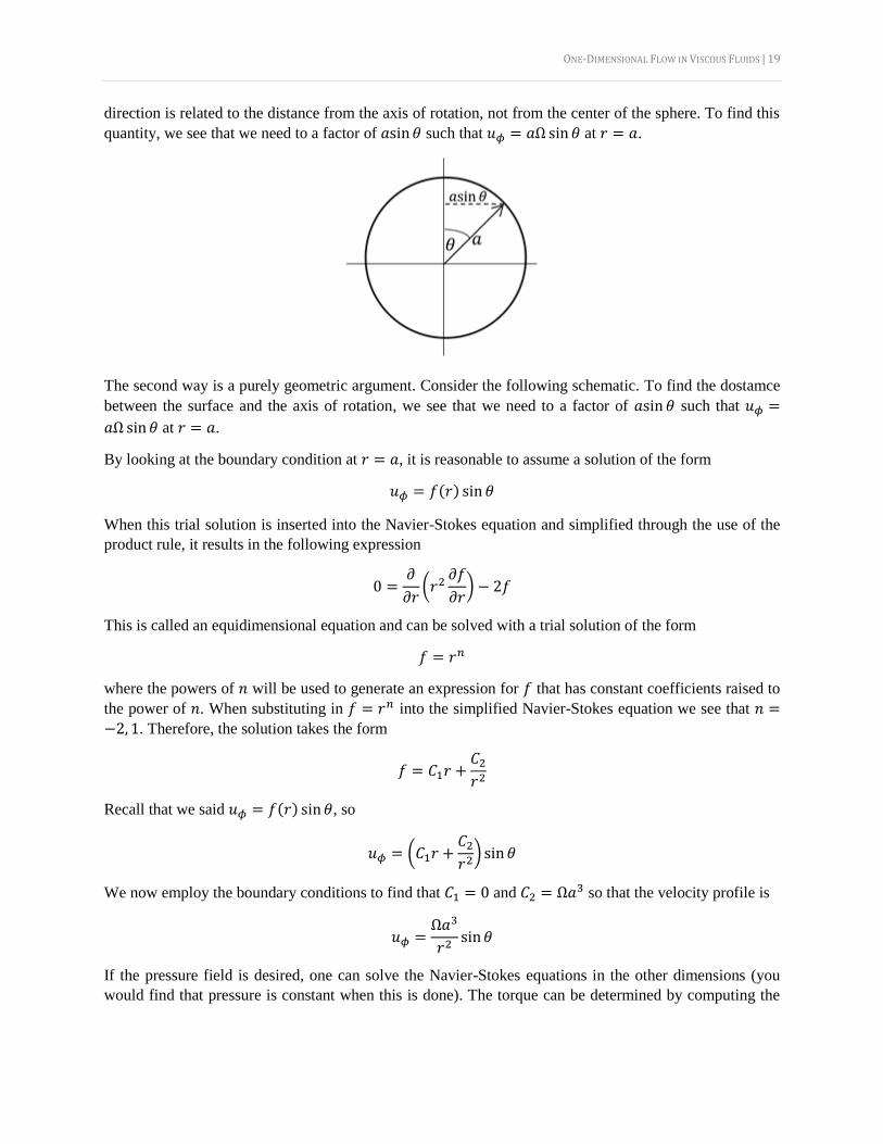
direction is related to the distance from the axis of rotation, not from the center of the sphere. To find this

quantity, we see that we need to a factor of 𝑎sin𝜃 such that 𝑢𝜙 = 𝑎Ω sin 𝜃 at 𝑟 = 𝑎.

The second way is a purely geometric argument. Consider the following schematic. To find the dostamce

between the surface and the axis of rotation, we see that we need to a factor of 𝑎sin 𝜃 such that 𝑢𝜙 =

𝑎Ω sin 𝜃 at 𝑟 = 𝑎.

By looking at the boundary condition at 𝑟 = 𝑎, it is reasonable to assume a solution of the form

𝑢𝜙 = 𝑓(𝑟) sin 𝜃

When this trial solution is inserted into the Navier-Stokes equation and simplified through the use of the

product rule, it results in the following expression

0 =𝜕

𝜕𝑟(𝑟2

𝜕𝑓

𝜕𝑟) − 2𝑓

This is called an equidimensional equation and can be solved with a trial solution of the form

𝑓 = 𝑟𝑛

where the powers of 𝑛 will be used to generate an expression for 𝑓 that has constant coefficients raised to

the power of 𝑛. When substituting in 𝑓 = 𝑟𝑛 into the simplified Navier-Stokes equation we see that 𝑛 =

−2, 1. Therefore, the solution takes the form

𝑓 = 𝐶1𝑟 +𝐶2𝑟2

Recall that we said 𝑢𝜙 = 𝑓(𝑟) sin𝜃, so

𝑢𝜙 = (𝐶1𝑟 +𝐶2𝑟2) sin 𝜃

We now employ the boundary conditions to find that 𝐶1 = 0 and 𝐶2 = Ω𝑎3 so that the velocity profile is

𝑢𝜙 =Ω𝑎3

𝑟2sin𝜃

If the pressure field is desired, one can solve the Navier-Stokes equations in the other dimensions (you

would find that pressure is constant when this is done). The torque can be determined by computing the


stress, multiplying it by the lever arm, and then integrating over the surface of the sphere. Since we have

flow in the 𝜙 direction that is a function of 𝑟, we want the stress that is 𝜏𝑟𝜙 which is

𝜏𝑟𝜙 = 𝜂𝑟𝜕

𝜕𝑟(𝑢𝜙

𝑟)

in our case once the simplifications are made. You can plug in the velocity distribution and apply 𝑟 = 𝑎

(since we want the stress at the surface) to get

𝜏𝑟𝜙|𝑟=𝑎= −3𝜂Ωsin𝜃

The lever arm is given by 𝑎sin 𝜃, so the torque can be found by

𝐾 =∯𝜏𝑟𝜙|𝑟=𝑎(𝑎 sin𝜃) 𝑑𝑆

Once this computation is performed, you arrive at

𝐾 = −8𝜋𝜂Ω𝑎3

Of course, torque is a vector, and it needs a direction. It will be in the direction of the angular velocity. As

such,

�⃗⃗⃗� = −8𝜋𝜂Ω⃗⃗⃗𝑎3

4.3 PLATE SUDDENLY SET IN MOTION: TIME-DEPENDENT FLOW Consider a semi-infinite body of liquid at a constant density and viscosity that is sitting atop a horizontal

plate in the 𝑥𝑧 plane. The plate is suddenly set into motion at a velocity 𝑢0, causing a fluid velocity profile

that changes in both time and in 𝑦, the vertical distance from the plate. The goal is to find the velocity

profile.

As always, we start with the Navier-Stokes equation

𝜌 (𝜕�⃗⃗�

𝜕𝑡+ �⃗⃗� ⋅ ∇�⃗⃗�) = −∇𝑃 + 𝜂∇2�⃗⃗� + 𝜌�⃗�

The fluid velocity is �⃗⃗� = 𝑢𝑥(𝑦, 𝑡). Therefore, the above equation simplifies to the following once relevant

terms are canceled in the Navier-Stokes equation:

𝜕𝑢𝑥𝜕𝑡

= 𝜈𝜕2𝑢𝑥𝜕𝑦2

where 𝜈 ≡ 𝜂/𝜌. We have the following conditions:

𝑡 ≤ 0, 𝑢𝑥 = 0

𝑦 = 0, 𝑢𝑥 = 𝑢0

𝑦 = ∞, 𝑢𝑥 = 0

To solve this, we need to first introduce a non-dimensional quantity for the velocity. I will define the non-

dimensional velocity as


𝜙 ≡𝑢𝑥𝑢0

The boundary conditions now become the following for 𝜙(𝑦, 𝑡)

𝜙(𝑦, 0) = 0, 𝜙(0, 𝑡) = 1, 𝜙(∞, 𝑡) = 0

We know that 𝜙 should be a quantity that is proportional to 𝑦, 𝑡, and 𝜈 (our independent and dependent

variables in the simplified Navier-Stokes equation). We can then say that

𝜙 = 𝜙(𝜂)

where

𝜂 ≡𝑦

√4𝜈𝑡

It should be apparent that the dimensions of 𝜂 are indeed unitless. I have included the factor of 4 because I

know what the answer is going to be in advance and it simplifies the algebra. This step is not necessary and

does not change the validity of the solution. With these expressions, we can rewrite the partial differential

equation as

𝜕𝜙

𝜕𝑡= 𝜈

𝜕2𝜙

𝜕𝑦2

Let’s break this down part by part. For the time component we can say that

𝜕𝜙

𝜕𝑡=𝑑𝜙

𝑑𝜂

𝜕𝜂

𝜕𝑡= −

1

2

𝜂

𝑡

𝑑𝜙

𝑑𝜂

For the 𝑦 component we can say that

𝜕𝜙

𝜕𝑦=𝑑𝜙

𝑑𝜂

𝜕𝜂

𝜕𝑦=𝑑𝜙

𝑑𝜂

1

√4𝜈𝑡

Therefore,

𝜕2𝜙

𝜕𝑦2=𝑑2𝜙

𝑑𝑦21

4𝜈𝑡

This makes the N-S equation become

𝑑2𝜙

𝑑𝜂2+ 2𝜂

𝑑𝜙

𝑑𝜂= 0

If I tentatively define

𝜓 ≡𝑑𝜙

𝑑𝜂

such that

𝑑𝜓

𝑑𝜂+ 2𝜂𝜓 = 0


we can then rearrange this to

1

𝜓𝑑𝜓 = −2𝜂 𝑑𝜂

and integrate once to get

𝜓 = 𝐶1 exp(−𝜂2)

Transforming this back to our prior set of variables,

𝑑𝜙

𝑑𝜂= 𝐶1 exp(−𝜂

2)

And integrating one final time yields

𝜙 = 𝐶1∫exp(−�̅�2) 𝑑�̅�

𝜂

0

+ 𝐶2

where I have set �̅� to be a dummy variable of integration to distinguish it from 𝜂 in our integral’s bounds.

The boundary conditions are

𝜂 = 0, 𝜙 = 1

𝜂 = ∞, 𝜙 = 0

Applying these boundary conditions yields the following after some algebra,

𝜙 = 1 −∫ exp(−�̅�2)𝜂

0𝑑�̅�

∫ exp(−�̅�2)∞

0𝑑�̅�= 1 −

2

√𝜋∫ exp(−�̅�2) 𝑑�̅�

𝜂

0

= 1 − erf(𝜂) = erfc(η)

This solution makes use of the error function, denoted erf, but do not let this scare you – it is simply a short-

hand way of expressing the otherwise messy integral shown above. The complementary error function,

erfc, is simply 1 minus the error function. With this, we can transform 𝜙 back to our original variables to

arrive at

𝑢𝑥 = 𝑢0 erfc (𝑦

√4𝜈𝑡)

VORTICITY | 23

5 VORTICITY 5.1 DEFINITION OF VORTICITY Vorticity is defined as

�⃗⃗⃗� = ∇×�⃗⃗�

The vorticity indicates the local rate of rotation of a fluid element. Generally, it is different from point to

point. The surface integral of a curl can be related to the line integral of velocity via Stokes’ theorem (see

Appendix):

∯�⃗⃗⃗� ⋅ �̂� 𝑑𝑆 = ∮ �⃗⃗� ⋅ 𝑑𝑟

The line integral of velocity is also called the circulation of velocity (over a given boundary). To test this

formula out, consider a disk in rotation with a radius 𝑎. The above expression then lets us say that

�⃗⃗⃗�𝜋𝑎2 = (Ω⃗⃗⃗𝑎)2𝜋𝑎

such that

�⃗⃗⃗� = 2Ω⃗⃗⃗

To clarify, the left-hand side of the first equation is vorticity multiplied by the surface area of the disk

whereas the right-hand side of the first equation is the velocity multiplied by the circumference of the disk.

In the following sections, we will find that

1. Vorticity is generated on solid surfaces due to no-slip boundary condition

2. Vorticity “diffuses” due to viscosity

3. Vorticity is swept downstream due to convection

5.2 CURL OF NAVIER-STOKES The curl of the Navier-Stokes equation (in dimensionless form) is the following:

𝜕�⃗⃗⃗�

𝜕𝑡+ �⃗⃗� ⋅ ∇�⃗⃗⃗� = �⃗⃗⃗� ⋅ ∇�⃗⃗� +

1

Re∇2�⃗⃗⃗�

In a 2D or axisymmetric flow, we have that �⃗⃗⃗� ⋅ ∇�⃗⃗� = 0, so the Navier-Stokes equation becomes

𝜕�⃗⃗⃗�

𝜕𝑡+ �⃗⃗� ⋅ ∇�⃗⃗⃗� =

1

Re∇2�⃗⃗⃗�

5.3 LOW REYNOLDS NUMBER One extreme case we will consider is when the Reynolds number is very small (approaching zero), such as

with creeping flow. Recall that this is the same as creeping flow, so the entire left-hand side of the (velocity-

pressure form) Navier-Stokes equation drops out. When dealing with the vorticity form, since convection

is negligible, nd we can write the Navier-Stokes equation in dimensional variables as follows

𝜕�⃗⃗⃗�

𝜕𝑡=𝜂

𝜌∇2�⃗⃗⃗�

where 𝜂/𝜌 is the kinematic viscosity, often denoted 𝜈. This equation is that of the diffusion equation. Of

course, if the vorticity does not change with time we arrive at

VORTICITY | 24

∇2�⃗⃗⃗� = 0

This essentially means that for creeping flow with low Reynolds number, and the vorticity looks like the

following where each line represents a constant vorticity contour line and the flow comes from the left.

5.4 HIGH REYNOLDS NUMBER If the Reynolds number is very large (approaching infinity),

1

Re∇2�⃗⃗⃗� can be ignored, and the Navier-Stokes

equation simplifies to

𝜕�⃗⃗⃗�

𝜕𝑡+ �⃗⃗� ⋅ ∇�⃗⃗⃗� = 0

which is the same as

𝐷�⃗⃗⃗�

𝐷𝑡= 0

This states that the vorticity is conserved (i.e. it remains constant) in each moving fluid element. In a steady

flow, the vorticity is then constant along a given streamline. When the Reynolds number is high, we have

increasing convection, and the vorticity field around an arbitrary body looks as follow, with �⃗⃗⃗� = 0 outside

the boundary layer and wake but �⃗⃗⃗� ≠ 0 inside the boundary layer and wake.

While the above form of the Navier-Stokes equation tells us physical information about the vorticity, it is

not incredibly useful for gaining information about the velocity profiles since the boundary conditions for

vorticity are not straightforward. We would also like to write the velocity-pressure form of the Navier-

Stokes equation but in a way that accounts for regions of irrotational flow.

From vector calculus (see Appendix) and under the conditions of no divergence of velocity, we know that

the following is true

∇2�⃗⃗� = −∇×(∇×�⃗⃗�) = −∇×�⃗⃗⃗�

This is an important quantity to know because then we can say that in irritational flow, where �⃗⃗⃗� = 0, the

viscous force 𝜂∇2�⃗⃗� = 0 for any value of viscosity (of course, this also holds true if the viscosity is

incredibly small) even though the viscous stresses are not necessarily zero. Therefore, outside the boundary

layer and wake where there is irrotational flow, we can say that the Navier-Stokes equation simplifies to

VORTICITY | 25

𝜌 (𝜕�⃗⃗�

𝜕𝑡+ �⃗⃗� ⋅ ∇�⃗⃗�) = −∇𝑃 + 𝜌�⃗�

In steady flow, the time derivative goes away to yield

𝜌(�⃗⃗� ⋅ ∇�⃗⃗�) = −∇𝑃 + 𝜌�⃗�

This equation is called Euler’s equation. After a bit of vector calculus and algebra which has been omitted

here for brevity, we can arrive at

𝑢2

2+𝑃

𝜌+ 𝑔𝑧 = constant

throughout the irrotational flow areas. This formula is called Bernoulli’s theorem.

In regions with irrotational flow (also known as potential flow), we can define 𝜙 as the velocity potential

such that

�⃗⃗� ≡ ∇𝜙

This holds because the curl of velocity is zero. Then, from the continuity equation we can say that

∇ ⋅ �⃗⃗� = 0

which implies

∇2𝜙 = 0

5.5 CIRCULATION Suppose a closed curve made up of fluid particles and moving with a fluid where the viscous force is zero

or negligible at all points along it. Consider the circulation of velocity along the curve:

circulation = ∮ �⃗⃗� ⋅ 𝑑𝑟

We would like to know how the circulation changes with time, or

𝑑

𝑑𝑡∮ �⃗⃗� ⋅ 𝑑𝑟

We can distribute the derivative inside and then note that the derivative of the position vector is velocity

∮𝑑

𝑑𝑡(�⃗⃗� ⋅ 𝑑𝑟) =

𝑑�⃗⃗�

𝑑𝑡⋅ 𝑑𝑟 + �⃗⃗� ⋅

𝑑

𝑑𝑡(𝑑𝑟) =

𝑑�⃗⃗�

𝑑𝑡⋅ 𝑑𝑟 + �⃗⃗� ⋅ 𝑑�⃗⃗� =

𝑑�⃗⃗�

𝑑𝑡⋅ 𝑑𝑟 + 𝑑 (

1

2�⃗⃗� ⋅ �⃗⃗�)

Therefore,

𝑑

𝑑𝑡∮ �⃗⃗� ⋅ 𝑑𝑟 =

𝑑�⃗⃗�

𝑑𝑡⋅ 𝑑𝑟 + 𝑑 (

1

2�⃗⃗�2)

We then note that ∮𝑑𝑓 = 0 for any single-value function. Thus, in general, for any closed curve

𝑑

𝑑𝑡∮ �⃗⃗� ⋅ 𝑑𝑟 = ∮

𝑑�⃗⃗�

𝑑𝑡⋅ 𝑑𝑟

VORTICITY | 26

This says that the time derivative of circulation of velocity over a closed curve is equal to the circulation of

acceleration over the same curve. If on the curve, the viscous force −𝜈∇×�⃗⃗⃗� is negligible then

𝑑�⃗⃗�

𝑑𝑡= −

1

𝜌∇𝑃

Therefore, plugging this into the rate of change of circulation from above (and if 𝜌 is constant)

𝑑

𝑑𝑡∮ �⃗⃗� ⋅ 𝑑𝑟 = −∮

1

𝜌∇𝑃 ⋅ 𝑑𝑟 = −

1

𝜌∮𝑑𝑃 = 0

Therefore, if 𝜌 is constant, the circulation does not change. This is known as Kelvin’s theorem.

BOUNDARY LAYER THEORY | 27

6 BOUNDARY LAYER THEORY 6.1 HIGH REYNOLDS NUMBER FLOW OVER A FLAT PLATE PARALLEL TO FLOW Recall from transport phenomena that the vorticity diffusion due to viscosity can be thought of as

(penetration depth of vorticity diffusion over time 𝑡) ∼ √𝜈𝑡

This relationship will prove quite useful.

Consider a flat plate of very small thickness and a length ℓ. It is placed in a steady uniform stream of fluid

(with speed 𝑈), with the stream parallel to the length. In the absence of any effects of viscosity, the plate

causes no disturbance to the stream and the fluid velocity is uniform. However, real fluids have no-slip

boundary conditions that slow down the fluid near the liquid-solid interface. The boundary layer thickness

will be small compared to length 𝑙 provided that ℓ𝑈/𝜈 ≫ 1. The velocity just outside the boundary layer is

effectively unchanged and is therefore equal to 𝑈. The pressure outside the boundary layer is also uniform

and is approximately uniform throughout the boundary layer as well. We can postulate that the boundary

layer thickness would be given by1

𝛿 ∼ √𝜈𝑡 ∼ √𝜈𝑥/𝑈

This then says that the further away from the leading edge of the plate you are, the larger the boundary layer

thickness, as would be expected. The stress can be estimated as

𝜏wall ∼𝜂𝑈

𝛿∼ 𝜂𝑈

32𝜈−

12𝑥−

12 ∼ 𝜌𝜈

12𝑈

32𝑥−

12

The exact solution is

𝜏wall = 𝜂 (𝜕𝑢

𝜕𝑦)𝑦=0

= 0.33𝜌𝜈12𝑈

32𝑥−

12 = 0.33𝜂𝑈 (

𝑈

𝜈𝑥)

12

The velocity can be found from the stress by integrating, which yields

𝑢 = 0.33𝜈−12𝑈

32𝑥−

12𝑦 + 𝐶

To find the constant, we employ the no-slip boundary condition, which yields 𝐶 = 0.

𝑢 = 0.33𝜈−12𝑈

32𝑥−

12𝑦

The drag force per unit length exerted on the two sides of the plate is given by

𝐹𝐷,per width = 2∫𝜏wall

ℓ

0

𝑑𝑥 = 1.33𝜌𝜈12𝑈

32𝐿12

As such, the drag force on a plate of width 𝐿, that becomes2

𝐹𝐷 = 1.33𝜌𝜈12𝑈

32𝐿32

1 Note that if we have a disk spinning in a fluid, we replace 𝑈 with Ω𝑥 to arrive at 𝛿 ∼ √𝜈/Ω.

2 More generally, for a width 𝑊, it is 𝐹𝐷 = 1.33𝜌𝜈1

2𝑈3

2𝑊𝐿1

2


If one wants to write the boundary layer equations (the analogous to the Navier-Stokes equation), we note

that the velocity gradient in the 𝑥 direction is significantly smaller than that in the 𝑦 direction. If we start

with the Navier-Stokes equation in the 𝑥 direction as

𝜌 (𝑢𝑥𝜕𝑢𝑥𝜕𝑥

+ 𝑢𝑦𝜕𝑢𝑥𝜕𝑦) = −

𝜕𝑃

𝜕𝑥+ 𝜂 (

𝜕2𝑢𝑥𝜕𝑥2

+𝜕2𝑢𝑥𝜕𝑦2

)

we will see that the 𝜕2𝑢𝑥/𝜕𝑥2 term in the Laplacian can be ignored since the velocity gradient in 𝑥 is small.

Note that the 𝜕𝑢𝑥

𝜕𝑥 term in the left-hand side of the equation cannot be dropped because 𝑢𝑦 is small and

therefore 𝑢𝑥 𝜕𝑢𝑥/𝜕𝑥 is not significantly smaller than 𝑢𝑦 𝜕𝑢𝑥/𝜕𝑦. Therefore,

𝑢𝑥𝜕𝑢𝑥𝜕𝑥

+ 𝑢𝑦𝜕𝑢𝑥𝜕𝑦

− 𝜈𝜕2𝑢𝑥𝜕𝑦2

= −1

𝜌

𝜕𝑃

𝜕𝑥

From Bernoulli’s equation, we know that 𝑃 +1

2𝜌𝑈2 = constant. Taking the 𝑥 derivative of both sides

yields

𝑑𝑃

𝑑𝑥=𝑑 (12𝜌𝑈

2 + 𝐶)

𝑑𝑥

This becomes

𝑑𝑃

𝑑𝑥= −𝜌𝑈

𝑑𝑈

𝑑𝑥

We can substitute this into the boundary layer equation to arrive at



− 𝜈𝜕2𝑢𝑥𝜕𝑦2

= 𝑈𝑑𝑈

𝑑𝑥

If 𝑈 is constant, then



= 𝜈𝜕2𝑢𝑥𝜕𝑦2

Naturally, the continuity equation can also be written and is given by


+𝜕𝑢𝑦

𝜕𝑦= 0

While these equations are originally derived for a flat plate, they also apply to flow around a cylinder

oriented in the same direction as the plate. In that case, 𝑥 is the distance from the leading edge of the cylinder

whereas 𝑦 is the distance normal to the surface of the cylinder.

6.2 LOW REYNOLDS NUMBER FLOW OVER A FLAT PLATE (ANY DIRECTION) For a similar flat plate as the previous scenario but now in low Reynolds flow and oriented in any direction

(not necessarily parallel to flow), we know that the left-hand side of the Navier-Stokes equation becomes

zero due to the creeping flow approximation. As such,

0 = −∇𝑃 + 𝜂∇2�⃗⃗�


We can do dimensional analysis to find the drag force. We expect the force to be a function of 𝐿, 𝑈, and 𝜂.

Importantly, it is not a function of 𝜌 since that term drops out at low Reynolds numbers. We then find that

𝐹𝑑 ∼ 𝜂𝑢𝐿

The difference between a parallel and perpendicular plate is just a numerical factor:

𝐹𝑑,parallel

𝐹𝑑,perp=1

2

6.3 HIGH REYNOLDS NUMBER FLOW OVER A FLAT PLATE PERPENDICULAR TO FLOW Let us recall from the prior section that the flow around a body at high Reynolds number creates a boundary

layer forms in the wake of the object.

The area where vorticity is not zero (inside the layer) is called the vortex sheet. Outside the vortex sheet,

the vorticity is zero. This means that the velocity can be written as the gradient of a potential function

outside the boundary layer:

�⃗⃗� = ∇𝜙

and since divergence of velocity is zero

∇2𝜙 = 0

Further, outside the boundary layer we know that the Bernoulli equation applies. A general approach to

boundary layer problems is then as follows:

1. Since the boundary layer is thin at Re → ∞, find the velocity profile in the irrotational region by

solving ∇2𝜙 = 0 outside the body

2. Find the pressure outside the boundary layer by using Bernoulli’s equation (it is approximately the

same as the pressure inside the boundary layer but Bernoulli’s equation does not apply there)

3. Solve the boundary layer equations of motion and find shear stresses as needed

It can be shown that the drag force of a plate perpendicular to high Reynolds number flow is

𝐹𝑑 ∝1

2𝜌𝑈2𝐿2

As such,

𝐹𝑑,𝑝𝑎𝑟𝑎𝑙𝑙𝑒𝑙𝐹𝑑,⊥

∝𝜌𝜈

12𝑈

32𝐿32

𝜌𝑈2𝐿2∝ 𝜈

12𝑈−

12𝐿−

12 =

1

√Re≪ 1

This shows that a parallel plate in high Reynolds number flow has effectively no drag force compared to a

plate perpendicular to the follow.

APPENDIX: VECTOR CALCULUS | 30

7 APPENDIX: VECTOR CALCULUS 7.1 COORDINATE SYSTEMS

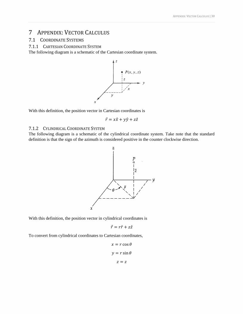
7.1.1 CARTESIAN COORDINATE SYSTEM The following diagram is a schematic of the Cartesian coordinate system.

With this definition, the position vector in Cartesian coordinates is

𝑟 = 𝑥𝑥 + 𝑦�̂� + 𝑧�̂�

7.1.2 CYLINDRICAL COORDINATE SYSTEM The following diagram is a schematic of the cylindrical coordinate system. Take note that the standard

definition is that the sign of the azimuth is considered positive in the counter clockwise direction.

With this definition, the position vector in cylindrical coordinates is

𝑟 = 𝑟�̂� + 𝑧�̂�

To convert from cylindrical coordinates to Cartesian coordinates,

𝑥 = 𝑟 cos 𝜃

𝑦 = 𝑟 sin𝜃

𝑧 = 𝑧


7.1.3 SPHERICAL COORDINATE SYSTEM The following diagram is a schematic of the spherical coordinate system. Note that many mathematics

textbooks use a slightly different convention by swapping the definitions of 𝜃 and 𝜙. Take note that the

standard definition is that the sign of the azimuth is considered positive in the counter clockwise direction

and that the inclination angle is the angle between the zenith direction and a given point.

With this definition, the position vector in spherical coordinates is

𝑟 = 𝑟�̂�

To convert from spherical coordinates to Cartesian coordinates,

𝑥 = 𝑟 sin 𝜃 cos𝜙

𝑦 = 𝑟 sin 𝜃 sin𝜙

𝑧 = 𝑟 cos 𝜃

7.1.4 SURFACE DIFFERENTIALS The surface differentials, 𝑑𝑆, in each of the three major coordinate systems are as follows.

Coordinate system Surface differential, 𝑑𝑆

Cartesian (top, �̂� = �̂�) 𝑑𝑥 𝑑𝑦

Cartesian (side, �̂� = �̂�) 𝑑𝑥 𝑑𝑧 Cartesian (side, �̂� = 𝑥) 𝑑𝑦 𝑑𝑧 Cylindrical (top, �̂� = �̂�) 𝑟 𝑑𝑟 𝑑𝜃

Cylindrical (side, �̂� = �̂�) 𝑟 𝑑𝜃 𝑑𝑧 Spherical (�̂� = �̂�) 𝑟2 sin𝜃 𝑑𝜃 𝑑𝜙

7.1.5 VOLUME DIFFERENTIALS The volume differentials, 𝑑𝑉, in each of the three major coordinate systems are as follows.

Coordinate system Volume differential, 𝑑𝑉

Cartesian 𝑑𝑥 𝑑𝑦 𝑑𝑧 Cylindrical 𝑟 𝑑𝑟 𝑑𝜃 𝑑𝑧 Spherical 𝑟2 sin 𝜃 𝑑𝑟 𝑑𝜃 𝑑𝜙


7.2 MATHEMATICAL OPERATIONS

7.2.1 MAGNITUDE The magnitude of a vector is its length and can be computed as the following.

In the Cartesian coordinate system

|�⃗�| = √𝑣𝑥2 + 𝑣𝑦

2 + 𝑣𝑧2

In the cylindrical coordinate system

|�⃗�| = √𝑣𝑟2 + 𝑣𝑧

2

In the spherical coordinate system

|�⃗�| = 𝑣𝑟

7.2.2 DOT PRODUCT The dot product of two vectors is

�⃗⃗� ⋅ �⃗� = ∑𝑢𝑖𝑣𝑖

𝑛

𝑖=1

The dot product of a tensor with a vector, such as 𝑓 = �̿� ⋅ �⃗⃗� is what one would expect from matrix algebra:

(

𝑓1𝑓2𝑓3

) = (

𝜎𝑖𝑖 𝜎𝑖𝑗 𝜎𝑖𝑘𝜎𝑗𝑖 𝜎𝑗𝑗 𝜎𝑗𝑘𝜎𝑘𝑖 𝜎𝑘𝑗 𝜎𝑘𝑘

) ⋅ (

𝑛1𝑛2𝑛3)

7.2.3 CROSS PRODUCT In matrix notation, the cross product is

�⃗⃗�×�⃗� = det(𝑖̂ 𝑗̂ �̂�𝑢𝑖 𝑢𝑗 𝑢𝑖𝑣𝑖 𝑣𝑗 𝑣𝑗

) = (𝑢𝑗𝑣𝑘 − 𝑢𝑘𝑣𝑗)𝑖̂ + (𝑢𝑘𝑣𝑖 − 𝑢𝑖𝑣𝑘)𝑗̂ + (𝑢𝑖𝑣𝑗 − 𝑢𝑗𝑣𝑖)�̂�

where 𝑖, 𝑗, and 𝑘 represent the three coordinates in the given coordinate system.

7.3 OPERATORS

7.3.1 GRADIENT The gradient is a mathematical operator that acts on a scalar function and is written as grad(𝑓) or ∇𝑓. The

result is always a vector. It is essentially the derivative applied to functions of several variables.

In Cartesian coordinates, the gradient is

ˆ ˆ ˆgrad( )f f f

f x y zx y z


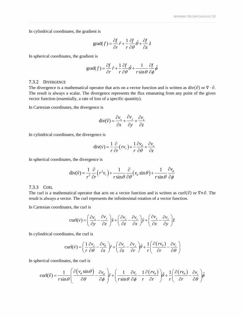
In cylindrical coordinates, the gradient is

1 ˆˆ ˆgrad( )

f f ff r z

r r z

In spherical coordinates, the gradient is

1 1ˆ ˆˆgrad( )sin

f f ff r

r r r

7.3.2 DIVERGENCE The divergence is a mathematical operator that acts on a vector function and is written as div(�⃗�) or ∇ ⋅ �⃗�.

The result is always a scalar. The divergence represents the flux emanating from any point of the given

vector function (essentially, a rate of loss of a specific quantity).

In Cartesian coordinates, the divergence is

div( )yx z

vv vv

x y z

In cylindrical coordinates, the divergence is

1 1

div( ) zr

v vv rv

r r r z

In spherical coordinates, the divergence is

2

2

1 1 1div( ) sin

sin sinr

vv r v v

r r r r

7.3.3 CURL The curl is a mathematical operator that acts on a vector function and is written as curl(�⃗�) or ∇×�⃗�. The

result is always a vector. The curl represents the infinitesimal rotation of a vector function.

In Cartesian coordinates, the curl is

ˆ ˆ ˆcurl( )y yx xz z

v vv vv vv x y z

y z z x x y

In cylindrical coordinates, the curl is

1 1ˆˆcurl( ) z r z rrvvv v v v

v rr z z r r r

In spherical coordinates, the curl is

sin1 1 1 1ˆ ˆˆcurl( )

sin sin

r rv rv rvv v v

v rr r r r r r


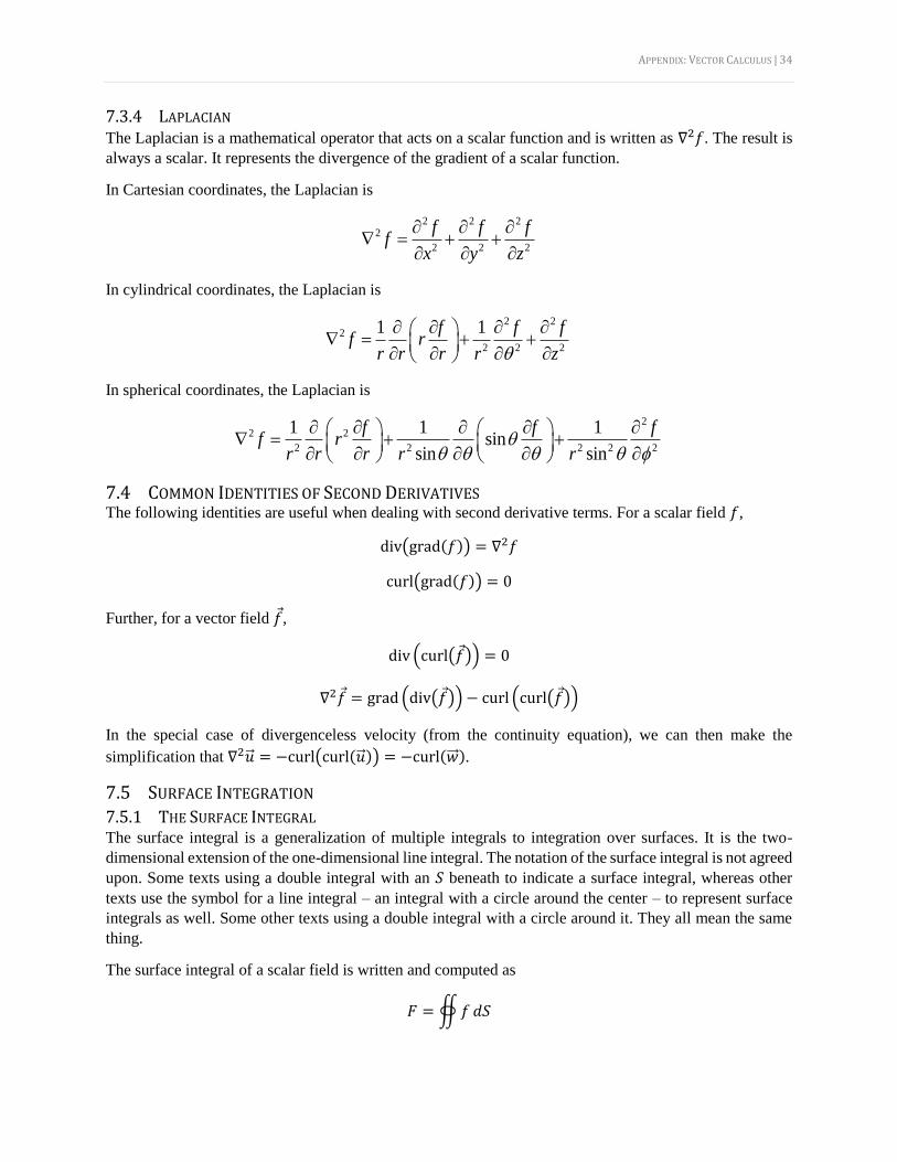
7.3.4 LAPLACIAN The Laplacian is a mathematical operator that acts on a scalar function and is written as ∇2𝑓. The result is

always a scalar. It represents the divergence of the gradient of a scalar function.

In Cartesian coordinates, the Laplacian is

2 2 22

2 2 2

f f ff

x y z

In cylindrical coordinates, the Laplacian is

2 22

2 2 2

1 1f f ff r

r r r r z

In spherical coordinates, the Laplacian is

22 2

2 2 2 2 2

1 1 1sin

sin sin

f f ff r

r r r r r

7.4 COMMON IDENTITIES OF SECOND DERIVATIVES The following identities are useful when dealing with second derivative terms. For a scalar field 𝑓,

div(grad(𝑓)) = ∇2𝑓

curl(grad(𝑓)) = 0

Further, for a vector field 𝑓,

div (curl(𝑓)) = 0

∇2𝑓 = grad (div(𝑓)) − curl (curl(𝑓))

In the special case of divergenceless velocity (from the continuity equation), we can then make the

simplification that ∇2�⃗⃗� = −curl(curl(�⃗⃗�)) = −curl(�⃗⃗⃗�).

7.5 SURFACE INTEGRATION

7.5.1 THE SURFACE INTEGRAL The surface integral is a generalization of multiple integrals to integration over surfaces. It is the two-

dimensional extension of the one-dimensional line integral. The notation of the surface integral is not agreed

upon. Some texts using a double integral with an 𝑆 beneath to indicate a surface integral, whereas other

texts use the symbol for a line integral – an integral with a circle around the center – to represent surface

integrals as well. Some other texts using a double integral with a circle around it. They all mean the same

thing.

The surface integral of a scalar field is written and computed as

𝐹 =∯𝑓 𝑑𝑆


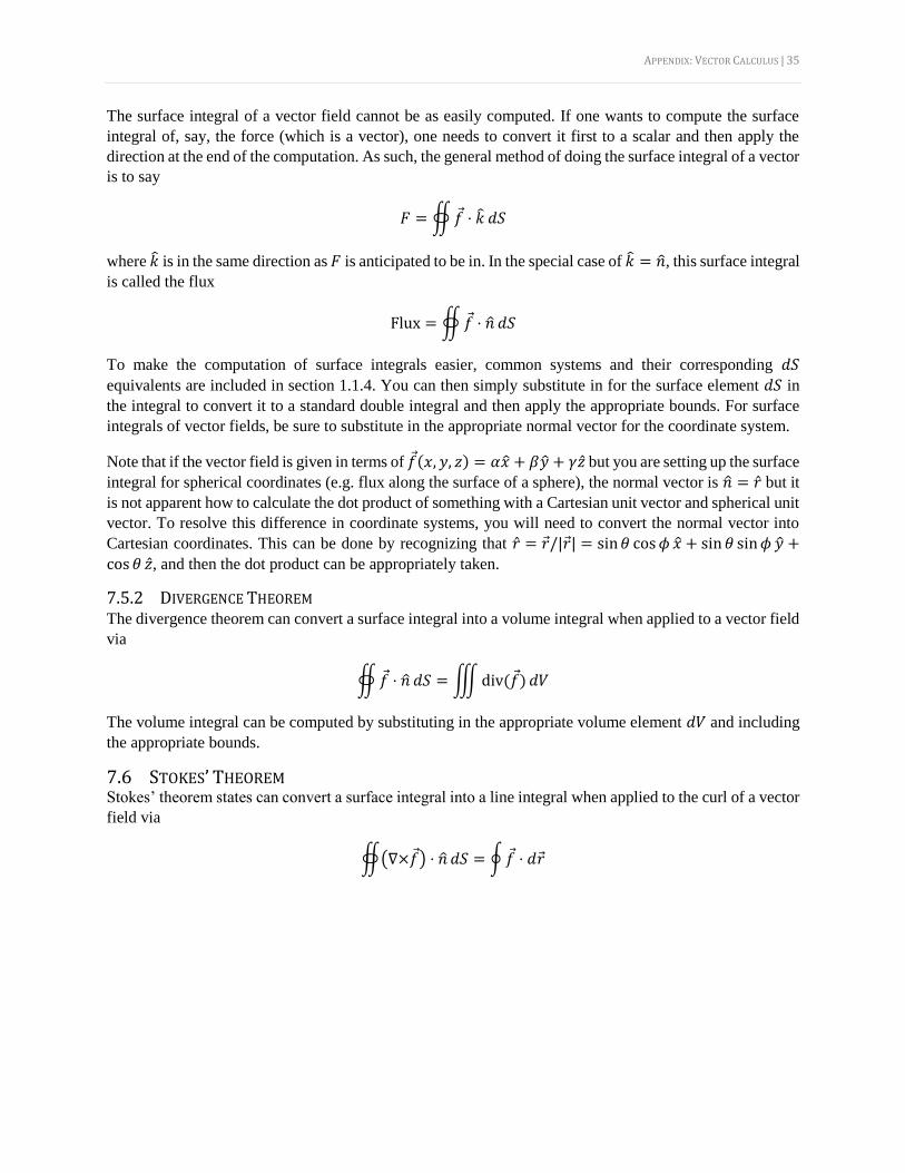
The surface integral of a vector field cannot be as easily computed. If one wants to compute the surface

integral of, say, the force (which is a vector), one needs to convert it first to a scalar and then apply the

direction at the end of the computation. As such, the general method of doing the surface integral of a vector

is to say

𝐹 =∯𝑓 ⋅ �̂� 𝑑𝑆

where �̂� is in the same direction as 𝐹 is anticipated to be in. In the special case of �̂� = �̂�, this surface integral

is called the flux

Flux = ∯𝑓 ⋅ �̂� 𝑑𝑆

To make the computation of surface integrals easier, common systems and their corresponding 𝑑𝑆

equivalents are included in section 1.1.4. You can then simply substitute in for the surface element 𝑑𝑆 in

the integral to convert it to a standard double integral and then apply the appropriate bounds. For surface

integrals of vector fields, be sure to substitute in the appropriate normal vector for the coordinate system.

Note that if the vector field is given in terms of 𝑓(𝑥, 𝑦, 𝑧) = 𝛼𝑥 + 𝛽�̂� + 𝛾�̂� but you are setting up the surface

integral for spherical coordinates (e.g. flux along the surface of a sphere), the normal vector is �̂� = �̂� but it

is not apparent how to calculate the dot product of something with a Cartesian unit vector and spherical unit

vector. To resolve this difference in coordinate systems, you will need to convert the normal vector into

Cartesian coordinates. This can be done by recognizing that �̂� = 𝑟/|𝑟| = sin𝜃 cos𝜙 𝑥 + sin 𝜃 sin𝜙 �̂� +

cos 𝜃 �̂�, and then the dot product can be appropriately taken.

7.5.2 DIVERGENCE THEOREM The divergence theorem can convert a surface integral into a volume integral when applied to a vector field

via

∯𝑓 ⋅ �̂� 𝑑𝑆 =∭div(𝑓) 𝑑𝑉

The volume integral can be computed by substituting in the appropriate volume element 𝑑𝑉 and including

the appropriate bounds.

7.6 STOKES’ THEOREM Stokes’ theorem states can convert a surface integral into a line integral when applied to the curl of a vector

field via

∯(∇×𝑓) ⋅ �̂� 𝑑𝑆 = ∮𝑓 ⋅ 𝑑𝑟

APPENDIX: PRACTICAL PROBLEM SOLVING METHODS | 36

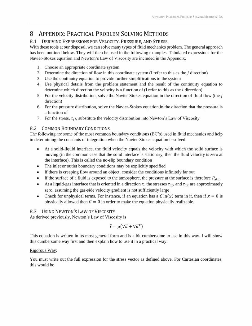
8 APPENDIX: PRACTICAL PROBLEM SOLVING METHODS 8.1 DERIVING EXPRESSIONS FOR VELOCITY, PRESSURE, AND STRESS With these tools at our disposal, we can solve many types of fluid mechanics problem. The general approach

has been outlined below. They will then be used in the following examples. Tabulated expressions for the

Navier-Stokes equation and Newton’s Law of Viscosity are included in the Appendix.

1. Choose an appropriate coordinate system

2. Determine the direction of flow in this coordinate system (I refer to this as the 𝑗 direction)

3. Use the continuity equation to provide further simplifications to the system

4. Use physical details from the problem statement and the result of the continuity equation to

determine which direction the velocity is a function of (I refer to this as the 𝑖 direction)

5. For the velocity distribution, solve the Navier-Stokes equation in the direction of fluid flow (the 𝑗 direction)

6. For the pressure distribution, solve the Navier-Stokes equation in the direction that the pressure is

a function of

7. For the stress, 𝜏𝑖𝑗, substitute the velocity distribution into Newton’s Law of Viscosity

8.2 COMMON BOUNDARY CONDITIONS The following are some of the most common boundary conditions (BC’s) used in fluid mechanics and help

in determining the constants of integration when the Navier-Stokes equation is solved.

At a solid-liquid interface, the fluid velocity equals the velocity with which the solid surface is

moving (in the common case that the solid interface is stationary, then the fluid velocity is zero at

the interface). This is called the no-slip boundary condition

The inlet or outlet boundary conditions may be explicitly specified

If there is creeping flow around an object, consider the conditions infinitely far out

If the surface of a fluid is exposed to the atmosphere, the pressure at the surface is therefore 𝑃atm

At a liquid-gas interface that is oriented in a direction 𝑥, the stresses 𝜏𝑥𝑦 and 𝜏𝑥𝑧 are approximately

zero, assuming the gas-side velocity gradient is not sufficiently large

Check for unphysical terms. For instance, if an equation has a 𝐶 ln(𝑥) term in it, then if 𝑥 = 0 is

physically allowed then 𝐶 = 0 in order to make the equation physically realizable.

8.3 USING NEWTON’S LAW OF VISCOSITY As derived previously, Newton’s Law of Viscosity is

�̿� = 𝜇(∇�⃗⃗� + ∇�⃗⃗�T)

This equation is written in its most general form and is a bit cumbersome to use in this way. I will show

this cumbersome way first and then explain how to use it in a practical way.

Rigorous Way:

You must write out the full expression for the stress vector as defined above. For Cartesian coordinates,

this would be

APPENDIX: PRACTICAL PROBLEM SOLVING METHODS | 37

�̿� = 𝜇

(

(


𝜕𝑢𝑥𝜕𝑦 𝜕𝑢𝑥𝜕𝑧

𝜕𝑢𝑦

𝜕𝑥

𝜕𝑢𝑦

𝜕𝑦

𝜕𝑢𝑦

𝜕𝑧𝜕𝑢𝑧𝜕𝑥 𝜕𝑢𝑧𝜕𝑦


+

(


𝜕𝑢𝑦

𝜕𝑥 𝜕𝑢𝑧𝜕𝑥

𝜕𝑢𝑥𝜕𝑦

𝜕𝑢𝑦

𝜕𝑦

𝜕𝑢𝑧𝜕𝑦

𝜕𝑢𝑥𝜕𝑧 𝜕𝑢𝑦

𝜕𝑧


)

Then, based on the problem, cancel relevant terms that go to zero and you have your expression for the

stress.

Practical Way:

1. Determine what direction the velocity is a function of (I refer to this as the 𝑖 direction)

2. Determine the direction of flow in the coordinate system of choice (I refer to this as the 𝑗 direction)

3. The stress tensor is then written as 𝜏𝑖𝑗 and represents the stress on the positive 𝑖 face acting in the

positive 𝑗 direction3

4. The expression of 𝜏𝑖𝑗 can then be more simply expressed as 𝜏𝑖𝑗 = 𝜇(∇𝑖𝑢𝑗 + ∇𝑗𝑢𝑖). Here, I have

introduced my own short-hand notation. The operator ∇𝑖 represents the gradient operator in the 𝑖

direction and 𝑢𝑗 represents the velocity in the 𝑗 direction. Of course, if there is more than one 𝑖

and/or 𝑗 values (e.g. if the fluid velocity is in greater than one dimension) you will need more than

one expression for 𝜏𝑖𝑗

8.4 CALCULATING MEAN VELOCITY AND FLOW RATE To calculate the mean velocity through a given area, simply divide the total volumetric flow rate by the

cross-sectional area:

⟨𝑢⟩ =∬𝑢 𝑑𝐴

∬𝑑𝐴

using the appropriate 𝑑𝐴 elements for the given coordinate system.

To calculate the volumetric flow rate through a cross-section once the mean velocity is known, this can

typically be found by multiplying the mean velocity in the cross-section by the cross-sectional area. More

generally speaking, the volumetric flow rate can be found by

𝑄 =∬⟨𝑢⟩ 𝑑𝐴

To find the mass flow rate, simply multiply the volumetric flow rate by density.

3 Note that many textbooks, most notably BSL, define the stress tensor differently with a negative sign in the front.

APPENDIX: TABULATED EXPRESSIONS | 38

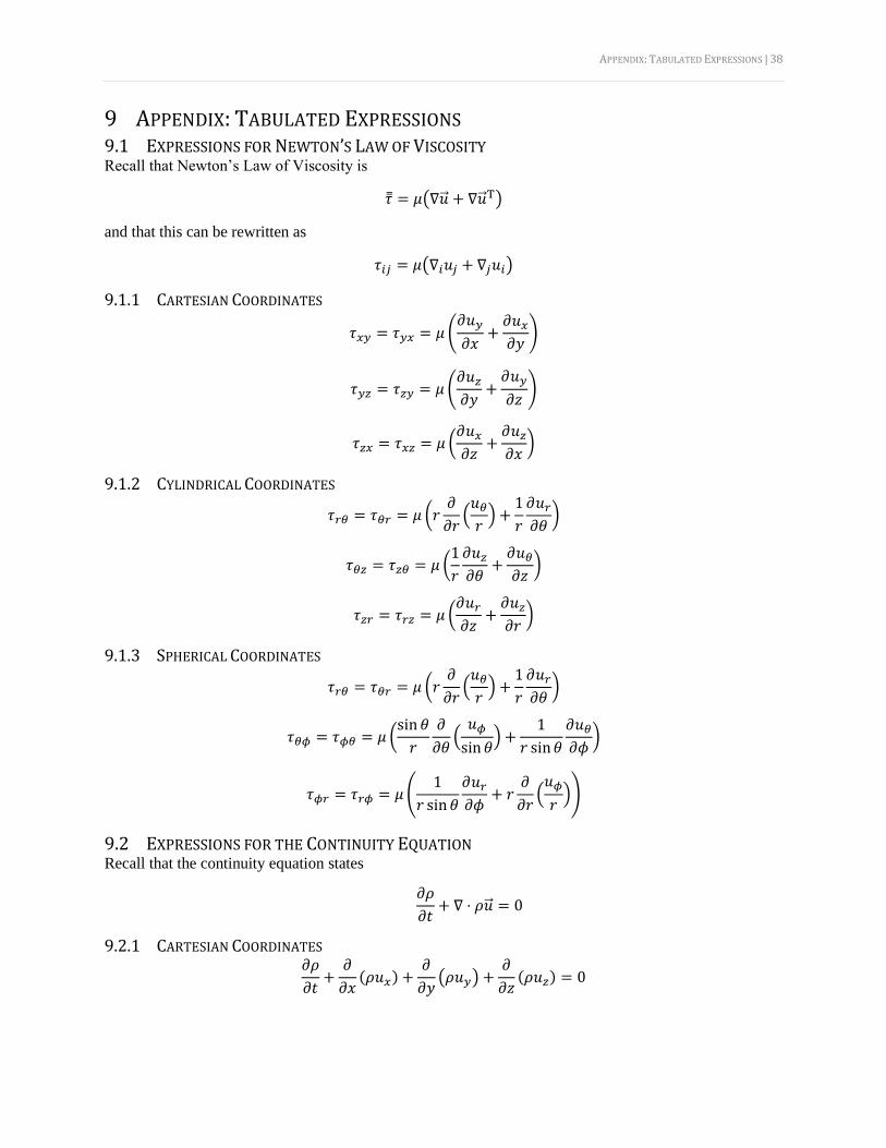
9 APPENDIX: TABULATED EXPRESSIONS 9.1 EXPRESSIONS FOR NEWTON’S LAW OF VISCOSITY Recall that Newton’s Law of Viscosity is

�̿� = 𝜇(∇�⃗⃗� + ∇�⃗⃗�T)

and that this can be rewritten as

𝜏𝑖𝑗 = 𝜇(∇𝑖𝑢𝑗 + ∇𝑗𝑢𝑖)

9.1.1 CARTESIAN COORDINATES

𝜏𝑥𝑦 = 𝜏𝑦𝑥 = 𝜇 (𝜕𝑢𝑦

𝜕𝑥+𝜕𝑢𝑥𝜕𝑦)

𝜏𝑦𝑧 = 𝜏𝑧𝑦 = 𝜇 (𝜕𝑢𝑧𝜕𝑦

+𝜕𝑢𝑦

𝜕𝑧)

𝜏𝑧𝑥 = 𝜏𝑥𝑧 = 𝜇 (𝜕𝑢𝑥𝜕𝑧

+𝜕𝑢𝑧𝜕𝑥)

9.1.2 CYLINDRICAL COORDINATES

𝜏𝑟𝜃 = 𝜏𝜃𝑟 = 𝜇 (𝑟𝜕


1

𝑟


𝜏𝜃𝑧 = 𝜏𝑧𝜃 = 𝜇 (1

𝑟

𝜕𝑢𝑧𝜕𝜃

+𝜕𝑢𝜃𝜕𝑧)

𝜏𝑧𝑟 = 𝜏𝑟𝑧 = 𝜇 (𝜕𝑢𝑟𝜕𝑧

+𝜕𝑢𝑧𝜕𝑟)

9.1.3 SPHERICAL COORDINATES

𝜏𝑟𝜃 = 𝜏𝜃𝑟 = 𝜇 (𝑟𝜕


1

𝑟


𝜏𝜃𝜙 = 𝜏𝜙𝜃 = 𝜇 (sin 𝜃

𝑟

𝜕

𝜕𝜃(𝑢𝜙

sin 𝜃) +

1

𝑟 sin𝜃

𝜕𝑢𝜃𝜕𝜙)

𝜏𝜙𝑟 = 𝜏𝑟𝜙 = 𝜇 (1

𝑟 sin 𝜃

𝜕𝑢𝑟𝜕𝜙

+ 𝑟𝜕

𝜕𝑟(𝑢𝜙

𝑟))

9.2 EXPRESSIONS FOR THE CONTINUITY EQUATION Recall that the continuity equation states

𝜕𝜌

𝜕𝑡+ ∇ ⋅ 𝜌�⃗⃗� = 0

9.2.1 CARTESIAN COORDINATES 𝜕𝜌

𝜕𝑡+𝜕

𝜕𝑥(𝜌𝑢𝑥) +

𝜕

𝜕𝑦(𝜌𝑢𝑦) +

𝜕

𝜕𝑧(𝜌𝑢𝑧) = 0

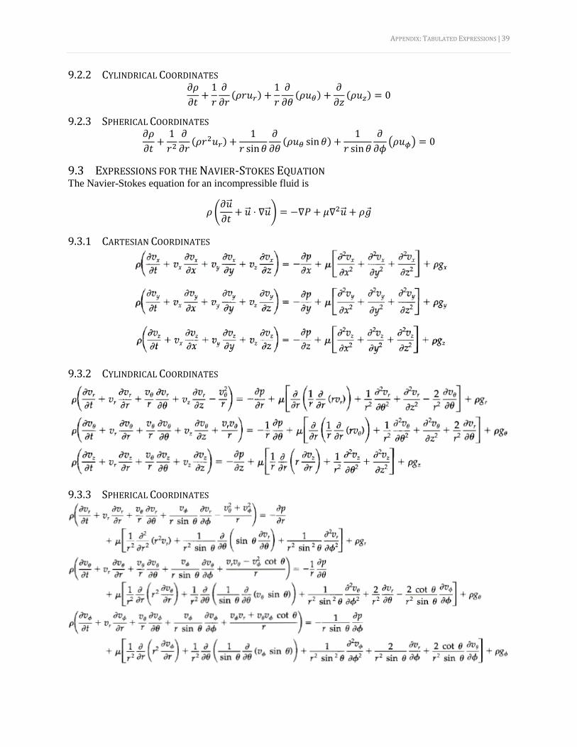
APPENDIX: TABULATED EXPRESSIONS | 39

9.2.2 CYLINDRICAL COORDINATES 𝜕𝜌

𝜕𝑡+1

𝑟

𝜕

𝜕𝑟(𝜌𝑟𝑢𝑟) +

1

𝑟

𝜕

𝜕𝜃(𝜌𝑢𝜃) +

𝜕

𝜕𝑧(𝜌𝑢𝑧) = 0

9.2.3 SPHERICAL COORDINATES 𝜕𝜌

𝜕𝑡+1

𝑟2𝜕

𝜕𝑟(𝜌𝑟2𝑢𝑟) +

1

𝑟 sin𝜃

𝜕

𝜕𝜃(𝜌𝑢𝜃 sin 𝜃) +

1

𝑟 sin𝜃

𝜕

𝜕𝜙(𝜌𝑢𝜙) = 0

9.3 EXPRESSIONS FOR THE NAVIER-STOKES EQUATION The Navier-Stokes equation for an incompressible fluid is

𝜌 (𝜕�⃗⃗�

𝜕𝑡+ �⃗⃗� ⋅ ∇�⃗⃗�) = −∇𝑃 + 𝜇∇2�⃗⃗� + 𝜌�⃗�

9.3.1 CARTESIAN COORDINATES

9.3.2 CYLINDRICAL COORDINATES

9.3.3 SPHERICAL COORDINATES

fluid mechanics - tufts university kinds of forces are typically considered in the study of fluid...

Documents