fluid flow and heat transfer in a dual-wet micro heat pipe

Zhang, J. and Watson, S.J. and Wong, H. (2007) Fluid flow and heat transfer in a dual-wet micro heat pipe. Journal of Fluid Mechanics, 589 . pp. 1-31. ISSN 0022-1120

http://eprints.gla.ac.uk/25358/ Deposited on: 27 April 2010

Enlighten – Research publications by members of the University of Glasgow http://eprints.gla.ac.uk

J. Fluid Mech. (2007), vol. 589, pp. 1–31. c© 2007 Cambridge University Press

doi:10.1017/S0022112007007823 Printed in the United Kingdom

1

Fluid flow and heat transfer in a dual-wetmicro heat pipe

JIN ZHANG1, STEPHEN J. WATSON2 AND HARRIS WONG1†1Department of Mechanical Engineering, Louisiana State University, Baton Rouge,

LA 70803-6413, USA2Department of Mathematics, Louisiana State University, Baton Rouge, LA 70803-6413, USA

(Received 6 May 2006 and in revised form 16 May 2007)

Micro heat pipes have been used to cool micro electronic devices, but their heattransfer coefficients are low compared with those of conventional heat pipes. In thiswork, a dual-wet pipe is proposed as a model to study heat transfer in micro heatpipes. The dual-wet pipe has a long and narrow cavity of rectangular cross-section.The bottom-half of the horizontal pipe is made of a wetting material, and the top-halfof a non-wetting material. A wetting liquid fills the bottom half of the cavity, whileits vapour fills the rest. This configuration ensures that the liquid–vapour interfaceis pinned at the contact line. As one end of the pipe is heated, the liquid evaporatesand increases the vapour pressure. The higher pressure drives the vapour to the coldend where the vapour condenses and releases the latent heat. The condensate movesalong the bottom half of the pipe back to the hot end to complete the cycle. We solvethe steady-flow problem assuming a small imposed temperature difference betweenthe two ends of the pipe. This leads to skew-symmetric fluid flow and temperaturedistribution along the pipe so that we only need to focus on the evaporative half ofthe pipe. Since the pipe is slender, the axial flow gradients are much smaller than thecross-stream gradients. Thus, we can treat the evaporative flow in a cross-sectionalplane as two-dimensional. This evaporative motion is governed by two dimensionlessparameters: an evaporation number E defined as the ratio of the evaporative heatflux at the interface to the conductive heat flux in the liquid, and a Marangoni numberM . The motion is solved in the limit E → ∞ and M → ∞. It is found that evaporationoccurs mainly near the contact line in a small region of size E−1W , where W is the half-width of the pipe. The non-dimensional evaporation rate Q∗ ∼ E−1 ln E as determinedby matched asymptotic expansions. We use this result to derive analytical solutionsfor the temperature distribution Tp and vapour and liquid flows along the pipe. Thesolutions depend on three dimensionless parameters: the heat-pipe number H , whichis the ratio of heat transfer by vapour flow to that by conduction in the pipe walland liquid, the ratio R of viscous resistance of vapour flow to interfacial evaporationresistance, and the aspect ratio S. If HR � 1, a thermal boundary layer appears nearthe pipe end, the width of which scales as (HR)−1/2L, where L is the half-lengthof the pipe. A similar boundary layer exists at the cold end. Outside the boundarylayers, Tp varies linearly with a gradual slope. Thus, these regions correspond to theevaporative, adiabatic and condensing regions commonly observed in conventionalheat pipes. This is the first time that the distinct regions have been captured bya single solution, without prior assumptions of their existence. If HR ∼ 1 or less,then Tp is linear almost everywhere. This is the case found in most micro-heat-pipe

† Author to whom correspondence should be addressed: [email protected].

2 J. Zhang, S. J. Watson and H. Wong

experiments. Our analysis of the dual-wet pipe provides an explanation for thecomparatively low effective thermal conductivity in micro heat pipes, and points toways of improving their heat transfer capabilities.

1. IntroductionA conventional heat pipe is a closed duct filled with a liquid and its vapour. The

duct is usually circular in cross-section with the inner wall covered by a layer of porousmaterial (Peterson 1994; Faghri 1995). The liquid fills the porous lining whereas thevapour fills the rest. As one end of a heat pipe is heated, the liquid evaporatesand increases the vapour pressure. The higher pressure drives the vapour to thecold end, where the vapour condenses and releases the latent heat. The condensatethen flows along the porous lining back to the hot end to complete the cycle. Heatpipes are efficient in transferring heat because thermal energy is carried from oneend to another by evaporation, convection and condensation. Their effective thermalconductivity can be 30 times that of copper (Peterson 1994). Furthermore, there isno moving mechanical machinery in a heat pipe, resulting in low maintenance andoperating costs. Consequently, heat pipes have been installed in the thermal controlof, for example, the Alaska pipeline, nuclear reactor cores, and the leading edge ofhypersonic aircraft (Peterson 1994; Faghri 1995).

Micro heat pipes have been developed to control the temperature of micro electronicdevices (Groll et al. 1998; Sobhan, Rag & Peterson 2007). A micro heat pipe is along polygonal (e.g. triangular or rectangular) capillary filled with a liquid and along vapour bubble. The length of the bubble is comparable to that of the capillary.Figure 1 shows a vapour bubble in a square capillary under uniform temperature(Wong, Radke & Morris 1995). A cross-section reveals that the corners are occupiedby liquid menisci. These channels allow liquid to flow from the cold to the hot end,functioning as the porous lining in a conventional heat pipe.

The operation of a micro heat pipe is similar to that of the conventional heatpipe. As one end of a micro heat pipe is heated, the liquid evaporates and the cornermenisci recede into the corners. The higher vapour pressure at the hot end drivesthe vapour to the cold end where it condenses and releases the latent heat. Thecondensate then flows along the corner channels back to the hot end to completethe cycle. The corner flow is driven by an axial capillary-pressure gradient. A microheat pipe can be as small as 50 µm in width, and it can be fabricated as part ofan electronic circuitry. As a result, micro heat pipes are especially suited for thermalcontrol of micro electronic devices (Groll et al. 1998).

The steady operation of a micro heat pipe was first modelled by Cotter (1984), whoassumed liquid and vapour flows to be unidirectional. This allows the local pressuregradient to be related to the local mass flow rate. Under steady operation, the vapourand liquid mass flow rates must be equal and opposite at each point along the pipe.The vapour flow carries the latent heat and is proportional to the local heat flux(assumed known). The pressure jump across the interface is equated to the capillarypressure. This yields a differential equation for the radius of curvature of the interfacein terms of the known heat flux. Solution of the equation leads to an estimate of themaximum heat flux through the pipe. The predicted maximum heat flow is more thandouble the values measured in experiments, and the model has been modified to yieldbetter agreement with experiments (Longtin, Badran & Gerner 1994; Ha & Peterson

Fluid flow and heat transfer in a dual-wet micro heat pipe 3

Figure 1. Half of a square micro heat pipe under uniform temperature. The liquid-filledcorners provide a channel for liquid flow.

1998). This approach does not use the energy equation and therefore cannot describethe temperature distribution along the pipe.

Khrustalev & Faghri (1994) developed a more comprehensive model that includesthe energy equation. They separated the pipe into three distinct regions (evaporator,adiabatic and condenser), and treated each region differently. In the evaporatorregion, they considered the meniscus near the contact line and incorporated previouslypublished results on evaporation due to superheat and disjoining pressure (Wu &Wong 2004). In the condenser region, they assumed that a liquid film covers the walland found the film profile based on the latent heat released by the condensate. Inthe adiabatic region, they imposed the condition that the liquid flow rate is constant.They then connected the three regions together by appropriate continuity conditions.Their model neglects axial heat conduction in the wall and liquid, and focuses insteadon the vapour temperature. When their model is applied to the experiments by Wu &Peterson (1991), good agreement is obtained for the maximum heat flow. A similarapproach is adopted by Launay, Sartre & Lallemand (2004) to calculate the effectivethermal conductivity as a function of the liquid fill charge.

Suman & Kumar (2005) considered axial heat conduction in the pipe wall. Theyalso separated the pipe into three regions, but they neglected the evaporation andcondensation kinetics. Instead, the vapour flow rate is related to the heat flux,which is equated to the conductive heat flux along the pipe wall. Patching the threeregions allows them to find the axial temperature distribution in the pipe. Here, westudy in detail the evaporation and condensation mechanisms, and find an analyticsolution for the pipe temperature that contains the three distinct regions withoutprior assumptions of their existence.

The effective thermal conductivity of micro heat pipes is far below that ofconventional heat pipes. A typical value for the effective thermal conductivity of aconventional heat pipe is 13 200 Wm−1 K−1 (Peterson 1994), whereas that of a microheat pipe is 300 Wm−1 K−1 (Peterson, Duncan & Weichold 1993; Badran et al. 1997).The effective thermal conductivity of a micro heat pipe with and without a liquiddiffers by at most 50% (Peterson et al. 1993; Badran et al. 1997). The experimentalstudy by Le Berre et al. (2003) uses a triangular micro channel with an attached sidechannel for liquid flow. They were able to obtain an effective thermal conductivity of600 Wm−1 K−1. A conventional heat pipe has three distinct temperature regions alongthe pipe: evaporative, adiabatic and condensing. The temperature is almost uniformin the middle adiabatic section, which is the main reason for the large effectivethermal conductivity. However, this adiabatic region is missing in most micro heatpipes (Badran et al. 1997; Le Berre et al. 2003). Thus, it seems that the heat transfercapability of micro heat pipes has not been fully developed.


2W

2W

2W

z

L

xy

Figure 2. Heated half of a dual-wet heat pipe. The bottom half of the pipe is made of awetting material and is filled by a wetting liquid, whereas the top half, which is made of anon-wetting material, is occupied by the vapour. This ensures that the contact line of theliquid-vapour interface is pinned. A coordinate system (x, y, z) is defined at the middle of thepipe with z pointing towards the hot end. The width of the pipe is 2W .

To understand the basic heat transfer mechanisms of micro heat pipes, it is better toanalyse a system without the complicated bubble geometry, but with all the essentialphysics retained. There are several basic elements of micro heat pipes that are requiredfor heat transfer. The corner menisci serve as a channel for liquid flow. Thus, the newsystem must also contain a liquid flow channel. The liquid–vapour interfaces at thehot and cold ends change their curvatures owing to evaporation and condensation.Thus, the new system must also include a liquid–vapour interface that separates thevapour and liquid flow channels, and the interface must be able to deform underevaporation and condensation. The deformation must occur in such a way as togenerate a capillary pressure difference that drives the liquid from the cold end to thehot end. Finally, the contact line has been shown to play a crucial role in evaporationand condensation and must be retained in the new system. Below, a dual-wet microheat pipe is proposed which captures all these essential elements.

1.1. A dual-wet micro heat pipe

Figure 2 shows our proposed micro heat pipe, the bottom portion of which is madeof a wetting material, while the top portion is a non-wetting material. The wettingportion is filled to the rim by a wetting liquid, and the non-wetting portion is filledby its vapour. This configuration ensures that the contact line of the liquid–vapourinterface is pinned at the transition point between the wetting and the non-wettingwall material (Gau et al. 1999; Darhuber, Troian & Reisner 2001). Pinning of theinterface allows a capillary-pressure gradient to drive the liquid flow. When thismicro heat pipe is driven at a small temperature difference, the interface should beapproximately flat, allowing the analysis to be greatly simplified. The goal of studyingthis dual-wet micro heat pipe is to identify key parameters that govern heat transfer.

The heat transfer mechanism of a micro heat pipe can be understood as follows.Initially, the pipe is at a uniform temperature T0. One end of the heat pipe is thenheated to temperature T0 + �T , and the other end cooled to T0 − �T . The temperaturedifference is maintained and the heat pipe reaches a steady state. At the hot end,the equilibrium vapour pressure is higher than that at the cold end, and the vapour-pressure gradient drives a vapour flow. Because the vapour moves away from the hot


end, the vapour pressure at the hot end drops below the equilibrium value, and thispressure drop induces continuous evaporation. At the cold end, the vapour pressureis higher than the local equilibrium vapour pressure, leading to condensation. Thecondensate increases the liquid volume at the cold end and raises the liquid–vapourinterface, whereas the interface sags at the hot end owing to evaporation. Because thecontact lines are pinned, the interfacial profile creates a capillary pressure gradientin the liquid along the pipe, which drives the liquid from the cold to the hot end. Ingeneral, �T � T0, and the vapour and liquid flows and the temperature distributionalong the pipe are skew-symmetric about the midpoint of the pipe. Thus, only theheated half of the pipe is studied (figure 2).

Flow fields inside a micro heat pipe vary slowly in the axial direction because ofthe high aspect ratio of the pipe. Hence, at each cross-sectional plane, the evaporativemotion can be taken as two-dimensional. This in-plane motion is studied first;the governing equations are given in § 2 and are made dimensionless in § 3. Twodimensionless parameters emerge: an evaporation number E (�1) and a Marangoninumber M (�1). The evaporation number E measures the ratio of the evaporativeheat flux at the interface to the conductive heat flux in the liquid, if both are drivenby the same temperature difference. The temperature field in the cross-sectional planedepends on E only, and is solved in the limit E → ∞ in § 4. The temperature fieldhas a singular region near the contact line and is resolved by the method of matchedasymptotic expansions. This leads to an analytical expression for the interfacialtemperature, which is used to find the evaporation rate Q in the cross-sectional planein § 5. The liquid flow in the cross-sectional plane does not affect the evaporation rateand is presented in the Appendix.

Sections 6 to 10 use Q to find the temperature distribution and vapour and liquidflows along the pipe. The heat rate q is constant along the pipe because the pipe isinsulated at the outer wall. Inside the pipe, heat is transferred by vapour flow and byconduction in the liquid and wall, and the sum is equal to q , as shown in § 6. The twomodes of heat transfer are coupled by the local evaporation rate Q found in § 5. Theevaporation rate Q depends on the local vapour pressure pg and pipe temperatureTp . This is a unique feature of our model, and it leads to a thermal boundary layernear the pipe end.

The pipe temperature Tp is solved in § 7. The analytic solution depends on threedimensionless numbers: H, R and the aspect ratio S (=W/L) of the pipe. The Heat-pipe number H is the ratio of heat transfer by vapour flow to that by conductionin the pipe wall and liquid, whereas R is the ratio of viscous resistance of vapourflow to interfacial evaporation resistance for the same pressure gradient and volumeflow rate. If HR � 1, a thermal boundary layer appears near the pipe end in whichthe temperature varies rapidly. The width of the layer scales as (HR)−1/2L, where L

is half the pipe length. Outside the boundary layer, the temperature varies linearlywith a small slope. Thus, these regions correspond to the evaporative, adiabatic andcondensing regions commonly observed in heat pipes. This is the first time thatthe distinct regions are captured by a single temperature distribution, without priorassumptions of their existence. If HR ∼ 1 or less, then the temperature field is almostlinear. This is the case found in most micro-heat-pipe experiments. Our analysis of thedual-wet micro heat pipe provides an explanation for the lack of three distinct regions,and for the comparatively low effective thermal conductivity in micro heat pipes.

The constant heat rate q through the pipe is also determined in § 7. The conductiveheat rate qc is used to make q dimensionless and this yields a Nusselt numberNu = q/qc. We find that as H → ∞, Nu ∼ H , and as H → 0, Nu → 1.


Vapour

Liquid

x

yTpTp

W = 1 W = 1

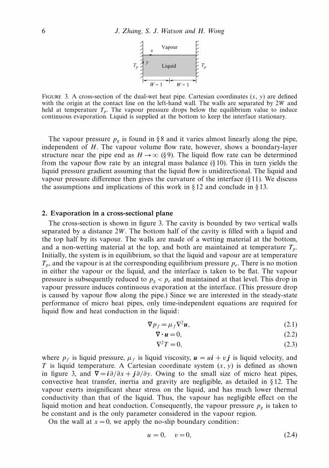
Figure 3. A cross-section of the dual-wet heat pipe. Cartesian coordinates (x, y) are definedwith the origin at the contact line on the left-hand wall. The walls are separated by 2W andheld at temperature Tp . The vapour pressure drops below the equilibrium value to inducecontinuous evaporation. Liquid is supplied at the bottom to keep the interface stationary.

The vapour pressure pg is found in § 8 and it varies almost linearly along the pipe,independent of H . The vapour volume flow rate, however, shows a boundary-layerstructure near the pipe end as H → ∞ (§ 9). The liquid flow rate can be determinedfrom the vapour flow rate by an integral mass balance (§ 10). This in turn yields theliquid pressure gradient assuming that the liquid flow is unidirectional. The liquid andvapour pressure difference then gives the curvature of the interface (§ 11). We discussthe assumptions and implications of this work in § 12 and conclude in § 13.

2. Evaporation in a cross-sectional planeThe cross-section is shown in figure 3. The cavity is bounded by two vertical walls

separated by a distance 2W . The bottom half of the cavity is filled with a liquid andthe top half by its vapour. The walls are made of a wetting material at the bottom,and a non-wetting material at the top, and both are maintained at temperature Tp .Initially, the system is in equilibrium, so that the liquid and vapour are at temperatureTp , and the vapour is at the corresponding equilibrium pressure pe. There is no motionin either the vapour or the liquid, and the interface is taken to be flat. The vapourpressure is subsequently reduced to pg <pe and maintained at that level. This drop invapour pressure induces continuous evaporation at the interface. (This pressure dropis caused by vapour flow along the pipe.) Since we are interested in the steady-stateperformance of micro heat pipes, only time-independent equations are required forliquid flow and heat conduction in the liquid:

∇pf = µf ∇2u, (2.1)

∇ · u = 0, (2.2)

∇2T = 0, (2.3)

where pf is liquid pressure, µf is liquid viscosity, u = ui + v j is liquid velocity, andT is liquid temperature. A Cartesian coordinate system (x, y) is defined as shownin figure 3, and ∇ = i∂/∂x + j∂/∂y. Owing to the small size of micro heat pipes,convective heat transfer, inertia and gravity are negligible, as detailed in § 12. Thevapour exerts insignificant shear stress on the liquid, and has much lower thermalconductivity than that of the liquid. Thus, the vapour has negligible effect on theliquid motion and heat conduction. Consequently, the vapour pressure pg is taken tobe constant and is the only parameter considered in the vapour region.

On the wall at x = 0, we apply the no-slip boundary condition:

u = 0, v =0, (2.4)


and impose a prescribed constant temperature,

T = Tp. (2.5)

Owing to symmetry, only half of the cross-sectional domain need be analysed. Atthe symmetry plane x =W ,

∂v

∂x= 0, u =0,

∂T

∂x= 0. (2.6)

The interface is pinned at the walls between the wetting and non-wetting parts, andliquid is replenished at the bottom to balance the loss by evaporation. The interface istaken as flat because surface tension dominates in micro heat pipes owing to the smallsize. Thus, the interface is located at y = 0 (figure 3). At the interface, the verticalvelocity v is non-zero owing to evaporation:

m = −ρf v, (2.7)

where ρf is the liquid density and m is the local evaporative mass flux (m is positivefor evaporation and negative for condensation). The evaporation rate in half of thedomain is

Q =

∫ W

0

v dx. (2.8)

The main purpose of the two-dimensional analysis in the cross-sectional plane is tofind Q. At the interface, the evaporative heat flux is supplied by the conductive heatflux in the liquid:

mhfg = kf

∂T

∂y. (2.9)

Here, hfg is the latent heat of evaporation, and kf is the liquid thermal conductivity.The interfacial shear stress in the liquid balances a surface tension gradient:

µf

∂u

∂y= −dσ

dx= − dσ

dT

dT

dx, (2.10)

where σ is the surface tension, which varies along the interface because the tem-perature varies. In this work, dσ/dT is assumed constant owing to the small variationin temperature. The normal stress balance does not enter at this stage since theinterface is taken as flat.

The evaporative mass flux is assumed to be proportional to the drop in vapourpressure from the equilibrium value (Plesset & Prosperetti 1976; Wayner 1993;Ajaev & Homsy 2006):

m = c(pi − pg), c =α

(2πRsTp)1/2, (2.11)

where pi is the equilibrium vapour pressure at the local interfacial temperatureTi = Ti(x), α is the accommodation coefficient, and Rs is the specific gas constant.The parameter c is proportional to the inverse of the sound speed in vapour. Theflux equation (2.11), derived by a kinetic theory, conserves momentum and energy atthe interface, whereas some other commonly used forms do not (Barrett & Clement1992). We can express pi in terms of Ti . Since pi is only a function of the interfacialtemperature Ti and pi is close to pg , by Taylor’s expansion,

pi = pg +dpi

dTi

(Ti − Tg) (2.12)


where Tg is the liquid–vapour equilibrium temperature at pressure pg . The gradientdpi/dTi can be evaluated using the Clapeyron relation because pi = pi(Ti) is athermodynamic relation (Carey 1992):

dpi

dTi

=ρehfg

Tp

, (2.13)

where ρe is the equilibrium vapour density at temperature Tp . Although the gradientshould be evaluated at temperature Tg , we use Tp because it is a boundary conditionand because |Tp − Tg| � Tp and only the linear term in temperature is kept in (2.12).Substitution of pi in (2.12) into (2.11) yields

m =cρehfg(Ti − Tg)

Tp

, (2.14)

therefore, the evaporative mass flux m =m(Ti). This equation is similar to that usedby Burelbach, Bankoff & Davis (1988).

Far below the pinned interface, the liquid flow is non-zero owing to evaporationand the temperature approaches the wall temperature. Thus, as y → ∞,∫ W

0

v dx → −Q, u → 0, T → Tp. (2.15)

Here, we have modified the liquid domain so that the bottom wall is extended toinfinity. This modification allows a simple analytic solution for the temperature fieldand has a negligible effect on the evaporation rate Q, as shown in § 5 (see also § 12).

3. Dimensionless equations governing evaporationSince the liquid motion is induced by evaporation, the surface evaporative flux

equation (2.7), (2.11) and (2.14) are used to yield a velocity scale:

U =c

ρf

(pe − pg) =cρehfg(Tp − Tg)

ρf Tp

. (3.1)

A set of dimensionless variables is defined:

x∗ =x

W, y∗ =

y

W, u∗ =

u

U, p∗

f =pf W

µf U, T ∗ =

T − Tg

Tp − Tg

, Q∗ =Q

UW. (3.2)

The governing equations become

∇∗p∗f = ∇∗2u∗, (3.3)

∇∗ · u∗ =0, (3.4)

∇∗2T ∗ = 0, (3.5)

where ∇∗ = i∂/∂x∗ + j∂/∂y∗. At the wall x∗ = 0,

u∗ = 0, v∗ =0, T ∗ = 1. (3.6)

At the symmetric plane x∗ = 1,

∂v∗

∂x∗ = 0, u∗ = 0,∂T ∗

∂x∗ = 0. (3.7)

At the interface y∗ = 0,

v∗ = −T ∗,∂u∗

∂y∗ = M∂T ∗

∂x∗ , ET ∗ =dT ∗

dy∗ , (3.8)


in which

M = − ρf Tp

cρehfgµf

dσ

dT, E =

cWρeh2fg

kf Tp

. (3.9)

Here, M is the Marangoni number, which measures the ratio of the surface tensiongradient induced by temperature variation to the viscous shear stress caused byevaporation at the interface (Levich 1962). We define an evaporation number E thatreflects the ratio of the evaporative heat flux at the interface to the conductive heatflux in the liquid, assuming that both are driven by the same temperature difference.It identifies a length scale (E−1W ) over which the conductive heat flux becomescomparable to the evaporative heat flux under the same temperature difference. Theevaporation number E is the inverse of the non-equilibrium parameter defined byBurelbach et al. (1988). For a silicon micro heat pipe 45 µm wide charged withmethanol at 42 ◦C, M = 40.8 and E = 780 (Peterson et al. 1993). (The parameters aregiven in table 1)

Far from the liquid interface as y∗ → ∞,∫ 1

0

v∗ dx∗ → −Q∗, u∗ → 0, T ∗ → 1. (3.10)

The dimensionless evaporation rate in half the domain is found from the verticalliquid velocity at the interface:

Q∗ = −∫ 1

0

v∗ dx∗. (3.11)

Since v∗ = −T ∗ at the interface as specified by (3.8),

Q∗ =

∫ 1

0

T ∗ dx∗. (3.12)

Thus, to find Q∗, we need only to focus on the interfacial temperature.The above fluid flow and heat transfer problem contains two dimensionless

parameters: E(�1) and M(�1). The temperature field depends only on E. Thevelocity field is coupled to the temperature field through the boundary conditions,in which M appears. Since the objective of the two-dimensional analysis is to findQ∗, which depends only on the interfacial temperature, we will focus below on thetemperature field and present the velocity solution in the Appendix.

4. Temperature field in the cross-sectional planeThe temperature field is expanded in the limit E → ∞ as

T ∗ = t0 +E−1t1 + · · · . (4.1)

A boundary layer exists near the wall. This is shown by a discontinuity in the leading-order temperature field t0. To see the discontinuity, T ∗ in (4.1) is substituted into (3.6)to yield t0 = 1 at the wall x∗ = 0. However, substitution of T ∗ in (4.1) into (3.8) leadsto t0 = 0 at y∗ = 0. This jump in temperature at the contact line appears often inevaporation problems and leads to unbounded temperature gradients. In the presentproblem, this jump results from the disappearance of the derivative in (3.8) because itis multiplied by E−1. This hints at the existence of an inner region. An inner problemis formulated next which shows that the temperature T ∗ decays smoothly along theinterface from T ∗ = 1 at the wall to T ∗ = 0 away from the wall in a distance scaled by


1.0

0.8

0.6

0.4

0.2

0 5 10X

15 20

τ

Figure 4. Dimensionless temperature τ along the liquid–vapour interface in the inner regionas given by (4.4).

E−1. The existence of the inner problem results from the constitutive equation (2.14)for the evaporative mass flux, and from the constant temperature condition at thewall.

4.1. Inner temperature τ

A set of inner variables is defined as

X = Ex∗, Y = Ey∗, τ (X, Y ) = T ∗(x∗, y∗). (4.2)

The inner temperature field obeys

∇2τ = 0. (4.3a)

At the wall X = 0,

τ = 1. (4.3b)

At the liquid–vapour interface Y= 0,

τ =∂τ

∂Y. (4.3c)

As X → ∞,

τ → 0. (4.3d)

Since the parameter E is scaled out of the problem, this inner solution holds for all or-ders of E. Thus, the inner problem describes the local behaviour near the contact line.It is intrinsic to the evaporation problem, and is independent of the outer problem.

To solve (4.3), a new dependent variable is defined: G = ∂τ/∂Y − τ (Morris 2000).The governing equation remains the same, ∇2G = 0, but the boundary condition atthe liquid–vapour interface Y = 0 is reduced to G = 0, and that at the wall X =0,G = −1. This leads to a simple solution: G =(2/π)tan−1 (X/Y ) − 1. Thus, the innertemperature obeys ∂τ/∂Y − τ = (2/π) tan−1(X/Y ) − 1, the solution of which is

τ =1 − 2

πtan−1

(X

Y

)+

2

πeY X

∫ ∞

Y

e−λ

λ2 + X2dλ. (4.4)

The temperature distribution along the liquid–vapour interface is plotted in figure 4.It indicates that the temperature varies smoothly from 1 at the wall to 0 away fromthe wall. This solution agrees with that of Morris (2000) who considered a more


general problem in which the isothermal condition is not imposed at the solid–liquidinterface, but at the outer wall of the solid. Also, in his problem, the liquid–vapourinterface need not be perpendicular to the wall. These additional complexities onlychange the total evaporation rate by a factor that is less than or equal to one.

4.2. Zero-order outer temperature t0

According to the expansion in (4.1), the zero-order outer temperature satisfies

∇2t0 = 0. (4.5a)

At the wall x∗ = 0,

t0 = 1, (4.5b)

while on the symmetric plane x∗ = 1,

∂t0

∂x∗ = 0. (4.5c)

At the liquid–vapour interface y∗ = 0,

t0 = 0. (4.5d)

Far from the interface as y∗ → ∞,

t0 → 1. (4.5e)

An analytical solution of (4.5) obtained by conformal mapping is given by Churchill& Brown (1984):

t0 = 1 − 2

πtan−1

[sin(πx∗/2)

sinh(πy∗/2)

]. (4.6)

4.3. First-order outer temperature t1

The evaporation rate Q∗ depends on the interfacial temperature according to (3.12).The outer solution (4.6) shows that t0 = 0 at the interface y∗ = 0, which means that t0does not contribute to the evaporation rate. Thus, we must find t1, but only at theinterface. This can be done simply by substitution of the temperature expansion in(4.1) into (3.8): at the interface y∗ = 0,

t1 =∂t0

∂y∗ =cosec

(πx∗

2

). (4.7)

This is all we need to calculate the evaporative rate Q∗.

5. Evaporation rate per contact-line lengthThe dimensionless evaporation rate Q∗ depends on the interfacial temperature

according to (3.12):

Q∗ =

∫ 1

0

T ∗ dx∗. (5.1)

The temperature field has an inner and outer structure. At the liquid–vapour interfacey∗ =0, the inner temperature field in (4.4) reduces to

τ =2X

π

∫ ∞

0

e−λ

λ2 + X2dλ. (5.2)


Integration by parts yields

τ =2

πX

[1 +

2

X2

∫ ∞

0

λe−λ

[1 + (λ/X)2]2dλ

]. (5.3)

As X → ∞,

τ → 2

πX+ · · · . (5.4)

The first-order outer temperature field at the liquid-vapour interface is given in (4.7)as

t1 = cosec

(πx∗

2

). (5.5)

As x∗ → 0,

t1 → 2

πx∗ + · · · . (5.6)

Therefore, the composite solution of the interfacial temperature is

T ∗ =2Ex∗

π

∫ ∞

0

e−λ

λ2 + E2x∗2dλ+ E−1cosec

(πx∗

2

)− 2E−1

πx∗ . (5.7)

The first term on the right-hand side comes from the inner region, the second termfrom the outer region, and the last term from the matching region.

The evaporation rate Q∗ in (5.1) is found in the limit E → ∞. The first term in (5.7)comes from the inner region; its contribution to the evaporation rate is

Q1 =2E

πx∗

(∫ ∞

0

e−λ

∫ 1

0

x∗

λ2 + E2x∗2dx∗ dλ

), (5.8)

which simplifies to

Q1 =2

πE−1 lnE +

2

πγE−1 +

E−1

π

∫ ∞

0

e−λ ln(1 + E−2λ2) dλ, (5.9)

where γ ≈ 0.57722 . . . is the Euler number. The last term in the above equation is oforder E−3. Thus, to leading orders,

Q1 =2E−1

π(lnE + γ ). (5.10)

The second and third terms in (5.7) come from the outer and matching regions. Theircontributions to the evaporation rate can be calculated exactly. Thus, the evaporationrate in half of the cross-sectional plane is

Q∗ =2E−1

π

[lnE + γ + ln

(4

π

)]. (5.11)

The evaporation rate in the inner region dominates. For example, if E = 103, about97% of Q∗ comes from the inner region.

In the derivation of the temperature field, the liquid domain is modified to allow asimple analytic solution in the outer region. Equation (5.11) shows that the effect ofthat modification is second order in Q∗. To leading order,

Q∗ =2

πE−1 lnE. (5.12)


This comes only from the inner region. Since the inner solution is not influenced bythe outer problem, (5.12) is independent of the liquid domain height.

6. Fluid flow and heat transfer along the pipeFigure 2 shows the heated half of the dual-wet micro heat pipe, which is a

rectangular cavity of dimensions 2W × 4W × L surrounded by a wall made of twodifferent materials. In the previous sections, we found the evaporation rate Q at across-sectional plane of the pipe. We find that the in-plane evaporation occurs mainlyin the corner region near the contact line. The dimensional liquid volume evaporationrate per unit contact-line length is

Q =c(pe − pg)W

ρf

Q∗(E), (6.1)

where Q∗(E) is given in (5.11) or (5.12). The purpose of the following sections is tocalculate the vapour and liquid flows along the pipe induced by Q and the resultingtemperature distribution.

The expression of Q in (6.1) shows that the evaporation is driven by the difference(pe − pg), where pe is the equilibrium vapour pressure and pg is the vapour pressure,both varying along the pipe. The equilibrium vapour pressure pe depends only onthe local liquid (or wall) temperature Tp , and this dependence can be made explicitby expanding around the initial temperature T0, which is also the temperature at themid-point of the pipe owing to symmetry. By the Clapeyron relation (Carey 1992),

pe = P0 +dpe

dTp

(Tp − T0),dpe

dTp

=ρ0hfg

T0

, (6.2)

where P0 and ρ0 are, respectively, the equilibrium vapour pressure and density at T0,and their values are known. Thus, Q becomes

Q =cWQ∗(E)

ρf

[dpe

dTp

(Tp − T0) − (pg − P0)

], (6.3a)

c =α

(2πRsT0)1/2

, (6.3b)

E =cWρ0h

2fg

kf T0

. (6.3c)

Since Tp ≈ T0 and pg ≈ P0, only linear terms in (Tp − T0) and (pg − P0) are kept in Q,and only the reference parameters T0 and ρ0 are left in c and E (see (2.11) and (3.9)for their original definitions). Equation (6.3) shows that the evaporation rate Q risesif the pipe temperature Tp increases or if the vapour pressure pg decreases. Near thehot end, the liquid evaporates into vapour (Q > 0), which flows to the cold end andcondenses into liquid (Q < 0) to release the latent heat. At the middle of the pipe,Tp = T0 and pg = P0, so that Q =0. Since Q > 0 in the heated half of the pipe, thetemperature term in (6.3a) is always larger than the pressure term, even though bothterms are positive.

Fluid flow along the pipe is taken as unidirectional because the pipe is slender.Thus, the vapour pressure gradient varies linearly with the local vapour flow rate(White 2006):

dpg

dz= − µgVg

CgW 4, (6.4)


where µg is the vapour viscosity, Vg is the vapour volume flow rate in the z-direction,and Cg is a constant that depends on the cross-sectional shape. For a square flowdomain of width 2W , Cg =0.5623 (White 2006). The volume flow rate varies alongthe pipe owing to evaporation. A local mass balance specifies

dVg

dz=

2ρf Q

ρ0

. (6.5)

The factor 2 is required because there are two contact lines at each cross-sectionalplane. If we scale z ∼ L, then Vg ∼ 2ρf QL/ρ0, so that the pressure gradient in (6.4) is

dpg

dz∼ 2µgρf L

CgW 4ρ0

Q. (6.6)

From the evaporation rate equation in (6.3), we can derive another relation betweenthe pressure gradient and Q:

dpg

dz∼ ρf

cWLQ∗(E)Q. (6.7)

Thus, the ratio of viscous resistance of vapour flow to interfacial evaporationresistance is

R =2µgcQ

∗(E)

CgWρ0

(L

W

)2

. (6.8)

If the viscous resistance dominates, R � 1; if the evaporation resistance dominates,R � 1. This dimensionless number plays an important role in later sections.

Heat conduction along the heat pipe is taken to be one dimensional. The pipe isinsulated outside, and at each point along the pipe the liquid temperature is assumedto be the same as the wall temperature Tp . This liquid-wall system loses heat byevaporation. An energy balance on this system gives

(Awkw + Af kf )d2Tp

dz2− 2ρf hfgQ = 0, (6.9)

where A is the cross-sectional area and k is the thermal conductivity with its subscriptindicating either wall (w) or liquid (f ). The vapour phase has a much lower thermalconductivity and does not contribute to heat conduction. Equation (6.9) can beintegrated once after Q has been replaced using (6.5):

(Awkw + Af kf )dTp

dz− ρ0hfgVg = q. (6.10)

The integration constant q is the heat rate along the pipe from the hot end towardsthe cold. This heat rate is constant because the pipe is insulated. The first term in(6.10) is the conduction heat rate in the liquid and wall, and the second term is theheat rate carried by the vapour flow. This equation shows the heat transfer physicsin a micro heat pipe.

Equation (6.10) can be integrated again with Vg substituted using (6.4):

(Awkw +Af kf )(Tp − T0) +ρ0hfgCgW

4

µg

(pg − P0) = qz, (6.11)

where the boundary conditions at z =0 have been imposed. This equation gives thevapour pressure pg in terms of the pipe temperature Tp . Thus, the two dependentvariables can be solved separately.


An important dimensionless number emerges from (6.11). Since (6.11) containsheat rate by conduction (first term) and by vapour flow (second term), a ratio can bedefined as

H ∼ (ρ0hfgCgW4/µg)(pg − P0)

(Awkw +Af kf )(Tp − T0). (6.12)

A measure of (pg − P0)/(Tp − T0) is dpe/dTp , which is the value that gives zero Q in(6.3a). Since dpe/dTp = ρ0hfg/T0 according to (6.2), we obtain

H =ρ2

0h2fgCgW

4

(Awkw + Af kf )µgT0

. (6.13)

This heat-pipe number represents the ratio of vapour-flow heat rate to conductionheat rate. If vapour flow dominates, H � 1, and if conduction dominates, H � 1.

7. Liquid and wall temperature Tp along the pipeThe pipe temperature Tp obeys (6.9), which contains Q =Q(Tp , pg). Since pg is

related to Tp by (6.11), (6.9) becomes

d2Tp

dz2− R

L2

[(1 + H )

(Tp − T0

)− qz

Awkw + Af kf

]= 0. (7.1)

Solution of this equation with the boundary conditions that Tp = T0 at z = 0 andTp = Th = T0 + �T at z =L yields

Tp − T0

Th − T0

=

[1 −

(1

1 + H

)q

qc

]sinh

[(1 + H )1/2 R1/2z/L

]sinh

[(1 + H )1/2 R1/2

] +

(1

1 + H

)(q

qc

)z

L,

(7.2a)where

qc =(Awkw + Af kf )(Th − T0)

L, (7.2b)

is the conductive heat rate in the liquid and wall. The dimensionless parameters R

and H are defined in (6.8) and (6.13).The heat rate q along the pipe is still unknownin (7.2a), and can be found by

imposing a boundary condition. At the end of the pipe, the liquid–vapour interfacemeets the end wall at a contact line of length 2W (figure. 2). Evaporation at thiscontact line gives a non-zero vapour flow rate at the end of the pipe. Thus, at z = L

Vg = −2WQρf

ρ0

. (7.3)

Therefore, q can be found from (6.10) and (7.2) as

q

qc

= Nu = (1 + H )(1 + H )1/2R1/2 coth

[(1 + H )1/2 R1/2

]+ (1 + H )RS

H + (1 + H )1/2R1/2 coth[(1 + H )1/2 R1/2

]+ (1 + H )RS

, (7.4)

where a Nusselt number has been defined as the ratio of total heat rate to conductiveheat rate. The ratio depends on three dimensionless parameters: the heat-pipe numberH , the ratio of viscous to evaporative resistance R, and the aspect ratio of the heatpipe S(=W/L). As H → 0,

Nu → 1 +

[1 − 1

R1/2 coth(R1/2

)+ RS

]H + · · · . (7.5a)


R = 100

10

1

0.1

10–2

10–3

105

104

103

102

101

100

10–1

10–2 10–1 100 101 102

H103 104 105 106

106

ExactAsymptoticsAsymptotics

Nu

Figure 5. The Nusselt number Nu along the pipe versus the heat-pipe number H for S = 0.01and various R. The exact solution (—) and its asymptotic expansions (symbols) are given in(7.4) and (7.5). The asymptotic solutions are calculated for R =1.

which approaches unity as expected. As H → ∞,

Nu →(

RS

1 + RS

)H +

[R1/2

(1 + RS)2

]H 1/2 + · · · . (7.5b)

Thus, for enhanced heat transfer, we should design a heat pipe such that H � 1 andRS ∼ 1 or greater. In figure 5, we plot Nu versus H for S =10−2 and various R. Itshows that Nu � 1 for HR � 1, and Nu ∼ 1 for HR ∼ 1 or less. Figure 5 also showsthat Nu increases linearly with H as H → ∞, and its value at a fixed H increaseswith R.

The pipe temperature Tp is found by substituting q/qc in (7.4) into (7.2a). Thenormalized temperature (Tp − T0)/(Th − T0) depends on H , R and S. In the limitH → 0,

Tp − T0

Th − T0

→ z

L+

[sinh

(R1/2z/L

)sinh

(R1/2

) − z

L

]H

R1/2 coth(R1/2

)+ RS

+ · · · . (7.6a)

Thus, when conduction dominates, Tp increases linearly along the pipe as expected.When vapour flow dominates, H � 1, and

Tp − T0

Th − T0

→ RS

1 + RS

[1 +

1

S(1 + RS)(HR)1/2

]( z

L

)

+1

1 +RS

{1 −

[R1/2

2

(1 − z

L

)− 1

1 + RS

]H −1/2

}× exp

[−(HR)1/2 (1 − z/L)

]+ O(H −1). (7.6b)


1.0

0.8

H = 0.1

1

10

102

103

0.6

(Tp

– T

0)/(

Th

– T

0)

0.4

0.2

0 0.2 0.4

z/L

0.6 0.8 1.0

1.0

0.8

0.6

0.4

0.2

0 0.2 0.4 0.6 0.8 1.0

z/L

S =1

10–1

10–2

(b)(a)

(Tp

– T

0)/(

Th

– T

0)

1.0

0.8

0.6

0.4

0.2

0 0.2 0.4 0.6 0.8 1.0

z/L

(c)

R =104

103

102

0.01

0.1 10

1

Figure 6. Normalized temperature along the pipe. (a) R = 1, S =0.01 and H varies from 0.1to 103. The exact solution (—) and its asymptotic expansions (symbols) are given in (7.2) and(7.6). (b) R = 1, H =100 and various S � 1. Temperature profiles for S < 10−2 are close to thatfor S = 10−2. (c) H =100, S = 0.01 and various R.

The leading two terms of the asymptotic expansion reveal the existence of aboundary layer at the pipe end. The width of the boundary layer scales as

δz ∼ L

(HR)1/2. (7.7)

Outside the boundary layer, L − z � δz and only the first term remains on the right-hand side of (7.6b). This term describes the behaviour of Tp in the outer region: Tp

increases linearly along the pipe with a slope that decreases with increasing H . Insidethe boundary layer, Tp rises rapidly to Th at z = L. Figure 6(a) shows the normalizedtemperature along the pipe calculated using (7.2a) and (7.4) for R =1, S = 0.01 andH = 0.1, 1, 10, 102 and 103. It shows that when H � 1, the temperature profile isapproximately linear because heat is transferred by conduction. When H � 1, vapourflow becomes the dominant mode of heat transfer and most of the evaporation occursnear the pipe end. As a result, the pipe temperature Tp drops sharply near the end


within a thin boundary layer. Outside the boundary layer, there is little evaporationand Tp is again linear.

Figure 6(b) presents the normalized temperature along the pipe for H =100, R =1,and S =10−2, 10−1 and 1. It shows that as S increases, the slope of the outertemperature profile also increases. As a result, the temperature variation inside theboundary layer decreases. Since H and R are kept constant, the boundary-layerthickness remains the same for different S. The profiles for S < 10−2 look almost thesame as that for S =10−2. Since the two-dimensional analysis in the cross-sectionalplane assumes a slender pipe, we require thet S � 1. Thus, we see that the pipetemperature distribution is insensitive to S if S � 1.

Figure 6(c) shows the effect of R on the normalized temperature along thepipe. The temperature profiles are calculated for H = 100, S = 0.01, and R = 0.01to 104. It shows that the normalized temperature is almost linear when R =0.01.As R increases, a boundary-layer begins to form near the pipe end. The boundary-layer thickness decreases as R increases, but the temperature variation inside theboundary layer also decreases. Thus, as R → ∞, the boundary layer vanishes and thenormalized temperature again becomes linear with unit slope. The effect of R canbe understood as follows. When R � 1, the interfacial evaporation resistance is large,and heat is transferred mostly by conduction instead of vapour flow. This leads to alinear temperature profile along the pipe. As R increases, the evaporation resistancedecreases, and it becomes easier for the liquid to evaporate. Most of the evaporationhappens near the pipe end. Consequently, the temperature drops sharply within athin boundary layer. When R � 1, the liquid evaporates almost exclusively at theend wall despite the small contact-line length. There is little evaporation elsewherealong the pipe, and, therefore, the pipe temperature is again linear, as shown by thecase R = 104 in figure 6(c). Despite the linear temperature profile, heat is transferredpredominately by vapour flow, leading to Nu � 1.

8. Vapour pressure variation along the pipeThe vapour pressure pg can be determined from (6.11) between pg and Tp and the

solution of Tp in (7.2). The vapour pressure Ph at the hot end z = L is found as

Ph − P0 =

(Nu − 1

H

)ρ0hfg

T0

(Th − T0), (8.1)

where P0 is the initial equilibrium vapour pressure which is also the vapour pressureat z = 0. The pressure difference Ph − P0 is used to normalize the vapour pressure:

pg − P0

Ph − P0

=1

1 + H

{NuH

(Nu − 1)

( z

L

)− (1 + H − Nu)

(Nu − 1)

sinh[(1 + H )1/2R1/2z/L

]sinh

[(1 + H )1/2R1/2

]}

. (8.2)

As H → 0,

pg − P0

Ph − P0

→[

R1/2 coth(R1/2

)+ RS

R1/2 coth(R1/2

)+RS − 1

]z

L−

sinh(R1/2z/L

)/ sinh

(R1/2

)R1/2 coth

(R1/2

)+RS − 1

+ O(H ).

(8.3a)As H → ∞,

pg − P0

Ph − P0

→ z

L+

1

RS

{ z

L− exp

[− (HR)1/2 (1 − z/L)

]}H −1 + O

(H −3/2

), (8.3b)


1.0

0.8

0.6

0.4

0.2

0 0.2 0.4

z/L

( p g

– P

0)/(

Ph

– P

0)

0.6 0.8 1.0

Asymptotic ( H → 0)Asymptotic (H → ∞)

10

102

104

H = 10–1

Figure 7. Normalized vapour pressure along the pipe for S = 0.01, R = 1 and various H .The exact solution (—) and its asymptotic expansions (symbols) are given in (8.2) and (8.3).

and there is no boundary layer near z = L. This is shown in figure 7 by plottingthe normalized vapour pressure in (8.2) for R =1, S = 0.01 and H = 0.1 to 104. Theasymptotic solutions in (8.3) are also plotted for H = 0.1 and 104. It shows that whenH = 104, pg varies almost linearly along the pipe. This is because for H � 1, mostof the evaporation occurs at the pipe end inside the thermal boundary layer. Thus,the vapour flow is almost constant along the pipe, leading to the linear pressuregradient. For H � 1, there is continuous evaporation along the pipe and the vapourflow increases away from the pipe end. Thus, the pressure gradient also increases asz decreases, as shown in figure 7.

9. Vapour flow along the pipeThe vapour flow is driven by the vapour pressure gradient, as described by (6.4).

Since the vapour pressure is known, the volume flow rate Vg can be found bydifferentiation. The flow rate at the middle of the pipe z = 0 is denoted by V0:

V0

CgW 4 (Ph − P0)/(µgL)

=− Nu

(Nu − 1)(1 + H )

{H − (1 + H − Nu)(1 + H )1/2R1/2

Nu sinh[(1 + H )1/2R1/2

]}

.

(9.1)

At the hot end z = L, the flow rate Vh is found to be

Vh

CgW 4(Ph − P0)/(µgL)

=−Nu

(Nu − 1)(1 + H )

{H − (1 + H − Nu) (1 + H )1/2 R1/2

Nu tanh[(1 + H )1/2 R1/2

]}

.

(9.2)

By comparing (9.1) and (9.2), we see that Vh differs from V0 only by cosh[(1 + H )1/2

R1/2] inside the brackets. Hence, if H � 1 and R � 1, then Vh ≈ V0. The difference(Vh − V0) is used to normalize Vg as

Vg − V0

Vh − V0

=1 − cosh

[(1 + H )1/2R1/2z/L

]1 − cosh

[(1 + H )1/2R1/2

] . (9.3)


1.0

0.8

0.6

0.4

0.2

0

0 0.2 0.4

H = 0.1

z/L

(Vg

– V

0)/(

Vh

– V

0)

0.6

10

102

103

0.8 1.0

Figure 8. Normalized vapour volume flow rate along the pipe for R = 1 and various H . Theexact solution (—) and its asymptotic expansions (symbols) are given in (9.3) and (9.4).

Thus, the normalized vapour flow rate is independent of S and depends only on H

and R. As H → 0,

Vg − V0

Vh − V0

→1 − cosh

(R1/2z/L

)1 − cosh

(R1/2

) + O (H ) . (9.4a)

As H → ∞,

Vg − V0

Vh − V0

→[1 − R1/2

2

(1 − z

L

)H −1/2

]exp

[−(HR)1/2 (1 − z/L)

]+ O(H −1), (9.4b)

which exhibits a boundary layer near the pipe end. The width of the boundary layerscales by δz =(HR)1/2, which is the same as the thermal boundary layer. Outside theboundary layer, Vg approaches V0. Figure 8 shows the normalized flow rate in (9.3) asa function of z for R = 1 and H = 0.1, 10, 102 and 103. The asymptotic solutions in(9.4) are also plotted for H =0.1 and H = 103, and they represent the flow rate wellat these values of H .

10. Liquid flow along the pipeSince the pipe is a closed system, there is zero total mass flow at any point along

the pipe:

ρf Vf + ρ0Vg = 0, (10.1)

where Vf is the liquid volume flow rate in the z-direction. The vapour flow rate Vg

has been determined in (9.3) so that

Vf = − ρ0

ρf

Vg. (10.2)

Because the pipe is slender, we can treat the liquid flow along the pipe as unidirectional(White 2006) and

dpf

dz= − µf Vf

Cf W 4, (10.3)


where the coefficient Cf depends on the shape of the flow domain and on the shear-stress boundary condition at the liquid–vapour interface. For the square domainshown in figure 2, Cf = Cg =0.5623 if the interface is immobile, and Cf = 1.830 if theinterface has zero stress (White 2006). Equation (10.3) together with (6.4) and (10.1)gives

dpf

dz= − µf ρ0Cg

µgρf Cf

dpg

dz. (10.4)

Thus, the liquid pressure gradient is proportional to the vapour pressure gradient, butwith an opposite sign. By imposing the boundary conditions pf = pg = P0 at z = 0,we obtain

pf =P0 − µf ρ0Cg

µgρf Cf

(pg − P0), (10.5)

where the vapour pressure pg has been found in (8.2).

11. Interfacial curvatureThe curvature of the liquid–vapour interface is determined by the Young–Laplace

equation (Wong, Morris & Radke 1992):

pg − pf = σκ, (11.1)

where σ is the surface tension and κ is the curvature of the interface. Since the liquidpressure pf is given in (10.5) and is proportional to the vapour pressure pg , thecurvature can be written as

κ =

(1 +

µf ρ0Cg

µgρf Cf

)(pg − P0

)σ

. (11.2)

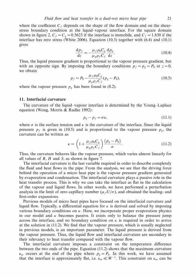
Thus, the curvature behaves like the vapour pressure, which varies almost linearly forall values of R, H and S, as shown in figure 7.

The interfacial curvature is the last variable required in order to describe completelythe fluid and heat flows in the pipe. From the analysis, we see that the driving forcebehind the operation of a micro heat pipe is the vapour pressure gradient generatedby evaporation and condensation. The interfacial curvature plays a passive role in theheat transfer process. This is why we can take the interface as flat in the calculationof the vapour and liquid flows. In other words, we have performed a perturbationanalysis in the limit of zero capillary number (µf U/σ ), and obtained the leading- andfirst-order expansions.

Previous models of micro heat pipes have focused on the interfacial curvature andliquid flow. Typically, a differential equation for κ is derived and solved by imposingvarious boundary conditions on κ . Here, we incorporate proper evaporation physicsin our model and κ becomes passive. It exists only to balance the pressure jumpacross the interface, and no boundary condition on κ is required in order to arriveat the solution in (11.2). We find that the vapour pressure, which is usually neglectedin previous models, is an important parameter. The liquid pressure is derived fromthe vapour pressure. Thus, the liquid flow and interfacial curvature are secondary intheir relevancy to heat transfer compared with the vapour flow.

The interfacial curvature imposes a constraint on the temperature differencebetween the two ends of the pipe. Equation (11.2) shows that the maximum curvatureκm occurs at the end of the pipe where pg = Ph. In this work, we have assumedthat the interface is approximately flat, i.e. κm � W −1. This constraint on κm can be


converted into a limit on (Th − T0) using (8.1):

Th − T0

T0

� σ

ρ0hfgW

(H

Nu − 1

)(1 +

µf ρ0Cg

µgρf Cf

)−1

. (11.3)

This condition makes explicit how small (Th − T0) need be for our analysis to hold.

12. DiscussionThe first part of this work studies fluid motion and heat transfer in a cross-sectional

plane of the dual-wet micro heat pipe. Velocity, pressure and temperature gradientsin the axial direction are assumed negligible compared with the in-plane gradients.This is valid if the length of the pipe is much longer than its width. Thus, the resultsobtained in § 2 to 5 are the leading-order solutions in the limit L/W → ∞.

When we analyse liquid flow and heat transfer in the cross-sectional plane, thetwo-dimensional domain is taken to be unbounded vertically (figure 3). Liquid isassumed to enter at the bottom and leave at the top as vapour. This assumptionof unbounded domain does not affect the results significantly. As shown in § 4,the interfacial temperature has an inner and outer structure. The inner region isnot affected by the domain shape. The outer solution does depend on the domainshape, and the unbounded domain allows an analytical solution of the temperaturefield. However, since the dominant contribution to evaporation comes from the innerregion, and this dominant evaporation term can be the only term used in § 6 to 11,the unbounded-domain assumption does not affect the final solution. It also has noeffect on the liquid motion induced by evaporation and the Marangoni stress, becausethese flows to leading order in E−1 occur only in the inner region (see the Appendix).Hence, the simplification gained from the assumption of unbounded domain justifiesits usage.

Convective heat transfer is negligible in the two-dimensional problem because thePeclet number Pe � 1. The Peclet number (Pe = UMW/αT E, where αT is the liquidthermal diffusivity) measures the ratio of convective to conductive heat transfer. ThisPeclet number is defined using the Marangoni velocity UM (which is an order largerthan the evaporative velocity scale U ) and the length scale E−1W in the inner region(because the Marangoni flow is non-zero only in the inner region). We can estimatethe Evaporation number E and the Marangoni number M for our dual-wet microheat pipe using experimentally measured values in table 1: E = 1820 and M =38.9.The velocity scale U in (3.1) is proportional to pe − pg , which peaks at the pipe end.Thus, the maximum velocity scale is

Um =c

ρf

(pe − Ph) =cρ0hfg (H − Nu + 1)

ρf H

(Th − T0

T0

), (12.1)

where pe in (6.2) and (Ph − P0) in (8.1) have been substituted. For our analysis to bevalid, the temperature difference Th − T0 must obey (11.3). This means

Um � cσ (H − Nu +1)

ρf W (Nu − 1)

(1 +

µf ρ0Cg

µgρf Cf

)−1

, (12.2)

which translates into Pe � 1.02, where we have taken αT =1.07 × 10−7 m2 s−1 formethanol, Cf =Cg , and H = 0. Other parameter values are given in table 1. Thus,convective heat transfer is indeed negligible in the two-dimensional problem.


Experiment Experiment Experiment ExperimentParameters P1 P2 LB1 LB2 Dual-wet

W (×10−6 m) 22.5 30.0 61.0 126 50L (×10−3 m) 10.0 10.0 10.0 10.0 25Af (×10−9 m2) 0.198 0.631 2.50 16.4 10Aw (×10−6 m2) 0.190 0.252 0.235 0.512 0.2T0 (K) 315.0 310.0 325.0 317.0 300µg (×10−5 kg m−1 s−1) 1.00 1.00 1.08 1.00 1.00µf (×10−5 kg m−1 s−1) 58.4 58.4 67.7 42.6 58.4σ (×10−3N m−1) 22.6 22.6 17.7 22.6 22.6dσ

dT(×10−3 N m−1 K−1) −0.190 −0.190 −0.080 −0.190 −0.190

ρe or ρ0 (kgm−3) 1.29 1.29 1.44 1.29 1.29ρf (kgm−3) 791 791 760 791 791hfg (×103 J kg−1) 1100 1100 846 1100 1100kw (Wm−1 K−1) 148 148 148 148 148kf (Wm−1 K−1) 0.200 0.200 0.177 0.194 0.200c(s m−1) 0.00140 0.00140 0.00165 0.00140 0.0014Cg 1.54 0.671 0.692 0.661 0.5623α 1.00 1.00 1.00 1.00 1.00E 780 1060 1800 4480 1820M 40.8 40.2 14.5 56.3 38.9S 0.00225 0.00300 0.00610 0.0126 0.002R 0.673 0.503 0.0418 0.00196 0.506H 8.97 9.47 116 1400 79.7

W is defined as the radius of the largest inscribed sphere for the triangular and rectangular pipes.Af for the four experiments is calculated assuming two-dimensional equilibrium circular meniscus(equation (A1) in Wong et al. 1995).Cg is found assuming that the unidirectional vapour flow occupies the complete cross-sectional area.E and M are calculated using (3.9) with Tp replaced by T0.

Table 1. Two experiments from Peterson et al (1993) (P1 and P2), two from Le Berre et al.(2003) (LB1 and LB2), and a dual-wet micro heat pipe.

The inertia effect is also negligible in the two-dimensional problem because theReynolds number (Re = ρf UMW/µf E) is small. The Marangoni velocity MU and theinner length scale E−1W are again used. The constraint on the maximum velocity scalein (12.2) gives Re � 0.15, assuming again Cf = Cg and H = 0, and using the parametervalues from table 1. Thus, the inertia effect is negligible in the two-dimensionalproblem. Furthermore, the Marangoni flow is decoupled from the evaporation-inducedflow, and thus any inertia effect on the Marangoni flow will have no effect on theevaporation rate.

Gravity is also not important in the two-dimensional problem because the interfaceis almost flat and because the temperature variation is small so that buoyancy can beneglected.

The total evaporation rate in a cross-sectional plane of the dual-wet micro heatpipe is of order E−1 lnE, which comes from the inner region near the contact line.The normalized temperature varies smoothly in the inner region from 1 at the wallto 0 away from the wall. This is a result of the kinetic equation of evaporation.Without the kinetic equation, a non-integrable singularity in temperature appears atthe contact line; the temperature jumps at the contact line from 1 at the wall to0 at the interface. The wall is assumed isothermal, but this is not the reason for


the inner region to exist. Even if the isothermal condition is imposed at a distanceaway from the solid–liquid interface, the inner region still persists (Morris 2000). Theinner region also exists if the contact angle is decreased from 90◦ to 0 (Morris 2000;Ajaev & Homsy 2006). Thus, the inner region is intrinsic to evaporation near a solidwall.

The equilibrium vapour pressure at the hot end of a micro heat pipe is higherthan that at the cold end, and this pressure difference is the basic driving forcebehind the operation of the pipe. Because the vapour can flow from the hot end tothe cold end, the vapour pressure at the hot end cannot maintain the equilibriumvalue; this drop in vapour pressure below the equilibrium value induces continuousevaporation at the hot end. From the two-dimensional analysis at a cross-sectionalplane, we find that the interfacial evaporation comes mainly from a small region nearthe contact line. We assume that a similar process occurs near the cold end, i.e. thevapour condenses in the inner region of the interface. As a result, the temperature andpressure distributions along the pipe are skew-symmetric about the mid-point of thepipe. There are other modes of condensation on a wall, such as drop-wise or film-wisecondensation (Carey 1992). However, since the upper pipe wall is non-wetting, it isdifficult to form a continuous film. Even if a droplet is formed on the wall, it willhave high surface curvature given the large contact angle, and the drop pressure willbe much higher than the vapour pressure. This will make continuous deposition onthe droplet unfavourable (Carey 1992). Thus, the drop-wise condensation will havenegligible contribution. Therefore, the problem discussed here is skew-symmetric, andonly half of the micro heat pipe is considered.

An effective thermal conductivity can be defined for the dual-wet pipe as

ke =qL

AT (Th − T0)=

(Awkw + Af kf

AT

)q

qc

, (12.3)

where AT is the total cross-sectional area including the liquid, vapour, and wall. Theheat rate ratio q/qc (= Nu) depends on three dimensionless numbers: the heat-pipenumber H , the interfacial evaporation resistance ratio R, and the aspect ratio ofthe pipe S, as given in (7.4). Figure 5 shows that Nu � 1 for HR � 1. Thus, ke canbe much larger than either kw or kf if the pipe is constructed and operated withthe proper values of H , R, and S. Furthermore, these dimensionless numbers areindependent of the temperature difference (Th − T0) between the two ends of the pipe.Thus, driving the pipe at larger temperature differences will not improve the effectivethermal conductivity. An effective heat transfer coefficient he can also be defined as

he =q

AT (Th − T0)=

ke

L. (12.4)

A thermal boundary layer appears near the pipe end as the heat-pipe numberH → ∞. The width of the layer scales as (HR)−1/2L, which becomes vanishinglysmall as H → ∞. However, § 2 to 5 we have assumed that the axial gradients arenegligible compared with the cross-stream gradients, and § 6 to 11 we have taken thetemperature variation along the pipe to be one-dimensional. This is correct if the axialvariation of Tp occurs in a length scale that is large compared with the pipe width W .Thus, for our analysis to be valid, (HR)−1/2L � W . This sets an upper bound on H .

The thermal boundary layer is an indicator of effective heat transfer in micro heatpipes. This is because the boundary layer only appears when vapour flow becomesthe dominant mode of heat transfer. When vapour flow dominates, most of theevaporation occurs near the pipe end, so that the temperature drops rapidly within


a thin boundary layer (figure 6). The case of R =104 in figure 6(c) yields a lineartemperature profile along the pipe even though vapour flow dominates. As explainedin § 7, this unusual behaviour is caused by evaporation at the endwall. At such a largeR value, there is negligible resistance for liquid to evaporate, and thus almost all theevaporation occurs at the endwall, despite the small contact-line length. The largeheat flux carried by the vapour flow demands a large temperature drop just outsidethe pipe end. Thus, the linear temperature profile for R = 104 is caused by the pipehaving an endwall with zero thickness. If the endwall has finite thickness, we expectto see a thermal boundary layer for R � 1 and H � 1. Hence, as a general rule, theexistence of a thermal boundary layer is an indicator of effective heat transfer inmicro heat pipes.

Two micro-heat-pipe arrays were constructed in silicon by Peterson et al. (1993) andtested using methanol as the working fluid. One is made of 39 rectangular channelseach 45 µm wide, 80 µm deep, and 19.7 mm long in a silicon wafer 0.378 mm thick(experiment P1). The other is made of 39 triangular channels each 120 µm wide, 80 µmdeep and 20 mm long in a silicon wafer 0.5 mm thick (experiment P2). The wafer washeated at one end to different temperatures depending on the input power. At theother end, the wafer was cooled to 15 ◦C. Le Berre et al. (2003) built two types ofmicro-heat-pipe arrays in silicon wafers using ethanol or methanol as the workingfluid. One of the arrays has 55 triangular channels each 230 µm wide, 170 µm deepand 20 mm long and with a spacing of 130 µm between two neighbouring channels.The void fraction in the transverse cross-section of the whole array is 8% (experimentLB1). The other array has 25 triangular channels; each is 500 µm wide, 340 µm deepand 20 mm long, and is attached to a smaller side channel (also triangular). Themain triangular channels were filled with vapour and the side channels with liquid.We take the size of the side channel to be a quarter of that of the triangular mainchannel. The void fraction in the transverse cross-section of the whole array is 15%(experiment LB2). Table 1 gives the geometric and physical parameters for the fourexperiments. From the parameters, we can calculate E, M , S, R and H . We findthat for all the experiments, E � 1 and M � 1. This justifies the expansions in thetwo-dimensional analysis. For experiment P1 and P2, R ≈ 0.5 and H ≈ 9. This isconsistent with the observed linear temperature profile along the channels becauseHR ∼ 1. For experiment LB1, H = 116 and R = 0.0418, and for experiment LB2,H = 1400 and R = 0.00196. The observed temperature profile is linear in LB1 andshows a small drop near the hot end in LB2. Although the product HR ∼ 1 in bothLB1 and LB2, the large H value in LB2 suggests probable heat transfer by vapourflow, and therefore the emergence of a thermal boundary layer.

13. ConclusionsA dual-wet micro heat pipe is proposed with simplified interfacial geometry while

retaining the essential physics. Sections 2 to 5 study fluid motion and heat conductionin a cross-section plane in the heated half of the pipe. The wall temperature Tp isassumed known and the vapour pressure pg is decreased below the equilibrium vapourpressure pe to induce evaporation. Two dimensionless parameters emerge: E and M ,and the problem is solved in the limits E → ∞ and M → ∞. The temperature field hasan inner region near the contact line defined by the length scale E−1W . This innerregion is intrinsic to evaporation near a contact line and is independent of the outerdomain shape. In the inner region, the dimensionless interfacial temperature variessmoothly from 1 at the wall to 0 away from the wall. This creates a Marangoni flow


and an evaporation-induced flow, which are solved at different levels of expansion inM . It is found that the total evaporation rate Q∗ ∼ E−1 lnE to leading order. This isthe evaporation rate per unit contact-line length.

Sections 6 to 11 determine the temperature distribution and vapour and liquidflows along the pipe. Thermal energy is transferred along the pipe by vapour flow(latent heat) and by conduction in the liquid and wall. These two modes of heattransfer always add up to a constant (q) at every point along the pipe because thepipe is insulated at the outer wall. The two transfer modes are coupled by the localevaporation rate Q found in § 2 to 5. The evaporation rate Q depends on the localvapour pressure pg and pipe (liquid and wall) temperature Tp . This is an importantfinding of our analysis because it leads to a thermal boundary layer near the pipeend.

Analytical solutions are found for all dependent variables: Tp (pipe temperature),pg (vapour pressure), Vg (vapour flow rate), pf (liquid pressure), Vf (liquid flowrate), and κ (interfacial curvature). The solutions depend on three dimensionlessparameters: H , R, and S. If HR � 1, a thermal boundary layer appears near thepipe end in which the pipe temperature Tp varies rapidly (figure 6). The widthof the layer scales as (HR)−1/2L. A similar boundary layer exists at the cold end.Outside the boundary layers, Tp varies linearly with a gradual slope. Thus, theseregions correspond to the evaporative, adiabatic and condensing regions commonlyobserved in heat pipes. This is the first time that the distinct regions are capturedby a single temperature distribution, without prior assumptions of their existence. IfHR ∼ 1 or less, then Tp decreases almost linearly from the hot end to the cold. Weanalyse four micro-heat-pipe arrays studied experimentally and find HR ∼ 1 (table1). This explains the absence of the adiabatic region in most of those micro heatpipes.

The vapour pressure pg varies almost linearly along the pipe and is insensitive tothe value of H (figure 7), whereas a boundary layer exists for the vapour flow rateVg for H � 1 (figure 8). The liquid volume flow rate Vf is proportional to Vg atevery point along the pipe because the pipe is a closed system. The liquid pressurepf is found from Vf and is therefore proportional to pg . The difference pg − pf givesthe interfacial curvature κ , which varies almost linearly along the pipe and is alsoinsensitive to H . Our analysis shows that the operation of a micro heat pipe is drivenby the vapour pressure difference between the hot and cold ends. The interfacialcurvature plays a passive role in the heat transfer process, contrary to conventionalbeliefs.

The heat rate q is constant along the pipe because the pipe is assumed to beinsulated at the outer wall. An analytic solution is found for Nu = q/qc, where qc isthe conductive heat rate through the pipe. We find that as H → ∞, Nu ∼ H , and asH → 0, Nu → 1 (figure 5). Thus, micro heat pipes should be designed and operatedwith HR � 1 to benefit from the evaporative heat transfer.

This work was supported by NASA (NAG3-2361 to H. W.), Louisiana SpaceConsortium (LaSPACE) Research Enhancement Awards (to H. W.), and a LouisianaEconomic Development Award (to J. Z.).

Appendix A. Velocity field in the cross-sectional planeThe velocity field in the cross-sectional plane is expanded in the limit M → ∞ as

u∗ = u0M + u1 + · · · (A 1)


The velocity expansions u0 and u1 are zero in the outer region x∗ � E−1 and y∗ � E−1

defined in § 4. These velocity expansions in the limit M → ∞ are also the zero-orderterm in the expansion in the limit E → ∞. However, to zero order in E−1, the liquidvelocity is zero in the outer region; the velocity components are zero at the wall asstated in (3.6), at the symmetry plane as stated in (3.7), and at the interface as statedin (3.8) (because t0 = 0 and ∂t0/∂x∗ = 0 at the interface). Also, in (3.10a), the totalevaporation rate Q∗ ∼ E−1 in the outer region as shown in § 5, which means thatQ∗ = 0 to zero order in E−1. Hence, u0 and u1 are zero in the outer region, and onlytheir solutions in the inner region are studied below.

A.1. Zero-order velocity u0 in the inner region

In component form, u0 = u0 i + v0 j . At the liquid–vapour interface Y = 0, (3.8) gives

v0 = 0,∂u0

∂Y=

∂τ

∂X. (A 2)

Thus, there is zero evaporation at this order, and the flow is driven by the Marangonistress.

A stream function is defined in terms of the inner variables:

u0 =∂ψ0

∂Y, v0 = − ∂ψ0

∂X. (A 3)

The streamfunction obeys

∇4ψ0 = 0. (A 4)

No slip at the wall X = 0 requires

ψ0 = 0,∂ψ0

∂X= 0. (A 5)

At the liquid–vapour interface Y = 0, (A2) becomes

ψ0 = 0,∂2ψ0

∂Y 2=

∂τ

∂X. (A 6)

The velocity components decay to zero far from the corner. Thus, as X → ∞ orY → ∞,

∂ψ0

∂Y→ 0,

∂ψ0

∂X→ 0. (A 7)

The Marangoni stress at the interface is the only non-zero term and it drives the flow.The unbounded domain is treated in two ways. First, coordinates X and Y are

exponentially contracted by defining

ξ = ln (X + 1) , η = ln (Y +1) . (A 8)

Secondly, a far-field asymptotic solution is found and used as boundary conditionsat large but finite (ξ , η). The shear stress at the interface is non-zero near the corner,and decays to zero far from the corner, as shown by (A6). Thus, far from the corner,the shear stress can be viewed as a point force. The streamfunction generated by apoint force pointing towards a solid wall is (Liron & Blake 1981)

ψ0 = f Y

{2DX

Y 2 + (X + D)2− 1

2ln

[Y 2 + (X + D)2

Y 2 + (X − D)2

]}. (A 9)

where f is the strength of the point force and D is the distance between the pointforce and the wall. The strength f is found from the shear stress boundary condition


0 2

2

4

Y

6

8

10

4 6X

8 10

–0.085

–0.08

–0.07

–0.06

–0.05

–0.04

–0.03

–0.02

–0.01

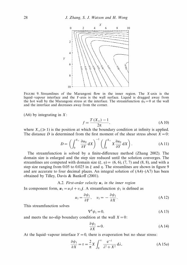
Figure 9. Streamlines of the Marangoni flow in the inner region. The X-axis is theliquid–vapour interface and the Y -axis is the wall surface. Liquid is dragged away fromthe hot wall by the Marangoni stress at the interface. The streamfunction ψ0 = 0 at the walland the interface and decreases away from the corner.

(A6) by integrating in X:

f =T (X∞) − 1

2π, (A 10)

where X∞(� 1) is the position at which the boundary condition at infinity is applied.The distance D is determined from the first moment of the shear stress about X = 0:

D =

(∫ X∞

0

∂u0

∂YdX

)−1 (∫ X∞

0

X∂u0

∂YdX

). (A 11)

The streamfunction is solved by a finite-difference method (Zhang 2002). Thedomain size is enlarged and the step size reduced until the solution converges. Thestreamlines are computed with domain size (ξ , η) = (6, 6), (7, 7) and (8, 8), and with astep size ranging from 0.05 to 0.025 in ξ and η. The streamlines are shown in figure 9and are accurate to four decimal places. An integral solution of (A4)–(A7) has beenobtained by Tilley, Davis & Bankoff (2001).

A.2. First-order velocity u1 in the inner region

In component form, u1 = u1 i + v1 j . A streamfunction ψ1 is defined as

u1 =∂ψ1

∂Y, v1 = − ∂ψ1

∂X. (A 12)

This streamfunction solves

∇4ψ1 = 0, (A 13)

and meets the no-slip boundary condition at the wall X = 0:

∂ψ1

∂X= 0. (A 14)

At the liquid–vapour interface Y =0, there is evaporation but no shear stress:

∂ψ1

∂X= τ =

2

πX

∫ ∞

0

e−λ

λ2 + X2dλ, (A 15a)


0 2

2

4

Y

X

6

8

10

4 6 8 10–1.7

–1.6–1.5–1.4–1.3–1.2–1.1–0.9–0.8–0.7–0.6–0.5–0.4–0.3–0.2–0.1

–0.05

–0.02

–1

Figure 10. Streamlines of the evaporation-induced flow in the inner region near the contactline. The X-axis is the liquid–vapour interface and the Y -axis is the wall surface. Thestream-function ψ1 = 0 at the wall and decreases away from the wall.

∂2ψ1

∂Y 2= 0. (A 15b)

Far from the corner, as X or Y → ∞,

∂ψ1

∂Y→ 0,

∂ψ1

∂X→ 0. (A 16)

Thus, liquid flow at the first order is driven by evaporation at the interface.The unbounded domain is treated by the same two methods: coordinate contraction

as in (A8), and a far-field asymptotic solution. Evaporation at the interface occursmainly near the wall, and decays to zero far from the wall. Thus, the liquid velocitiesfar from the corner are the same as those of a sink flow. The radial velocity generatedby a line sink on a planar wall is (White 2006)

ur = − 4F

πrsin2 θ, (A 17)

where F is the sink strength or the volume flow rate per unit length, r is the radialdistance, and θ starts from the wall. This sink flow applies because the interface actslike a symmetry plane. The sink strength is found by equating the leakage rates:

F =

∫ X∞

0

Ti(X, 0) dX, (A 18)

where X∞ is the position of the outer domain boundary. Thus, at the outer domainboundaries,

∂ψ1

∂Y= ur cos θ,

∂ψ1

∂X= − ur sin θ. (A 19)

The streamfunction is solved by a finite-difference method (Zhang 2002). The accuracyis verified by enlarging the domain and reducing the step size. The streamlines arecomputed with domain size (ξ , η) = (5, 5), (6, 6), (7, 7) and (8, 8), and with step sizeof 0.1, 0.05 or 0.0125 in ξ and η. The results are accurate to four decimal places. Aplot of the streamlines is shown in figure 10.


REFERENCES

Ajaev, V. S. & Homsy, G. M. 2006 Modeling shapes and dynamics of confined bubbles. Annu. Rev.Fluid Mech. 38, 277–307.

Badran, B., Gerner, F. M., Ramadas, P., Henderson, T. & Baker, K. W. 1997 Experimental resultsfor low-temperature silicon micromachined micro heat pipe arrays using water and methanolas working fluids. Experimental Heat Transfer 10, 253–272.

Barrett, J. & Clement, C. 1992 Kinetic evaporation and condensation rates and their coefficients.J. Colloid Interface. Sci. 150, 352–364.

Burelbach, J. P., Bankoff, S. G. & Davis, S. H. 1988 Nonlinear stability of evaporating/condensingliquid films. J. Fluid Mech. 195, 463–494.

Carey, V. P. 1992 Liquid–vapor Phase-change Phenomena: An Introduction to the Thermophysics ofVaporization and Condensation Processes in Heat Transfer Equipment. Taylor & Francis.

Churchill, R. V. & Brown, J. W. 1984 Complex Varibales and Applications. McGraw–Hill.

Cotter, T. R. 1984 Principles and properties of micro heat pipes. Proc. Intl Heat Pipe Conf.Tsukuba, Japan.

Darhuber, A., Troian, S. M. & Reisner, W. W. 2001 Dynamics of capillary spreading alonghydrophilic microstripes. Phys. Rev. E 64, 031603.

Faghri, A. 1995 Heat Pipe Science and Technology. Taylor & Francis.

Gau, H., Herminghaus, S., Lenz, P. & Lipowsky, R. 1999 Liquid morphologies on structuredsurfaces: from microchannels to microchips. Science 283, 46–49.

Groll, M., Schneider, M., Sartre, V., Zaghdoudi, M. C. & Lallemand, M. 1998 Thermal controlof electronic equipment by heat pipes. Rev. Gen. Therm. 37, 323–352.

Ha, J. M. & Peterson, G. P. 1998 The heat transfer capacity of micro heat pipes. Trans. ASME C:J. Heat Transfer 120, 1064–1071.

Khrustalev, D. & Faghri, A. 1994 Thermal analysis of a micro heat pipe. Trans. ASME C:J. Heat Transfer 116, 189–198.

Launay, S., Sartre, V. & Lallemand, M. 2004 Hydrodynamic and thermal study of a water-filledmicro-heat-pipe array. J. Thermophys. Heat Transfer 18, 358–363.

Le Berre, M., Launay, S., Sartre, V. & Lallemand, M. 2003 Fabrication and experimentalinvestigation of silicon micro heat pipes for cooling electronics. J. Micromech. Microengng. 13,436–441.

Levich, V. G. 1962 Physicochemical Hydrodynamics. Prentice–Hall.

Liron, N. & Blake, J. R. 1981 Existence of viscous eddies near boundaries. J. Fluid Mech. 107,109–129.

Longtin, J. P., Badran, B. & Gerner, F. M. 1994 A one-dimensional model of a micro heat pipeduring steady-state operation. J. Heat Transfer 116, 709–715.

Morris, S. J. S. 2000 A phenomenological model for the contact region of an evaporating meniscuson a superheated slab. J. Fluid Mech. 411, 59–89.

Peterson, G. P. 1994 An Introduction to Heat Pipes. John Wiley.

Peterson, G. P., Duncan, A. B. & Weichold, M. H. 1993 Experimental investigation of micro heatpipes fabricated in silicon wafers. J. Heat Transfer 115, 751–756.

Plesset, M. S. & Prosperetti, A. 1976 Flow of vapour in a liquid enclosure. J. Fluid Mech. 78,433–444.

Sobhan, C. B., Rag, R. L. & Peterson, G. P. 2007 A review and comparative study of theinvestigations on micro heat pipes. Intl J. Energy Res. 31, 664–688.

Suman, B. & Kumar, P. 2005 An analytical model for fluid flow and heat transfer in a micro-heatpipe of polygonal shape. Intl J. Heat Mass Transfer 48, 4498–4509.

Tilley, B. S., Davis, S. H. & Bankoff, S. G. 2001 Unsteady Stokes flow near an oscillating heatedcontact line. J. Fluid Mech. 438, 339–362.

Wayner, P. C. 1993 Spreading of a liquid film with a finite contact angle by the evaporation/condensation process. Langmuir 9, 294–299.

White, F. M. 2006 Viscous Fluid Flow. McGraw–Hill.

Wong, H., Morris, S. & Radke, C. J. 1992 Three-dimensional menisci in polygonal capillaries.J. Colloid Interface Sci. 148, 317–336.


Wong, H., Radke, C. J. & Morris, S. 1995 The motion of long bubbles in polygonal capillaries.1. Thin films. J. Fluid Mech. 292, 71–94.

Wu, D. & Peterson, G. P. 1991 Investigation of the transient characteristics of a micro heat pipe.J. Thermophys Heat Transfer 5, 129–134.

Wu, Q. & Wong, H. 2004 A slope-dependent disjoining pressure for non-zero contact angles.J. Fluid Mech. 506, 157–185.

Zhang, J. 2002 A model of heat and mass transfer in an idealized micro heat pipe. Master, Thesis,Louisiana State University.

fluid flow and heat transfer in a dual-wet micro heat pipe

Documents