fluid characterisation and drop impact in inkjet printing for organic
TRANSCRIPT

Fluid characterisation and drop impact in inkjet printing for organic semiconductor devices
Sungjune Jung St John’s College
This dissertation is submitted for the degree of Doctor of Philosophy
Manufacturing and Management Division
Department of Engineering University of Cambridge
April 2011

i
Declarations
This dissertation is the result of my own work and includes nothing which is the outcome of
work done in collaboration except where specifically indicated in the text. The length of this
dissertation is 42,721 words with 104 figures and 4 tables. It is not substantially the same as
any I have submitted for a degree or diploma or any other qualification at any other university.

ii
Acknowledgements
I would like to thank Korea Institute for Advancement of Technology, Cambridge Display
Technology, Ltd and Cambridge Overseas Trust for the financial support which made
possible the research and completion of this dissertation.
I am most indebted to my supervisor, Professor Ian Hutchings. He has been a pillar of
stability through all my ups and downs, and I am truly grateful for his generosity with his
time, insightful comments, unfailing enthusiasm, and friendship. I am grateful for the
assistance from my colleagues at Inkjet Research Centre: Dr Graham Martin, Dr Steve Hoath,
Dr Wen-Kai Hsiao, Dr Rafael Castrejon-Pita, Dr Eleanor Betton and Miss Jenny Hornett.
They all were with me from the very beginning to the end and provided the much-needed
encouragement and thoughtful advice for me to continue my research. Specially, Dr Martin
co-supervised me with his industrial experience, and Dr Hoath helped me a lot with his
insight into polymer science and gave me invaluable comments on my works and writings. I
offer my deepest appreciation to all of them.
I also thank Professor Malcolm Mackley, Dr Tri Tuladhar (now at Xaar plc), Dr Damien
Vadillo and Amit Mulji for their insight into ink rheology and helps with rheological
measurements.
And last but not least, I would like express my heartfelt gratitude to all my family and friends
for their encouragement and support. Specially, I am deeply thankful of my wife Mira for her
full support, wisdom and prayers, and of my new-born baby Jisu. I love you both so much.

iii
List of symbols (Roman)
A Area c Polymer concentration c* Critical concentration Ca Capillary number D Drop diameter Do Drop diameter at impact Dj Jet diameter Dmid Mid-filament diameter Dp Piston diameter De Deborah number EK, EG, ES, ED Kinetic, gravitational, surface tension and viscous dissipation energy El Elasticity number Ec Elasto-capillary number G Spring constant f Frequency G′ Viscous modulus G″ Elastic modulus g Acceleration due to gravity h Drop height k Coefficient in Tanner’s law kB Boltzmann constant Lj Jet length L0 Characteristic length MW Molecular weight NA Avogadro’s number Oh Oh number n Power-law index T Absolute temperature (K) t Time tv Viscous timescale te Elastic timescale tc Capillary timescale V Drop speed Vo Drop speed at impact Vj Jet speed VT Jet shortening speed given by Taylor model Re Reynolds number We Weber number Wi Weissenberg number Z Z number (1/Oh)

iv
List of symbols (Greek)
α Half-angle between two impinging jets β Spreading factor (= D/Do) β* Maximum spreading factor at the end of spreading phase β∞ Equilibrium spreading factor � Shear strain �� Shear rate η Viscosity η0 Low-shear viscosity ηΕ Extensional viscosity ηs Solvent viscosity η* Complex viscosity [η] Intrinsic viscosity λ Relaxation time λz Zimm relaxation time λm Most unstable wavelength on a cylindrical column of liquid ν Solvent quality exponent ρ Density σ Surface tension τ Dimensionless time τ∗ Dimensionless time at β* τ∞ Dimensionless time at β∞ τs Shear stress θa Advancing contact angle θd Dynamic contact angle θeq Equilibrium contact angle θmax Maximum fishbone angle θr Receding contact angle ω Angular frequency Ψ Sum of three energies contributed by three interfaces

v
Contents 1. Introduction ................................................................................................................. 1
1.1 Research background .................................................................................................. 1
1.2 Research questions ...................................................................................................... 3
1.3 Outline of the thesis .................................................................................................... 3
2. Background to inkjet printing technology ................................................................... 5
2.1 Introduction ................................................................................................................. 5
2.2 Working principles of inkjet print heads ..................................................................... 5
2.2.1 Continuous inkjet ................................................................................................. 6
2.2.2 Thermal inkjet ...................................................................................................... 8
2.2.3 Piezoelectric inkjet ............................................................................................. 10
2.3 Inkjet printing for organic semiconductor devices .................................................... 14
2.3.1 Polymer organic light-emitting diodes (P-OLEDs) ........................................... 14
2.3.2 Polymer thin-film transistors .............................................................................. 18
2.3.3 Solar cells ........................................................................................................... 23
2.4 Collision of two impinging jets ................................................................................. 24
2.5 The drop impact process in inkjet printing ............................................................... 25
2.5.1 Drop impact process ........................................................................................... 25
2.5.2 Models for the prediction of maximum drop spreading ..................................... 33
2.6 High–speed imaging techniques ............................................................................... 37
2.6.1 Cinematography ................................................................................................. 37
2.6.2 Flash–Photography ............................................................................................. 39
3. Fluid characterisation ................................................................................................ 41
3.1 Introduction ............................................................................................................... 41
3.2 Viscoelasticity ........................................................................................................... 41
3.3 Methods for characterisation of viscoelasticity ......................................................... 45
3.3.1 Drag flow rheometer .......................................................................................... 45

vi
3.3.2 Piezo axial vibrator ............................................................................................ 45
3.3.3 Filament stretching rheometer ............................................................................ 47
3.4 Dimensionless groups relevant to drop generation and impact................................. 49
4. Materials and experimental methods......................................................................... 54
4.1 Introduction ............................................................................................................... 54
4.2 Fluids and substrates ................................................................................................. 54
4.2.1 Fluids .................................................................................................................. 54
4.1.2 Substrates ........................................................................................................... 57
4.3 Rheological measurements ........................................................................................ 57
4.3.1 Apparent viscosity .............................................................................................. 57
4.3.2 Piezo-axial vibrator ............................................................................................ 59
4.3.3 Filament stretching rheometer ............................................................................ 59
4.4 Experimental arrangement for collision of two liquid jets ........................................ 63
4.5 Experimental system and imaging processing technique for drop impact study ...... 67
4.4.1 Drop deposition and high-speed imaging system .............................................. 67
4.4.2 Imaging processing technique ............................................................................ 70
5. Collision of two liquid jets: I. Newtonian fluid ........................................................ 74
5.1 Introduction ............................................................................................................... 74
5.2 Results ....................................................................................................................... 75
5.2.1 Effects of asymmetry in the collision of two identical jets ................................ 75
5.2.2 Effects of jet length ............................................................................................ 78
5.2.3 Effects of viscosity ............................................................................................. 81
5.2.4 Sheet and drop sizes under conditions of maximum fishbone angle ................. 84
5.2.5 Induction of the fishbone instability by external perturbation ........................... 85
5.3 Discussion ................................................................................................................. 86
5.3.1 Maximum fishbone angle and drop size ............................................................ 86
5.3.2 Asymmetrical collision of the jets ...................................................................... 86
vii
5.3.3 Fishbone instability ............................................................................................ 89
5.3.4 What causes the fishbone pattern? ..................................................................... 92
5.4 Conclusions ............................................................................................................... 94
6. Collision of two liquid jets: II. Non-Newtonian fluid ............................................... 96
6.1 Introduction ............................................................................................................... 96
6.2 Results ....................................................................................................................... 97
6.2.1 Qualitative observations ..................................................................................... 97
6.2.2 Influence of viscoelasticity on the fishbone pattern ......................................... 100
6.2.3 Correlation between θmax and high frequency viscoelastic properties ............. 102
6.2.4 Variation of droplet diameter and spacing with fluid elasticity ....................... 105
6.2.5. Jetting behaviour ............................................................................................. 105
6.3 Discussion ............................................................................................................... 108
6.3.1 Effect of elasticity on the occurrence of the fishbone pattern .......................... 108
6.3.2 Variation of θmax with polymer concentration .................................................. 109
6.3.3 Correlation of θmax with jetting performance ................................................... 111
6.4 Conclusions ............................................................................................................. 113
7. Drop impact dynamics: I. Newtonian fluid ............................................................. 114
7.1 Introduction ............................................................................................................. 114
7.2 Results ..................................................................................................................... 115
7.2.1 Jetting behaviour and drop generation ............................................................. 115
7.2.2 Experimental observations of impact ............................................................... 118
7.2.3 Effect of initial speed on drop impact and spreading ....................................... 122
7.2.4 Effect of surface wettability on drop impact and spreading ............................ 124
7.2.5 Effect of fluid properties on drop impact and spreading .................................. 126
7.3 Discussion ............................................................................................................... 127
7.3.1 Impact process .................................................................................................. 127

viii
7.3.2 Prediction of maximum spreading factor ......................................................... 128
7.3.3 Comparison between the impact of mm-sized and smaller drops .................... 130
7.4 Conclusions ............................................................................................................. 132
8. Drop impact dynamics: II. Non-Newtonian fluid ................................................... 134
8.1 Introduction ............................................................................................................. 134
8.2 Results ..................................................................................................................... 134
8.2.1 Jetting behaviour .............................................................................................. 134
8.2.2 Deposition behaviour ....................................................................................... 139
8.3 Discussion ............................................................................................................... 141
8.3.1 Effect of polymer on jetting ............................................................................. 141
8.3.2 Effect of polymer on drop impact .................................................................... 142
8.4 Conclusions ............................................................................................................. 147
9. Summary and overall discussion ............................................................................. 148
Appendix ........................................................................................................................... 155
References ......................................................................................................................... 157
List of Publications ........................................................................................................... 168
ix
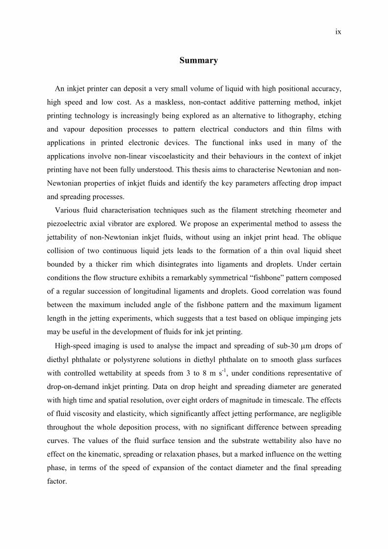
Summary
An inkjet printer can deposit a very small volume of liquid with high positional accuracy,
high speed and low cost. As a maskless, non-contact additive patterning method, inkjet
printing technology is increasingly being explored as an alternative to lithography, etching
and vapour deposition processes to pattern electrical conductors and thin films with
applications in printed electronic devices. The functional inks used in many of the
applications involve non-linear viscoelasticity and their behaviours in the context of inkjet
printing have not been fully understood. This thesis aims to characterise Newtonian and non-
Newtonian properties of inkjet fluids and identify the key parameters affecting drop impact
and spreading processes.
Various fluid characterisation techniques such as the filament stretching rheometer and
piezoelectric axial vibrator are explored. We propose an experimental method to assess the
jettability of non-Newtonian inkjet fluids, without using an inkjet print head. The oblique
collision of two continuous liquid jets leads to the formation of a thin oval liquid sheet
bounded by a thicker rim which disintegrates into ligaments and droplets. Under certain
conditions the flow structure exhibits a remarkably symmetrical “fishbone” pattern composed
of a regular succession of longitudinal ligaments and droplets. Good correlation was found
between the maximum included angle of the fishbone pattern and the maximum ligament
length in the jetting experiments, which suggests that a test based on oblique impinging jets
may be useful in the development of fluids for ink jet printing.
High-speed imaging is used to analyse the impact and spreading of sub-30 µm drops of
diethyl phthalate or polystyrene solutions in diethyl phthalate on to smooth glass surfaces
with controlled wettability at speeds from 3 to 8 m s-1, under conditions representative of
drop-on-demand inkjet printing. Data on drop height and spreading diameter are generated
with high time and spatial resolution, over eight orders of magnitude in timescale. The effects
of fluid viscosity and elasticity, which significantly affect jetting performance, are negligible
throughout the whole deposition process, with no significant difference between spreading
curves. The values of the fluid surface tension and the substrate wettability also have no
effect on the kinematic, spreading or relaxation phases, but a marked influence on the wetting
phase, in terms of the speed of expansion of the contact diameter and the final spreading
factor.

Chapter 1 1
1. Introduction
1.1 Research background
Inkjet printing generally involves the generation, control and deposition of sub-100µm
drops of liquid. An inkjet printer can deposit a very small volume of liquid (down to 1
picolitre or a drop diameter ≈ 12 µm) with high positional accuracy, high speed and low cost.
As a maskless, non-contact additive patterning method, this technology is increasingly being
explored as an alternative to lithography, etching and vapour deposition processes to pattern
electrical conductors and thin films with applications in printed electronic devices such as
organic thin-film transistors (OTFTs), plastic organic light emitting diodes (OLEDs), solar
cells, radio frequency identification (RFID) tags, printed circuit boards, memory devices and
sensors (Forrest 2004; Tekin et al. 2008; Singh et al. 2010). Many of the applications of
inkjet printing require a good understanding of drop deposition on to a highly wettable, non-
porous substrate: this involves both the initial impact and spreading stages as well as the later
stages of the wetting process. A polymer OLED display which contains a number of pixels of
organic electroluminescent elements provides a typical example. A hole-injection layer and a
luminescent layer are formed between a cathode and a transparent indium tin oxide (ITO)
anode coated on to a glass substrate. The two layers are deposited by regions of less wettable
material. In order to optimise the printing process it is necessary to understand the whole
process of liquid drop impact including the dynamic behaviour of a drop over a very short
time scale (microseconds) and the much longer wetting process (which typically extends over
several seconds).
The impact of liquid drops on solid surfaces has been extensively studied since
Worthington’s pioneering works more than 130 years ago (Worthington 1876). He showed
the fascinating patterns formed by a liquid drop during impact, based on direct observation of
the phenomena with the naked eye by using short-duration spark illumination to freeze the
image. For decades a substantial amount of experimental, numerical and theoretical studies
have been conducted to identify the important parameters influencing the impact process and

Chapter 1 2
the final outcome of the drop impact for practical applications such as coating, painting, rapid
spray cooling of hot surfaces and quenching of alloys and steel. However, while most of the
earlier experimental studies on drop impact were undertaken with mm-sized drops, to date
few studies have been done to understand the dynamics of a sub-100 µm inkjet-printed drop
on a solid substrate, particularly a viscoelastic polymer drop. The major challenges in
researching this lie in the vast range of time scales involved in the drop impact process (from
< 1 µs up to > 1 s) and the very small size of a printed drop (typically < 50 µm).
Most applications in printed electronics involve polymer-containing functional inks. Inkjet
fluids are usually characterised by their zero-shear viscosity which may not fully reflect the
resistance to flow through the nozzle or the collapse of the ligament. A great deal of study
remains to be done in developing viscoelastic fluid characterisation methods, which will help
enhance our understanding of the impact dynamics of non-Newtonian liquid drops to
facilitate further advances in this very exciting field.
This thesis aims to characterise both the Newtonian and non-Newtonian fluid properties of
inkjet fluids, and to achieve a fuller understanding of the mechanics of the liquid drop impact
process and of fluid/substrate interactions in the context of industrial inkjet printing. To
pursue the goal, the following three pieces of works have been performed.
1. Studies on rheology and rheological measurements relevant to inkjet printing.
Recent literature shows that many functional inks including electroluminescence inks and
conductive inks used in making organic semiconductor devices exhibits viscoelastic
behaviour at high frequency. It is therefore necessary to study the rheology of viscoelastic ink
fluids and to explore various methods to characterise the rheological properties of the fluids
in the context of inkjet printing.
2. The development of a state-of-the-art high-speed optical imaging system.
No experimental apparatus in the past has been used to image the whole impact process of
an inkjet-printed drop on highly wettable surface. Some research groups have focused on
initial impact processes and others on later wetting process. Therefore, it is crucial in drop
impact study to develop a state-of-the-art optical imaging system which enables us to
overcome the challenges of the short length and long time scale.

Chapter 1 3
3. Investigation on drop impact dynamics with various combinations of fluids and
substrates.
Drop impact experiments, which are carried out systematically with appropriate model
fluids with different fluid properties and substrates with different wetting properties, will lead
to successful identification of the key parameters affecting the dynamics of the process.
1.2 Research questions
In order to enhance our understanding of the inkjet drop impact process and to identify all
the relevant factors which influence it, the following research questions will be addressed.
Research question 1: Which techniques can be used to assess the rheological proper-
ties of various functional polymer inks in the context of inkjet printing?
Research question 2: Is there any new simple method to assess the printability of non-
Newtonian inkjet fluids, without using an inkjet print head?
Research question 3: What is the best optical system to acquire high quality images of
sub-50 µm drops over a wide range of time scale (from 100 ns to 10 s) and which image
processing technique can be applied to extract relevant information from the obtained images?
Research question 4: What are the key parameters of Newtonian ink affecting its drop
spreading and wetting behaviour?
Research question 5: How can those parameters contribute to theoretical models for
the whole process of drop impact?
Research question 6: How does the drop impact process vary with impact conditions
for different surfaces?
Research question 7: How do the rheological properties of a viscoelastic ink affect the
impact process?
1.3 Outline of the thesis
This thesis is organised as follows:
Chapters 2 and 3 provide the background and literature review of inkjet printing
technology, fluid characterisation methods relevant to this work, and drop impact and

Chapter 1 4
spreading process. Chapter 2 gives an overview of inkjet printing technology and its recent
applications to printed electronic devices. Literature review on collision of two liquid jets
which will be used later to assess the printability of polymer inks is provided. The drop
impact process and high-speed imaging techniques are also briefly reviewed. Chapter 3
introduces various characterisation methods for viscoelastic inkjet fluids. Dimensionless
numbers for describing flows of Newtonian and non-Newtonian fluids are also introduced.
Chapter 4 presents fluid characterisation methods and a high-speed imaging system used
in this works. Fundamental properties and conditions of the model fluids and substrates used
in the experiments are also presented. Research questions 1 and 3 are addressed in this
chapter.
Chapters 5 and 6 introduce a new experimental method to assess the jetting performance
of fluids for use in drop-on-demand inkjet print heads. The periodic atomisation pattern
produced by the oblique collision of two liquid jets, a so-called ‘fluid fishbone’ pattern, is
effectively exploited for this purpose. Chapter 5 discusses how changes in the various
parameters influence the form of the atomisation pattern and the origin and mechanism of the
periodic atomization. Chapter 6 presents the formation and atomisation of the fluid sheet
created by colliding jets of viscoelastic fluids. This study shows that there is good correlation
between the pattern and the jetting performance of a given fluid from a commercial print
head. Research questions 1 and 2 are addressed in these chapters.
Chapter 7 and chapter 8 aim to answer research question 4 to 7. The spreading and wetting
behaviours of an inkjet-printed drop are investigated. The deposition dynamics of Newtonian
fluids is investigated in Chapter 7. The results are also compared with several theoretical
models and also with experimental results for mm-sized drops. Chapter 8 probes how the
viscoelasticity of non-Newtonian fluids affects the jetting and deposition process.
Chapter 9 summarises the main findings of this thesis and presents the answers to all the
research questions.
Chapter 2 5
2. Background to inkjet printing technology
2.1 Introduction
This chapter explore the literature which is relevant to understanding inkjet printing
technology, processes and applications. It begins with the introduction of two major working
principles of inkjet printing: continuous inkjet printing and drop-on-demand inkjet printing
(thermal and piezo). The recent applications of inkjet printing to the organic semiconductor
devices such as organic light emitting diodes, thin film transistors and solar cells are then
presented in section 2.3. Section 2.4 reviews literature on liquid atomisation produced by
collision of two impinging jets. Finally, in sections 2.5 and 2.6 the dynamics of a fluid drop
impacting on to solid non-porous surfaces and the high-speed imaging technique for studying
the drop impact process are reviewed with relevant literature.
2.2 Working principles of inkjet print heads
The theoretical basis of modern inkjet technology was founded by Lord Rayleigh in a
series of papers on liquid jets and their instability (Rayleigh 1878; Rayleigh 1879; Rayleigh
1882). Although the first inkjet-like recording device using electrostatic forces was invented
by Lord Kelvin in 1858, the first practical inkjet device based on Rayleigh’s principle was
devised in 1951 by Elmqvist of Siemens-Elema (US Patent 2,566,433). A more elaborate
continuous inkjet printer emerged in the early 1960s when Sweet of Stanford University
demonstrated that a series of drops with uniform size and spacing could be generated from a
stream of liquid by applying a regular pressure wave to orifice (Sweet 1965).
Various types of drop-on-demand (DoD) inkjet technologies began to appear from the
1970s. The first piezo-based inkjet printer was designed by Zoltan of the Clevite company in
1972 (US Patent 3, 683, 212). He proposed a squeeze mode of piezo print head, which led to
the later introduction of other types of print heads such as bend mode, push mode and shear
mode. On the other hand, Canon invented the thermal-type inkjet technology, named ‘Bubble
Chapter 2 6
jet’, which generates drops by using the growth and collapse of a vapour bubble in an ink
chamber. Hewlett-Packard also developed similar technology, called ‘Think jet’.
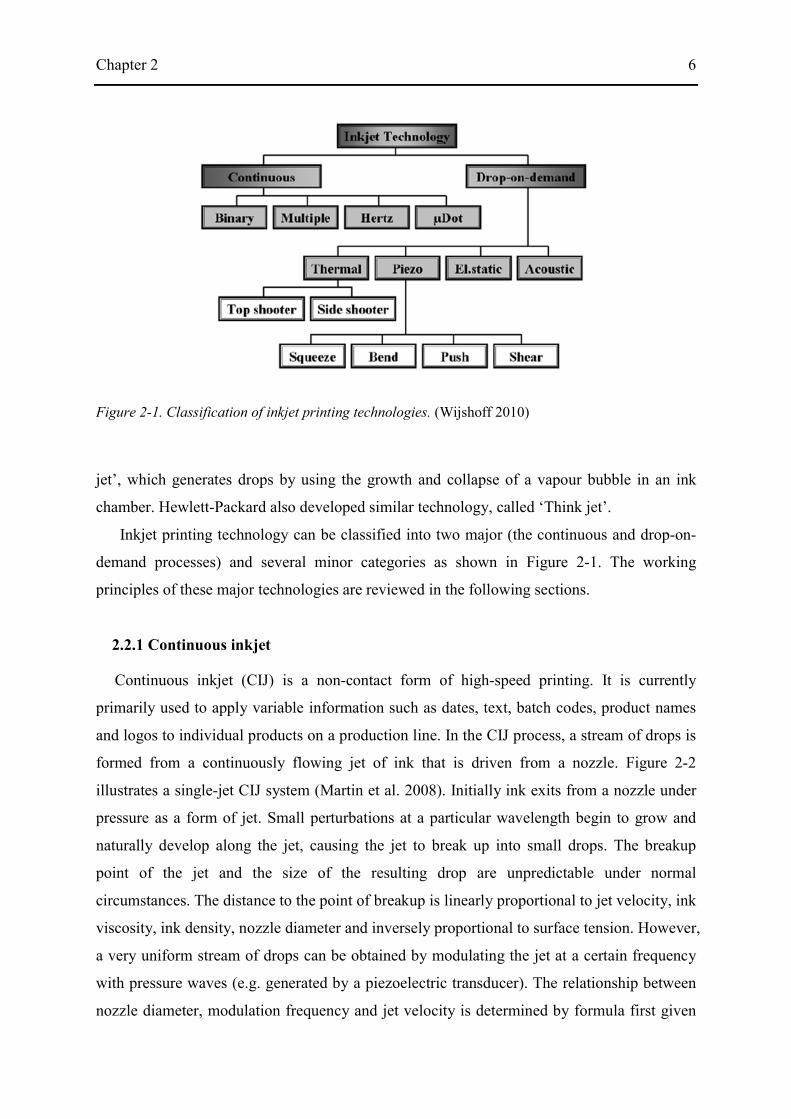
Inkjet printing technology can be classified into two major (the continuous and drop-on-
demand processes) and several minor categories as shown in Figure 2-1. The working
principles of these major technologies are reviewed in the following sections.
2.2.1 Continuous inkjet
Continuous inkjet (CIJ) is a non-contact form of high-speed printing. It is currently
primarily used to apply variable information such as dates, text, batch codes, product names
and logos to individual products on a production line. In the CIJ process, a stream of drops is
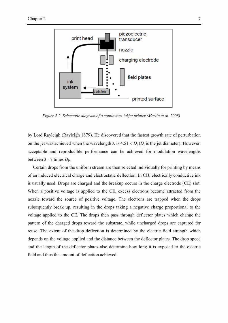
formed from a continuously flowing jet of ink that is driven from a nozzle. Figure 2-2
illustrates a single-jet CIJ system (Martin et al. 2008). Initially ink exits from a nozzle under
pressure as a form of jet. Small perturbations at a particular wavelength begin to grow and
naturally develop along the jet, causing the jet to break up into small drops. The breakup
point of the jet and the size of the resulting drop are unpredictable under normal
circumstances. The distance to the point of breakup is linearly proportional to jet velocity, ink
viscosity, ink density, nozzle diameter and inversely proportional to surface tension. However,
a very uniform stream of drops can be obtained by modulating the jet at a certain frequency
with pressure waves (e.g. generated by a piezoelectric transducer). The relationship between
nozzle diameter, modulation frequency and jet velocity is determined by formula first given
Figure 2-1. Classification of inkjet printing technologies. (Wijshoff 2010)
Chapter 2 7
by Lord Rayleigh (Rayleigh 1879). He discovered that the fastest growth rate of perturbation
on the jet was achieved when the wavelength λ is 4.51 × Dj (Dj is the jet diameter). However,
acceptable and reproducible performance can be achieved for modulation wavelengths
between 3 - 7 times Dj.
Certain drops from the uniform stream are then selected individually for printing by means
of an induced electrical charge and electrostatic deflection. In CIJ, electrically conductive ink
is usually used. Drops are charged and the breakup occurs in the charge electrode (CE) slot.
When a positive voltage is applied to the CE, excess electrons become attracted from the
nozzle toward the source of positive voltage. The electrons are trapped when the drops
subsequently break up, resulting in the drops taking a negative charge proportional to the
voltage applied to the CE. The drops then pass through deflector plates which change the
pattern of the charged drops toward the substrate, while uncharged drops are captured for
reuse. The extent of the drop deflection is determined by the electric field strength which
depends on the voltage applied and the distance between the deflector plates. The drop speed
and the length of the deflector plates also determine how long it is exposed to the electric
field and thus the amount of deflection achieved.
Figure 2-2. Schematic diagram of a continuous inkjet printer (Martin et al. 2008)
Chapter 2 8
2.2.2 Thermal inkjet
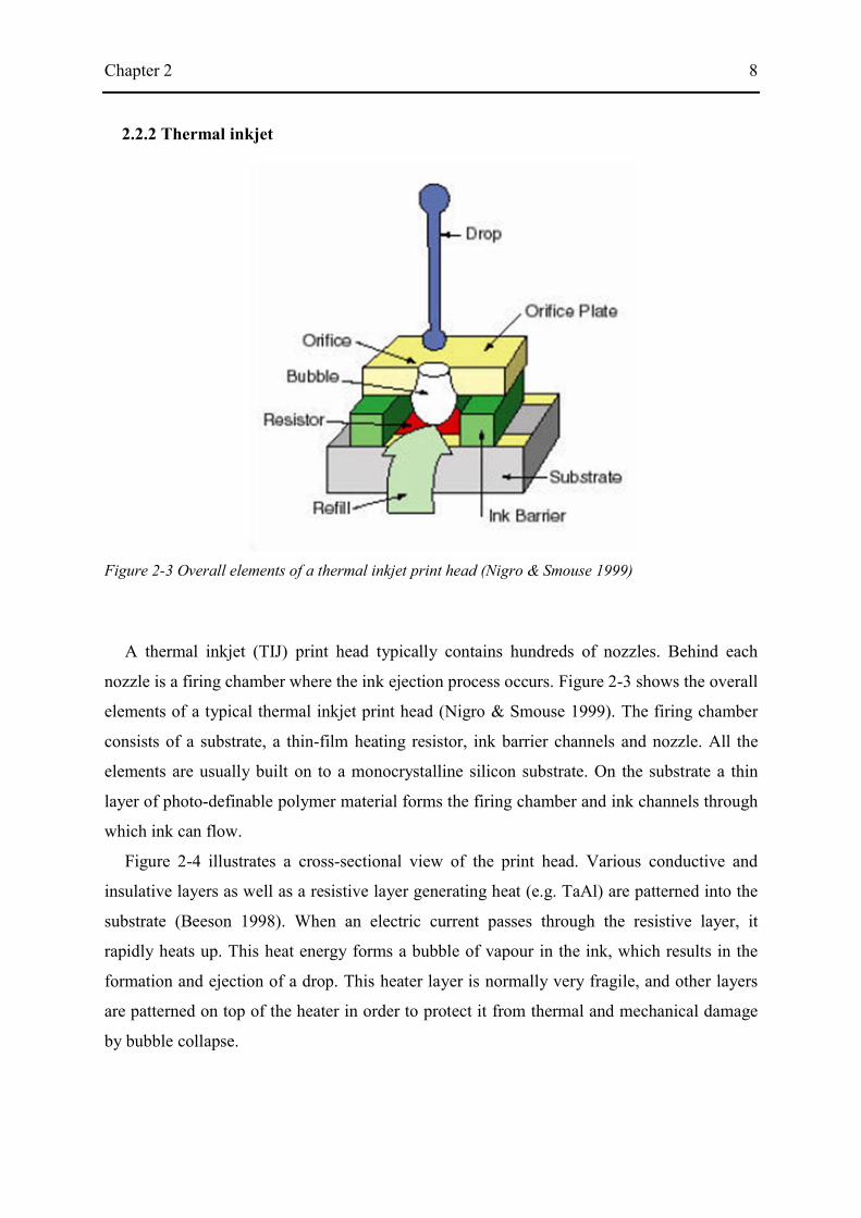
A thermal inkjet (TIJ) print head typically contains hundreds of nozzles. Behind each
nozzle is a firing chamber where the ink ejection process occurs. Figure 2-3 shows the overall
elements of a typical thermal inkjet print head (Nigro & Smouse 1999). The firing chamber
consists of a substrate, a thin-film heating resistor, ink barrier channels and nozzle. All the
elements are usually built on to a monocrystalline silicon substrate. On the substrate a thin
layer of photo-definable polymer material forms the firing chamber and ink channels through
which ink can flow.
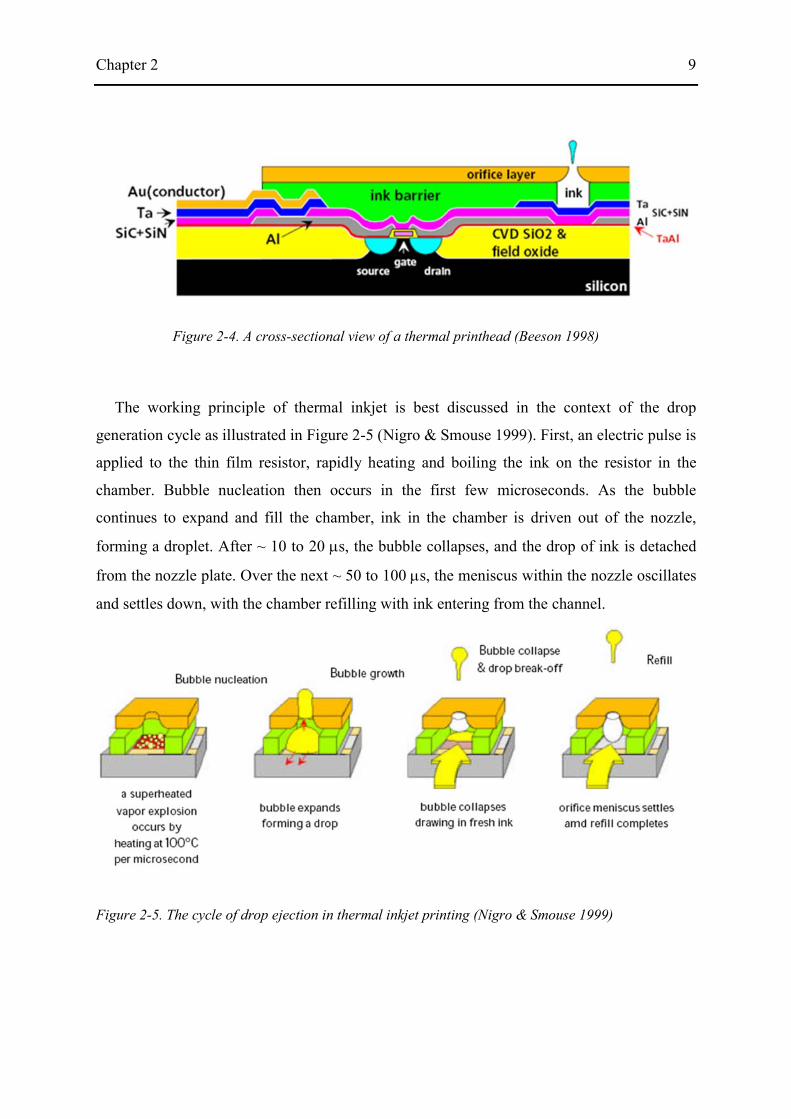
Figure 2-4 illustrates a cross-sectional view of the print head. Various conductive and
insulative layers as well as a resistive layer generating heat (e.g. TaAl) are patterned into the
substrate (Beeson 1998). When an electric current passes through the resistive layer, it
rapidly heats up. This heat energy forms a bubble of vapour in the ink, which results in the
formation and ejection of a drop. This heater layer is normally very fragile, and other layers
are patterned on top of the heater in order to protect it from thermal and mechanical damage
by bubble collapse.
Figure 2-3 Overall elements of a thermal inkjet print head (Nigro & Smouse 1999)
Chapter 2 9
The working principle of thermal inkjet is best discussed in the context of the drop
generation cycle as illustrated in Figure 2-5 (Nigro & Smouse 1999). First, an electric pulse is
applied to the thin film resistor, rapidly heating and boiling the ink on the resistor in the
chamber. Bubble nucleation then occurs in the first few microseconds. As the bubble
continues to expand and fill the chamber, ink in the chamber is driven out of the nozzle,
forming a droplet. After ~ 10 to 20 µs, the bubble collapses, and the drop of ink is detached
from the nozzle plate. Over the next ~ 50 to 100 µs, the meniscus within the nozzle oscillates
and settles down, with the chamber refilling with ink entering from the channel.
Figure 2-4. A cross-sectional view of a thermal printhead (Beeson 1998)
Figure 2-5. The cycle of drop ejection in thermal inkjet printing (Nigro & Smouse 1999)

Chapter 2 10
2.2.3 Piezoelectric inkjet
A piezoelectric inkjet (PIJ) print head, as the name implies, uses a piezoelectric material to
convert applied electrical energy into mechanical deformation of an ink chamber. The
displacement of the chamber wall generates the pressure required for a drop to form and eject
from the nozzle. Piezoelectric inkjet print head technologies are usually classified in terms of
the deformation mode used to generate the drop in Figure 2-6 (Brunahl 2002).
The squeeze mode PIJ was invented by Steven Zoltan in 1972 (US patent 3,683, 212,
1972). As shown in Figure 2-6(a), the actuator in this mode consists of a hollow tube of
piezoelectric material with electrodes on its inner and outer surface. The tube is radially
polarised, and this causes a contraction of the transducer when a driving voltage is applied.
The sudden displacement of the enclosed volume causes a drop of ink to be ejected from the
nozzle. Some of the ink is moved backward in the tube, but this is not significant because of
the high acoustic impedance of the long and narrow channel of the tube.
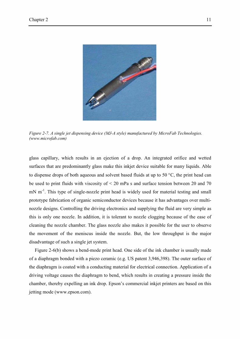
Figure 2-7 shows an example of a single jet dispensing device using the squeeze mode.
The print head consists of a glass capillary surrounded by a piezoelectric material. When an
electric voltage is applied to the piezoelectric material, it squeezes or expands the
Figure 2-6. Schematic diagrams of piezoelectric drop-on-demand inkjet technologies (Brunahl 2002)
Chapter 2 11
glass capillary, which results in an ejection of a drop. An integrated orifice and wetted
surfaces that are predominantly glass make this inkjet device suitable for many liquids. Able
to dispense drops of both aqueous and solvent based fluids at up to 50 °C, the print head can
be used to print fluids with viscosity of < 20 mPa s and surface tension between 20 and 70
mN m-1. This type of single-nozzle print head is widely used for material testing and small
prototype fabrication of organic semiconductor devices because it has advantages over multi-
nozzle designs. Controlling the driving electronics and supplying the fluid are very simple as
this is only one nozzle. In addition, it is tolerant to nozzle clogging because of the ease of
cleaning the nozzle chamber. The glass nozzle also makes it possible for the user to observe
the movement of the meniscus inside the nozzle. But, the low throughput is the major
disadvantage of such a single jet system.
Figure 2-6(b) shows a bend-mode print head. One side of the ink chamber is usually made
of a diaphragm bonded with a piezo ceramic (e.g. US patent 3,946,398). The outer surface of
the diaphragm is coated with a conducting material for electrical connection. Application of a
driving voltage causes the diaphragm to bend, which results in creating a pressure inside the
chamber, thereby expelling an ink drop. Epson’s commercial inkjet printers are based on this
jetting mode (www.epson.com).
Figure 2-7. A single jet dispensing device (MJ-A style) manufactured by MicroFab Technologies. (www.microfab.com)
Chapter 2 12
The push mode inkjet was invented by Stuart Howkins (US patent 4,459,601). As
illustrated in Figure 2-6(c), in this design a piezoelectric element pushes towards a wall of the
ink chamber to eject a drop. Although the actuator can directly push against the ink, a thin
diaphragm between the actuator and the ink is inserted to prevent unwanted interaction
between them. Trident is one of the companies developing inkjet print heads with this
technology (www.trident-itw.com).
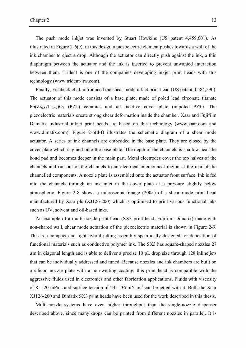
Finally, Fishbeck et al. introduced the shear mode inkjet print head (US patent 4,584,590).
The actuator of this mode consists of a base plate, made of poled lead zirconate titanate
Pb(Zr0.53Ti0.47)O3 (PZT) ceramics and an inactive cover plate (unpoled PZT). The
piezoelectric materials create strong shear deformation inside the chamber. Xaar and Fujifilm
Damatix industrial inkjet print heads are based on this technology (www.xaar.com and
www.dimatix.com). Figure 2-6(d-f) illustrates the schematic diagram of a shear mode
actuator. A series of ink channels are embedded in the base plate. They are closed by the
cover plate which is glued onto the base plate. The depth of the channels is shallow near the
bond pad and becomes deeper in the main part. Metal electrodes cover the top halves of the
channels and run out of the channels to an electrical interconnect region at the rear of the
channelled components. A nozzle plate is assembled onto the actuator front surface. Ink is fed
into the channels through an ink inlet in the cover plate at a pressure slightly below
atmospheric. Figure 2-8 shows a microscopic image (200×) of a shear mode print head
manufactured by Xaar plc (XJ126-200) which is optimised to print various functional inks
such as UV, solvent and oil-based inks.
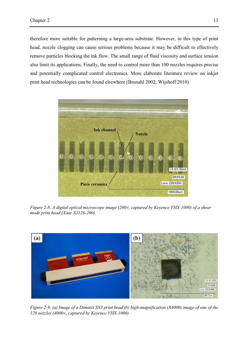
An example of a multi-nozzle print head (SX3 print head, Fujifilm Dimatix) made with
non-shared wall, shear mode actuation of the piezoelectric material is shown in Figure 2-9.
This is a compact and light hybrid jetting assembly specifically designed for deposition of
functional materials such as conductive polymer ink. The SX3 has square-shaped nozzles 27
µm in diagonal length and is able to deliver a precise 10 pL drop size through 128 inline jets
that can be individually addressed and tuned. Because nozzles and ink chambers are built on
a silicon nozzle plate with a non-wetting coating, this print head is compatible with the
aggressive fluids used in electronics and other fabrication applications. Fluids with viscosity
of 8 – 20 mPa s and surface tension of 24 – 36 mN m-1 can be jetted with it. Both the Xaar
XJ126-200 and Dimatix SX3 print heads have been used for the work described in this thesis.
Multi-nozzle systems have even higher throughput than the single-nozzle dispenser
described above, since many drops can be printed from different nozzles in parallel. It is
Chapter 2 13
therefore more suitable for patterning a large-area substrate. However, in this type of print
head, nozzle clogging can cause serious problems because it may be difficult to effectively
remove particles blocking the ink flow. The small range of fluid viscosity and surface tension
also limit its applications. Finally, the need to control more than 100 nozzles requires precise
and potentially complicated control electronics. More elaborate literature review on inkjet
print head technologies can be found elsewhere (Brunahl 2002; Wijshoff 2010)
Figure 2-8. A digital optical microscope image (200×, captured by Keyence VHX-1000) of a shear mode print head (Xaar XJ126-200).
Figure 2-9. (a) Image of a Dimatix SX3 print head (b) high-magnification (X4000) image of one of the 128 nozzles (4000×, captured by Keyence VHX-1000)
Chapter 2 14
2.3 Inkjet printing for organic semiconductor devices
Although inkjet printing technology has been widely used for both small-scale and large-
format graphical and text printing, it is now being increasingly considered to be a key
technology for fabricating plastic electronic devices. Examples of polymer inkjet printing
include the fabrication of polymer organic light-emitting diodes (P-OLEDs), organic thin film
transistors (OTFTs) and solar cells. Organic electronics are receiving much attention because
their manufacturing processes are far simpler than conventional silicon technology which
involves high-temperature and high-vacuum processes as well as very expensive plant. Inkjet
printing, as a material-conserving patterning method, can replace the complicated deposition
and lithographic patterning process involved in conventional silicon technology. The organic
electronics roadmap suggests that the organic and printed electronics market will exceed
$300 billion over the next 20 years (OE-A 2008). In this section, a brief overview is
presented on how inkjet printing has been used to fabricate organic electronic devices.
2.3.1 Polymer organic light-emitting diodes (P-OLEDs)
Plastic electronics evolved from fundamental work conducted in the field of molecular
electronics in the 1960s and ′70s. Electrical activity in plastic materials was first observed in
1977 when H. Shirakawa, A.G. Macdiarmid and A.J. Heeger, who were later awarded the
Nobel Prize for Chemistry, discovered that polymers could be made electrically conductive
after some modifications (Chiang et al. 1977; Shirakawa et al. 1977). They found that when
silvery films of the semiconducting polymer, polyacetylene were exposed to chlorine,
bromine or iodine, uptake of halogen occurs, and the conductivity increased dramatically by
over maximum seven orders of magnitude. In 1989, a research group led by Richard Friend at
the Cavendish laboratory of the University of Cambridge developed light emitting diodes
which were made from conducting polymers (Burroughes et al. 1990). Jeremy Burroughes, a
research student at that time, had been researching the applications of conducting polymers
when he noticed one sample was emitting a slight glow. “At first I thought it was the
reflection of the computer screen” Burroughs later commented “I turned it off to see if the
glow remained, and it did. I was absolutely amazed by this as it was something that was
supposed to be impossible.” (Seldon et al. 2003).
Since the startling discovery of organic electroluminescence from polymers in the
Cavendish Laboratory, P-OLEDs have received significant attention as the basis for the most
Chapter 2 15
promising next-generation flat panel displays. Compared to conventional displays such as
LED or Liquid-Crystal Display (LCD), the self-luminous display does not require a backlight
so that it can be thinner and lighter, consumes less energy, and can offer higher brightness
and contrast. Inkjet printing technology has been demonstrated to be well-suited to deposition
of light emitting polymer (LEP) solutions.
OLED substrates are typically patterned with an acrylate or polyimide photoresist in the
form of banks to define pixel wells into which the organic material is to be printed. Prior to
printing, the substrate is preconditioned in order to maximise wetting within the well and give
a non-wetting (low surface energy) surface to the photoresist bank in order to confine the
drying inks to within the pixel. In an ideal situation, ink completely fill the pixel well, such
that the ink pins at a point dependent only on the volume of ink, rather than other factors,
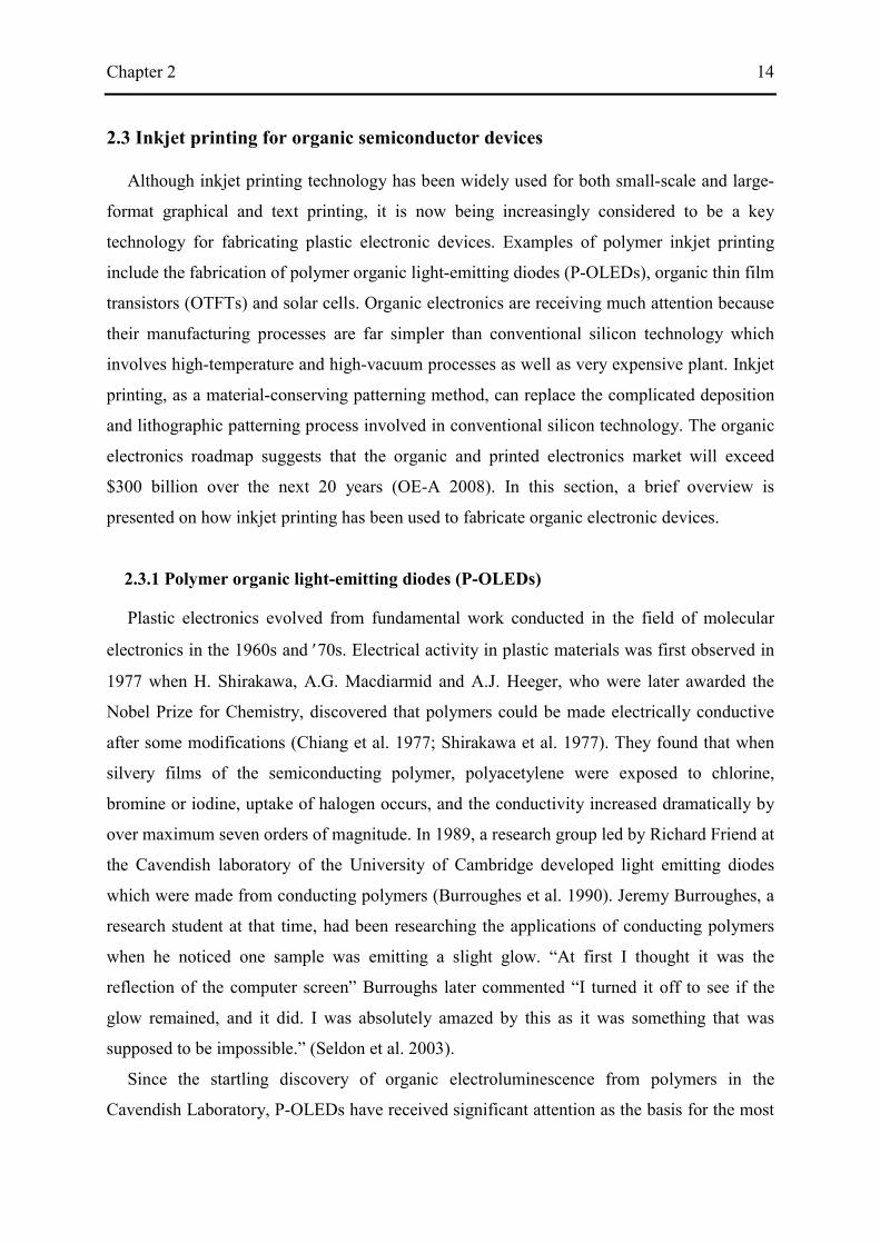
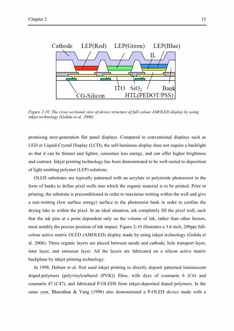
most notably the precise position of ink impact. Figure 2-10 illustrates a 3.6 inch, 200ppi full-
colour active matrix OLED (AMOLED) display made by using inkjet technology (Gohda et
al. 2006). Three organic layers are placed between anode and cathode; hole transport layer,
inter layer, and emission layer. All the layers are fabricated on a silicon active matrix
backplane by inkjet printing technology.
In 1998, Hebner et al. first used inkjet printing to directly deposit patterned luminescent
doped-polymers (polyvinylcarbazol (PVK)) films, with dyes of coumarin 6 (C6) and
coumarin 47 (C47), and fabricated P-OLEDS from inkjet-deposited doped polymers. In the
same year, Bharathan & Yang (1998) also demonstrated a P-OLED device made with a
Figure 2-10. The cross sectional view of device structure of full colour AMOLED display by using inkjet technology (Gohda et al. 2006).
Chapter 2 16
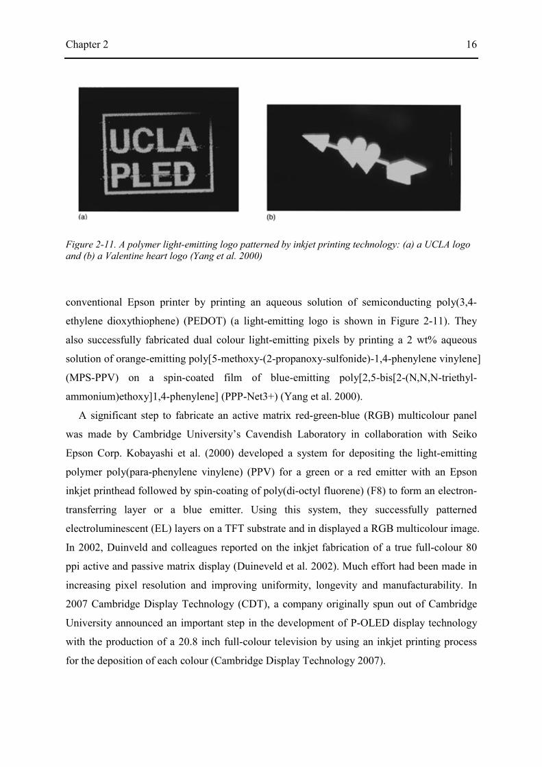
conventional Epson printer by printing an aqueous solution of semiconducting poly(3,4-
ethylene dioxythiophene) (PEDOT) (a light-emitting logo is shown in Figure 2-11). They
also successfully fabricated dual colour light-emitting pixels by printing a 2 wt% aqueous
solution of orange-emitting poly[5-methoxy-(2-propanoxy-sulfonide)-1,4-phenylene vinylene]
(MPS-PPV) on a spin-coated film of blue-emitting poly[2,5-bis[2-(N,N,N-triethyl-
ammonium)ethoxy]1,4-phenylene] (PPP-Net3+) (Yang et al. 2000).
A significant step to fabricate an active matrix red-green-blue (RGB) multicolour panel
was made by Cambridge University’s Cavendish Laboratory in collaboration with Seiko
Epson Corp. Kobayashi et al. (2000) developed a system for depositing the light-emitting
polymer poly(para-phenylene vinylene) (PPV) for a green or a red emitter with an Epson
inkjet printhead followed by spin-coating of poly(di-octyl fluorene) (F8) to form an electron-
transferring layer or a blue emitter. Using this system, they successfully patterned
electroluminescent (EL) layers on a TFT substrate and in displayed a RGB multicolour image.
In 2002, Duinveld and colleagues reported on the inkjet fabrication of a true full-colour 80
ppi active and passive matrix display (Duineveld et al. 2002). Much effort had been made in
increasing pixel resolution and improving uniformity, longevity and manufacturability. In
2007 Cambridge Display Technology (CDT), a company originally spun out of Cambridge
University announced an important step in the development of P-OLED display technology
with the production of a 20.8 inch full-colour television by using an inkjet printing process
for the deposition of each colour (Cambridge Display Technology 2007).
Figure 2-11. A polymer light-emitting logo patterned by inkjet printing technology: (a) a UCLA logo and (b) a Valentine heart logo (Yang et al. 2000)

Chapter 2 17
More recently, Singh et al. (2010) demonstrated bright inkjet-printed OLEDs based on Ir-
based phosphorescent macromolecules anchored on a polyhedral oligomeric silsesquioxane
(POSS) molecular scaffolding used as a phosphorescent dye in a polymer inkjet containing a
hole transporting polymer, poly(9-vinylcarbazole) and an electron transporting polymer, 2-4-
biphenylyl-5-4-tertburyl-phenly-1,3,4-oxadiazole (PBD). A peak luminance of more than
6000 cd m-2, a low turn-on voltage (6.8 V for 5 cd m-2) and a relatively high quantum
efficiency of 1.4 % were achieved in their research. Through improvement in dye chemistry
and print morphology, the authors were able to achieve a peak luminance of 10,000 cd m-2
(Figure 2-12). Wood et al. (2009) demonstrated a simple and scalable printing method to
achieve patterned pixels for flexible, full-colour, large-area, AC-driven displays operating at
video brightness. They showed that a quantum dot-polymer composite could be inkjet-printed
with stable ink solutions, and that it contributed to efficient and robust device architecture.
They also reported that inkjet printing technique was well-suited for integration with metal
oxide dielectric layers, which could enable improved optical and electrical performance.
Figure 2-12. Photograph of a 10,000 cd m-2 OLED printed using Ir-based polyhedral oligomeric silsesquioxane (POSS) macromolecules emitting at a peak wavelength of 520 nm (Singh et al. 2010).

Chapter 2 18
2.3.2 Polymer thin-film transistors
Organic thin film transistors (OTFT) have received much attention because their
fabrication processes are far less complex than conventional silicon or other inorganic
semiconductor technology. Field-effect transistors based on solution–processable organic
semiconductors have experienced impressive improvements in both performance and
reliability in recent years, particularly for the last ten years (Sirringhaus 2005a). Printing-
based manufacturing processes for integrated transistor circuits are being developed to realise
low-cost, large-area electronic products on flexible substrates. OTFTs have already been
demonstrated in applications such as electronic paper, sensors and memory devices including
radio frequency identification (RFID) tags (Reese et al. 2004).
One of the major obstacles to the development of organic transistors is in the achievable
minimum feature size by the inkjet printing process. The switching speed of a circuit relies on
mobility and the ratio between channel length and channel width of the transistor.
Commercial DoD inkjet printers can produce drops with a volume of some picoliters which
correspond to a drop diameter of typically 20–50 µm and a printing resolution of typically ≥
± 5 µm. The relatively poor resolution of the inkjet printing process limits the channel lengths
achievable in printed OTFTs to 10–100 µm, resulting in a very low and insufficient switching
speed of the transistor of 1–100 Hz (Zielke et al. 2005).
Figure 2-13. (left) Schematic diagram of high-resolution inkjet printing onto a pre-patterned substrate. (right) Atomic force microscopy (AFM) showing accurate alignment of inkjet printed PEDOT-PSS source and drain electrodes on a hydrophilic glass substrate, separated by a hydrophobic polyimide line with a channel length of 5 µm (Sirringhaus et al. 2000).

Chapter 2 19
Although inkjet printing had emerged as an attractive patterning technique for conjugated
polymers in OLED displays in the late 1990s, it had not been applied to organic transistors
until Sirringhaus and co-workers overcame this fundamental limitation in resolution in 2000
(Sirringhaus et al. 2000). They demonstrated direct inkjet printing of complete transistor
circuits, including via-hole interconnections based on solution-processed polymer conductors,
insulators and self-organising semiconductors. In their work, a non-wettable polyimide
pattern was defined by means of standard photolithography on a wettable glass substrate.
After the pre-treatment, they were able to deposit poly(3,4-ethylenedioxythiophene) doped
with polystyrene sulfonic acid (PEDOT/PSS) for the source-drain and gate electrode by using
a home-built, piezoelectric inkjet printer and achieved high-resolution definition with a
practical channel length of 5 µm (Figure 2-13).
Sekitani et al. (2008) demonstrated the feasibility of employing inkjet technology with
sub-femtoliter drop volume and single-micrometre resolution for electronic device
application. They fabricated p-channel and n-channel organic TFTs with source/drain
contacts prepared by sub-femtolitre inkjet printing of silver nanoparticles deposited directly
on to the surface of the organic semiconductor layers, without the need for any
photolithographic pre-patterning or any surface treatment.
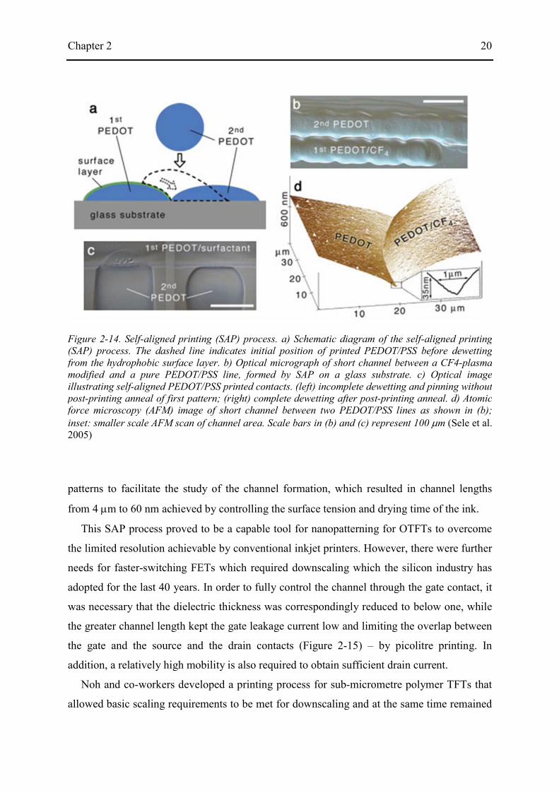
The Sirringhaus group further developed the additive printing technique for the
fabrication of OTFTs. In 2005 they announced a novel bottom-up, self-aligned inkjet printing
(SAP) process which was capable of defining sub-100nm critical features with two simple
additive printing steps using standard inkjet printing equipment without the need for any
lithography or precise relative alignment (Sele et al. 2005). The SAP technique comprises the
following three steps (Figure 2-14). 1) Patterning the first conductive polymer (PEDOT/PSS);
2) modifying the surface of the first pattern to be of low surface energy without modifying
the surface of the substrate; 3) printing a second conductive pattern such that it partially
overlaps the first conductive pattern. The droplets of the second pattern are repelled by and
flow off the low-energy surface of the first pattern and dry with their contact line in close
proximity to the edge of the first pattern, forming a small self-aligned gap. The typical
channel gap attained by this method was shorter than 100 nm.
The low conductivity of conductive polymer materials such as PEDOT/PSS is another
factor that limits the current flow in short-channel organic transistors. (Zhao et al. 2007)
extended the SAP printing method to the fabrication of functional conductive nanostructures
with gold nanoparticle ink. They printed the ink between two lithographically defined
Chapter 2 20
patterns to facilitate the study of the channel formation, which resulted in channel lengths
from 4 µm to 60 nm achieved by controlling the surface tension and drying time of the ink.
This SAP process proved to be a capable tool for nanopatterning for OTFTs to overcome
the limited resolution achievable by conventional inkjet printers. However, there were further
needs for faster-switching FETs which required downscaling which the silicon industry has
adopted for the last 40 years. In order to fully control the channel through the gate contact, it
was necessary that the dielectric thickness was correspondingly reduced to below one, while
the greater channel length kept the gate leakage current low and limiting the overlap between
the gate and the source and the drain contacts (Figure 2-15) – by picolitre printing. In
addition, a relatively high mobility is also required to obtain sufficient drain current.
Noh and co-workers developed a printing process for sub-micrometre polymer TFTs that
allowed basic scaling requirements to be met for downscaling and at the same time remained
Figure 2-14. Self-aligned printing (SAP) process. a) Schematic diagram of the self-aligned printing (SAP) process. The dashed line indicates initial position of printed PEDOT/PSS before dewetting from the hydrophobic surface layer. b) Optical micrograph of short channel between a CF4-plasma modified and a pure PEDOT/PSS line, formed by SAP on a glass substrate. c) Optical image illustrating self-aligned PEDOT/PSS printed contacts. (left) incomplete dewetting and pinning without post-printing anneal of first pattern; (right) complete dewetting after post-printing anneal. d) Atomic force microscopy (AFM) image of short channel between two PEDOT/PSS lines as shown in (b);inset: smaller scale AFM scan of channel area. Scale bars in (b) and (c) represent 100 µm (Sele et al. 2005)
Chapter 2 21
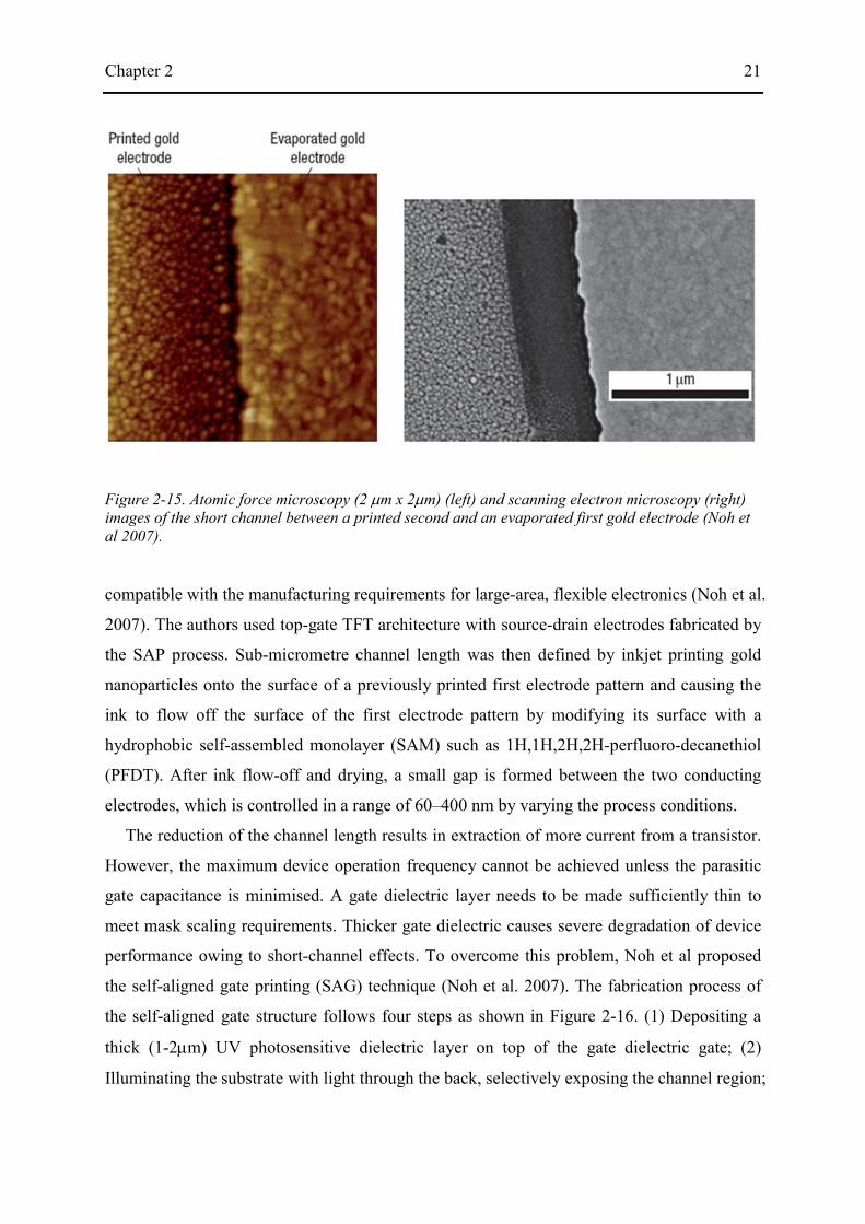
compatible with the manufacturing requirements for large-area, flexible electronics (Noh et al.
2007). The authors used top-gate TFT architecture with source-drain electrodes fabricated by
the SAP process. Sub-micrometre channel length was then defined by inkjet printing gold
nanoparticles onto the surface of a previously printed first electrode pattern and causing the
ink to flow off the surface of the first electrode pattern by modifying its surface with a
hydrophobic self-assembled monolayer (SAM) such as 1H,1H,2H,2H-perfluoro-decanethiol
(PFDT). After ink flow-off and drying, a small gap is formed between the two conducting
electrodes, which is controlled in a range of 60–400 nm by varying the process conditions.
The reduction of the channel length results in extraction of more current from a transistor.
However, the maximum device operation frequency cannot be achieved unless the parasitic
gate capacitance is minimised. A gate dielectric layer needs to be made sufficiently thin to
meet mask scaling requirements. Thicker gate dielectric causes severe degradation of device
performance owing to short-channel effects. To overcome this problem, Noh et al proposed
the self-aligned gate printing (SAG) technique (Noh et al. 2007). The fabrication process of
the self-aligned gate structure follows four steps as shown in Figure 2-16. (1) Depositing a
thick (1-2µm) UV photosensitive dielectric layer on top of the gate dielectric gate; (2)
Illuminating the substrate with light through the back, selectively exposing the channel region;
Figure 2-15. Atomic force microscopy (2 µm x 2µm) (left) and scanning electron microscopy (right) images of the short channel between a printed second and an evaporated first gold electrode (Noh et al 2007).

Chapter 2 22
(3) developing the photoresist to obtain a trench structure self-aligned to the edges of the
source and drain contacts; (4) inkjet printing a wide gate electrode with no need for precise
alignment. The SAG configuration minimised parasitic overlap capacitance to values as low
as 0.2-0.6 pF mm-1, and allowed transition frequencies of fT = 1.6 MHz to be reached.
Recently, a new T-shape configuration of electrodes was reported, based on single drop
contacts, which achieved a high device yield of 94-100% on arrays with very low leakage
current (Caironi et al. 2010). They also demonstrated that an inkjet printable silver-complex-
based ink, which can be sintered at low temperatures of 130°C to achieve near bulk silver
conductivity, is fully compatible with integration with organic semiconductors dielectrics.
This made it possible to fabricate organic semiconductors with a full solution-process,
without using any mask during the fabrication.
Most organic semiconductor devices developed so far have been unipolar (typically p-
type) and they have limitations in circuit integration because of low noise immunity and
relatively high power consumption. An attempt has been made to develop complementary
metal-oxide-semiconductor (CMOS) devices composed of both p-type and n-type FETs.
Baeg et al. first demonstrated inkjet-printed polymeric CMOS inverters and ring oscillators
which are key building blocks for digital and analogue integrated circuits. The inverters
exhibited high voltage gains (>30) and the five stage ring oscillators showed oscillator
frequencies approaching 50 kHz (Baeg et al. 2011). More information on this subject can be
found elsewhere (Sirringhaus 2005b; Klauk 2006)
Figure 2-16. Schematic diagram of the self-aligned gate (SAG) process: deposition of a photo-sensitive second dielectric on top of the semiconducting (SC) and gate dielectric (GD) layer and UV irradiation through the back of substrate; (b) development of the second dielectric to remove the exposed regions; (c) inkjet printing of gate electrode (Noh et al. 2007).
Chapter 2 23
2.3.3 Solar cells
A solar cell is a device which harnesses the sun’s ubiquitous energy to generate electricity
by means of the photovoltaic effect. A number of solar cells connected together form a solar
panel in order to generate useful electric power. Solar power is not yet widely utilised
because it involves more expensive materials, costlier processing methods and lower
efficiencies than fossil-fuel based energy sources (Singh et al. 2010). Initial organic-based
printed solar cells were successfully demonstrated in 2000 (Shaheen et al. 2001). In that work,
screen printing technology was used to fabricate bulk heterojunction plastic solar cells which
showed 4.3% power conversion efficiency when using an aluminium electrode and 488 nm
illumination. Marin and colleagues demonstrated inkjet printing of various electron
donor/acceptor compositions to build solar cells with bulk heterojunction structures on a
photoresist patterned glass substrate (Marin et al. 2005). Polymer:fullerene blends were
deposited by inkjet printing method for active layers of organic solar cells, achieving a power
conversion efficiency of 1.4% under simulated AM1.5 solar illumination (Aernouts et al.
2008).
Hoth et al. (2008) reported a record power conversion efficiency of 3.5% for inkjet printed
poly(3-hexylthlophene):fullerene based solar cells. They succeeded in their attempt to
properly control the nanomorphology of the polymer blend in the inkjet printing process by
adjusting the chemical properties of the poly(3-hexylthlophene) polymer donor. In the study
they discussed the correlation between material properties and the performance of the devices
fabricated with the inkjet printing patterning method. This morphology control of the
polymer blends still remains the core crucial issue to achieve higher performance in the
fabrication of solar cells (Chen et al. 2009). More recently, Eom et al. (2010) fabricated high
efficiency polymer solar cells by inkjet-printing both PEDOT:PSS and P3HT:PCBM (poly(3-
hexylthiophene) and 1-(3-methoxycarbonyl)-propyl-1-phenyl-(6,6)C61) layers. They found
that the addition of additives with high boiling points has significantly influenced the film
morphology, the optical and electrical properties and device performances. Apart from inkjet
printing process, a roll-to-roll printing process is also being used to make complete polymer
solar cell modules with no vacuum steps (Krebs 2009).
Although the present power conversion efficiency of solar cells is not sufficiently good for
commercial applications, they could revolutionise power generation if Moore’s law can be
applied to the capture of sunshine (Morton 2006).

Chapter 2 24
2.4 Collision of two impinging jets
Liquid atomisation from jets has been studied for industrial applications such as fuel
injection, liquid rocket engines, spray coating, and agrochemical spraying because of its high
efficiency and simple implementation (Villermaux 2007; Eggers & Villermaux 2008).
Experiments on the liquid sheets formed by the impact of two impinging jets were initially
performed by Savart while studying the cohesion of a liquid jet on a cylinder (Savart 1833).
G.I. Taylor studied the formation of sheets by the collision of laminar water jets, measured
the distribution of thickness in the sheets and compared the calculated shapes of the sheets
with photographs (Taylor 1960). Huang further developed Taylor’s work, examining the
break-up mechanism of the liquid sheet (Huang 2006). He reported three different break-up
regimes as a function of the jet Weber number. Dombrowski and Hooper investigated the
factors affecting the mechanism of disintegration of liquid sheets, and also studied how the
mean drop sizes varied with jet velocity and impact angle (Dombrowski 1963; Dombrowski
& Hooper 1964) . Over the last ten years, considerable attention has been paid by researchers
to sheet thickness, the distribution of liquid velocity and the shape of the liquid sheets formed
by obliquely colliding jets (Shen 1998; Choo & Kang 2002; Choo & Kang 2003; Li &
Ashgriz 2006; Clanet 2007) .
Heidmann et al. (1957) first reported the transition regime involving periodic atomisation
while studying sprays formed by two impinging jets of glycerol-water mixture to examine the
effect of discontinuities and variations in the flow of atomised propellants in rocket engines.
They speculated that such disintegration phenomena could originate either from unstable
equilibrium in the spray or from irregularities in the jets prior to impingement. While
considerable attention has been paid by subsequent researchers to sheet thickness, the
distribution of liquid velocity, and the shapes of the liquid sheets formed by colliding jets,
further aspects of the periodic atomisation pattern remained unexplored until Bush & Hasha
(2004) reported the results of a combined experimental and theoretical investigation of the
family of free-surface flows generated by symmetrical collision of two identical laminar jets.
For glycerol-water mixtures, they investigated the particular regime in which periodic
ligaments and droplets are formed as well as orthogonally linked sheets without drop
formation (the ‘fluid chain’). For the flow structure involving periodic atomisation, they used
the term ‘fluid fishbones’ because the shape, a long ‘spine’ from which a regular succession
of longitudinal ligaments and droplets emerged, was similar to that of a fish skeleton with the
Chapter 2 25
fluid sheet representing its head. More recently, Bremond & Villermaux (2006) studied the
formation and fragmentation of an ethanol sheet and demonstrated the formation of fishbone
structures in this system. In their work a sheet with periodic atomisation, which was rotated
so that the normal to the sheet lay at an angle to the plane containing the two jets, was
generated when a slight velocity difference existed between the two jets, whereas Bush &
Hasha (2004) reported the fishbone under conditions of symmetrical collision of two identical
jets.
Most previous work on colliding jets so far has been carried out with Newtonian fluids
(Dombrowski 1964; Bush & Hasha 2004; Huang 2006; Bremond & Villermaux 2006;
Bremond et al. 2007; Li & Ashgriz 2006; Villermaux 2007) . Few studies have used non-
Newtonian fluids, although it is known that the formation and subsequent break-up of a
continuous fluid stream from a nozzle is affected by elasticity and other non-Newtonian fluid
properties (Cooper-White et al. 2002; Bazilevskii et al. 2005). Miller et al. (2005) reported
experimental observations of fluid sheets formed by impinging laminar jets of worm-like
micelle solutions in which they found a new web-like flow structure. However, they did not
show the entire evolution of the flow structure as the velocity was increased and paid no
attention to periodic atomisation.
2.5 The drop impact process in inkjet printing
2.5.1 Drop impact process
The dynamics of a fluid drop impacting on a solid non-porous surface is a classical subject
of interfacial hydrodynamics, which occurs in many industrial and environmental situations
such as coating, rapid spray cooling of hot surfaces, quenching of aluminium alloys and steels,
motor jet, rain drop, pesticides and inkjet printing (Rein 1993; Yarin 2006). The impact of
liquid drops on dry surfaces creates various flow patterns depending on the properties of the
liquid and the surface. Liquids vary in density, viscosity, elasticity and surface tension. The
velocity and the size of a droplet also have a crucial influence on the resulting behaviours.
The solid surface may be rough or smooth, hydrophobic or hydrophilic, chemically
homogeneous or heterogeneous, planar or nonplanar, and normal or oblique. Rioboo et al.
(2001) identified six possible consequences of a droplet falling on to a dry surface: deposition,
Chapter 2 26
prompt splash, corona splash, receding break-up, partial rebound, and complete rebound as
seen in Figure 2-17.
Inkjet printing for organic semiconductor electronics involves the spreading of a liquid
drop on a smooth, dry, solid surface which can be described as a sequence of five successive
phases: kinematic, spreading, relaxation, wetting, and equilibrium (Rioboo et al. 2001).
Details of the drop’s behaviour depend on its impact speed, the liquid properties and the
surface wettability. As the drop collides with the surface, the initial shape of the region of the
drop which is out of contact remains largely unchanged in the initial (kinematic) stage. This
phase lasts approximately until the contact diameter reaches the original drop diameter. The
spreading phase then follows, in which the contact line expands radially and nearly all the
drop’s initial kinetic energy is consumed. The fluid properties and the impact conditions all
play a role in this phase. For example, higher impact speed or larger drop size lead to faster
spreading, whereas higher surface tension or viscosity results in slower expansion. After
spreading to a maximum extent, the drop may experience relaxation or oscillation of shape,
and possibly retraction of the contact line. A drop impacting on a hydrophobic surface may
Figure 2-17. A variety of morphologies of liquid drop impact on to a dry surface. (Rioboo et al. 2001)
Chapter 2 27
exhibit a receding contact line or even rebound if the initial kinetic energy is high enough;
rebound is common from super-hydrophobic surfaces. On the other hand, a drop on a
hydrophilic surface may oscillate or show a momentary pause in its expansion, and then
undergo further spontaneous spreading due to capillary effects until its size reaches a final
equilibrium state.
The extent to which drop wets the surface is usually described by its equilibrium contact
angle (θeq ), which is defined as the angle between the liquid/vapour interface as it meets the
solid surface (Figure 2-18). The liquid drop takes the shape which minimises the free energy
of the system, that is, minimising the surface area of the drop in the absence of gravity. Gibbs
demonstrated that minimising the free energy requires the minimisation of the sum (ψ) of
three energies contributed by the three interfaces (Starov et al. 2007)
ψ = σLFALF + σSLASL + σSFASF (2-1)
where σ is surface tension, A is area and the subscripts LF, SL, SF refer to liquid–fluid, solid–
liquid, solid–fluid interfaces, respectively. For a plane, homogeneous surface, the
minimisation yields,
LF
SLSF
σσσ
θ−
=cos (2-2)
This is known as Young’s equation. The wetting behaviour of a liquid drop according to the
contact angle is illustrated in Figure 2-19.
Figure 2-18. A liquid drop on a solid with an ideal contact angle (θ )
Chapter 2 28
In an ideal situation of a liquid spreading on a uniform plane solid, there is only one
equilibrium contact angle (θeq). But, in practice a number of stable angles can be measured
(Marmur 2006). Two relatively reproducible angles are the largest, called the ‘advancing
contact angle’ (θa) and the smallest called the ‘receding contact angle’ (θr). The advancing
angle can be measured by pushing the periphery of a drop over a surface and the receding
angle can be measured by pulling it back. The difference between the two angles (θa – θr) is
the contact angle hysteresis.
A substantial number of experimental, numerical and theoretical studies have been
conducted to identify the important parameters influencing the wetting process and the final
outcome of drop impact, for practical applications such as coating, painting, rapid spray
cooling of hot surfaces and the splat quenching of metallic alloys (De Gennes 1985; Daniel
Bonn et al. 2009). Many of these applications require a comprehensive understanding of the
wetting process (e.g. to predict how quickly a deposited drop will wet a given area of the
substrate). It is commonly reported that in the wetting stage the contact diameter D increases
slowly with time t according to a power law (‘Tanner’s law’):
D = ktn (2-3)
Figure 2-19. Wetting behaviour of a liquid drop according to the contact angle (θ )
Chapter 2 29
where the coefficient k depends on the competition between surface tension and viscosity
(Tanner 1979). The value of the index n has been shown to be ~0.1 both on theoretical
grounds and from experiments conducted with mm-sized drops (Tanner 1979; Lelah &
Marmur 1981; De Coninck et al. 2001).
With the further development of high-speed imaging techniques, researchers have also
been able to study the early stages of drop impact. These studies have attempted to quantify
the influence of the impact parameters and liquid properties, and to develop predictive
models (Kim & Chun 2001; Ukiwe & Kwok 2005; Yarin 2006; Attane et al. 2007; Yokoi et
al. 2008; Vadillo et al. 2009; Wang et al. 2009; Lee et al. 2010). While most of the earlier
experimental studies of drop impact were undertaken with mm-sized drops, the understanding
of the impact of much smaller drops (typically <100 µm in diameter) on to a dry solid surface
has grown in importance with the development of inkjet printing technology. Some studies of
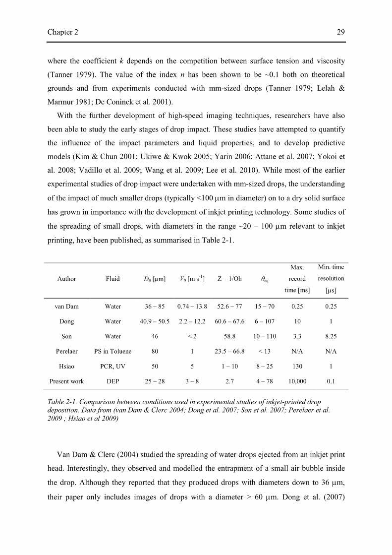
the spreading of small drops, with diameters in the range ~20 – 100 µm relevant to inkjet
printing, have been published, as summarised in Table 2-1.
Author Fluid D0 [µm] V0 [m s-1] Z = 1/Oh θeq
Max.
record
time [ms]
Min. time
resolution
[µs]
van Dam Water 36 – 85 0.74 – 13.8 52.6 – 77 15 – 70 0.25 0.25
Dong Water 40.9 – 50.5 2.2 – 12.2 60.6 – 67.6 6 – 107 10 1
Son Water 46 < 2 58.8 10 – 110 3.3 8.25
Perelaer PS in Toluene 80 1 23.5 – 66.8 < 13 N/A N/A
Hsiao PCR, UV 50 5 1 – 10 8 – 25 130 1
Present work DEP 25 – 28 3 – 8 2.7 4 – 78 10,000 0.1
Table 2-1. Comparison between conditions used in experimental studies of inkjet-printed drop deposition. Data from (van Dam & Clerc 2004; Dong et al. 2007; Son et al. 2007; Perelaer et al. 2009 ; Hsiao et al 2009)
Van Dam & Clerc (2004) studied the spreading of water drops ejected from an inkjet print
head. Interestingly, they observed and modelled the entrapment of a small air bubble inside
the drop. Although they reported that they produced drops with diameters down to 36 µm,
their paper only includes images of drops with a diameter > 60 µm. Dong et al. (2007)
Chapter 2 30
examined the impact of inkjet-printed drops (40 – 50 µm in diameter) on various smooth
solid substrates with different static contact angles (6° – 107°) at a wide range of speeds (2 –
12 m s-1) and studied the effects of impact speed and equilibrium contact angle θeq on the
time evolution of spreading diameter at the early stages (up to ~250 µs).
Son et al. (2008) explored the behaviour of drop spreading in the regime of low Weber
(We = ρDoVo2/σ) and Reynolds number (Re = ρDoVo/η) (0.05 < We < 2 and 10 < Re < 100).
Slowly falling water drops were deposited on to glass substrates which were treated by UV-
ozone plasma in order to vary their wettability. They presented images of deposited drops
from the impact phase to the equilibrium state, reporting that all the drops reached their
equilibrium state within 3.3 ms regardless of the equilibrium contact angle.
Perelaer et al. (2009) used solutions of polystyrene with molar masses between 1.5 and
545 kDa in toluene, with viscosities from 0.6 to 1.7 mPa s. They measured the diameter of
the drop after the solvent had evaporated, and found that it decreased with increasing
molecular weight of the polymer. Hsiao et al. (2009) investigated the spreading and wetting
dynamics of a printed drop particularly in the context of printed circuit board masking. Drops
of two commercial inks, a UV-curable ink and a phase-change resist (with melting
temperature of 70°C), were printed from an inkjet print head and imaged over a wide range of
time scales up to 200 ms. In their work, both flash-photography with a 20 ns spark light
source and continuous framing with a 27,000 fps high-speed camera were used to explore
early-stage impact-driven spreading and the later stage of wetting. However, their
experimental system did not effectively capture images of drops during the kinematic and
spreading phases which occurred in the first ~10 µs.
All these studies produced experimental results on the time evolution of the spreading
factor β (= D/Do), the ratio between the drop’s contact diameter on the surface D and its
original diameter Do, which could then be compared with predictive models. But
disagreements with the models were found in those papers, particularly for impact on to a low
contact-angle substrates, which are discussed in chapter 7. Analytical and empirical models
will also be reviewed in the next section.
It has been proposed that Z, the inverse of the Ohnesorge number (Oh), must lie in the
range Z > 2 (Fromm, 1984), which was later redefied by Reis and Derby (2000) who
predicted proper drop formation in the range 1 < Z < 10. Z is defined by Z = Re/ √We =
(ρσDo)1/2/η. Impact conditions with Z > 10, as used by several investigators, are not directly
Chapter 2 31
relevant to practical ink-jet printing. Only the work of Hsiao et al. (2009) has involved
appropriate jetting conditions (2 < Z < 3) with commercially-available inks. Some previous
studies used a single jet dispensing device, which can allow drops to be formed from a rather
wider range of fluids in terms of viscosity and surface tension. But commercially available
drop-on-demand (DOD) print heads for industrial applications typically require a narrower
range of fluid properties to achieve high performance, with viscosity of 7 – 20 mPa s and
surface tension of 20 – 40 mN m-1 in general.
Water, which has been used in some drop impact studies, has properties which are
markedly different from those of typical inks, with much higher surface tension and lower
viscosity (ρ ≈ 990 kg m-3, ρ ≈ 67 mN m-1 and η ≈ 1 mPa s). Toluene, as used by Perelaer et
al. (2009) also has very low viscosity (~ 0.5 mPa s). Drop impact speed is also important, and
in current practical drop-on-demand printing lies typically in the range from ~4 to ~8 m s-1 at
1 mm standoff distance (i.e. separation between printhead and substrate). Some previous
studies have been carried out at significantly lower speeds (Son et al. 2008; Perelaer et al.
2009).
Although most of works have focused on the drop impact process of Newtonian fluids so
far, the impact and spreading of non-Newtonian fluids on solid surfaces has also played a key
role in many fields of activities such as cooling, painting, food product, tablet coating and
pharmaceutical sprays. Understanding the spreading dynamics of a sub-100 µm low-
viscoelastic drop has grown in significance since inkjet printing is used as a patterning tool
for organic semiconductor devices. Unlike Newtonian fluids, the impact dynamics of a
viscoelastic fluid may be effectively controlled by its rheological properties as well as
viscosity or surface tension. But the spreading behaviour of a non-Newtonian fluid drop is
much less understood than those of a Newtonian drop. Particularly, the mechanism of an
inkjet-printed non-Newtonian drop impact on a wettable surface remains unknown to date.
Bergeron et al. (2000) first studied controlling drop deposition with polymer additives.
They discovered that drop rebound on a hydrophobic surface is markedly inhibited by adding
very small amounts of a PEO polymer to water. They argued that the non-Newtonian
elongational viscosity provided a large resistance to drop retraction after impact, thereby
suppressing drop rebound. But, the underlying physical mechanism at work still remains
controversial. Their explanation on the cause of the anti-rebound effect cannot explain why it
occurs only for the retraction phase and does not affect the spreading phase at all, because the
Chapter 2 32
elongational viscosity is dependent on the total deformation of the drop and thus should act in
the same way for both the spreading and retraction phase.
Bartolo et al. (2007) investigated the dynamics of non-Newtonian drops on hydrophobic
surfaces for polymeric solutions exhibiting strong normal stresses. They found that the
normal stresses resulting from the polymeric constitution of the drop fundamentally altered
the behaviour of the contact line and could considerably slow drop retraction. No noticeable
effects were observed during the expanding phase. More recently, Smith & Bertola (2010)
reported that bulk properties of the polymeric fluid played no role in the anti-rebound
phenomenon but the stretching of polymer chains produced an effective resistance to the
motion of the contact line.
Starov et al. (2003) theoretically investigated the wetting of non-Newtonian fluids on solid
substrates with the following assumption: (1) complete wetting; (2) a low dynamic contact
angle approximation; (3) a low non-Newtonian Reynolds number (Ren << 1); (4) The
dependency of the rheological properties of the fluid on shear deformation rate. They
proposed an explicit expression for the drop contour for both regimes of gravitational
spreading and capillary spreading and showed that a shear-thinning drop spreads more slowly
than an identical volume drop of corresponding Newtonian viscosity (i.e. the power-law
index of the Tanner’s law is less than 0.1).
All the studies mentioned above used 1-2 mm drops impacting at < 2 m s-1, and few
studies attempted to look at a sub-100 µm drop whose Newtonian and non-Newtonian fluid
properties and impact conditions lie within a practical inkjet printing regime. Recently, Son
& Kim (2009) experimentally studied the impact dynamics of non-Newtonian inkjet-printed
drop on solid substrates for the first time. They used PEO solutions in a mixture of water and
ethylene glycol (50:50 % by weight) with Oh << 1 and focused on the polymer effect on
impact dynamics for a relaxation phase over 20 – 140 µs after impact with a high-speed
camera at the frame rate of 100,000 fps. They found that distinct difference between the
Newtonian solvent and non-Newtonian solutions lay in their oscillation motion during the
relaxation phase with the viscoelastic solutions taking longer time in oscillation. Perelaer et al.
(2009) reported that the diameter of a dried liquid film of a polystyrene solution in toluene
diameter decreased with increasing molecular weight of the polymer due to increase in low-
shear viscosity.

Chapter 2 33
2.5.2 Models for the prediction of maximum drop spreading
A model to predict the maximum spreading diameter can be derived from the energy
conservation equation, the mass and momentum equations or the lubrication approximation
equation. Energy conservation has been used most widely because of its simplicity and the
ability to produce an analytical equation. This approach is based on the fact that the sum of
the kinetic, gravitational and surface energies, EK1, EG1, Es1 of the drop at impact must be
equal to the sum of the kinetic energy, gravitational energy, surface energy and energy lost in
viscous dissipation EK2, EG2, Es2, ED2 for the spreading drop:
EK1 + EG1 + Es1 = EK2 + EG2 + Es2 + ED2 (2-4)
If the drop reaches its maximum diameter at the end of the spreading phase, before the
relaxation or oscillation phase, then the kinetic energy of the drop (EK2) momentarily
becomes zero. Since the contribution of the gravitational energy is negligible for a very small
drop, the equation then becomes:
EK1 + Es1 = Es2 + ED2 (2-5)
Some analytical models based on this relationship are reviewed below.
Early models were developed for the impact of a molten-metal drop on to a cool substrate.
In these models the maximum spreading diameter was considered to be the final diameter of
the drop. Jones developed a simple model for the cooling and freezing of Al-Fe alloy drops
generated by rotary atomisation (Jones 1971). He assumed that the contribution of surface
energy to the termination of drop spreading was negligible, which led to the result that the
maximum diameter was proportional to Re1/8. Madejski (1976)studied the solidification of
molten alumina drops generated in plasma spraying, for Re > 100 and We > 100. His model
systematically accounted for viscous dissipation, surface tension effects and simultaneous
freezing of the splat. Collings et al. (1990) modelled the splat-quench solidification of a
freely falling liquid drop, and predicted an upper bound on the final splat diameter (in terms
of the maximum spreading factor β*) by neglecting viscous energy dissipation, as follows:
2/1
)cos1(312We*
−+
=eqθ
β (2-6)
Chapter 2 34
where θeq is the equilibrium contact angle between the liquid and the solid surface. These
models have been reviewed elsewhere (Bennett & Poulikakos 1993)
Chandra & Avedisian (1991) studied the impact of a n-heptane drop on to a solid metallic
surface. Surface temperature was varied between 24 °C and 200 °C, which had a marked
effect on the contact angle which varied from 32° to 180°. Unlike in previous models for
molten metal impact, they considered the maximum diameter of the liquid sheet at the end of
the first expansion phase, rather than the final contact diameter, because in their work the
drops experienced significant recoil and rebound from the heated surface which is not
generally observed in drop impact involving solidification. They took into account kinetic
energy, surface energy and viscous dissipation, and their model showed reasonably good
agreement with experimental results, with errors of about 20%. Their model has been widely
used. Pasandideh-Fard et al. (1996) modified it by using the advancing contact angle (θa) to
calculate surface energy at the point of maximum contact diameter, and also used the speed
profile of stagnation-point flow for the calculation of viscous dissipation. They showed that:
2/1
Re/We4)cos1(312We*
+−+
=aθ
β (2-7)
Park et al. (2003) and Ukiwe et al. (2005) developed the model of (Pasandideh-Fard et al.
1996) further. Park et al. (2003) assumed that at the point of maximum spreading the drop
takes the form of a truncated sphere rather than a cylindrical disk. In addition, they took
account of the decrease in surface and interfacial energies for spontaneous spreading from the
impact phase to the spreading phase, and derived the following expression:
2/13/233
Re/We4)cos(3
)])coscos32/(sin4(cos[312We*
+−
+−−++=
eqs
eqeqeqeqs
f
f
θ
θθθθβ
(2-8)
where d
dsf
θθ
2sin)cos1(2 −
=
This increased the accuracy of the diameter prediction, despite the fact that a cylindrical
disk shape at the point of maximum spreading had been widely observed (Chandra &
Avedisian 1991; Ukiwe & Kwok 2005). But this model has the disadvantage that it requires a
Chapter 2 35
value for the dynamic contact angle at maximum spreading, θd, which must be measured
experimentally.
Ukiwe et al. studied the impact of water drops at a fixed Weber number of 59 on to solid
surfaces (Ukiwe et al. 2005). They modified Pasandideh-Fard’s model (1996) and obtained
better agreement with their experimental results for maximum spreading diameter by
considering an additional surface energy term at the point of maximum spreading. In addition,
they replaced the advancing contact angle by the equilibrium angle (Marmur 2006) . Their
expression was:
2/1
Re/We4)cos1(3*/812We*
+−−+
=eqθ
ββ (2-9)
Roisman et al. (2002) used the mass and momentum equations and incorporated the
effects of inertial, viscous and surface forces, and wettability. They developed a simplified
approximation to predicting the maximum spreading diameter for Re >> We (i.e. where the
viscous contribution can be neglected). They used the lubrication approximation equation to
study the spreading of drops on partially or completely wettable surfaces, but did not produce
a simple analytical equation for β∗ (Clay & Miksis 2004). Semi-empirical and empirical
models for liquid drop impact on to a solid, dry surface can also be found elsewhere.
It should be noted that the maximum spreading factor β* predicted by the models
described above does not necessarily involve the final equilibrium diameter of the drop. As
Rein has pointed out, the maximum spreading factor should be defined in terms of the
maximum diameter at the end of spreading phase, D*, at the point where the kinetic energy
momentarily becomes zero, and not the final value of the diameter at the end of the whole
impact process, D∞ (Rein 1993). Figure 2-20 illustrates possible curves for the time evolution
of β, for two surfaces with differing wettability. The value of the maximum spreading factor
can be readily determined for spreading on a non-wettable surface (b) because β∗ is equal to
or greater than β∞ in those cases. For a highly wettable surface (a), however, the value of
β∞ tends to be larger than β∗ and there is potential for confusion as to the meaning of the term
‘maximum’ spreading factor. For clarity, we here define the maximum spreading factor at the
end of the initial spreading phase to be β∗, rather than βmax as has commonly been used in the
previous literature, and the final, equilibrium spreading factor to be β∞.

Chapter 2 36
As discussed above, various models for β∗ have been proposed. The equilibrium
spreading factor β∞ can be readily predicted from volume conservation, from the assumption
that the final drop forms a spherical cap in its equilibrium state (van Dam & Clerc 2004). A
unique value for β∞ is then determined from a knowledge of the static contact angle θeq:
3/1
2 )]2/(tan3)[2/tan(8
+=∞
eqeq θθβ
(2-10)
In contrast, it is clearly not appropriate to attempt to predict β∗ from volume conservation,
because at the point of maximum spreading the drop will normally have the shape of a
flattened disk rather than a spherical cap, and also because the dynamic contact angle at that
point will be quite different from the static contact angle applicable at the end of the wetting
phase.
Figure 2-20. Schematic illustration of the evolution of the spreading factor (β) as a function of dimensionless time (τ) for drops impacting on three surfaces with different wettability. The maximum spreading factor (β*) and the dimensionless time to reach β* (τ*) as well as the final spreading factor (β∞) and dimensionless time to reach β∞ (τ∞) for a highly wettable surface are indicated. The two curves correspond to: (a)β*<β∞ (highly wettable surface); (b) β*>β∞ (non-wettable surface)
Chapter 2 37
2.6 High–speed imaging techniques
Development of full understanding of the drop impact dynamics on a solid surface is
critically dependent on the capturing of clear images of a deformed drop as it impacts and
spreads on the surface. The initial phases of the impact process occur over a very short period,
generally in a few milliseconds for a millimetre size droplet and several microseconds for a
sub–100 µm droplet, while the drop can further experience an extended wetting process for
more than a second. This implies that for the study of the impact dynamics of an inkjet-
printed drop a high-speed camera with both a very short exposure time and a temporal
resolution of << 1 µs is essential to freeze the droplet’s image during different phases while it
impacts. The earliest successful attempts were made by Worthington (Worthington 1876)
who observed the patterns made by a liquid droplet during impact on a glass surface. His
observation depended on direct observation with the naked eye while illumination by an
electric spark with a very short exposure time froze the image. Since then, high-speed
imaging has been developed and applied to investigate drop impact dynamics in two ways:
cinematography and flash-photography.
2.6.1 Cinematography
High-speed cinematography is a photographic method to record successive pictures with
adequately short exposures and fast enough framing rates (more than 1000 frames per second
in general) for an event to be evaluated (Ray 1997). Since the middle of the twentieth century
this method has been applied to record the drop impact process. The quality of the published
images, unfortunately, is generally not clear enough to discern different phases of the impact
process. However, since the launch of the Kodak high speed motion analyser in 1986
significant improvement in image quality has been achieved. The Kodak Ektapro 1000/2000
motion analyser achieved a frame rate of 1000 − 2000 per second. The images stored in the
digital memory of the camera were transferred to a video tape for further analysis. As
examples, Kim & Chun (2001) employed the high-speed Kodak imaging system to inspect
the recoil of mm-sized liquid drops and the impact of drops onto various solid substrates.
More recently, Son et al. (2008) used a high-speed camera (Redlake, MotionPro X-4) to take
impact images of sub-100 µm drops. Typical images are shown in Figure 2-21.

Chapter 2 38
In 1991 Photron launched the world's fastest commercial high-speed video system,
operating at up to 40,500 frames per second. This new digital video technology allowed a
user to access the image data immediately, eliminating the step of copying on to an analogue
video tape. Such high-speed cameras can be applied to study the impact dynamics of a
millimetre size droplet with velocity of 1 to 2 m s-1. It takes from hundreds of milliseconds to
several seconds for the droplet to reach its equilibrium phase after colliding with a surface.
As a light source, a continuous light is suitable for obtaining discernible images. The shutter
speed of the camera can be adjustable over a range from tens of microseconds to tens of
milliseconds by increasing the frame rate. But the higher frame rate results in reduced image
size, lowering the image resolution and shortening the recording period. Replacing the
continuous light with a stroboscope makes it possible to obtain better quality images at lower
frame rate without reducing the image size. In this regime the exposure time is determined
not by the shutter speed but by the duration of the stroboscope flash which can be shorter
than that of the shutter speed. Precise synchronisation is needed between the light source and
the camera to achieve good images. The types of possible light source and their duration are
Figure 2-21. Sequential images of drop impact taken by high-speed cameras. (a) 4 mm-sized water drop (Kim and Chun 2001); (b) 46 µm-sized water drop (Son et al. 2008).
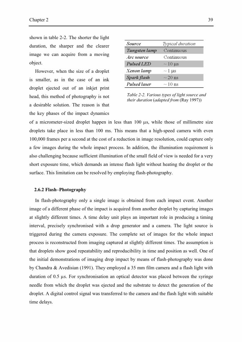
Chapter 2 39
shown in table 2-2. The shorter the light
duration, the sharper and the clearer
image we can acquire from a moving
object.
However, when the size of a droplet
is smaller, as in the case of an ink
droplet ejected out of an inkjet print
head, this method of photography is not
a desirable solution. The reason is that
the key phases of the impact dynamics
of a micrometer-sized droplet happen in less than 100 µs, while those of millimetre size
droplets take place in less than 100 ms. This means that a high-speed camera with even
100,000 frames per a second at the cost of a reduction in image resolution, could capture only
a few images during the whole impact process. In addition, the illumination requirement is
also challenging because sufficient illumination of the small field of view is needed for a very
short exposure time, which demands an intense flash light without heating the droplet or the
surface. This limitation can be resolved by employing flash-photography.
2.6.2 Flash–Photography
In flash-photography only a single image is obtained from each impact event. Another
image of a different phase of the impact is acquired from another droplet by capturing images
at slightly different times. A time delay unit plays an important role in producing a timing
interval, precisely synchronised with a drop generator and a camera. The light source is
triggered during the camera exposure. The complete set of images for the whole impact
process is reconstructed from imaging captured at slightly different times. The assumption is
that droplets show good repeatability and reproducibility in time and position as well. One of
the initial demonstrations of imaging drop impact by means of flash-photography was done
by Chandra & Avedisian (1991). They employed a 35 mm film camera and a flash light with
duration of 0.5 µs. For synchronisation an optical detector was placed between the syringe
needle from which the droplet was ejected and the substrate to detect the generation of the
droplet. A digital control signal was transferred to the camera and the flash light with suitable
time delays.
Table 2-2. Various types of light source and their duration (adapted from (Ray 1997))
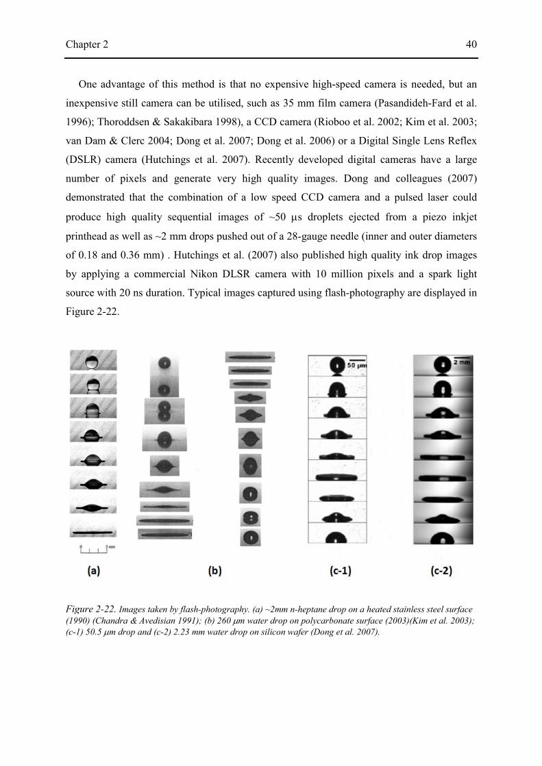
Chapter 2 40
One advantage of this method is that no expensive high-speed camera is needed, but an
inexpensive still camera can be utilised, such as 35 mm film camera (Pasandideh-Fard et al.
1996); Thoroddsen & Sakakibara 1998), a CCD camera (Rioboo et al. 2002; Kim et al. 2003;
van Dam & Clerc 2004; Dong et al. 2007; Dong et al. 2006) or a Digital Single Lens Reflex
(DSLR) camera (Hutchings et al. 2007). Recently developed digital cameras have a large
number of pixels and generate very high quality images. Dong and colleagues (2007)
demonstrated that the combination of a low speed CCD camera and a pulsed laser could
produce high quality sequential images of ~50 µs droplets ejected from a piezo inkjet
printhead as well as ~2 mm drops pushed out of a 28-gauge needle (inner and outer diameters
of 0.18 and 0.36 mm) . Hutchings et al. (2007) also published high quality ink drop images
by applying a commercial Nikon DLSR camera with 10 million pixels and a spark light
source with 20 ns duration. Typical images captured using flash-photography are displayed in
Figure 2-22.
Figure 2-22. Images taken by flash-photography. (a) ~2mm n-heptane drop on a heated stainless steel surface (1990) (Chandra & Avedisian 1991); (b) 260 µm water drop on polycarbonate surface (2003)(Kim et al. 2003); (c-1) 50.5 µm drop and (c-2) 2.23 mm water drop on silicon wafer (Dong et al. 2007).

Chapter 3 41
3. Fluid characterisation
3.1 Introduction
This chapter provides the background to various methods for characterising viscoelastic
fluids. Section 3.2 explains some background knowledge on viscoelasticity such as viscous
and elastic modulus. A recently developed high-frequency rheometer and filament stretching
rheometer as well as a conventional rotational rheometer are in section 3.3. Then section 3.4
introduces dimensionless groups for the systematic understanding of the various forces
involved in drop impact processes.
3.2 Viscoelasticity
Viscoelasticity is a property of materials that exhibit both viscous and elastic behaviours
when undergoing deformation (Wissbrun 1999). It is not only related to the total amount of
deformation but also to its rate. For Newtonian fluids such as water, air and low molecular
weight liquids, their viscosity (η) is constant and shear stress (τs) is directly proportional to
shear rate (��).
�� = ��� (3-1)
Any fluid that does not obey the Newtonian relationship between the shear stress and
shear rate is classified into non–Newtonian. For example, high molecular weight liquids
including polymer melts and solutions of polymers are usually non-Newtonian. In this case,
the shear stress does not have a linear relationship with the shear rate.
The viscosity of a typical molten polymer has a constant value ηο called the zero (or low)
shear viscosity at sufficiently low shear rates. But, the viscosity monotonically decreases as
the shear rate increases, showing shear thinning behaviour as shown Figure 3-1(a). Here, the
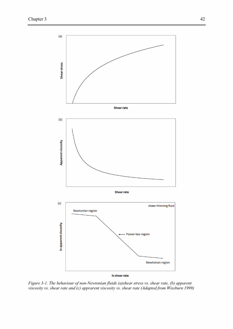
Chapter 3 42
Figure 3-1. The behaviour of non-Newtonian fluids (a)shear stress vs. shear rate, (b) apparent viscosity vs. shear rate and (c) apprarent viscosity vs. shear rate (Adapted from Wissburn 1999)
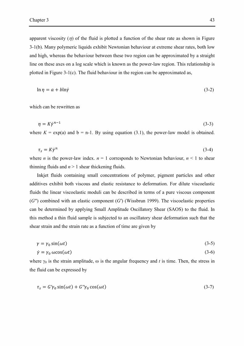
Chapter 3 43
apparent viscosity (η) of the fluid is plotted a function of the shear rate as shown in Figure
3-1(b). Many polymeric liquids exhibit Newtonian behaviour at extreme shear rates, both low
and high, whereas the behaviour between these two region can be approximated by a straight
line on these axes on a log scale which is known as the power-law region. This relationship is
plotted in Figure 3-1(c). The fluid behaviour in the region can be approximated as,
ln � = � + �ln�� (3-2)
which can be rewritten as
� = ��� ��� (3-3)
where K = exp(a) and b = n-1. By using equation (3.1), the power-law model is obtained.
�� = ��� � (3-4)
where n is the power-law index. n = 1 corresponds to Newtonian behaviour, n < 1 to shear
thinning fluids and n > 1 shear thickening fluids.
Inkjet fluids containing small concentrations of polymer, pigment particles and other
additives exhibit both viscous and elastic resistance to deformation. For dilute viscoelastic
fluids the linear viscoelastic moduli can be described in terms of a pure viscous component
(G′′) combined with an elastic component (G′) (Wissbrun 1999). The viscoelastic properties
can be determined by applying Small Amplitude Oscillatory Shear (SAOS) to the fluid. In
this method a thin fluid sample is subjected to an oscillatory shear deformation such that the
shear strain and the strain rate as a function of time are given by
� = �� sin(��) (3-5)
�� = �� ωcos(��) (3-6)
where γ0 is the strain amplitude, ω is the angular frequency and t is time. Then, the stress in
the fluid can be expressed by
�� = �′�� sin(��) + �′′�� cos(��) (3-7)

Chapter 3 44
The first term is in-phase with the strain rate and the second term is out-of-phase. It is
convenient to think of G′ and G′′ as the real and imaginary components, respectively, of a
complex modulus (G*) defined as follows:
ωη /*)( 2''2'* =+= GGG (3-8)
where η* is the complex viscosity. The elasticity ratio G′/|G*|, which is calculated from the
equations above, can be used to indicate the relative elastic component of the viscoelastic
response of the fluid.
The behaviours of many viscoelastic fluids can be generalised by a mechanical single-
mode Maxwell model, which consists of a spring in parallel with a dashpot. In this model, the
spring represents a linear elastic element, in which the force applied is proportional to the
extension. On the other hand, the dashpot represents the purely viscous component of the
response, in which the force linearly increases with the rate of the extension. For this model,
G′ and G′′ can be shown to be given by:
2
2'
)(1)(
ωλωλ
+=
GG (3-9)
20''
)(1 ωλωλωη
++=
GG (3-10)
where G is the spring constant, and λ is the relaxation time. In the low frequency limit, they
can be simplified to:
22
2' )(
)(1)( ωλ
ωλωλ GGG ≈
+= (3-11)
)()(1 020
'' ληωωλωλωη GGG +≈
++= (3-12)
Therefore, for a fluid which obey the Maxwell model the frequency dependencies of G′ and
G'′ should follow power-law exponents of 2 for G′ and 1 for G'′, as shown by equations (3-11)
and (3-12).
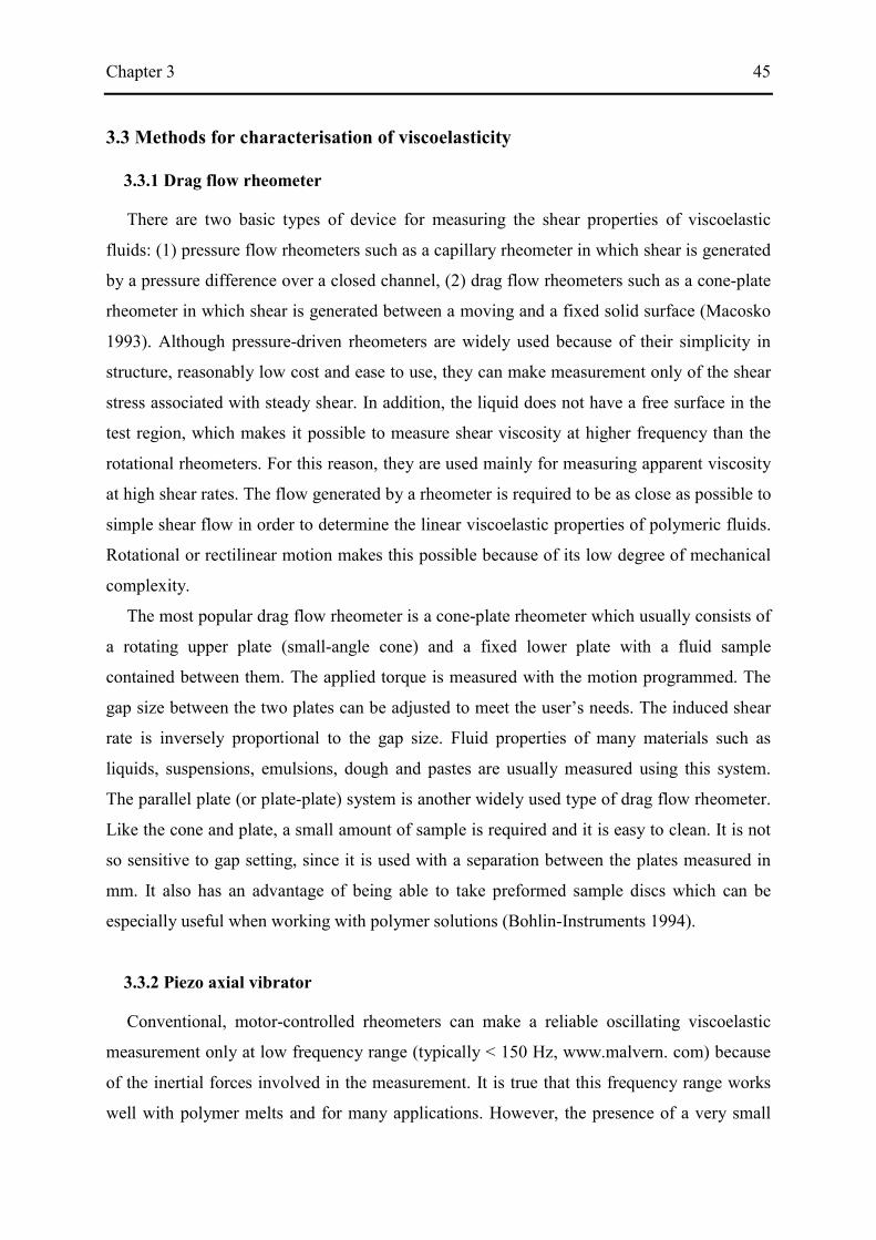
Chapter 3 45
3.3 Methods for characterisation of viscoelasticity
3.3.1 Drag flow rheometer
There are two basic types of device for measuring the shear properties of viscoelastic
fluids: (1) pressure flow rheometers such as a capillary rheometer in which shear is generated
by a pressure difference over a closed channel, (2) drag flow rheometers such as a cone-plate
rheometer in which shear is generated between a moving and a fixed solid surface (Macosko
1993). Although pressure-driven rheometers are widely used because of their simplicity in
structure, reasonably low cost and ease to use, they can make measurement only of the shear
stress associated with steady shear. In addition, the liquid does not have a free surface in the
test region, which makes it possible to measure shear viscosity at higher frequency than the
rotational rheometers. For this reason, they are used mainly for measuring apparent viscosity
at high shear rates. The flow generated by a rheometer is required to be as close as possible to
simple shear flow in order to determine the linear viscoelastic properties of polymeric fluids.
Rotational or rectilinear motion makes this possible because of its low degree of mechanical
complexity.
The most popular drag flow rheometer is a cone-plate rheometer which usually consists of
a rotating upper plate (small-angle cone) and a fixed lower plate with a fluid sample
contained between them. The applied torque is measured with the motion programmed. The
gap size between the two plates can be adjusted to meet the user’s needs. The induced shear
rate is inversely proportional to the gap size. Fluid properties of many materials such as
liquids, suspensions, emulsions, dough and pastes are usually measured using this system.
The parallel plate (or plate-plate) system is another widely used type of drag flow rheometer.
Like the cone and plate, a small amount of sample is required and it is easy to clean. It is not
so sensitive to gap setting, since it is used with a separation between the plates measured in
mm. It also has an advantage of being able to take preformed sample discs which can be
especially useful when working with polymer solutions (Bohlin-Instruments 1994).
3.3.2 Piezo axial vibrator
Conventional, motor-controlled rheometers can make a reliable oscillating viscoelastic
measurement only at low frequency range (typically < 150 Hz, www.malvern. com) because
of the inertial forces involved in the measurement. It is true that this frequency range works
well with polymer melts and for many applications. However, the presence of a very small

Chapter 3 46
concentration of polymer can significantly influence the performance of inkjet printing
(Bazilevskii et al. 2005; Tuladhar & Mackley 2008; Hoath et al. 2009), and yet the low
viscoelasticity of inkjet fluids with very short relaxation time is usually not detectable in this
low frequency range with conventional rheometers.
Several new techniques have been developed to overcome this limitation and access
higher frequencies. Van der Werff et al. (1989) introduced the use of torsion resonators and
used a nickel-tube resonator to measure the complex shear viscosity of colloidal dispersions
of silica particles between 80 Hz and 200 kHz. In 2003, Fritz et al. (2003) demonstrated that a
set of torsional resonators could be used to characterise the linear viscoelastic behaviour of
complex fluids at five different frequencies between 3.7 and 57 kHz. One of the drawbacks of
this method is that these devices can give access to the storage and loss modulus of low
viscosity fluid at only discrete frequencies, rather than covering the entire frequency range. A
piezoelectric instrument oscillating in rotary mode (PRV) was demonstrated to cover the
frequency range from 0.5 Hz to 2 kHz, which was able to bridge the gaps in the resonator
methods (Kirschenmann & Pechhold 2002).
Figure 3-2. Schematic diagram of the piezoelectric axial vibrator (PAV). (a) Longitudinal view of the PAV (Vadillo et al. 2010); (b) transverse view of the quadratic tube containing the active and passive piezoelecments (Crassous et al. 2005).
Chapter 3 47
More recently, the development of the piezoelectric axial vibrator (PAV), a squeeze-flow
rheometer, made it possible to measure G′ and G′′ at the higher frequency range between 10
Hz and 10 kHz (below its resonance frequency) (Crassous et al. 2005; Vadillo et al. 2010).
Figure 3-2 illustrates the principle of the rheometer. The PAV is built around 4 thin walled
rectangular tubes on which 8 piezoelectric elements are attached. Four active piezoelectric
elements are attached to two opposite walls of the tube to create vibrations, whereas four
passive additional piezos are fixed to the remaining sides to respond to them. The PAV can
be hermetically closed with a thick top plate, leaving a circular gap (5 to 200 µm) changeable
by inserting a stainless steel micro-foil ring. A thin layer of liquid is placed between the two
plates, and its response to high frequency oscillation is determined. A small amplitude (~10
nm) wave is applied to the bottom plate, which perturbs the fluid sample.
The degree of viscoelasticity of some polymer solutions has been characterised by this
technique. Crassous et al. (2005) measured G′ and G′′ for a polystyrene solution (Mw =
148,000 g mol-1) dissolved in ethylbenzene and aqueous solutions of methylcellulose (Mw =
86,000 g mol-1). Vadillo and colleagues tested low viscosity inkjet fluids such as polystyrene
(PS) solutions (Mw = 110,000 g mol-1 and 210,000 g mol-1) in diethyl phthalate (DEP) and
ultraviolet inkjet fluid provided by Sunjet, the inkjet division of SunChemical. (Vadillo et al.
2010). The high frequency rheological properties of the DEP-PS solutions measured at 5 kHz
with the PAV proved to be well correlated with the fluids’ ink jetting performance in drop-
on-demand printing (Hoath et al. 2009). The method successfully distinguished between
viscoelastic fluids which had the same low shear-rate viscosity.
3.3.3 Filament stretching rheometer
For the last two decades, great attention has been paid to enhance one’s ability to
comprehend and measure the response of polymer solutions to an extensional deformation
(McKinley & Sridhar 2002). Extensional or elongational flows are encountered in many
industrial applications such as coating, polymer extrusion, atomisation and inkjet printing. It
is well known that the presence of a small amount of high-molecular-weight polymer in
solutions greatly affects the behaviour of fluids in extensional flow, increasing the resistance
to flow. This effect is particularly crucial in inkjet printing because the formation and break-
up of the ink filament strongly depends on the extensional properties of the fluid.
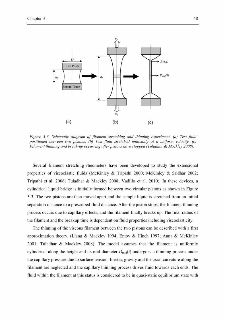
Chapter 3 48
Several filament stretching rheometers have been developed to study the extensional
properties of viscoelastic fluids (McKinley & Tripathi 2000; McKinley & Sridhar 2002;
Tripathi et al. 2006; Tuladhar & Mackley 2008; Vadillo et al. 2010). In these devices, a
cylindrical liquid bridge is initially formed between two circular pistons as shown in Figure
3-3. The two pistons are then moved apart and the sample liquid is stretched from an initial
separation distance to a prescribed fluid distance. After the piston stops, the filament thinning
process occurs due to capillary effects, and the filament finally breaks up. The final radius of
the filament and the breakup time is dependent on fluid properties including viscoelasticity.
The thinning of the viscous filament between the two pistons can be described with a first
approximation theory. (Liang & Mackley 1994; Entov & Hinch 1997; Anna & McKinley
2001; Tuladhar & Mackley 2008). The model assumes that the filament is uniformly
cylindrical along the height and its mid-diameter Dmid(t) undergoes a thinning process under
the capillary pressure due to surface tension. Inertia, gravity and the axial curvature along the
filament are neglected and the capillary thinning process drives fluid towards each ends. The
fluid within the filament at this status is considered to be in quasi-static equilibrium state with
Figure 3-3. Schematic diagram of filament stretching and thinning experiment. (a) Test fluid positioned between two pistons. (b) Test fluid stretched uniaxially at a uniform velocity. (c) Filament thinning and break-up occurring after pistons have stopped (Tuladhar & Mackley 2008).

Chapter 3 49
the combined viscous and viscoelastic forces within the filament, and Dmid(t) evolves with the
following relation:
)(2)(3
tDt
midPS
στεη =∆+ (3-13)
where ηS is the solvent viscosity, �� is the strain rate, σ is the surface tension and Δ�� is the
polymeric tensile stress difference.
An apparent extensional viscosity (ηE) for the axial cylindrical filament can then be
obtained from the mid-filament diameter by taking the ratio of the capillary pressure in the
filament to the instantaneous strain rate in Eq. (3-13) (McKinley & Tripathi 2000; Anna &
McKinley 2001)
dttdDX
ttP
SE /)()12(
)()(3
min−−=
∆+=
σετηη
(3-14)
where X is a coefficient which takes into account the deviation of the shape of the filament
from a uniform cylindrical thread due to inertia and gravity.
3.4 Dimensionless groups relevant to drop generation and impact
Various kinds of free surface deformations are involved in the inkjet printing process of
Newtonian and non-Newtonian fluids. Systematically understanding such flows can be very
difficult owing to the importance of the large number of different forces such as viscosity,
capillarity, and inertia as well as elasticity. A good approach to describe the fluid mechanical
aspects of the jetting and impact process of complex fluids is through the tools of
dimensional analysis (McKinley 2005). This section reviews the various dimensionless
groups that are encountered in the inkjet printing of viscous or viscoelastic fluids.
Liquid drop impact and spreading is normally controlled by inertia, capillary force and
viscous dissipation. These phenomena may be characterised by dimensionless parametric
groups such as the Reynolds number (Re), Weber number (We), Capillary number (Ca) and
Bond number (Bo) which are defined as follows.
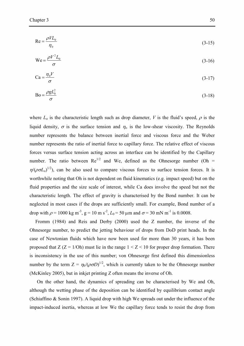
Chapter 3 50
0
0Reη
ρVL= (3-15)
σρ 0
2
We LV= (3-16)
ση V0Ca = (3-17)
σρ 2
0Bo gL= (3-18)
where Lo is the characteristic length such as drop diameter, V is the fluid’s speed, ρ is the
liquid density, σ is the surface tension and ηο is the low-shear viscosity. The Reynolds
number represents the balance between inertial force and viscous force and the Weber
number represents the ratio of inertial force to capillary force. The relative effect of viscous
forces versus surface tension acting across an interface can be identified by the Capillary
number. The ratio between Re1/2 and We, defined as the Ohnesorge number (Oh =
η/(ρσLo)1/2), can be also used to compare viscous forces to surface tension forces. It is
worthwhile noting that Oh is not dependent on fluid kinematics (e.g. impact speed) but on the
fluid properties and the size scale of interest, while Ca does involve the speed but not the
characteristic length. The effect of gravity is characterised by the Bond number. It can be
neglected in most cases if the drops are sufficiently small. For example, Bond number of a
drop with ρ = 1000 kg m-3, g = 10 m s-2, L0 = 50 µm and σ = 30 mN m-1 is 0.0008.
Fromm (1984) and Reis and Derby (2000) used the Z number, the inverse of the
Ohnesorge number, to predict the jetting behaviour of drops from DoD print heads. In the
case of Newtonian fluids which have now been used for more than 30 years, it has been
proposed that Z (Z = 1/Oh) must lie in the range 1 < Z < 10 for proper drop formation. There
is inconsistency in the use of this number; von Ohnesorge first defined this dimensionless
number by the term Z = η0/(ρσD)1/2, which is currently taken to be the Ohnesorge number
(McKinley 2005), but in inkjet printing Z often means the inverse of Oh.
On the other hand, the dynamics of spreading can be characterised by We and Oh,
although the wetting phase of the deposition can be identified by equilibrium contact angle
(Schiaffino & Sonin 1997). A liquid drop with high We spreads out under the influence of the
impact-induced inertia, whereas at low We the capillary force tends to resist the drop from

Chapter 3 51
spreading at the contact line. The relative importance between the capillary and viscous
forces that resist spreading is scaled by the Ohnesorge number. At high Oh fluid’s viscosity
plays a major role in inhibiting drop spreading and at low Oh the dominant role is played by
surface tension. As shown in Figure 3-4, the conditions for CIJ and DoD inkjet printing lie
predominantly in a regime where the drop spreading is dominated by inertial forces and
resisted primarily by viscous forces.
In analogous fashion, free surface flow of non-Newtonian fluids can be characterised by
the Weissenberg number (Wi), Elasticity number (El) and Elasto-capillary number (Ec).
ελ c=Wi (3-19)
20
ReWiEl
Dρλη
== (3-20)
Di
0CaWEc
ηλσ
== (3-21)
The Weissenberg number is defined as the product of the longest or characteristic
relaxation time (λc) of the test fluid and the shear rate or elongational rate (��) of the fluid
Figure 3-4. Schematic diagram adapted from Schiaffino and Sonin (1997) showing four regimes of behaviour for a liquid drop on impact, based on the values of Weber and Ohnesorge numbers (Martin 2008).
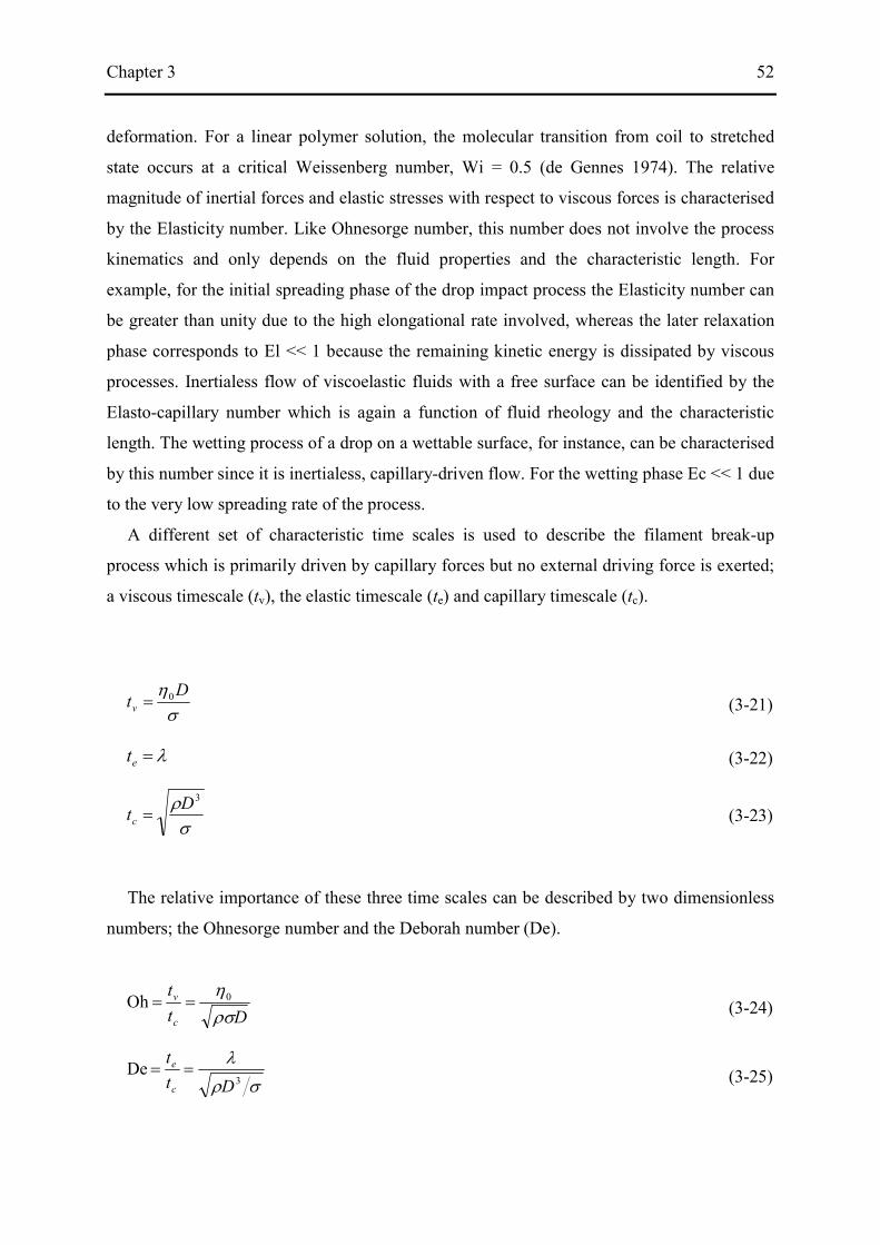
Chapter 3 52
deformation. For a linear polymer solution, the molecular transition from coil to stretched
state occurs at a critical Weissenberg number, Wi = 0.5 (de Gennes 1974). The relative
magnitude of inertial forces and elastic stresses with respect to viscous forces is characterised
by the Elasticity number. Like Ohnesorge number, this number does not involve the process
kinematics and only depends on the fluid properties and the characteristic length. For
example, for the initial spreading phase of the drop impact process the Elasticity number can
be greater than unity due to the high elongational rate involved, whereas the later relaxation
phase corresponds to El << 1 because the remaining kinetic energy is dissipated by viscous
processes. Inertialess flow of viscoelastic fluids with a free surface can be identified by the
Elasto-capillary number which is again a function of fluid rheology and the characteristic
length. The wetting process of a drop on a wettable surface, for instance, can be characterised
by this number since it is inertialess, capillary-driven flow. For the wetting phase Ec << 1 due
to the very low spreading rate of the process.
A different set of characteristic time scales is used to describe the filament break-up
process which is primarily driven by capillary forces but no external driving force is exerted;
a viscous timescale (tv), the elastic timescale (te) and capillary timescale (tc).
ση Dtv
0=
(3-21)
λ=et
(3-22)
σρ 3Dtc =
(3-23)
The relative importance of these three time scales can be described by two dimensionless
numbers; the Ohnesorge number and the Deborah number (De).
Dtt
c
v
ρση0Oh == (3-24)
σρ
λ3
DeDt
t
c
e == (3-25)

Chapter 3 53
As mentioned above, the Ohnesorge number represents the ratio between viscous time
scale and capillary time scale. The Deborah number for free surface viscoelastic flows
represents the balance between the time scale for elastic stress relaxation and the capillary
break-up time of an inviscid jet. These two parameters are determined only by the fluid’s own
parameters and the geometry of interest, not by a kinematic term, nor by shear rate/
elongational rate like the Weissenberg number. An operating space for instruments such as a
filament stretching rheometer and other self-thinning free surface processes involving non-
Newtonian fluids can be identified by these two parameters as illustrated in Figure 3-5
(McKinley 2005).
Figure 3-5. An operating diagram for capillary self-thinning and break-up of non-Newtonian fluids (McKinley 2005).
Chapter 4 54
4. Materials and experimental methods
4.1 Introduction
Chapter 4 describes the materials, fluid characterisation methods and high-speed imaging
systems that were used in this work. Fundamental properties and conditions of model fluids
and substrates for the experiments are presented in section 4.2. Section 4.3 provides a
detailed procedure for various fluid characterisation techniques with some typical examples
of results. The experimental method used to study for the collision of two liquid jets is
described in section 4.4, which is then used in chapters 5 and 6 to evaluate ink as a
characterisation method to assess the printability of non-Newtonian inkjet fluids. Finally,
section 4.5 describes the drop deposition and impact system together with the image
processing technique used in this work. Research questions 1 and 3 are addressed in this
chapter.
4.2 Fluids and substrates
4.2.1 Fluids
Two different model fluid systems, which have similar fluid properties to commercial inks
used for printed electronics, were used to systematically study the influence of fluid
properties such as viscosity, surface tension and elasticity including polymer concentration
and molecular weight: solutions of polystyrene (PS) in diethylphthalate (DEP), and
polyethylene oxide (PEO) in a glycerol/water (GW) mixture.
Monodisperse PS, having a poly-dispersity index or PDI < 1.1 of three different molecular
weights of 1.10 105, 2.10 105, and 4.88 105 g mol-1 (Dow Chemicals, USA) was
dissolved in DEP (σ = 1.12 g/mL, 99.5% purity, Sigma-Aldrich, UK) to give various
concentrations from 0.01 wt% to 1 wt%. DEP is a relatively good solvent for PS at room
temperature. These three groups of solutions are designated PS 110K, PS 210K and PS 488K,
respectively. The low-shear rate viscosities were measured with a Viscolite 700 vibrational

Chapter 4 55
viscometer (Hydramotion Ltd., UK), and were all between 10 and 13 mPa s at 22°C. The
equilibrium surface tension (~ 37 mN m-1) was measured with a bubble tensiometer (SITA
proline 15) and was almost the same for all polymer concentrations at this temperature. The
values of low-shear viscosity and surface tension are effectively similar to those of
commercial inks.
Polydisperse PEO (Sigma-Aldrich, UK) was dissolved in mixtures of glycerol (Sigma-
Aldrich, UK) and pure water (60%:40% by weight) to give concentrations from 0.00001 wt%
to 1 wt%. PEO was used with seven different average molecular weights (all in g mol-1): 1.0
105 (solution designated PEO 100K); 2.0 105 (PEO 200K); 3.0 105 (PEO 300K); 6.0
105 (PEO 600K); 1.0 106 (PEO 1M); 2.0 106 (PEO 2M); and 5.0 106 (PEO 5M).
The viscosities of these solutions lay between 10 and 13 mPa s and the equilibrium surface
tension was almost constant at ~ 56 mN m-1 for all PEO concentrations. The poly-dispersity
index for the PEO samples was unknown but a recent study of the dispersion procedure of
high molecular weight PEO in aqueous solution quotes a PDI = 3.33 (Bossard et al. 2009),
while Tirtaatmadja et al. (2006) quote PDI ~ 1.8 for PEO 1M as a typical value, but effective
PDI may be affected by stresses in PEO preparation (Bossard et al. 2009) or even during
jetting (Xu et al. 2007; A-Alamry et al. 2010).
Newtonian mixtures of glycerol–water (GW) were also used to investigate the influence of
viscosity and surface tension. The viscosity of GW 50-50 (50:50% by weight) was 6 mPa s,
almost a half GW 60-40 (η = 10 mPa s) but equilibrium surface tension was nearly the same
(~57 mN m-1).
All the solutions except some solutions of PEO 100K had polymer concentrations below
the critical concentration (c*) defined as the concentration where the polymer chains start to
interact with each other (Graessley 1980), and thus were in the dilute regime. According to
the Zimm theory, the intrinsic viscosity of diluted polymer solutions with hydrodynamic
interaction and solvent-polymer interactions is proportional to MW(3ν-1) for long chains, where
ν is the solvent quality exponent and MW is the molecular weight. Intrinsic viscosity ([η])
values for the PS and PEO solutions were estimated from the respective composite Mark–
Houwink–Sakurada equations as follows (Clasen et al. 2006; Tirtaatmadja et al. 2006):
[η]PS = 0.0081Mw0.704 [cm3g-1] for PS solutions in DEP (4-1)
[η]PEO = 0.0072Mw0.65 [cm3g-1] for PEO solutions in GW (4-2)
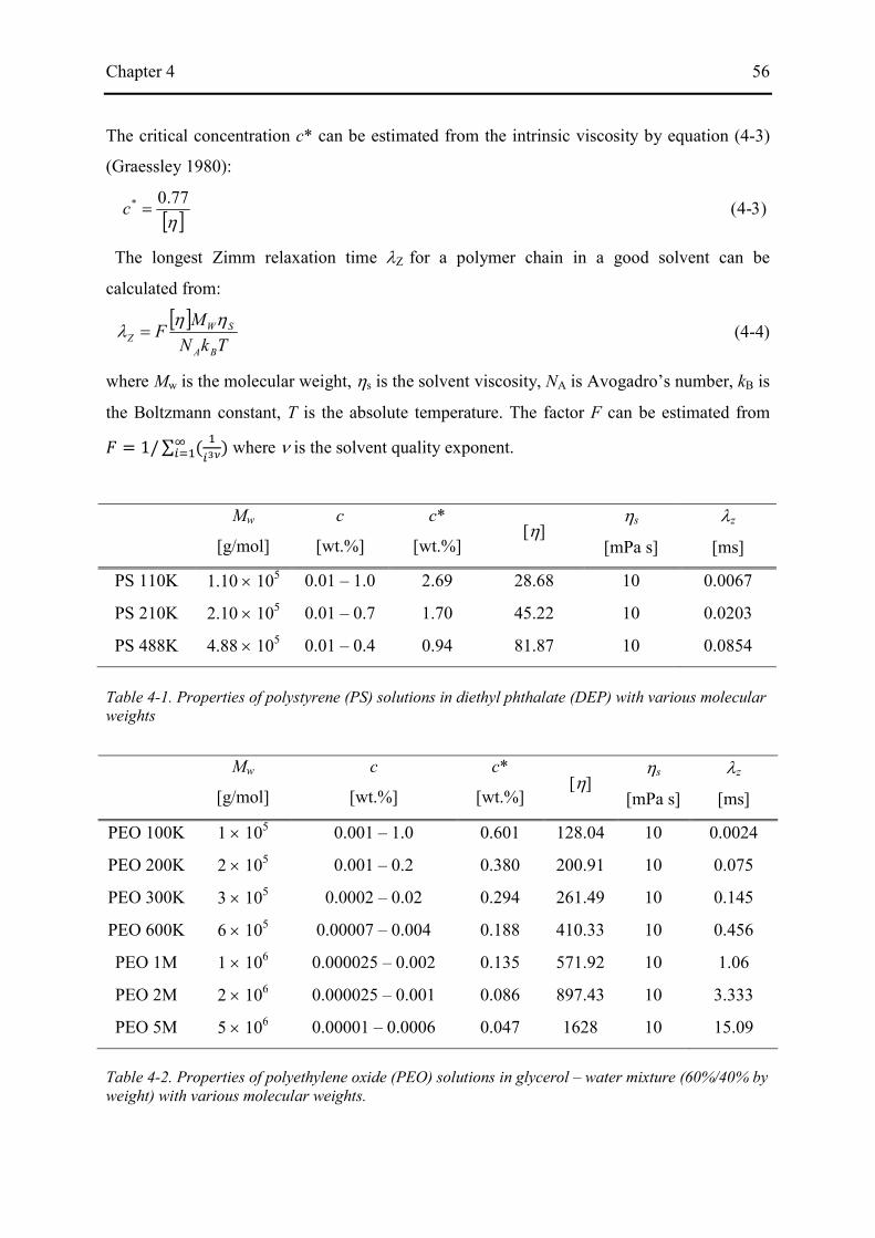
Chapter 4 56
The critical concentration c* can be estimated from the intrinsic viscosity by equation (4-3)
(Graessley 1980):
[ ]η77.0* =c (4-3)
The longest Zimm relaxation time λΖ for a polymer chain in a good solvent can be
calculated from:
[ ]TkN
MFBA
SWZ
ηηλ = (4-4)
where Mw is the molecular weight, ηs is the solvent viscosity, NA is Avogadro’s number, kB is
the Boltzmann constant, T is the absolute temperature. The factor F can be estimated from
� = 1/ ∑ ( ����)�
��� where ν is the solvent quality exponent.
Mw
[g/mol]
c
[wt.%]
c*
[wt.%] [η]
ηs
[mPa s]
λz
[ms]
PS 110K 1.10 × 10⁵ 0.01 – 1.0 2.69 28.68 10 0.0067
PS 210K 2.10 × 10⁵ 0.01 – 0.7 1.70 45.22 10 0.0203
PS 488K 4.88 × 10⁵ 0.01 – 0.4 0.94 81.87 10 0.0854
Table 4-1. Properties of polystyrene (PS) solutions in diethyl phthalate (DEP) with various molecular weights
Mw
[g/mol]
c
[wt.%]
c*
[wt.%] [η]
ηs
[mPa s]
λz
[ms]
PEO 100K 1 × 10⁵ 0.001 – 1.0 0.601 128.04 10 0.0024
PEO 200K 2 × 10⁵ 0.001 – 0.2 0.380 200.91 10 0.075
PEO 300K 3 × 10⁵ 0.0002 – 0.02 0.294 261.49 10 0.145
PEO 600K 6 × 10⁵ 0.00007 – 0.004 0.188 410.33 10 0.456
PEO 1M 1 × 10⁶ 0.000025 – 0.002 0.135 571.92 10 1.06
PEO 2M 2 × 10⁶ 0.000025 – 0.001 0.086 897.43 10 3.333
PEO 5M 5 × 10⁶ 0.00001 – 0.0006 0.047 1628 10 15.09
Table 4-2. Properties of polyethylene oxide (PEO) solutions in glycerol – water mixture (60%/40% by weight) with various molecular weights.
Chapter 4 57
Tables 4-1 and 4-2 list the measured properties of the PS and PEO solutions used, together
with the value of c* and λZ estimated from equations (4-3) and (4-4).
4.1.2 Substrates
Indium tin oxide (ITO)-coated glass slides (50 × 50 mm), which are commonly used as a
base substrate for OLED display, were used as model wettable substrates and polytetra-
fluoroethylene (PTFE)-coated glass slides (50 × 50 mm) as non-wettable substrates. These
were supplied by CDT Ltd, Cambridgeshire, UK. The substrates were carefully cleaned with
distilled water, acetone and isopropanol in sequence. In order to produce highly wettable
surface, the ITO-coated glass substrates were also modified with a bench-top corona treater
(Labtec) purchased from Tantech, Denmark to increase their surface energy. The corona
discharge was produced between an electrode connected to a high-voltage generator and
ground with a gap of 1.4 mm. The air ionised by the discharge is believed to oxidise the
surface of the substrate, increasing its surface energy and thus reducing the contact angle
between the printed drop and the substrate. The high-voltage generator was set to 21 kV and
the electrode was moved above the surface at the speed of ∼20 mm s-1. Each substrate was
treated five times consecutively in this way before use.
The equilibrium contact angle θeq
for DEP on the as-received ITO/glass substrate was
measured with mm-sized water drops in a sessile drop experiment to be 32 ± 2°, and after
corona treatment was reduced to 4 ± 2°. The PTFE-coated glass shows hydrophobic
characteristic with θeq of 78 ± 2°. For these measurements ~2mm-sized drops were ejected
from a syringe with internal diameter of 0.15 mm and their images were captured with a
digital camera (DCM 300, Hangzhou Huaxin IC Technology, China)and a blue LED.
4.3 Rheological measurements
4.3.1 Apparent viscosity
Ink jet fluids are usually characterised by their low shear rate viscosity and sometimes the
apparent viscosity as a function of shear rate is also used to detect any shear thinning
behaviour (Hoath et al. 2009). A Vibrational viscometer (Viscolite 700, Hydramotion Ltd.,
York, UK) was used to measure low shear rate viscosity. The solid stainless steel sensor
element
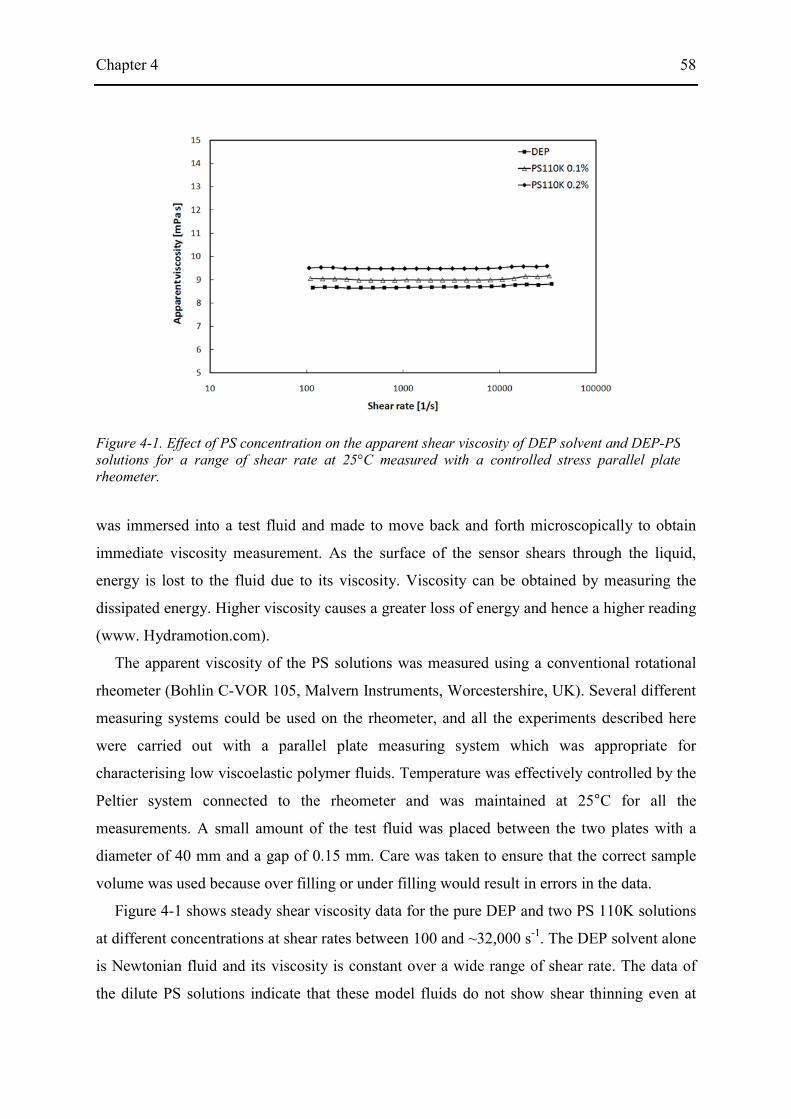
Chapter 4 58
was immersed into a test fluid and made to move back and forth microscopically to obtain
immediate viscosity measurement. As the surface of the sensor shears through the liquid,
energy is lost to the fluid due to its viscosity. Viscosity can be obtained by measuring the
dissipated energy. Higher viscosity causes a greater loss of energy and hence a higher reading
(www. Hydramotion.com).
The apparent viscosity of the PS solutions was measured using a conventional rotational
rheometer (Bohlin C-VOR 105, Malvern Instruments, Worcestershire, UK). Several different
measuring systems could be used on the rheometer, and all the experiments described here
were carried out with a parallel plate measuring system which was appropriate for
characterising low viscoelastic polymer fluids. Temperature was effectively controlled by the
Peltier system connected to the rheometer and was maintained at 25°C for all the
measurements. A small amount of the test fluid was placed between the two plates with a
diameter of 40 mm and a gap of 0.15 mm. Care was taken to ensure that the correct sample
volume was used because over filling or under filling would result in errors in the data.
Figure 4-1 shows steady shear viscosity data for the pure DEP and two PS 110K solutions
at different concentrations at shear rates between 100 and ~32,000 s-1. The DEP solvent alone
is Newtonian fluid and its viscosity is constant over a wide range of shear rate. The data of
the dilute PS solutions indicate that these model fluids do not show shear thinning even at
Figure 4-1. Effect of PS concentration on the apparent shear viscosity of DEP solvent and DEP-PS solutions for a range of shear rate at 25°C measured with a controlled stress parallel plate rheometer.
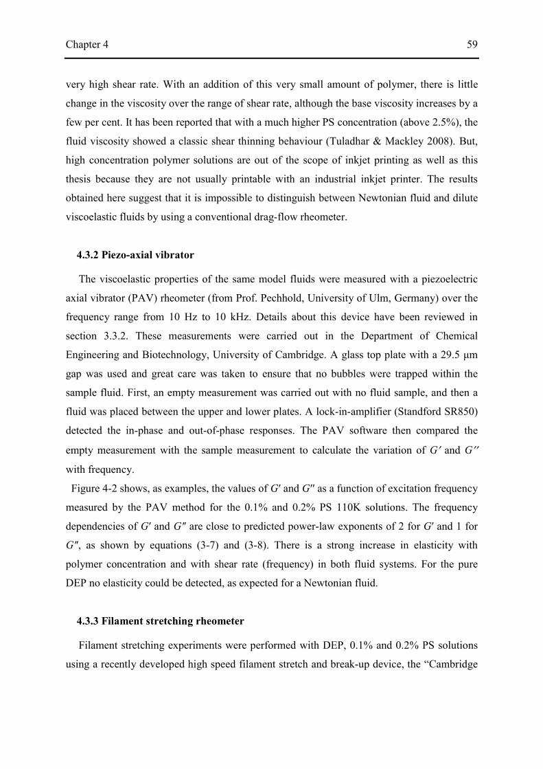
Chapter 4 59
very high shear rate. With an addition of this very small amount of polymer, there is little
change in the viscosity over the range of shear rate, although the base viscosity increases by a
few per cent. It has been reported that with a much higher PS concentration (above 2.5%), the
fluid viscosity showed a classic shear thinning behaviour (Tuladhar & Mackley 2008). But,
high concentration polymer solutions are out of the scope of inkjet printing as well as this
thesis because they are not usually printable with an industrial inkjet printer. The results
obtained here suggest that it is impossible to distinguish between Newtonian fluid and dilute
viscoelastic fluids by using a conventional drag-flow rheometer.
4.3.2 Piezo-axial vibrator
The viscoelastic properties of the same model fluids were measured with a piezoelectric
axial vibrator (PAV) rheometer (from Prof. Pechhold, University of Ulm, Germany) over the
frequency range from 10 Hz to 10 kHz. Details about this device have been reviewed in
section 3.3.2. These measurements were carried out in the Department of Chemical
Engineering and Biotechnology, University of Cambridge. A glass top plate with a 29.5 μm
gap was used and great care was taken to ensure that no bubbles were trapped within the
sample fluid. First, an empty measurement was carried out with no fluid sample, and then a
fluid was placed between the upper and lower plates. A lock-in-amplifier (Standford SR850)
detected the in-phase and out-of-phase responses. The PAV software then compared the
empty measurement with the sample measurement to calculate the variation of G′ and G′′
with frequency.
Figure 4-2 shows, as examples, the values of G′ and G′′ as a function of excitation frequency
measured by the PAV method for the 0.1% and 0.2% PS 110K solutions. The frequency
dependencies of G′ and G'′ are close to predicted power-law exponents of 2 for G′ and 1 for
G'′, as shown by equations (3-7) and (3-8). There is a strong increase in elasticity with
polymer concentration and with shear rate (frequency) in both fluid systems. For the pure
DEP no elasticity could be detected, as expected for a Newtonian fluid.
4.3.3 Filament stretching rheometer
Filament stretching experiments were performed with DEP, 0.1% and 0.2% PS solutions
using a recently developed high speed filament stretch and break-up device, the “Cambridge
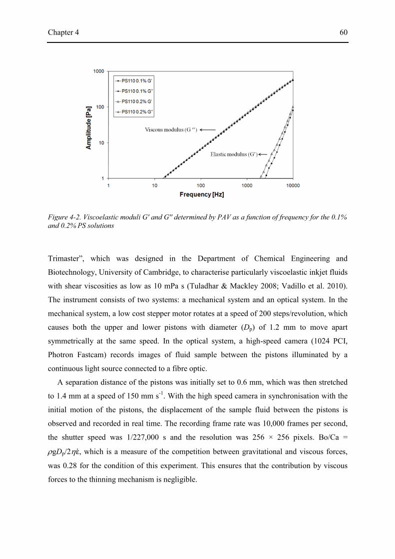
Chapter 4 60
Trimaster”, which was designed in the Department of Chemical Engineering and
Biotechnology, University of Cambridge, to characterise particularly viscoelastic inkjet fluids
with shear viscosities as low as 10 mPa s (Tuladhar & Mackley 2008; Vadillo et al. 2010).
The instrument consists of two systems: a mechanical system and an optical system. In the
mechanical system, a low cost stepper motor rotates at a speed of 200 steps/revolution, which
causes both the upper and lower pistons with diameter (Dp) of 1.2 mm to move apart
symmetrically at the same speed. In the optical system, a high-speed camera (1024 PCI,
Photron Fastcam) records images of fluid sample between the pistons illuminated by a
continuous light source connected to a fibre optic.
A separation distance of the pistons was initially set to 0.6 mm, which was then stretched
to 1.4 mm at a speed of 150 mm s-1. With the high speed camera in synchronisation with the
initial motion of the pistons, the displacement of the sample fluid between the pistons is
observed and recorded in real time. The recording frame rate was 10,000 frames per second,
the shutter speed was 1/227,000 s and the resolution was 256 × 256 pixels. Bo/Ca =
ρgDp/2ηε� , which is a measure of the competition between gravitational and viscous forces,
was 0.28 for the condition of this experiment. This ensures that the contribution by viscous
forces to the thinning mechanism is negligible.
Figure 4-2. Viscoelastic moduli G' and G'' determined by PAV as a function of frequency for the 0.1% and 0.2% PS solutions
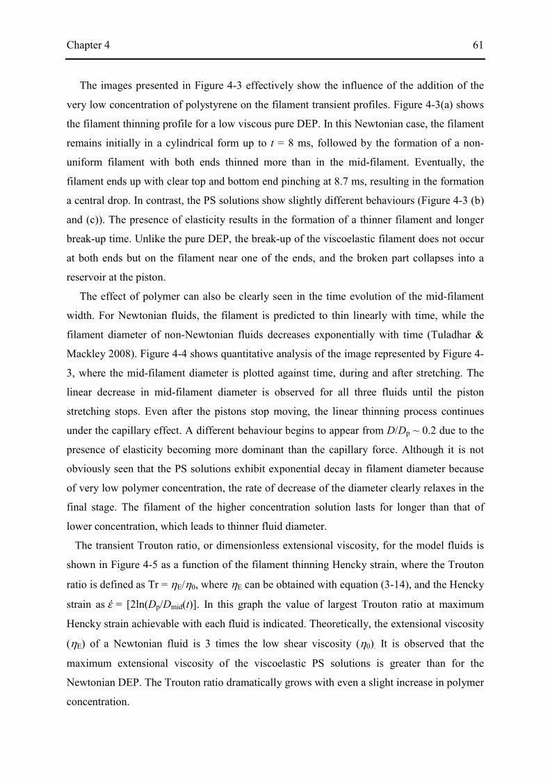
Chapter 4 61
The images presented in Figure 4-3 effectively show the influence of the addition of the
very low concentration of polystyrene on the filament transient profiles. Figure 4-3(a) shows
the filament thinning profile for a low viscous pure DEP. In this Newtonian case, the filament
remains initially in a cylindrical form up to t = 8 ms, followed by the formation of a non-
uniform filament with both ends thinned more than in the mid-filament. Eventually, the
filament ends up with clear top and bottom end pinching at 8.7 ms, resulting in the formation
a central drop. In contrast, the PS solutions show slightly different behaviours (Figure 4-3 (b)
and (c)). The presence of elasticity results in the formation of a thinner filament and longer
break-up time. Unlike the pure DEP, the break-up of the viscoelastic filament does not occur
at both ends but on the filament near one of the ends, and the broken part collapses into a
reservoir at the piston.
The effect of polymer can also be clearly seen in the time evolution of the mid-filament
width. For Newtonian fluids, the filament is predicted to thin linearly with time, while the
filament diameter of non-Newtonian fluids decreases exponentially with time (Tuladhar &
Mackley 2008). Figure 4-4 shows quantitative analysis of the image represented by Figure 4-
3, where the mid-filament diameter is plotted against time, during and after stretching. The
linear decrease in mid-filament diameter is observed for all three fluids until the piston
stretching stops. Even after the pistons stop moving, the linear thinning process continues
under the capillary effect. A different behaviour begins to appear from D/Dp ~ 0.2 due to the
presence of elasticity becoming more dominant than the capillary force. Although it is not
obviously seen that the PS solutions exhibit exponential decay in filament diameter because
of very low polymer concentration, the rate of decrease of the diameter clearly relaxes in the
final stage. The filament of the higher concentration solution lasts for longer than that of
lower concentration, which leads to thinner fluid diameter.
The transient Trouton ratio, or dimensionless extensional viscosity, for the model fluids is
shown in Figure 4-5 as a function of the filament thinning Hencky strain, where the Trouton
ratio is defined as Tr = ηE/η0, where ηE can be obtained with equation (3-14), and the Hencky
strain as �� = [2ln(Dp/Dmid(t)]. In this graph the value of largest Trouton ratio at maximum
Hencky strain achievable with each fluid is indicated. Theoretically, the extensional viscosity
(ηE) of a Newtonian fluid is 3 times the low shear viscosity (η0). It is observed that the
maximum extensional viscosity of the viscoelastic PS solutions is greater than for the
Newtonian DEP. The Trouton ratio dramatically grows with even a slight increase in polymer
concentration.

Chapter 4 62
Figure 4-3. Sequential images of the filament break-up captured with the Trimaster in the extensional viscometer mode for (a) pure DEP, (b) 0.1% PS110K in DEP and (c) 0.2% PS110K in DEP
Figure 4-4. Evolution of mid-filament diameter in time for DEP, 0.1% and 0.2% PS solutions. (−)piston cessation of motion.

Chapter 4 63
4.4 Experimental arrangement for collision of two liquid jets
The oblique collision of two cylindrical laminar jets leads to the liquid flowing radially
outwards from the impact point, creating a thin oval sheet bounded by a thicker rim, as shown
in Figure 4-6. This sheet lies in a plane perpendicular to the plane containing the two jets and
disintegrates into ligaments or droplets as the flow rate is increased. The break-up of the edge
(rim) of the sheet becomes remarkably regular within a certain range of Reynolds and Weber
numbers of the jets. It was discovered through this work that this atomisation pattern
produced by the oblique collision of two impinging jets might be used to assess the
rheological properties of polymer-based inks. Chapter 5 and 6 will discuss how this method
can be used to predict the printability of a test ink without involving an expensive print head.
A schematic diagram of the apparatus is presented in Figure 4-7. Fluid from a reservoir
was pumped through flexible tubing with an inner diameter of 6 mm via a flowmeter
(FHKSC, Digmesa AG, Switzerland) into a flow splitter, and divided between two identical
stainless steel hypodermic needles (with square ends) having an internal diameter Dj of 0.85
mm and length of 25.4 mm. The detailed arrangement of the nozzles and jets is shown in
Figure 4-6. The jets were laminar and identical in flux (as measured by collecting fluid from
each needle for a fixed time period) within an accuracy of 1 %. The jet lengths Lj1 and Lj2,
Figure 4-5. Transient Trouton ratio of DEP, 0.1% and 0.2% PS solutions at their maximum Hencky strain just before break-up
Chapter 4 64
defined as the distance from the ends of the nozzles to the point of impact, were varied
between 3.5 and 18 mm; in most experiments the two lengths were different. The angle 2α
between the axes of the two jets was held constant at 78° in all the experiments. This angle
was found in preliminary experiments to provide well-developed fishbone patterns. Glycerol-
water mixtures were used as test fluids with various glycerol concentrations. The viscosities
of these Newtonian solutions lay between 4 and 30 mPa s. Equilibrium surface tension for
Figure 4-6. Liquid sheet produced by oblique collision of two jets with diameter Dj, velocity Vj, lengths Lj1 and Lj2 and included angle 2α
Figure 4-7. Schematic diagram of the experimental apparatus. Internal diameter of nozzles: 0.85 mm, flash duration: ~1 µs.

Chapter 4 65
each test fluid was effectively constant at 58 ± 1 mN m-1 for all the concentrations. The rotor-
based flow-meter with an electrical pulse output was calibrated for each fluid mixture by
measuring the frequency of the pulses and the volume ejected from the needles over a set
time. The jet velocity (Vj) was varied by changing the speed of the pump, from ~1 to 6 m s-1.
The corresponding Reynolds and Weber numbers for glycerol-water mixtures, defined in
terms of the jet diameter, were in the range 70 < Re < 700 and 30 < We < 600.
Single-flash photography with back-illumination was used to capture individual images of
the jet interaction region and to extract quantitative information such as the sizes of the
resulting droplets, their spacing and the angle between the droplet streams. The light source
was a xenon lamp with ~1 µs flash duration which was sufficiently short to avoid motion blur,
and the image was captured with a 10 mega pixel digital single lens reflex camera (Nikon
D40X) kitted with a NIKKOR 55-200 mm lens . The axis of the optical system was normal to
the fluid sheet. In this experimental set-up the flash, camera and flowmeter were controlled
and synchronised by a PC data acquisition board (NI-6016, National Instruments, Berkshire,
UK) programmed with Labview. A digital pulse signal is sent from the NI-6016 to the remote
controller of the camera, which generates specific radio frequency signals to the camera to
operate with a 1/3 s shutter speed. Another pulse was produced with a specified delay time
from the first one and transferred to the flash controller, to synchronise the flash with the
shutter opening. At the same time a series of digital signals was acquired from the flowmeter,
so that for each recorded image the flow rate and hence jet velocity could be accurately
determined with a measurement error of 0.2%.
Image processing was performed in several steps using National Instruments Vision
Assistant as shown in Figure 4-8. An 8 bit grayscale image (b) was obtained by extracting the
intensity plane from an original HSI (Hue, Saturation and Intensity) image (a). In the next
step, a simple thresholding technique was applied to isolate objects of interest from the
background in the image. In this technique, all the pixels that belong to a gray-level interval
was set to 1 and all the other pixels in the image were set to 0. Through this process, the
greyscale image with pixel values ranging from 0 to 255 was converted into a binary image
with pixel values of 0 or 1 (c). Binary morphological operations were also performed in order
to remove unwanted information, thus improving the information in the binary image. Finally,
particle analysis was carried out to detect connected regions or groupings of pixels in the
image and then measurements of those regions were made to obtain information such as drop
diameter, drop spacing and ligament length (d).
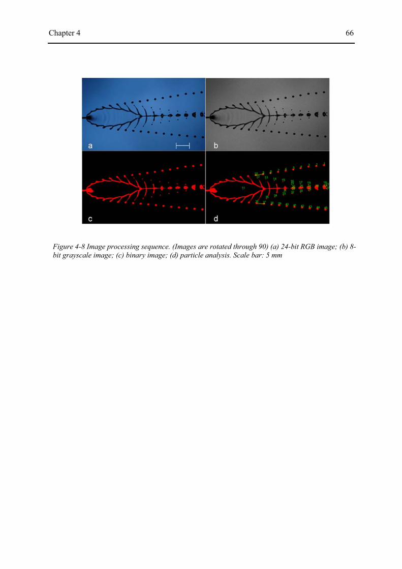
Chapter 4 66
Figure 4-8 Image processing sequence. (Images are rotated through 90) (a) 24-bit RGB image; (b) 8-bit grayscale image; (c) binary image; (d) particle analysis. Scale bar: 5 mm
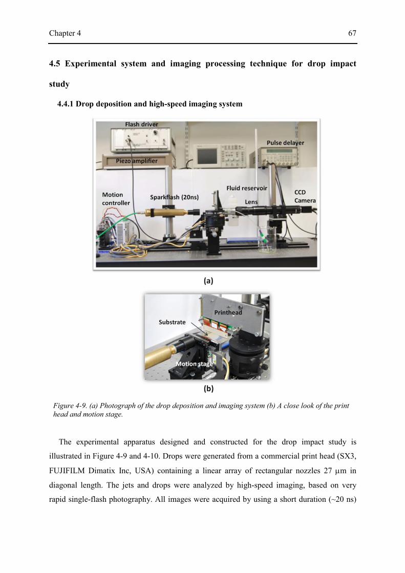
Chapter 4 67
4.5 Experimental system and imaging processing technique for drop impact
study
4.4.1 Drop deposition and high-speed imaging system
The experimental apparatus designed and constructed for the drop impact study is
illustrated in Figure 4-9 and 4-10. Drops were generated from a commercial print head (SX3,
FUJIFILM Dimatix Inc, USA) containing a linear array of rectangular nozzles 27 µm in
diagonal length. The jets and drops were analyzed by high-speed imaging, based on very
rapid single-flash photography. All images were acquired by using a short duration (~20 ns)
Figure 4-9. (a) Photograph of the drop deposition and imaging system (b) A close look of the print head and motion stage.

Chapter 4 68
flash light (Nanolite, High-Speed Photo-Systeme, Germany) and a high resolution CCD
camera (sensor 1290 × 960 pixels: GC 1290, Prosilica, Germany). The high magnification
optical system consisted of a long working distance 20× objective lens (M Plan Apo,
Mitutoyo, UK) and a 12× zoom lens (Zoom 6000, Navitar, USA) and was capable of imaging
a sub-30 µm drop with high resolution. The pixel size in the image was 0.135 µm.
The substrate was supported on a miniature linear motor stage (MX80L, Parker
Automation, UK) with a resolution of 1 µm and a travel range of 50 mm. The standoff
distance of the print head from the print head to the substrate was 0.6 mm, by which distance
the ejected fluid ligament had collapsed to form a single drop. All the components were
Figure 4-10. (a) Signal flow of the inkjet deposition apparatus (b) typical drive wave form for drop ejection
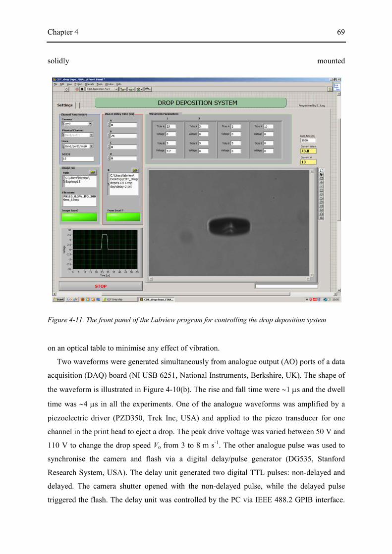
Chapter 4 69
solidly mounted
on an optical table to minimise any effect of vibration.
Two waveforms were generated simultaneously from analogue output (AO) ports of a data
acquisition (DAQ) board (NI USB 6251, National Instruments, Berkshire, UK). The shape of
the waveform is illustrated in Figure 4-10(b). The rise and fall time were ∼1 µs and the dwell
time was ∼4 µs in all the experiments. One of the analogue waveforms was amplified by a
piezoelectric driver (PZD350, Trek Inc, USA) and applied to the piezo transducer for one
channel in the print head to eject a drop. The peak drive voltage was varied between 50 V and
110 V to change the drop speed Vo from 3 to 8 m s-1. The other analogue pulse was used to
synchronise the camera and flash via a digital delay/pulse generator (DG535, Stanford
Research System, USA). The delay unit generated two digital TTL pulses: non-delayed and
delayed. The camera shutter opened with the non-delayed pulse, while the delayed pulse
triggered the flash. The delay unit was controlled by the PC via IEEE 488.2 GPIB interface.
Figure 4-11. The front panel of the Labview program for controlling the drop deposition system

Chapter 4 70
After each drop impact event, a trigger signal was sent from the digital output (DO) of the
DAQ to the motion stage to move the substrate through a distance of 100 to 300 µm so that
the next impact event occurred on a fresh area of the substrate. A Labview program was
written to repeat the jetting–deposition–imaging–movement sequence at intervals of 0.2 s
with increasing flash delay times in order to capture a series of images automatically. The
front panel of the program is presented in Figure 4-11 and the brief manual of the programme
can be found in Appendix.
4.4.2 Imaging processing technique
Figure 4-12 (a) and (b) show typical images of the jetting of DEP. For a drop speed of 6
m s-1, the jet appeared at 3 µs after the trigger pulse and detached from the nozzle plate at ~28
µs, with a maximum ligament length of ~170 µm. The ligament retracted and collapsed into
the main drop within ∼50 µs. No satellite drops were formed under these jetting conditions.
Images of drops just before and after impact are seen in Figure 4-12 (c) and (d), which show
both the image of the drop and its reflection in the substrate. The very short duration of the
spark flash avoided significant motion blurring despite the very high magnification. The
National Instrument Vision Development Module was used to enhance images, identify
Figure 4-12. Typical images showing jetting (a and b) and deposition (c and d) of DEP ejected from the Spectra print head. (a) and (b) were taken with 10× objective lens and images (c) and (d) with 20× objective lens. (c) and (d) show the direct images of the drop in the upper half of the frame, together with its reflection in the horizontal surface of the substrate of the substrate in the lower half. Djet = 26.2µm and D0 = 28µm.

Chapter 4 71
objects, and extract quantitative information. The optical system and imaging processing
technique can distinguish the fluid-air interface with a resolution of better than ~ 0.5 µm
(corresponding to maximum 4 pixels). Since the events were highly reproducible, the time
evolution of the event could be investigated by acquiring a series of images with different
delay times. Typical variation in drop position along the direction of flight for DEP was < 1
µm which is equivalent to < 0.2 µs in time variation for a drop speed of 6 m s-1. This
uncertainty in time was important for analysis of the time evolution of drop diameter in the
early stages. The size of a final drop is consistent with errors of 1.5%.
Thresholding was utilised for the images of the fluid patterns produced by the collision of
two liquid jets. In this technique, a single critical grayscale value was applied to all the
images to segment an 8-bit image into two regions: a particle region and a background region.
It was a simple and useful approach to extract relevant information with a high accuracy from
the images captured from the impinging jet experiment in which the objects in the images
were relatively large and the background level was uniform.
Figure 4-13. Edge detection by a simple thresholding technique. A gray level value of 78 was applied to both images (a) and (b) with different background level. Results from the image processing: (c) 110 pixels;(d) 86 pixels in diameter

Chapter 4 72
However, this image processing method could not be applied for the drop impact
experiment using the spark flash due to variation in lighting condition between images. The
intensity of light emitted by the spark flash varied between flashes, and the image histogram
that describes the distribution of the pixel intensity in the images was seriously affected by
the variation. In addition, there was no very distinct demarcation between the object and the
background. Figure 4-13 shows how changing the light intensity of the spark flash causes
errors during the image processing for information extraction. Captured at the same jetting
condition but at different times, two images of identical DEP drops with very different
background grayscale level were selected to examine the effect. In Figure 4-13, image (a) has
a dark background, whereas image (b) is generally much lighter. The same gray level value
of 78 was applied to both images, which resulted in considerable variation in the estimated
drop diameter. As shown in Figure 4-13 (c) and (d), the darker illumination causes the
software to recognise the larger area as an object (110 pixels in diameter), while the brighter
overall intensity reduces the size of the processed drop area (86 pixels in diameter)
It was therefore necessary to develop a light intensity-tolerant edge detection technique to
process the spark-flash illuminated drop images. To do this, an advanced edge detection
(AED) method, which is often used in machine vision applications, was introduced to analyse
Figure 4-14. A commonly used edge characterisation model. (a) grayscale profile; (b) edge length; (c) edge strength; (d) edge location (NI Vision for LabVIEW User Manual)

Chapter 4 73
drop impact images (NI Vision for LabVIEW User Manual). Figure 4-14 shows a commonly
used model for edge characterisation. Gray level intensity was obtained along the line ROI
(Region Of Interest) in the graph. In this model, an edge is defined as a significant change in
the grayscale values between adjacent pixels in an image; edge length is the maximum
distance in which the desired grayscale difference between the edge and the background
ought to occur; edge strength is the minimum difference in the grayscale values between the
background and the edge; edge position is the x, y location of an edge in the test image.
In the AED method, the one-dimensional grayscale profile is first obtained by scanning
pixel by pixel. Next, the edge strength is computed at a given along the pixel profile by
averaging pixels before and after the analysed point. Finally, the difference between these
averages (gradient information) is calculated to determine the contrast. The first and the last
peak of the difference are normally recognised as an edge each side. The two images of
Figure 4-13 were processed to verify this technique. The results for line profile and gradient
information are presented in Figure 4-15. The computed diameters of the drops in Figure 4-
13(a) and (b), the distance between the edges, are 97 and 98 pixels respectively, which proves
that this technique is not significantly affected by lighting conditions.
Figure 4-15. (a, b) Line profile and (c, d) gradient information for drop images with different background in Figure 4-13 (a, b) respectively
Chapter 5 74
5. Collision of two liquid jets: I. Newtonian fluid
5.1 Introduction
Oblique collision of two liquid jets results in various regimes of behaviour which depend
on the jet velocities and the liquid properties. Within a certain range of Reynolds and Weber
numbers, the impinging jets form a liquid sheet which then breaks up into a regular
succession of ligaments and droplets, a so-called ‘fishbone’ pattern. Over this and the next
chapter, we explore a possibility that this atomisation phenomenon could provide information
about the printability of a viscoelastic fluid in inkjet printing, without using a real printhead.
This chapter reports a detailed investigation of the formation, destabilisation and
fragmentation of the liquid sheet formed by the oblique impact of jets of Newtonian liquids at
low Re and We. Then, in the next chapter we discuss how the periodic atomisation pattern
can be used to assess the jetting performance of a polymer ink.
As described in chapter 4, we use single-flash photography to observe the various regimes
of behaviour produced by the oblique impact of Newtonian liquids. Glycerol-water mixtures
are used as test fluids with various glycerol concentrations such that its viscosity is varied
between 4 mPa s and 30 mPa s. Experimental observations of the various fluid patterns from
the collision are provided in sections 5.2.1 to 5.2.3 with the results on effect of difference in
jet length, jet alignment and fluid viscosity on the resulting patterns. The size of the fluid
sheet as well as the drop size and the thickness of the rim of the sheet are shown in section
5.2.4, followed by introducing various methods to induce the fishbone instabilities by
external perturbation in section 5.2.5. We discuss over sections 5.3.1 to 5.3.4 why some
asymmetry is essential for this type of atomisation pattern to be developed and what causes
the fishbone instability.

Chapter 5 75
5.2 Results
5.2.1 Effects of asymmetry in the collision of two identical jets
Figure 5-1 shows the progression of flow structures formed by the collision of jets with
viscosity 10 mPa s, for jet lengths Lj1 and Lj2 of 3.5 mm and 6.5 mm respectively, as the jet
velocity is increased. Collision at the lowest flow velocity produces oscillating streams (a),
followed at higher velocity by the formation of a chain of fluid sheets in which the elements
are orthogonally linked to each other (b). The initially narrow oval sheet surrounding the jet
impact region becomes wider with increasing flow rate. As the flow rate is increased, small
perturbations on the rim of the sheet trigger fragmentation of the rim leading to periodic
atomization with the formation of ligaments and droplets (the first fishbone regime - c). The
ligaments elongate to a degree that depends on the liquid properties, the asymmetry in the
lengths (Lj1 and Lj2) of the two jets or their alignment, which we discuss below. After the
ligaments become extended to their maximum length, the pattern suddenly converts into a
smooth fluid sheet and chain (d), in which the sheet is much larger than that formed at the
lowest speeds, presumably because of the equilibrium between the surface tension and fluid
inertia on the sheet rim. As the flow rate is further increased, periodic atomization then
occurs with a larger pattern than the first one (second fishbone regime - e). At even higher
flow rates, the sheet enters a regime of violent flapping (f), which was also observed by
(Dombrowski & Hooper 1964) in the impingement of turbulent jets at low flow rate. It should
be noted that there are two distinct fluid fishbone patterns (c and e in this sequence),
separated at an intermediate velocity by the formation of a smooth fluid sheet (d).
Figure 5-1. Single-flash images showing the evolution of the fluid patterns formed by collision of two impinging jets with jet lengths Lj1 = 3.5 mm and Lj2 = 6.5 mm with increasing jet velocity (from low to high): a) oscillating stream; (b) fluid chain; (c) first periodic atomization (the first fishbone form); (d) smooth single sheet; (e) second periodic atomization (the second fishbone form); (f) violent flapping. Scale bar: 1cm.

Chapter 5 76
The first fishbone pattern, at lower flow rate, differs from the second in the way it changes as
the velocity is increased: the ligaments of the first extend steadily and then collapse into a
smooth chain, whereas in the second the ligaments extend very little and it degenerates into
violent flapping. The first fishbone pattern comprises a central ‘spine’ and periodic rib-like
ligaments which condense cleanly into symmetrical pairs of drops which form a single well-
defined row on either side of the spine (Figure 5-1c). The second fishbone pattern, in
contrast, features an outer pair of rows of drops, but an internal pattern composed of
ligaments and drops which may be irregular (as in Figure 5-1e), or as we shall see below,
may also be periodic.
The observations above relate to asymmetric collision in which Lj1 ≠ Lj2. However, unlike
Bush and Hasha (2004), we observed no fishbone patterns for symmetrical collision of jets
Figure 5-2. Patterns formed by symmetrical collision of jets for 10 mPa s glycerol-water solution with the same jet lengths (Lj1 = Lj2): (a) 3.5mm – 3.5mm, (b) 6.5mm – 6.5mm, (c) detail from the first onset of the zigzag pattern for sequence (b). Fishbone structure was not produced by symmetric collision of identical jets.
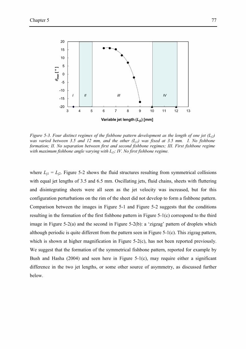
Chapter 5 77
where Lj1 = Lj2. Figure 5-2 shows the fluid structures resulting from symmetrical collisions
with equal jet lengths of 3.5 and 6.5 mm. Oscillating jets, fluid chains, sheets with fluttering
and disintegrating sheets were all seen as the jet velocity was increased, but for this
configuration perturbations on the rim of the sheet did not develop to form a fishbone pattern.
Comparison between the images in Figure 5-1 and Figure 5-2 suggests that the conditions
resulting in the formation of the first fishbone pattern in Figure 5-1(c) correspond to the third
image in Figure 5-2(a) and the second in Figure 5-2(b): a ‘zigzag’ pattern of droplets which
although periodic is quite different from the pattern seen in Figure 5-1(c). This zigzag pattern,
which is shown at higher magnification in Figure 5-2(c), has not been reported previously.
We suggest that the formation of the symmetrical fishbone pattern, reported for example by
Bush and Hasha (2004) and seen here in Figure 5-1(c), may require either a significant
difference in the two jet lengths, or some other source of asymmetry, as discussed further
below.
Figure 5-3. Four distinct regimes of the fishbone pattern development as the length of one jet (Lj2) was varied between 3.5 and 12 mm, and the other (Lj1) was fixed at 3.5 mm. I. No fishbone formation; II. No separation between first and second fishbone regimes; III. First fishbone regime with maximum fishbone angle varying with Lj2; IV. No first fishbone regime.
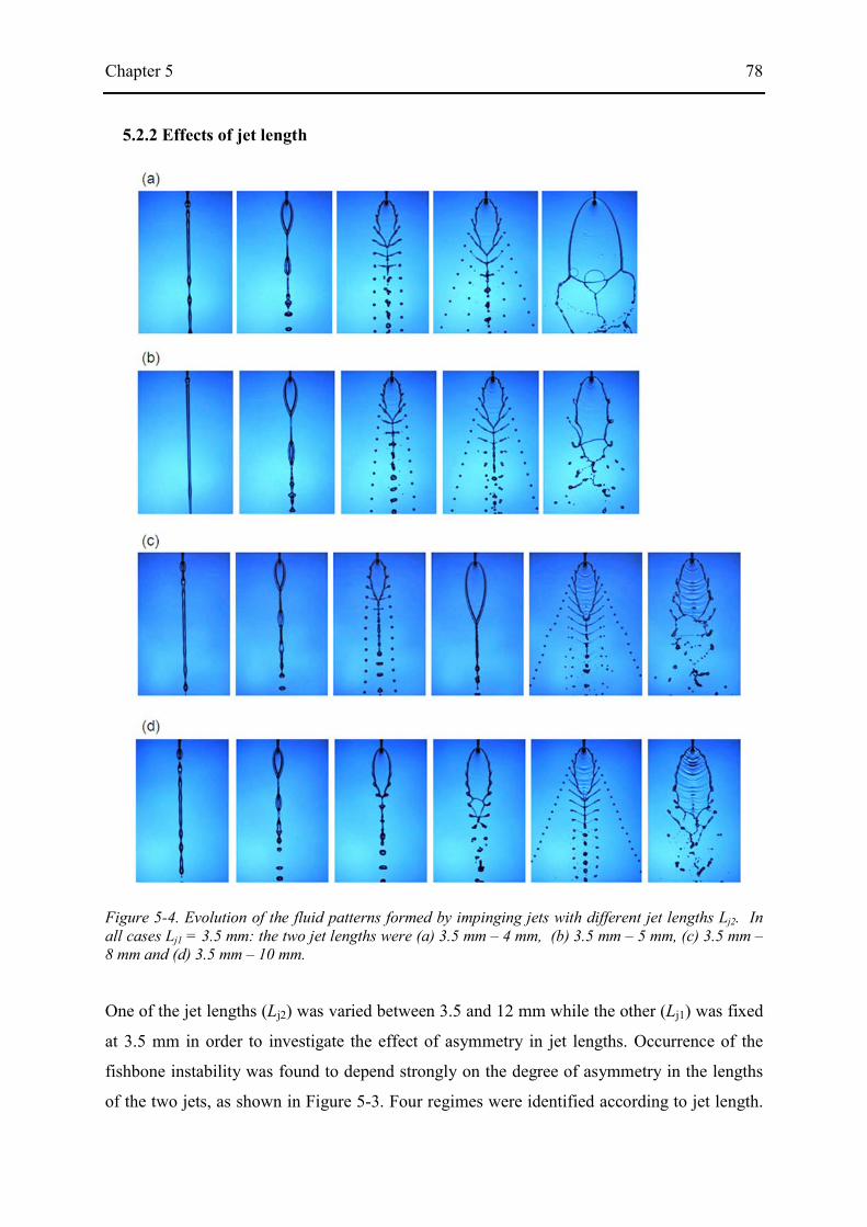
Chapter 5 78
5.2.2 Effects of jet length
One of the jet lengths (Lj2) was varied between 3.5 and 12 mm while the other (Lj1) was fixed
at 3.5 mm in order to investigate the effect of asymmetry in jet lengths. Occurrence of the
fishbone instability was found to depend strongly on the degree of asymmetry in the lengths
of the two jets, as shown in Figure 5-3. Four regimes were identified according to jet length.
Figure 5-4. Evolution of the fluid patterns formed by impinging jets with different jet lengths Lj2. In all cases Lj1 = 3.5 mm: the two jet lengths were (a) 3.5 mm – 4 mm, (b) 3.5 mm – 5 mm, (c) 3.5 mm –8 mm and (d) 3.5 mm – 10 mm.

Chapter 5 79
In regime I (~3.5 mm < Lj2 < ~4 mm) the collision was effectively symmetrical and no
fishbone pattern was generated. The flow patterns were as shown in Figure 5-2(a). In regime
II (~4 mm < Lj2 < ~5 mm) a well-defined fishbone pattern formed, which persisted with
increasing velocity, without an intermediate smooth sheet/chain pattern, until it entered a
violent flapping regime. Typical flow patterns are shown in Figure 5-4(a) and (b).
Regime III (~5 mm < Lj2 < ~10 mm) showed a similar progression of flow patterns to that
of regime II. But as discussed above and shown in Figure 5-1, the formation of a smooth fluid
sheet occurred between two distinct ‘fishbone’ regimes. At high values of Lj2 in regime III,
the overall pattern evolution proceeded in a similar way with increasing flow rate, except that
the first fishbone structure became far more sensitive to jet length than the second fishbone
structure (cf Figure 5-1 and Figure 5-4 (c)).
It is useful to introduce the concept of ‘fishbone angle’ to describe the degree of
development of the first fishbone structure. The fishbone angle can be defined as the angle (θ)
between the trajectories of the droplets on each side of the spine, as shown in Figure 5-5. The
maximum fishbone angle (θmax) is the value of θ when the flow structure is fully developed,
at the point just before it changes to the next regime (e.g. a smooth fluid sheet). Two
consecutive droplets in each stream are selected which are about to detach or have just
detached from the ligaments. The centres of area of these four droplets, determined by image
processing, are used to define the included angle. For example, the fishbone angle
(corresponding here to θmax) for the pattern shown in Figure 5-5 (a) (where Lj2 = 6.5 mm and
Lj1 = 3.5 mm) is 17°, whereas in Figure 5-5 (b) (where Lj2 = 8.5 mm and Lj1 = 3.5 mm) it is -
2°. The value of θmax can be reproducibly determined to better than 0.5°. The maximum
Figure 5-5. Definition of the fishbone angle as the angle between the trajectories of the droplets on each side of the fishbone structure. The maximum fishbone angle (MFA) is the largest value of this angle for a given fluid, as the flow is slowly increased. (a) θ =17°, (b) θ = -2°
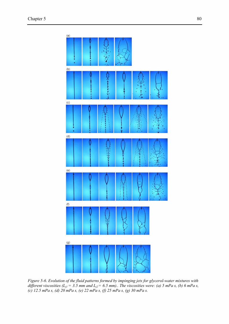
Chapter 5 80
Figure 5-6. Evolution of the fluid patterns formed by impinging jets for glycerol-water mixtures with different viscosities (Lj1 = 3.5 mm and Lj2 = 6.5 mm).. The viscosities were: (a) 5 mPa s, (b) 6 mPa s, (c) 12.5 mPa s, (d) 20 mPa s, (e) 22 mPa s, (f) 25 mPa s, (g) 30 mPa s.
Chapter 5 81
fishbone angle for the fluid with a viscosity of 10 mPa s is plotted against the variable jet
length Lj2 in Figure 5-5. The value of θmax in regime III decreased with increasing value of Lj1
over the range from ~7 to 9 mm, as the degree of asymmetry of the jets increased.
In regime IV (10 mm < Lj2 < 12 mm), small perturbations on the rim of the sheet were
observed but did not develop as the velocity was increased, and the first fishbone pattern did
not appear (as shown in Figure 5-4(d)). Instead, the fluid chain pattern changed, via a
fluttering sheet, directly to a second fishbone pattern with a regular internal spine, ligaments
and interior rows of drops.
5.2.3 Effects of viscosity
The viscosity of the fluid was varied between 4 and 30 mPa s for constant (asymmetric) jet
lengths of Lj2 = 6.5 mm and Lj1 = 3.5 mm, and had a marked effect on the flow patterns, as
shown in Figure 5-6. Fishbone patterns occurred only for viscosities between 6 and 25 mPa s.
Lower viscosity fluids atomised readily into random droplets at low flow velocity. For higher
viscosities, fluid chains and smooth single sheets persisted up to about 4 m s-1. For a viscosity
of 6 mPa s the first fishbone pattern appeared at 2.3 m s-1; it attained the largest value of θ at
12.5 mPa s, and was no longer seen for 22 mPa s. Figure 5-7 and Figure 5-8 show how the
maximum fishbone angle varied with increasing fluid viscosity from negative values (i.e
converging rows of drops) to positive values (diverging rows of drops) and then returned to
negative values. Second fishbone patterns were seen for viscosities from 10 to 28 mPa s and
the included angle varied in a similar way to the first.
The combined influences of viscosity and jet velocity are represented in Figure 5-9 in
terms of the values of Weber number and Reynolds number. In this graph a constant value of
Ohnesorge number (Oh = We1/2/Re) plots as a straight line through the origin and each set of
data points aligned in this way corresponds to results from a fluid with a single value of
viscosity. The first fishbone patterns appeared between the fluid chain and smooth single
sheet regime over a relatively narrow range within the region defined by 110 < Re < 290 and
6.8 < We1/2 < 10. The second fishbone regime lay within the range 105 < Re < 250 and 10 <
We1/2 < 11.3. No fishbone pattern was observed in this system when the Ohnesorge number
exceeded 0.1 (as the instability was resisted by fluid viscosity) or fell below 0.025 (as it was
resisted by fluid inertia).
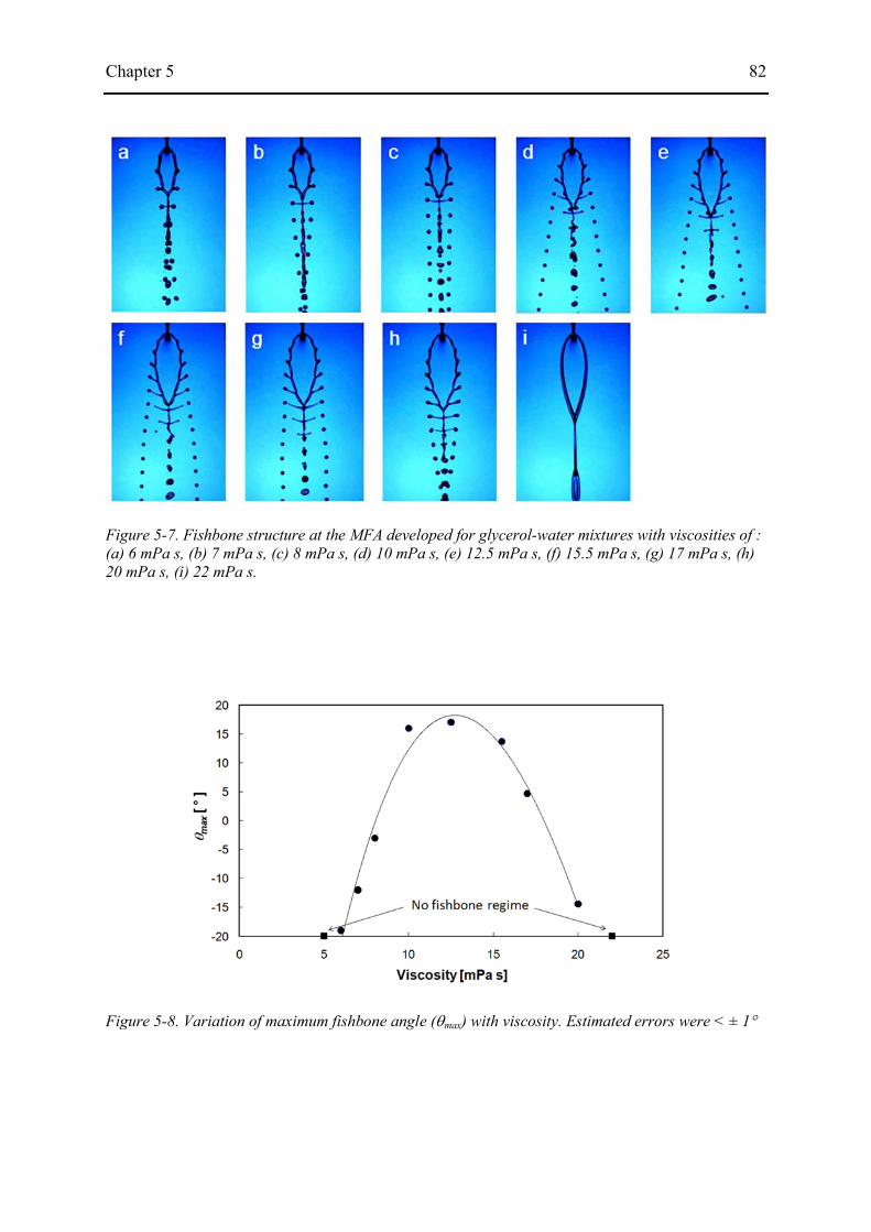
Chapter 5 82
Figure 5-7. Fishbone structure at the MFA developed for glycerol-water mixtures with viscosities of : (a) 6 mPa s, (b) 7 mPa s, (c) 8 mPa s, (d) 10 mPa s, (e) 12.5 mPa s, (f) 15.5 mPa s, (g) 17 mPa s, (h) 20 mPa s, (i) 22 mPa s.
Figure 5-8. Variation of maximum fishbone angle (θmax) with viscosity. Estimated errors were < ± 1°

Chapter 5 83
Figure 5-9. Regime diagram for glycerol-water mixtures, showing the relevant flow patterns in terms of Re and We1/2. A constant value of Ohnesorge number (Oh = We1/2/ Re) plots as a straight line through the origin. F1 corresponds to the first fishbone regime; F2 corresponds to the second fishbone regime.
Figure 5-10. Jet velocity and sheet dimensions corresponding to the fishbone structure at the point of maximum fishbone angle. Jet velocity and sheet dimensions corresponding to the fishbone structure at the point of maximum fishbone angle.
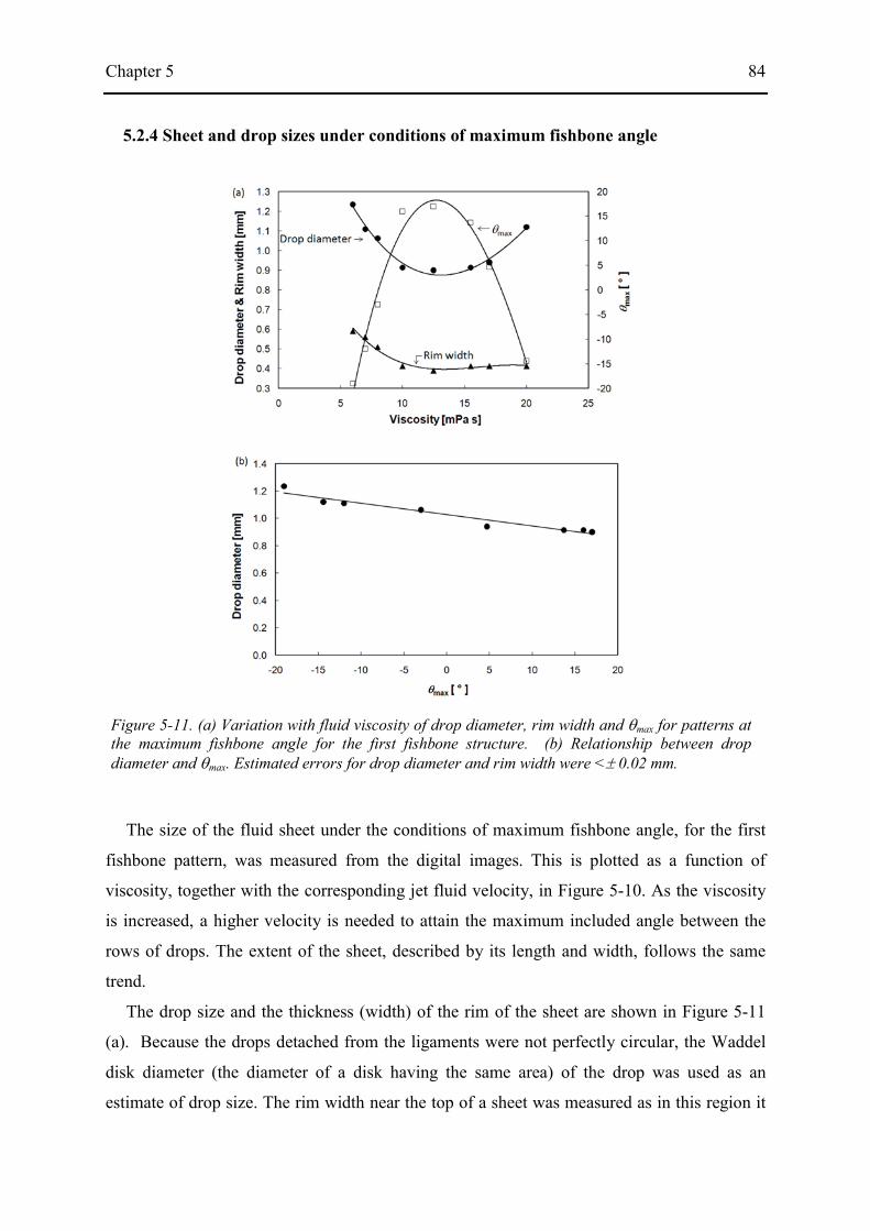
Chapter 5 84
5.2.4 Sheet and drop sizes under conditions of maximum fishbone angle
The size of the fluid sheet under the conditions of maximum fishbone angle, for the first
fishbone pattern, was measured from the digital images. This is plotted as a function of
viscosity, together with the corresponding jet fluid velocity, in Figure 5-10. As the viscosity
is increased, a higher velocity is needed to attain the maximum included angle between the
rows of drops. The extent of the sheet, described by its length and width, follows the same
trend.
The drop size and the thickness (width) of the rim of the sheet are shown in Figure 5-11
(a). Because the drops detached from the ligaments were not perfectly circular, the Waddel
disk diameter (the diameter of a disk having the same area) of the drop was used as an
estimate of drop size. The rim width near the top of a sheet was measured as in this region it
Figure 5-11. (a) Variation with fluid viscosity of drop diameter, rim width and θmax for patterns at the maximum fishbone angle for the first fishbone structure. (b) Relationship between drop diameter and θmax. Estimated errors for drop diameter and rim width were <± 0.02 mm.

Chapter 5 85
was relatively constant, since centripetal acceleration was smallest. The drop size and rim
width did not vary linearly with viscosity, unlike the trends seen for sheet size (Figure 5-10).
The rim width became smaller as the sheet expanded for viscosities from 5 to 12.5 mPa s and
then remained relatively constant from 12.5 to 20 mPa s. Figure 5-11(a) shows that the drops
associated with the highest θmax were the smallest; the drop size decreased linearly as θmax
increased (Figure 5-11b). Estimated errors for drop diameter and rim width were < ± 0.02mm.
5.2.5 Induction of the fishbone instability by external perturbation
Two methods were demonstrated by Bremond and Villermaux (2006) to induce the
fishbone instability by introducing external perturbation: by touching a small wire on to the
sheet rim, or by vibrating the nozzles at frequencies between 600 and 1000 Hz. Here, we
explored a further way to stimulate the fishbone instability, by externally disturbing one of
the two free liquid jets with a thin copper wire (200 µm diameter). Figure 5-12(a) shows the
fluid sheet formed by the symmetrical collision of two jets with the same length (Lj1 = Lj2 =
3.5 mm); no fishbone pattern is formed. With the wire touching one of the jets, the jet, and
hence the rim of the sheet, is perturbed, leading to fishbone instability which is, however, not
symmetrical. As shown in Figure 5-12(b) and (c), the pattern formed depends on the position
of the wire on the jet.
Figure 5-12. Observation of fishbone instability resulting from external perturbation by a thin wire touching one jet. η = 10 mPa s and Vj = 2.2 m s-1
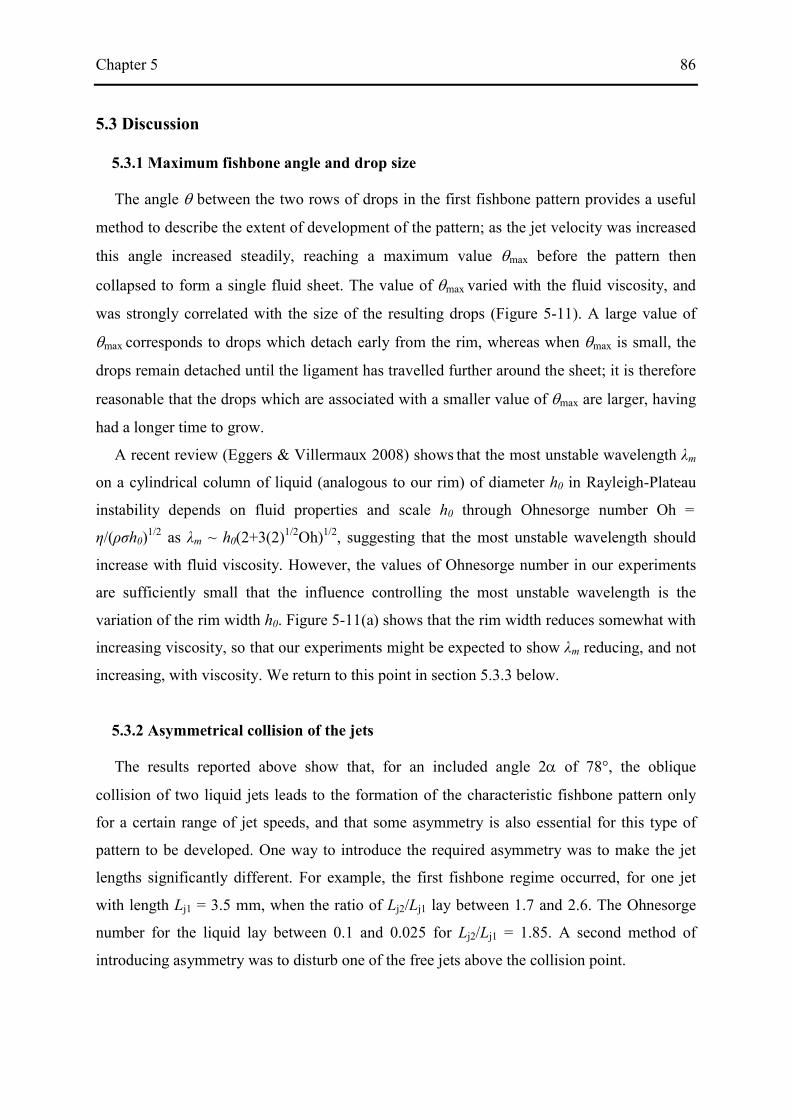
Chapter 5 86
5.3 Discussion
5.3.1 Maximum fishbone angle and drop size
The angle θ between the two rows of drops in the first fishbone pattern provides a useful
method to describe the extent of development of the pattern; as the jet velocity was increased
this angle increased steadily, reaching a maximum value θmax before the pattern then
collapsed to form a single fluid sheet. The value of θmax varied with the fluid viscosity, and
was strongly correlated with the size of the resulting drops (Figure 5-11). A large value of
θmax corresponds to drops which detach early from the rim, whereas when θmax is small, the
drops remain detached until the ligament has travelled further around the sheet; it is therefore
reasonable that the drops which are associated with a smaller value of θmax are larger, having
had a longer time to grow.
A recent review (Eggers & Villermaux 2008) shows that the most unstable wavelength λm
on a cylindrical column of liquid (analogous to our rim) of diameter h0 in Rayleigh-Plateau
instability depends on fluid properties and scale h0 through Ohnesorge number Oh =
η/(ρσh0)1/2 as λm ~ h0(2+3(2)1/2Oh)1/2, suggesting that the most unstable wavelength should
increase with fluid viscosity. However, the values of Ohnesorge number in our experiments
are sufficiently small that the influence controlling the most unstable wavelength is the
variation of the rim width h0. Figure 5-11(a) shows that the rim width reduces somewhat with
increasing viscosity, so that our experiments might be expected to show λm reducing, and not
increasing, with viscosity. We return to this point in section 5.3.3 below.
5.3.2 Asymmetrical collision of the jets
The results reported above show that, for an included angle 2α of 78°, the oblique
collision of two liquid jets leads to the formation of the characteristic fishbone pattern only
for a certain range of jet speeds, and that some asymmetry is also essential for this type of
pattern to be developed. One way to introduce the required asymmetry was to make the jet
lengths significantly different. For example, the first fishbone regime occurred, for one jet
with length Lj1 = 3.5 mm, when the ratio of Lj2/Lj1 lay between 1.7 and 2.6. The Ohnesorge
number for the liquid lay between 0.1 and 0.025 for Lj2/Lj1 = 1.85. A second method of
introducing asymmetry was to disturb one of the free jets above the collision point.

Chapter 5 87
The observation that significant asymmetry is needed to produce the fishbone pattern is not
consistent with the reports of Bush and Hasha (2004) who observed fishbone structures in the
symmetrical collision of jets of glycerol-water mixtures, with apparently identical jet lengths.
It is however possible that their fishbone patterns in fact resulted from asymmetric rather than
symmetrical collisions. Their published images suggest that the fishbone pattern was formed
in a plane rotated away from the normal to the plane containing the jets, because both nozzles
can be clearly seen in their pictures (reproduced in Figure 5-13), whereas only a single nozzle
is seen in side view (presumably with the other immediately behind it) in their images
showing the other flow regimes. We have tested this hypothesis by further investigating the
asymmetrical collision of jets with identical lengths in which the axes of the jets, originally
co-planar, were slightly displaced from the original plane in which they lay. The series of
images in Figure 5-14 was obtained in this way, for a viscosity of 10 mPa s with Lj2 = Lj1 =
6.5 mm and a jet velocity of 2.3 m s-1. Co-planar jets do not form a fishbone pattern, but
instead form a fluttering fluid sheet. Slight displacement of the jets so that their axes are no
longer co-planar but remain in vertical planes, however, does lead to fishbone patterns. As
shown in Figure 5-14(b) to (e), these patterns are rotated so that they do not lie normal to the
planes of the jets; in these images which have been formed with the optical axis normal to the
fluid sheet, both jets are visible forming a V-shape at the top of the frame, as they also are in
the images presented by Bush and Hasha (2004). Greater lateral displacement of the jets led
to a fuller development of the fishbone pattern with a higher included angle θ and greater
rotation of the plane of the pattern about the vertical. All the other images in this work were
generated with co-planar jets, and for these the fluid sheets and rows of drops were normal to
the jet plane: only a single jet/nozzle is visible in those images.
From our experiments the relationship between the maximum fishbone angle and the angle
by which the fluid sheet is rotated about the vertical axis is plotted in Figure 5-15. The value
of θmax was very sensitive to the degree of jet displacement and varied linearly with the
pattern rotation. We conclude that the fishbone instability can be induced by even slight
misalignment of the two jets, and that the extent of misalignment has a large effect on the
degree of development of the instability.
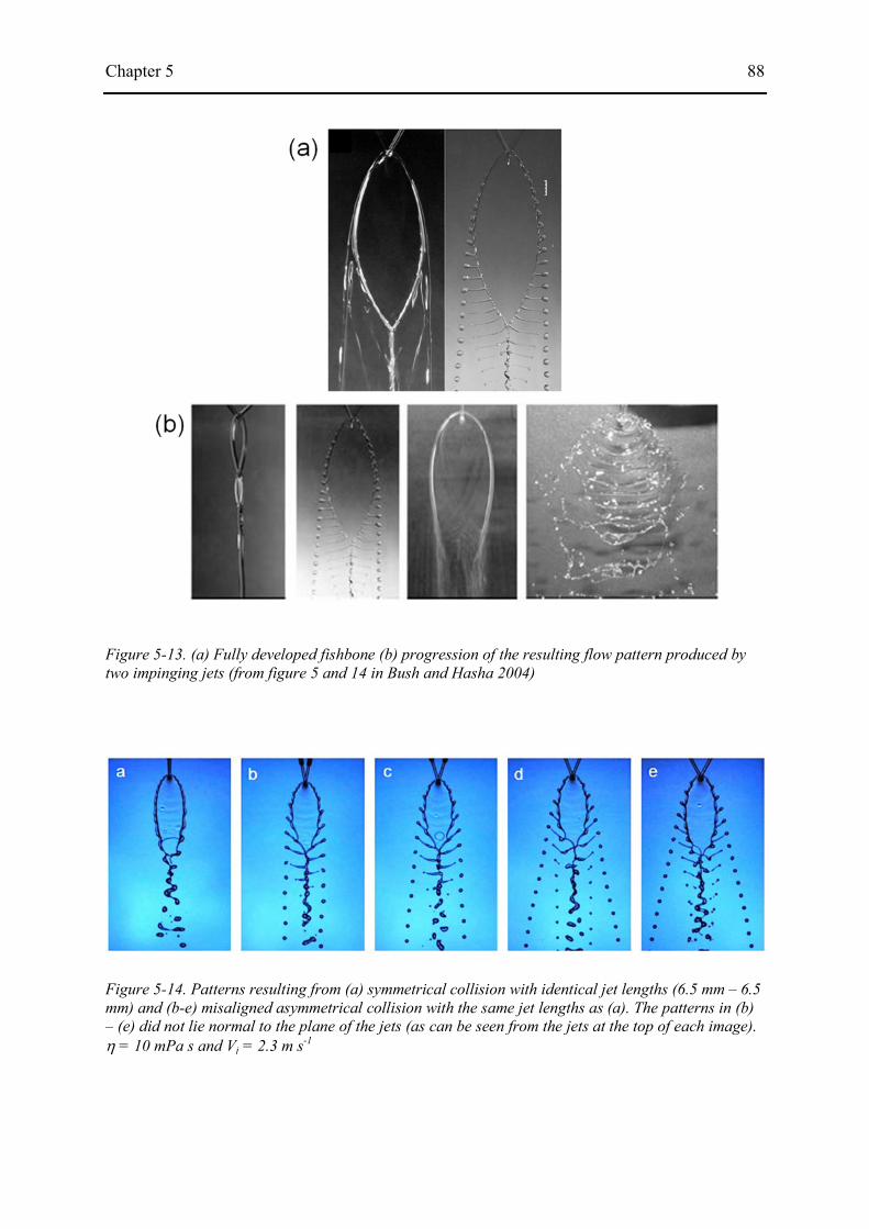
Chapter 5 88
Figure 5-14. Patterns resulting from (a) symmetrical collision with identical jet lengths (6.5 mm – 6.5 mm) and (b-e) misaligned asymmetrical collision with the same jet lengths as (a). The patterns in (b) – (e) did not lie normal to the plane of the jets (as can be seen from the jets at the top of each image). η = 10 mPa s and Vj = 2.3 m s-1
Figure 5-13. (a) Fully developed fishbone (b) progression of the resulting flow pattern produced by two impinging jets (from figure 5 and 14 in Bush and Hasha 2004)

Chapter 5 89
5.3.3 Fishbone instability
Bush and Hasha (2004) concluded that the fishbone pattern represents a rim-driven rather
than a sheet-driven instability, and explained that a Rayleigh–Plateau instability and a
centrifugal Rayleigh–Taylor instability were relevant to destabilisation of the rim and its
periodic atomisation. They reported that the spacing of their ligaments lay between 7 and 10
mm, and did not mention any dependence on the fluid properties although the viscosities of
their fluids ranged from 5 to 39.5 mPa s. A constant ligament spacing of this magnitude
would be broadly consistent with the wavelength of a Rayleigh–Plateau instability, which
would be 7.22 mm (= 4.51Dj) for their orifice radius of 0.8 mm. However, our results clearly
demonstrate that the spacing between the peaks on the rim, the resulting ligaments or the
detached droplets varies strongly with viscosity. Figure 5-16(a) shows that the instability on
the rim continues to grow not only in length, but also in spacing until a droplet becomes
detached from the ligament. The significant growth of the spacing along the rim is consistent
with the increase in the fluid velocity with azimuthal angle in the sheet (Choo & Kang 2002).
The spacing also varies with the viscosity, decreasing down to 12.5 mPa s at which θmax is
highest. There is then no significant difference over the range from 12.5 to 20 mPa s.
Bush and Hasha’s regime diagram is plotted on axes which differ by a factor of π/2 in Re
and 2/π2 in We from the values used in our regime diagram. In terms of our values of Re and
Figure 5-15 Variation of maximum fishbone angle with the angle by which the pattern is rotated, for misaligned asymmetrical jet collisions corresponding to Figure 13. Estimated errors were < ± 1°
Chapter 5 90
Figure 5-16. (a) Variation of spacing of the rim perturbation and drop formed from the rim, for fluids with different viscosities as shown. The broken line indicates a spacing of 4.51Dj. (b) Comparison between drop spacing and rim width for patterns with maximum fishbone angle, for fluids of different viscosities. (c) Evolution of rim thickness Dr with angular position around the rim for different systems. () 20 mPa s glycerol-water with 2a=78° (this work), () ethanol with 2α=89° [data from Bremond and Villermaux, 2006). Estimated errors for spacing were < ±0.1 mm.

Chapter 5 91
We, their fishbone regime would appears in a range 180 < Re < 760 and 13 < We1/2 < 30,
which differs significantly from our results for the first fishbone regime, for which 100 < Re
< 280 and 7 < We1/2 < 10 (reproduced in Figure 5-17).
If Rayleigh–Plateau instability is indeed responsible for rim break-up in the fishbone
pattern, the wavelength of the peak and ligament spacing should be a function of the rim
width rather than of the nozzle diameter. The upper line in Figure 5-16(b) shows the spacing
λ between droplets when the droplet pinches off, which reaches its peak value close to the
maximum fishbone angle for each viscosity. The lower line shows the minimum thickness of
the rim Dr, at the top of the sheet, which also corresponds to the maximum fishbone angle.
Both sets of data show the same trends, with a steep decrease at the lower viscosities and a
plateau from 12.5 to 20 mPa s. The changes in drop spacing and rim width with viscosity
shown in Figure 5-16(b) are consistent with the interpretation of break-up arising from the
Rayleigh-Plateau instability for the fluids studied. Although the break-up wavelength λm for a
fixed value of h0 would be expected to increases slightly with viscosity through its effect on
Figure 5-17 Regime diagram illustrating the observed dependence of flow structures emerging from the collision of laminar viscous jets on the governing dimensionless groups. Seven distinct regimes are delineated: , oscillating streams; *, sheets with disintegrating sheets; , fluid chains; +, fishbones; , spluttering chains; , disintegrating sheets; ×, violent flapping. Glycerol-water solutions with viscosities in the range of 1 to 94 cS were examined. (from Figure 11in Bush and Hasha 2006)
Chapter 5 92
Oh, it in fact decreases because the rim width h0 decreases strongly with viscosity. The ratio
between λm and h0 is constant, with λ = (9 ± 0.5) Dr. This ratio is significantly different from
the ratio of 4.51 expected for Rayleigh break-up of a jet, but it must be borne in mind that Dr
was measured at the thinnest region of the rim, and that it becomes much thicker away from
this point. Figure 5-16(c) shows measurements of the rim width as a function of angular
position around the rim for a glycerol-water mixture (viscosity 20 mPa s) with 2α = 78° and
for comparison, data from Bremond and Villermaux (2006) for ethanol with 2α = 89°. The
rim width increases to a maximum of about two and a half times the minimum value at the
top of the sheet. We suggest that these results are consistent with surface tension-driven,
Rayleigh-Plateau break-up, as proposed by Bush and Hasha (2004) and confirmed by
Bremond and Villermaux (2006).
5.3.4 What causes the fishbone pattern?
The origin of the initial perturbation on the rim of the sheet which grows and leads to the
fishbone instability over a finite range of velocity and viscosity has not been identified in
previous work. Dombrowski & Hooper (1964) observed that the patterns formed by the
collision of two laminar jets were not the same as those caused by two turbulent jets having
the same Reynolds number. They suggested that the mechanism of sheet disintegration was
independent of Reynolds number and was affected only by the velocity profile across the jet
and the angle of their impingement. From our experimental results we suggest that the rim
perturbation needed to induce the fishbone pattern may be initiated by the interaction of the
fluid from two jets with different velocity profiles. Three methods have been investigated in
this work to initiate the instability.
First, the perturbation can be initiated from the top of the sheet and develop along the sides
when the jets collide symmetrically with the same diameter and velocity but with different
free jet lengths, because under these conditions the two jets have different velocity profiles at
the point of impact. We can assume that the jets emerge from the relatively long nozzles with
a Poiseuille profile. After emergence the velocity profile relaxes, with increasing velocity
near the now free boundary and decreasing velocity on its axis. Choo & Kang (2007) recently
used laser Doppler velocimetry (LDV) to measure the velocity distribution in a 2.75 m s-1 jet
from a 1 mm diameter nozzle. At 10 mm from the nozzle end the velocity distribution was
significantly different from the original Poiseuille profile. They also showed that the velocity

Chapter 5 93
profile in the jet significantly affected the velocity distribution within the sheet formed by
collision of two such jets. Battal et al. (2003) also used LDV to show axial velocity relaxation
in a free water jet emerging from a 1.58 mm nozzle; the profile progressively relaxed from a
parabolic shape along the axis (reproduced in Figure 5-18).
As shown in Figure 5-3, the length of one jet needed to lie in the range from 6 to 9 mm for
the fishbone pattern to form when the other jet length was fixed at 3.5 mm. The extent of the
pattern also depended strongly on the asymmetry between the jet lengths. The critical role
played by the jet velocity profile for fishbone development is supported by the results shown
in Figure 5-19, which were obtained with very long jets (Lj2 = 18 mm and Lj1 = 10 mm). In
this case the ratio Lj2/Lj1 = 1.8, similar to the value for the case where Lj2 = 6.5 mm and Lj1 =
3.5 mm which gave well-developed fishbones. For these long jets, no fishbone pattern was
formed, presumably because the velocity profiles from the two jets were insufficiently
different to initiate the fishbone instability. These results suggest that for jets colliding
symmetrically, a certain difference in their velocity profiles is required to generate the
perturbation which leads to the fishbone pattern, although the underlying reasons for this
remain unclear.
A second method of inducing the perturbation is by asymmetrical collision of two jets
with identical parabolic velocity profiles. Collision of two jets with the same jet length but
with their axes displaced into different vertical planes produces similar effects to the
Figure 5-18 Velocity distribution in a pure water jet. Experimental data from LDV measurements at z = 1 mm(), 10.5 mm(), 35.5 mm(), and 100 mm(). Solid lines represents Computer simulation.(from Figure 6 in Battal et al. 2003)

Chapter 5 94
symmetrical collision of jets with different jet length, presumably because there is a local
difference between the velocity profiles in the collision zone. This phenomenon has been
discussed in section 5.3.2: the sheet formed is rotated so that it is not normal to the planes
containing the jets. When Bremond and Villermaux (2006) observed the periodic atomisation
of an ethanol sheet, they reported that it was slightly rotated in this way. Although they
proposed that a small velocity difference between the incident jets, of the order of 10 cm s-1,
was responsible for this, it also seems possible that it may have been due to asymmetrical
collision rather than to the velocity difference. This is because asymmetrical collision results
in the formation of a rotated sheet, whereas a symmetry argument can be used to suggest that
a velocity difference between perfectly aligned jets should not result in any rotation of the
sheet from the median plane of the jets.
Finally, external disturbance of one or both jets, even in a geometrically symmetrical
arrangement, can generate the perturbation needed to initiate the fishbone pattern, by
influencing the velocity profile. Vibrating the jets provides one example of this (Bremond &
Villermaux 2006). We have demonstrated that disturbing the surface of one jet with a thin
wire can also induce the fishbone instability, and suggest that it does this by altering the
velocity profile in the jet.
5.4 Conclusions
A wide range of patterns can be developed by the break-up of the fluid sheet formed by
the oblique collision of two jets. We have focused on the remarkably symmetrical ‘fishbone’
pattern composed of a regular succession of longitudinal ligaments and droplets and shown
Figure 5-19 Patterns formed by the symmetrical collision of impinging jets with jet lengths Lj1 = 10 mm and Lj2 = 18 mm.

Chapter 5 95
that this is observed only within a certain range of Reynolds and Weber numbers. The (Re,
We) regime we find for fishbones is lower than that reported previously and furthermore, the
pattern does not occur for completely symmetrical jet collisions: some asymmetry is essential.
This asymmetry can be introduced in various ways: by the use of different lengths of free jet,
by displacing the jets laterally, or by disturbing the surface of one jet. The velocity profile
within the jets at the point of impact plays a key role in the initiation of the instability on the
rim of the fluid sheet which then develops into the fishbone pattern. The influence of the
Ohnesorge number on the drop spacing was small, with the main effects of fluid viscosity
entering through the rim diameter. Variations in the sheet rim width and drop spacing with
fluid viscosity are consistent with the interpretation of the fishbone pattern we report as
representing a Rayleigh-Plateau instability of the rim.

Chapter 6 96
6. Collision of two liquid jets: II. Non-Newtonian fluid
6.1 Introduction
In the previous chapter we have explained the remarkably symmetrical fishbone pattern
composed of a regular succession of ligaments and droplets which was formed at lower
values of Re and We than had been previously reported. Furthermore, the pattern did not
occur for completely symmetrical jet collisions. Some asymmetry in the jet collision proved
to be essential in order to generate the symmetrical fishbone pattern. The fishbone pattern
suggests that there might be a close similarity between the generation and extension of
ligament from the rim and the production of a drop and ligament in inkjet printing. We
therefore extend our interest to non-Newtonian jet collision and attempt to answer research
question 2 – whether this phenomenon can be a useful tool to observe and characterise inter-
chain interaction in high speed extensional flow of polymer-containing non-Newtonian inks
so that one can assess the printability of the inks, without involving a print head.
In this chapter, experimental observations and analysis are presented for the formation and
atomisation of the fluid sheet created by obliquely colliding jets of viscoelastic fluids. Non-
Newtonian polystyrene solutions in diethyl phthalate and polyethylene oxide solutions in
glycerol-water mixture (60/40 % by weight), both polymers with various molecular weights,
were used to investigate the effects of viscoelasticity on the fluid patterns. Their fluid
properties have been described in section 4.2.1, and the experimental apparatus is essentially
the same as that used in chapter 5. In order to generate a symmetrical fishbone pattern,
asymmetric jet velocity profiles were produced by the use of differing jet lengths Lj1 and Lj2,
defined as the distances from the ends of the nozzles to the point of impact. In all the
experiments of this chapter Lj1 = 3.5 mm and Lj2 = 6.5 mm. The angle 2α between the axes of
the jets was fixed at 78°.
Sections 6.2.1 to 6.2.4 provide qualitative observations of the flow patterns formed by the
collision of two non-Newtonian liquid jets and the experimental results on the influence of
viscoelasticity on them. The jetting behaviours of the same fluids are shown in the next
Chapter 6 97
section., the effect of elasticity on the occurrence of the fishbone pattern and the variation of
θmax with polymer concentration are further discussed in section 6.3.1 and 6.3.2. Finally, the
correlation between θmax and jetting performance is studied in section 6.3.3.
6.2 Results
6.2.1 Qualitative observations
Figure 6-1 shows the evolution with increasing flow velocity of the flow patterns formed
by the collision of two jets of 0.02 wt% PS 110K in DEP. Several regimes can be identified,
as discussed for purely Newtonian fluids in the last chapter. The regimes shown in Figure 6-1
are typical of the behaviour of fluids with little or no elasticity. At the lowest speeds (not
shown) the jets merge into a single stream which then breaks up into a single row of drops by
Plateau-Rayleigh instability. At higher jet speed (Figure 6-1a) we see the formation of a
vertical chain of linked fluid sheets in which each thin oval film is orthogonal to its
neighbours. At a higher flow rate (b) the first oval sheet becomes larger. Small perturbations
on the rim of the sheet appear and gradually grow, leading to thickened regions which
collapse as they move further downstream (c). As the flow rate is further increased (d), the
Figure 6-1. Short duration flash images showing the evolution of the fluid sheets formed by impinging jets as jet velocities are increased: 0.02% PS 110K. Features: fluid chain (a, b); periodic atomisation(c, d); smooth single sheet (e); sheet with fluttering (f, g); disintegrating ruffled sheet (h); violent flapping (i, j).

Chapter 6 98
pattern takes the characteristic form of a fluid ‘fishbone’ composed of a fluid sheet, a series
of ligaments extending laterally from a central spine, and two diverging rows of detached
droplets. The ligaments become longer, and their extent depends on both the viscosity and
elasticity of the fluid. When the ligaments have become extended to their maximum length,
above a certain jet speed the pattern suddenly converts into a stable single sheet (Figure 6-1e)
which is larger than that formed at the lower speeds. At still higher speed it becomes unstable
again, breaking up into random droplets (f). As the jet velocity is increased further, the sheet
becomes ruffled, forming a disintegrating sheet with stable rim (g, h). Finally, at the highest
flow rates studied, violent flapping ensues (i, j).
With greater elasticity, the behaviour is different, as seen in Figure 6-2 for 0.4% PS 488K
in DEP. As the jet speed is increased, the system forms in turn: an oscillating single stream
(not shown), a fluid chain (a, b); a single sheet (c, d); a disintegrating sheet (e); a sheet with
fluttering (f); periodic atomisation with a ruffled sheet (g); and violent flapping (h). It should
be noted that no fluid fishbone structure is developed with this more elastic fluid. The
periodic atomisation from the ruffled sheet seen in Figure 6-2(g) is quite different from that
seen in Figure 6-1 and is produced at higher flow rates, above that which causes a fluttering
sheet.
Figure 6-2. Short duration flash images showing the evolution of the fluid sheets formed by impinging jets as jet velocities are increased: 0.4% concentration of PS 488K. Features: fluid chain (a, b); single sheet (c, d); disintegrating sheet (e); sheet with fluttering (f); periodic atomisation with ruffled sheet (g); violent flapping (h).

Chapter 6 99
Diagrams showing the flow structure regimes observed in these experiments for each PS
solution are presented in terms of the Weber number (We) and polymer concentration in
Figure 6-3. The Weber number (defined here by We = ρVj²Dj/σ where ρ and σ are the density
and equilibrium surface tension of the liquid respectively, Vj is the average velocity of flow
from a single needle and Dj is jet diameter) represents the ratio of inertial force to surface
tension force. The polymer concentration has been normalised with respect to the critical
concentration c* (as listed in Table 4-1). Although the polymer concentration above which
the fishbone pattern did not form varied considerably with molecular weight, when plotted in
terms of reduced concentration (c/c*) the regime diagrams became remarkably similar. The
value of We is essentially proportional to the square of the jet velocity, which ranged here
from ~1 to ~4 m s-1, because the addition of these small concentrations of polymer had little
effect on the density or equilibrium surface tension of the fluid. Figure 6-4 shows regime
plots for the PEO solutions. For the higher molecular weights (PEO 1M to PEO 5M) the plots
again lie close to a single master curve (Figure 6-4a), but for the lower molecular weights (e.g.
PEO 200k and PEO 300k) the reduced concentration above which the fishbone pattern was
suppressed varied significantly with molecular weight.
Figure 6-3. Regimes of flow pattern as a function of Weber number and polymer concentration for the solutions of PS in DEP. The black points represent the concentration for the transition between fluid chain and fishbone pattern, the red points for the transition between fishbone and single sheet and the blue points for the transition between single sheet and sheet with fluttering.
Chapter 6 100
6.2.2 Influence of viscoelasticity on the fishbone pattern
Figure 6-5 compares the detailed shapes of the ligaments formed in the fishbone regime
with different fluids. With the Newtonian glycerol–water mixture (Figure 6-5a) they were
relatively thick, with no fine filaments at their tips, whereas the viscoelastic solutions of 0.1
wt% PS 110K and 0.0004 wt% PEO 2M (Figure 6-5b and c) formed fine filaments before the
droplets were finally pinched off from the ends of the ligaments; these filaments were also
associated in some cases with the formation of small satellite drops.
Figure 6-4. Regimes of flow pattern as a function of Reynolds number and polymer concentration for the solutions of PEO in water/glycerol. The black points represent the reduced concentration for the transition between fluid chain and fishbone pattern, the red points for the transition between fishbone and single sheet and the blue points for the transition between single sheet and sheet with fluttering.

Chapter 6 101
Figure 6-6 shows the fully developed fishbone patterns (at the flow velocity which gave the
most widely spread streams of droplets) for PS 110K with different polymer concentrations.
At the lower concentrations (0.01 to 0.2 wt%), well-spread patterns were formed, but
development of the pattern was progressively hindered by the addition of polymer and it was
no longer seen at all for the 1 wt% solution. The extent of the fishbone pattern depended
strongly on the degree of viscoelasticity.
The ‘fishbone angle’ (θ ) between the two rows of drops is defined in the inset to Figure
6-7. Although this angle was introduced in work on Newtonian fluids in the previous chapter,
it also provides a useful method to describe the effects of fluid viscoelasticity on the flow
structure in the fishbone regime; as the jet velocity was increased this angle increased steadily,
reaching a maximum (θmax) beyond which a fishbone pattern could not be maintained (any
increase in jet velocity producing a single fluid sheet). The value of θmax varies with fluid
viscosity for Newtonian fluids and as shown in the present chapter it is also closely correlated
with fluid elasticity.
The effects of both the concentration and the molecular weight of the polymer on θmax
were studied. Figure 6-7 shows the variation of θmax with polymer concentration for solutions
of PS 110K, PS 210K and PS 488K. For these dilute solutions containing well-separated
polymer molecules, θmax might be expected to be independent of the polymer concentration.
However, while the value of θmax was effectively constant for concentrations below ~0.1 wt%
Figure 6-5. Details of ligament shapes and pinch–off regions: (a) Newtonian glycerol/water mixture (viscosity 12.5 mPa s); (b) 0.1 wt% PS 110K in DEP (10.4 mPa s); (c) 0.0004 wt% PEO 2M in glycerol/water (12.4 mPa s)
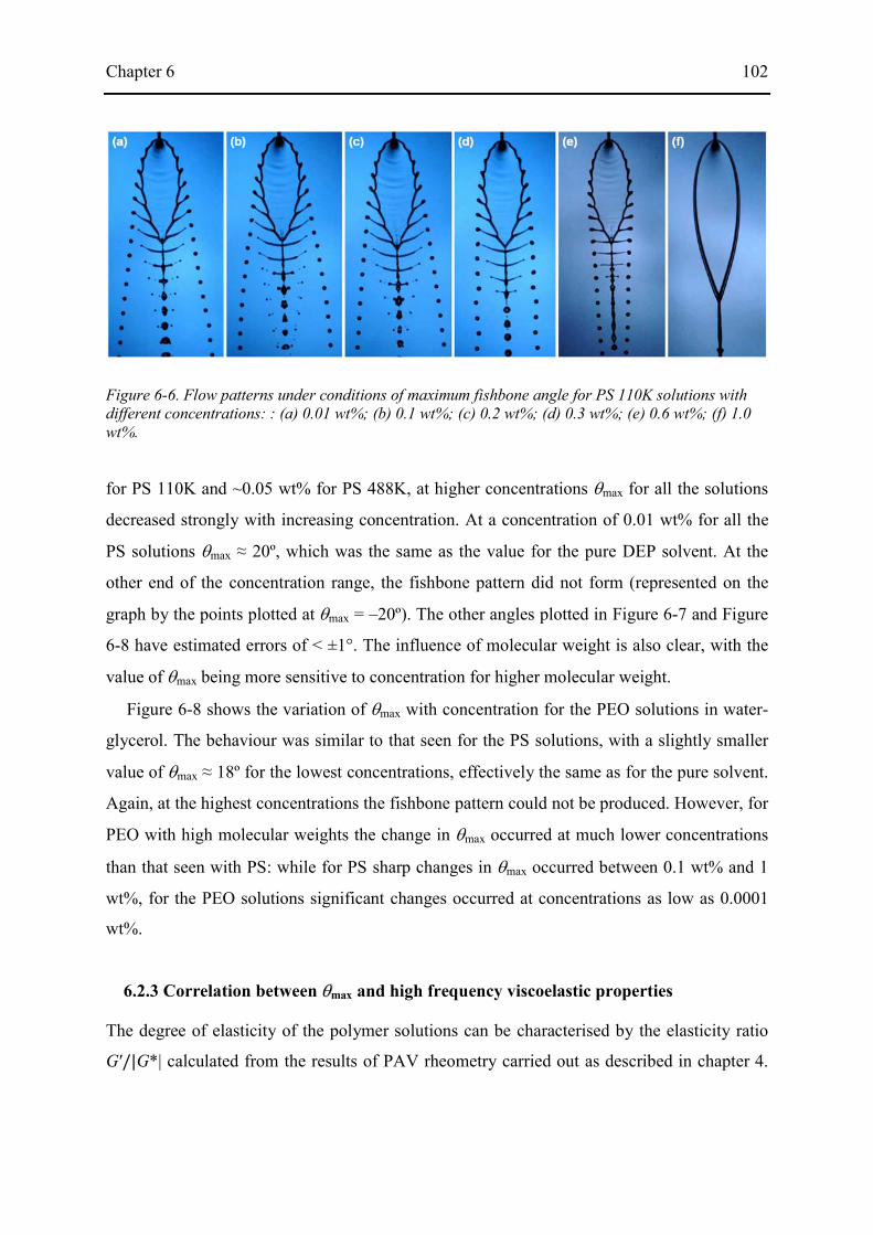
Chapter 6 102
for PS 110K and ~0.05 wt% for PS 488K, at higher concentrations θmax for all the solutions
decreased strongly with increasing concentration. At a concentration of 0.01 wt% for all the
PS solutions θmax ≈ 20º, which was the same as the value for the pure DEP solvent. At the
other end of the concentration range, the fishbone pattern did not form (represented on the
graph by the points plotted at θmax = –20º). The other angles plotted in Figure 6-7 and Figure
6-8 have estimated errors of < ±1°. The influence of molecular weight is also clear, with the
value of θmax being more sensitive to concentration for higher molecular weight.
Figure 6-8 shows the variation of θmax with concentration for the PEO solutions in water-
glycerol. The behaviour was similar to that seen for the PS solutions, with a slightly smaller
value of θmax ≈ 18º for the lowest concentrations, effectively the same as for the pure solvent.
Again, at the highest concentrations the fishbone pattern could not be produced. However, for
PEO with high molecular weights the change in θmax occurred at much lower concentrations
than that seen with PS: while for PS sharp changes in θmax occurred between 0.1 wt% and 1
wt%, for the PEO solutions significant changes occurred at concentrations as low as 0.0001
wt%.
6.2.3 Correlation between θmax and high frequency viscoelastic properties
The degree of elasticity of the polymer solutions can be characterised by the elasticity ratio
G′/|G*| calculated from the results of PAV rheometry carried out as described in chapter 4.
Figure 6-6. Flow patterns under conditions of maximum fishbone angle for PS 110K solutions with different concentrations: : (a) 0.01 wt%; (b) 0.1 wt%; (c) 0.2 wt%; (d) 0.3 wt%; (e) 0.6 wt%; (f) 1.0 wt%.
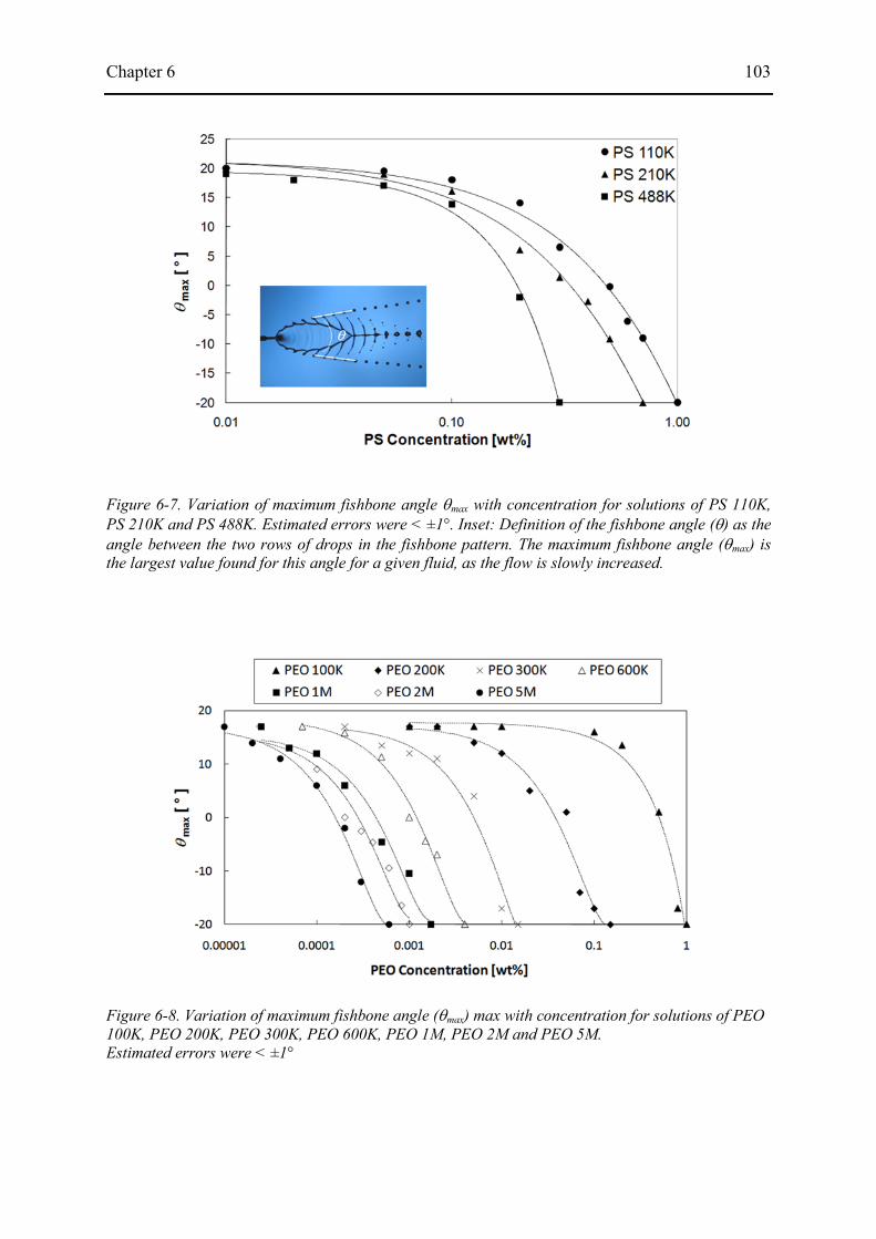
Chapter 6 103
Figure 6-7. Variation of maximum fishbone angle θmax with concentration for solutions of PS 110K, PS 210K and PS 488K. Estimated errors were < ±1°. Inset: Definition of the fishbone angle (θ) as the angle between the two rows of drops in the fishbone pattern. The maximum fishbone angle (θmax) is the largest value found for this angle for a given fluid, as the flow is slowly increased.
Figure 6-8. Variation of maximum fishbone angle (θmax) max with concentration for solutions of PEO 100K, PEO 200K, PEO 300K, PEO 600K, PEO 1M, PEO 2M and PEO 5M. Estimated errors were < ±1°

Chapter 6 104
Figure 6-9 (a-d) compares this ratio with θmax, as a function of polymer concentration for PS
110K, PS 488K, PEO 300K and PEO 1M solutions, respectively. Figure 6-9 (e, f) shows
G′/|G*| as a function of reduced concentration c/c* for all the PS and PEO solutions,
respectively. The ratio G′/|G*| was calculated at f = 1 kHz because the droplets were
detached from their ligaments in the fishbone pattern at intervals of ~1 ms. It is evident that
for all the solutions there is a strong correlation between θmax and the elasticity described in
this way. All of the solutions show a decrease in θmax as the elasticity modulus (G′) increased,
Figure 6-9. Maximum fishbone angle (θmax) and elasticity ratio G'/|G*| plotted against concentration for (a) PS 110K; (b) PS 488K; (c) PEO 300K; (d) PEO 1M, and G'/|G*| as a function of reduced concentration (c/c*) for (e) PS solutions; (f) PEO solutions.
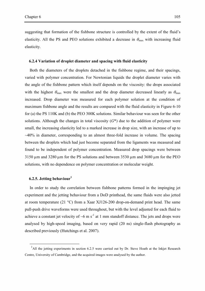
Chapter 6 105
suggesting that formation of the fishbone structure is controlled by the extent of the fluid’s
elasticity. All the PS and PEO solutions exhibited a decrease in θmax with increasing fluid
elasticity.
6.2.4 Variation of droplet diameter and spacing with fluid elasticity
Both the diameters of the droplets detached in the fishbone regime, and their spacings,
varied with polymer concentration. For Newtonian liquids the droplet diameter varies with
the angle of the fishbone pattern which itself depends on the viscosity: the drops associated
with the highest θmax were the smallest and the drop diameter decreased linearly as θmax
increased. Drop diameter was measured for each polymer solution at the condition of
maximum fishbone angle and the results are compared with the fluid elasticity in Figure 6-10
for (a) the PS 110K and (b) the PEO 300K solutions. Similar behaviour was seen for the other
solutions. Although the changes in total viscosity (G*) due to the addition of polymer were
small, the increasing elasticity led to a marked increase in drop size, with an increase of up to
~40% in diameter, corresponding to an almost three-fold increase in volume. The spacing
between the droplets which had just become separated from the ligaments was measured and
found to be independent of polymer concentration. Measured drop spacings were between
3150 µm and 3280 µm for the PS solutions and between 3530 µm and 3680 µm for the PEO
solutions, with no dependence on polymer concentration or molecular weight.
6.2.5. Jetting behaviour1
In order to study the correlation between fishbone patterns formed in the impinging jet
experiment and the jetting behaviour from a DoD printhead, the same fluids were also jetted
at room temperature (21 °C) from a Xaar XJ126-200 drop-on-demand print head. The same
pull-push drive waveforms were used throughout, but with the level adjusted for each fluid to
achieve a constant jet velocity of ~6 m s-1 at 1 mm standoff distance. The jets and drops were
analysed by high-speed imaging, based on very rapid (20 ns) single-flash photography as
described previously (Hutchings et al. 2007).
1All the jetting experiments in section 6.2.5 were carried out by Dr. Steve Hoath at the Inkjet Research
Centre, University of Cambridge, and the acquired images were analysed by the author.

Chapter 6 106
In order to examine the correlation between θmax and the performance of each fluid in a drop-
on-demand print head, the maximum ligament length (MLL) was measured from an image
captured at the point at which the jets had just detached from the nozzle plane. MLL is one of
the most important parameters which determines the printability of a fluid. Many printers
operate with about 1 mm stand-off distance, so that 1 mm is the maximum practical ligament
length for successful printing, although a maximum length of 0.4 to 0.6 mm might be
preferable for better print quality. Figure 6-11 (a) and (b) shows typical images of jets formed
from a dilute solution (0.01 wt% PS 110K in DEP) and from a solution close to the limit of
printability (0.4 wt% PS 110K). Once jets become detached from the nozzle plate they will
eventually either collapse to form a single drop or break up into multiple satellites; in extreme
cases they may never detach from the nozzle plate, as shown for a higher polymer
Figure 6-10. Dependence of drop diameter and elasticity ratio G'/|G*| on concentration for PS 110K solutions.

Chapter 6 107
concentration (1 wt% PS 110K) in Figure 6-11 (c). Long ligaments that do not become
detached may subsequently retract fully into the nozzle, while for even higher polymer
concentrations the fluid may never emerge from the nozzle.
Figure 6-11. Examples of jets emitted from a drop-on-demand printhead: (a) dilute polymer solution (0.01% PS 110K); (b) more concentrated solution which still forms detached jets (0.4% PS 110K); (c) even more concentrated solution for which the jets do not detach (1% PS 110K). Scale bar: 100 µm. (Captured by Dr. Steve Hoath)
Chapter 6 108
6.3 Discussion
6.3.1 Effect of elasticity on the occurrence of the fishbone pattern
For Newtonian fluids, the occurrence of the fishbone pattern has been shown in Figure 5-8
to depend markedly on viscosity. For example, in experiments with glycerol–water solutions
with viscosities between 4 and 30 mPa s, fishbones were only formed for viscosities between
6 and 22 mPa s, and θmax varied strongly with viscosity (0.025 < Oh < 0.1). The first
fishbone pattern appeared at 6 mPa s, was best developed with the highest value of θmax
between 10 and 15 mPa s, and disappeared for viscosities > 22 mPa s. The results presented
here show that the fishbone pattern also depends strongly on the elasticity of the fluid and
that the development of this structure can be suppressed by relatively small concentrations of
polymer, as shown in Figure 6-3 and Figure 6-4. While θmax was effectively the same as that
for the pure solvent at very low polymer concentrations, for both PS and PEO solutions
(Figure 6-7 and Figure 6-8) it decreased with increasing polymer concentration. There was a
strong correlation between the elasticity as measured by high-frequency rheometry and the
value of θmax (Figure 6-9). The viscosity and the dynamic surface tension for the surface age
relevant to the fishbone patterns in these fluids varied little, and it is therefore reasonable to
conclude that the fluid elasticity, as quantified by the ratio (G′/|G*|), controls the value of
θmax for these PS and PEO solutions.
The effects on the flow structure of adding polymer are most clearly seen in the context of
the periodic structure of the fishbone, which consists of a fluid sheet bounded by a thicker
rim, regularly spaced ligaments and droplets formed by the break-up of the rim. As discussed
by Cooper-White et al. (2002) and Tirtaatmadja et al. (2006), the early stage of droplet
formation is independent of the elasticity of the liquid as the dynamics are dominated by a
balance between inertial and capillary forces. But, at later stages of ligament growth, as the
polymer coils become extended, the presence of elastic stress influences the break–off length
and time (Tuladhar & Mackley 2008). Similar behaviour is also observed in the generation of
drops in ink-jet printing (Hoath et al. 2009), where droplet break-off is retarded and a notably
thinner ligament forms than from a Newtonian fluid. Similar phenomena were seen in the
fishbone structure when the ligaments were fully stretched (Figure 6-5). The timescales
involved in ligament growth can be estimated from the flow velocity and dimensions of the
sheet. The length of the sheet rim in the first fishbone pattern was typically ~20 mm, and the
speed of flow about 2.5 m s-1, which suggests a transit time from top to bottom of the sheet of

Chapter 6 109
~8 ms. This is much longer than the Zimm times listed in Table 4-1 and 4-2 for almost all the
polymers. Tirtaatmadja et al. (2006) have measured relaxation times for a range of PEO
solutions in glycerol-water with molecular weights between 3 × 10⁵ and 5 × 10⁶, from
experiments involving the formation and detachment of drops from thinning ligaments. They
reported that the effective relaxation times in these thinning filament experiments were up to
ten times the Zimm relaxation time, but the concentrations they used were substantially
higher than those used in our work: up to (c/c*) = 0.5. In contrast, we observed a major
influence of elasticity for (c/c*) below 0.01, for several of the PEO solutions (Figure 6-8)
which suggests that even at these concentrations the solutions were not effectively ‘dilute’.
Data from Tirtaatmadja et al. (2006) and other suggests that at these low concentrations the
relaxation times would not be expected to be significantly greater than the Zimm time. We
must conclude either that the flow pattern is being influenced by phenomena on a very much
shorter timescale than that of fluid motion around the rim (~10 ms), and thus closer to the
Zimm times of these polymers, or that for some reason the effective relaxation times in this
experiment are much greater than the Zimm time, even for dilute solutions. Tirtaatmadja et al.
(2006) commented that their own results for PEO did not depend significantly on the
presence of dynamic surface tension effects, which is also the case for all our results.
6.3.2 Variation of θmax with polymer concentration
The maximum fishbone angle θmax may prove useful to characterise the degree of fluid
elasticity, since we are able to deduce the presence of polymer interactions within the fluid in
terms of a reduction of the maximum fishbone angle as in Figure 6-7 and Figure 6-8, and also
an increased drop diameter as in Figure 6-10. The value of θmax reflects the time taken for the
drops to detach from the ligaments. A high value of θmax corresponds to drops which detach
early from the rim, whereas when θmax is small, the drops remain attached until the ligament
has travelled further around the edge of the sheet. This is consistent with the fact that the
drops which are associated with a smaller value of θmax are larger, as they will have been
growing for a longer time.
Figure 6-3 and Figure 6-4 suggest that for the PS solutions, and for the PEO solutions of
higher molecular weight, the effects of the polymer can be directly correlated with the
reduced concentration (c/c*), although this is not true for PEO with low molecular weights.
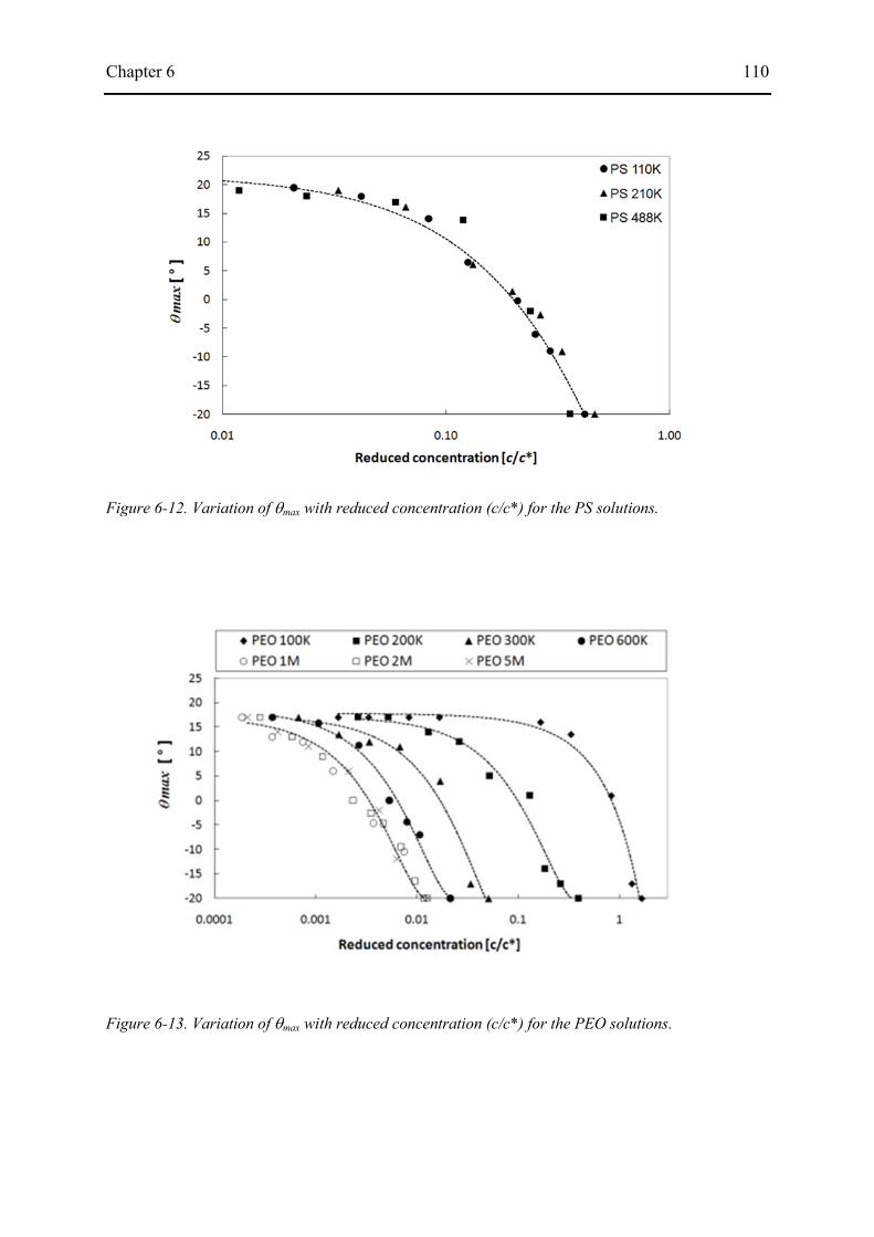
Chapter 6 110
Figure 6-12. Variation of θmax with reduced concentration (c/c*) for the PS solutions.
Figure 6-13. Variation of θmax with reduced concentration (c/c*) for the PEO solutions.

Chapter 6 111
Figure 6-12 and Figure 6-13 show plots of θmax against reduced concentration for these
polymers which demonstrate the same result: for PS and PEO with high molecular weight the
data lie in each case on a single master curve. We can conclude that at least for polystyrene in
a good solvent (DEP) over the range of molecular weight explored here, the value of θmax is a
universal function of the reduced concentration, regardless of the molecular weight and the
absolute polymer concentration. It is possible that the fishbone structure resulting from
oblique jet impact can be used, via the value of θmax, to identify the transition of a polymer
solution in a highly extended state from the dilute regime to the semi-dilute regime. In Figure
6-12, the value of θmax for concentrations below c/c* ≈ 0.05 is the same as that of pure DEP,
which is a Newtonian fluid. We infer from this that polymer chain interactions are negligible
at these concentrations and that the PS solutions below c/c* ≈ 0.05 can be classified as dilute
solutions. In contrast for c/c* > ~0.05 molecular interactions begin to influence the fishbone
pattern as droplet detachment becomes inhibited and the value of θmax falls. The entanglement
of polymer chains in the semi-dilute regime above c/c* ≈ 0.4 may prevent rim perturbations
from growing, resulting in the production of a smooth single sheet without atomisation.
These results are in good agreement with the results of Clasen et al. (2006) on filament
stretching of solutions in DEP of PS with much higher molecular weight.
The PEO solutions exhibit a more complex response, as shown in Figure 6-13. The data
for PEO 1M, PEO 2M and PEO 5M fall on to one master curve, as observed for the PS
solutions. At reduced concentrations c/c* < 0.0002 θmax has similar values to that for the pure
glycerol-water solvent. For higher concentrations θmax falls and the fishbone pattern is
completely suppressed above c/c* ≈ 0.01. This c/c* threshold is similar to that found for high
molecular weight PEO filament thinning behaviour by Tirtaatmadja et al (2006). However,
the data for PEO with molecular weight below 106 do not fall on the same curve, and show a
much stronger influence of molecular weight.
6.3.3 Correlation of θmax with jetting performance
The previous section has demonstrated that the elasticity of the fluid, as measured by high-
speed rheometry, is correlated with the value of θmax. Increasing elasticity results in a
decrease in θmax. Figure 6-14 compares the values of maximum ligament length as defined
above with the values of θmax for solutions of PS 110K, PS 210K, and PS 488K in DEP as a
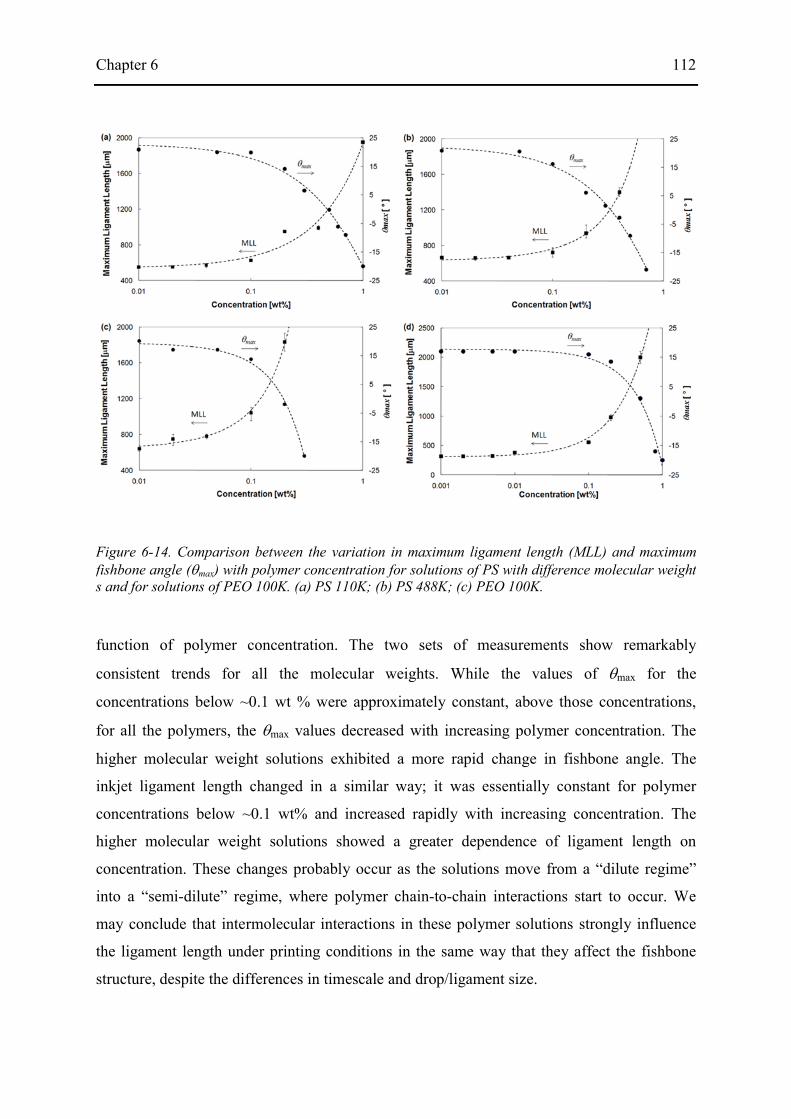
Chapter 6 112
function of polymer concentration. The two sets of measurements show remarkably
consistent trends for all the molecular weights. While the values of θmax for the
concentrations below ~0.1 wt % were approximately constant, above those concentrations,
for all the polymers, the θmax values decreased with increasing polymer concentration. The
higher molecular weight solutions exhibited a more rapid change in fishbone angle. The
inkjet ligament length changed in a similar way; it was essentially constant for polymer
concentrations below ~0.1 wt% and increased rapidly with increasing concentration. The
higher molecular weight solutions showed a greater dependence of ligament length on
concentration. These changes probably occur as the solutions move from a “dilute regime”
into a “semi-dilute” regime, where polymer chain-to-chain interactions start to occur. We
may conclude that intermolecular interactions in these polymer solutions strongly influence
the ligament length under printing conditions in the same way that they affect the fishbone
structure, despite the differences in timescale and drop/ligament size.
Figure 6-14. Comparison between the variation in maximum ligament length (MLL) and maximum fishbone angle (θmax) with polymer concentration for solutions of PS with difference molecular weight s and for solutions of PEO 100K. (a) PS 110K; (b) PS 488K; (c) PEO 100K.

Chapter 6 113
These results suggest that the observation of the interaction of colliding continuous jets
may be useful to obtain information which is relevant to the dynamics of drop formation nd
jet break-up in inkjet printing. From measurements of θmax for ink formulations containing
different concentrations of polymer, it should be possible to identify the level at which
viscoelastic effects will significantly affect jettability. The method might thus be used, after
suitable calibration experiments, as a guide to the maximum polymer content in fluids
intended for inkjet printing.
6.4 Conclusions
Elasticity has a strong effect on the formation and fragmentation of the fluid sheet formed
by the oblique collision of two jets. Fluids with low elasticity show similar break-up patterns
to those seen with a Newtonian fluid, including, for certain conditions, the formation of the
distinctive ‘fishbone’ pattern. The effect of increasing elasticity is to change the geometry
and eventually completely suppress the fishbone pattern, in a similar manner to the effect of
increasing the viscosity of a Newtonian fluid. As the elasticity of the fluid was increased, the
maximum angle defined by the fluid fishbone structure decreased, the size of the droplets
detached from the ligament increased, but the spacing of the ligaments remained unchanged.
The angle defined by the fishbone pattern θmax correlates closely with the degree of
elasticity as defined by the storage modulus (G′) of the solution, measured at high frequency
by piezoelectric axial vibrator rheometry. It is suggested that the occurrence and geometry of
fluid fishbone patterns can be used to detect and to some extent quantify elasticity in polymer
solutions in high-speed extensional flow.
Finally, we suggest that information about the printability of a viscoelastic (e.g., polymer-
containing) fluid can be obtained by observation of the fishbone structure, since these
patterns can be used to distinguish viscoelastic regimes in terms of degree of polymer dilution.
Good correlation is found between the maximum fishbone angle and the maximum ligament
length measured in jetting experiments from a DoD printhead, which suggests that the
fishbone phenomenon may provide a simple and useful tool to explore the upper limit of
polymer concentration in ink jet printing fluids.
Chapter 7 114
7. Drop impact dynamics: I. Newtonian fluid
7.1 Introduction
This chapter aims to provide experimental measurements of the dynamic behaviour of
liquid drops deposited on to non-porous surfaces and identify key parameters affecting the
drop impact process. The High-speed imaging system and the imaging processing technique
described in chapter 4 has been used to analyse the impact and spreading of 28 µm drops of
diethyl phthalate as a model Newtonian fluid on to smooth glass surfaces with varied
wettability at velocities from 3 to 8 m s-1, under conditions representative of drop-on-demand
inkjet printing. Highly wettable as-received ITO-coated, partially wettable corona-treated
ITO-coated and non-wettable PTFE-coated glass slides were used as models substrates.
The chapter begins with showing the results on jetting behaviour and drop generation in
section 7.2.1. The experimental observation of impact is provided in section 7.2.2 in order to
explore the full range of drop motion from the earliest stages of impact and spreading to
longer-term wetting and the final equilibrium state. Effects of various parameters which are
possibly affecting drop impact process are systematically investigated over sections 7.2.3 to
7.2.5.
Overall drop impact process is then discussed in section 7.3.1 and the key parameters
influencing it are identified. In the next section the predictions of analytical models for drop
spreading which have been reviewed in chapter 2 are compared with experimental
measurements of the maximum spreading factor of section 7.2. Section 7.3.3 shows
correlation between the deposition dynamics over the whole range of timescales of these
small drops, and the data for the much larger, mm-sized drops studied in much previous work.
Research questions 4 to 6 are addressed in this chapter. Study on this drop impact process
will continue in chapter 8 for polymer-containing, non-Newtonian model fluids.

Chapter 7 115
7.2 Results
7.2.1 Jetting behaviour and drop generation
Fluid flow in an inkjet print head is affected by the acoustic response to pressure waves
induced in the fluid by piezoelectric actuators. Since the displacement of the piezoelectric
actuator is proportional to the applied electric field, an increase in voltage amplitude results
in larger induced pressure waves and fluid accelerations in the nozzle chamber, and hence
faster drop speed and larger drop diameter. Figure 7-1 shows the influence of the input
voltage amplitude between 70 and 150 V on the speed and diameter of the DEP drops. The
shape of the drive waveform for drop eject has been shown in Figure 4-10. The speed of the
main drop was measured at a distance between 0.5 mm and 0.8 mm from the nozzle plate.
Figure 7-1. Influence of voltage amplitude of driving pulse on the speed and diameter of ejected DEP drops. Pulse duration is fixed at 5 µs.
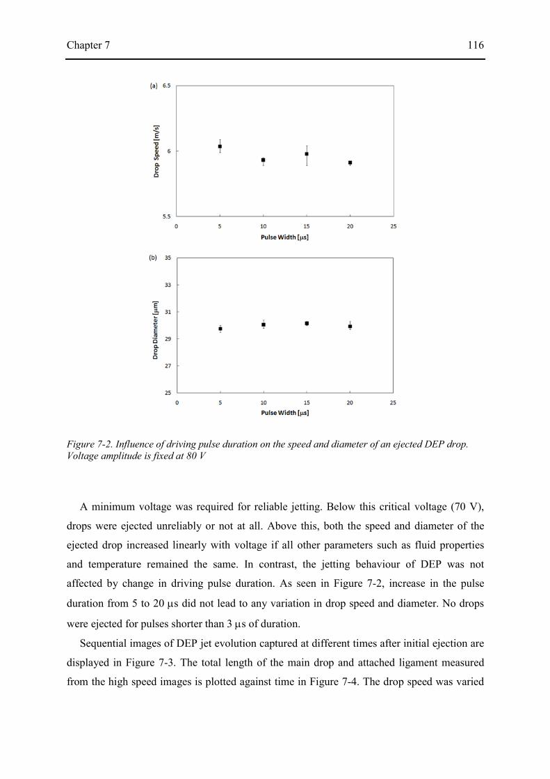
Chapter 7 116
A minimum voltage was required for reliable jetting. Below this critical voltage (70 V),
drops were ejected unreliably or not at all. Above this, both the speed and diameter of the
ejected drop increased linearly with voltage if all other parameters such as fluid properties
and temperature remained the same. In contrast, the jetting behaviour of DEP was not
affected by change in driving pulse duration. As seen in Figure 7-2, increase in the pulse
duration from 5 to 20 µs did not lead to any variation in drop speed and diameter. No drops
were ejected for pulses shorter than 3 µs of duration.
Sequential images of DEP jet evolution captured at different times after initial ejection are
displayed in Figure 7-3. The total length of the main drop and attached ligament measured
from the high speed images is plotted against time in Figure 7-4. The drop speed was varied
Figure 7-2. Influence of driving pulse duration on the speed and diameter of an ejected DEP drop. Voltage amplitude is fixed at 80 V
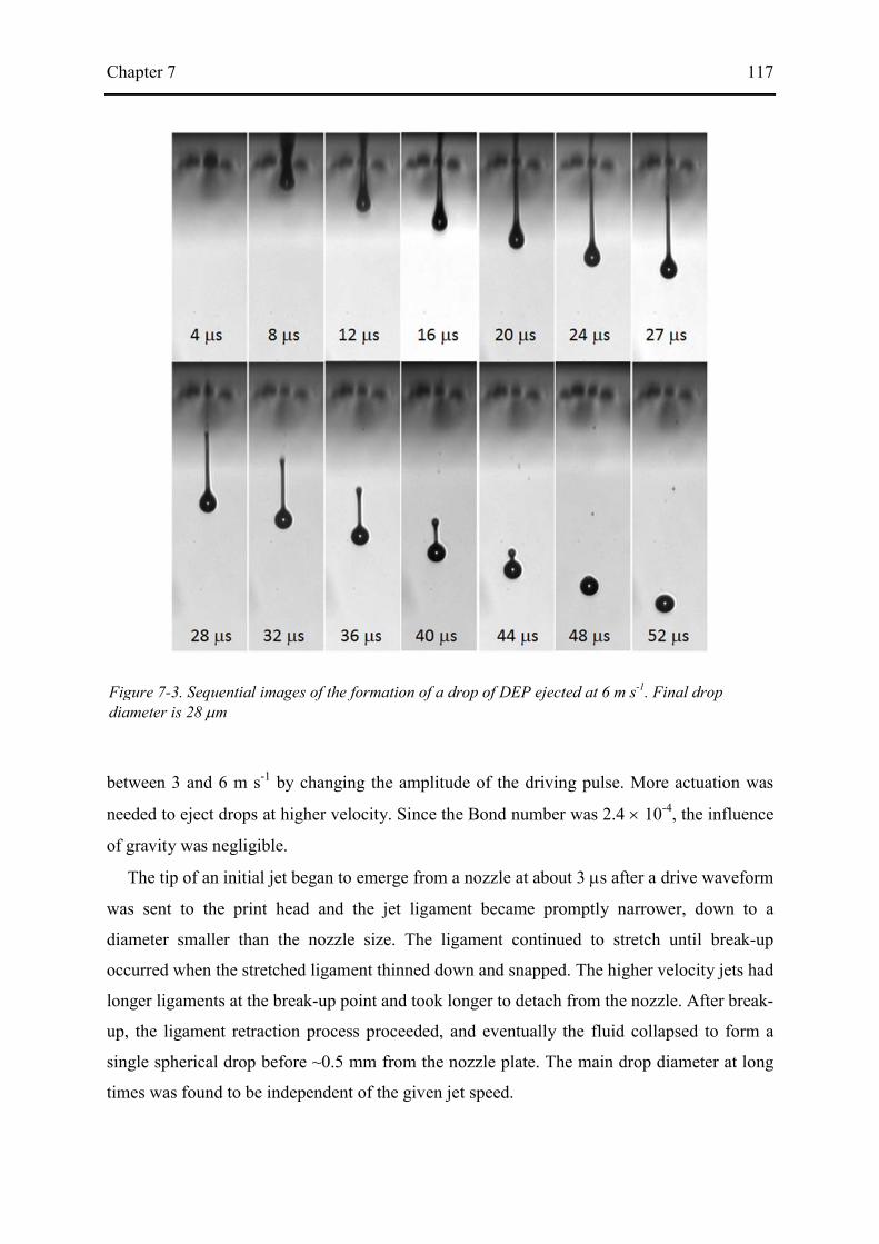
Chapter 7 117
between 3 and 6 m s-1 by changing the amplitude of the driving pulse. More actuation was
needed to eject drops at higher velocity. Since the Bond number was 2.4 × 10⁻⁴, the influence
of gravity was negligible.
The tip of an initial jet began to emerge from a nozzle at about 3 µs after a drive waveform
was sent to the print head and the jet ligament became promptly narrower, down to a
diameter smaller than the nozzle size. The ligament continued to stretch until break-up
occurred when the stretched ligament thinned down and snapped. The higher velocity jets had
longer ligaments at the break-up point and took longer to detach from the nozzle. After break-
up, the ligament retraction process proceeded, and eventually the fluid collapsed to form a
single spherical drop before ~0.5 mm from the nozzle plate. The main drop diameter at long
times was found to be independent of the given jet speed.
Figure 7-3. Sequential images of the formation of a drop of DEP ejected at 6 m s-1. Final drop diameter is 28 µm
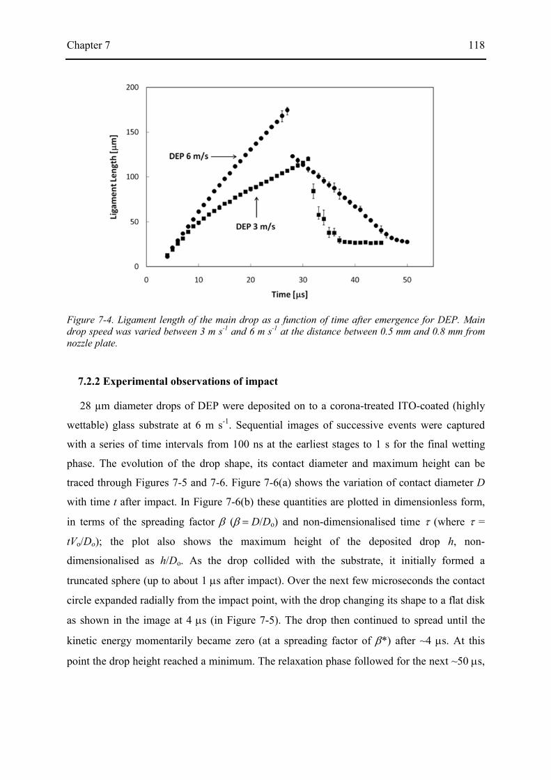
Chapter 7 118
7.2.2 Experimental observations of impact
28 µm diameter drops of DEP were deposited on to a corona-treated ITO-coated (highly
wettable) glass substrate at 6 m s-1. Sequential images of successive events were captured
with a series of time intervals from 100 ns at the earliest stages to 1 s for the final wetting
phase. The evolution of the drop shape, its contact diameter and maximum height can be
traced through Figures 7-5 and 7-6. Figure 7-6(a) shows the variation of contact diameter D
with time t after impact. In Figure 7-6(b) these quantities are plotted in dimensionless form,
in terms of the spreading factor β (β = D/Do) and non-dimensionalised time τ (where τ =
tVo/Do); the plot also shows the maximum height of the deposited drop h, non-
dimensionalised as h/Do. As the drop collided with the substrate, it initially formed a
truncated sphere (up to about 1 µs after impact). Over the next few microseconds the contact
circle expanded radially from the impact point, with the drop changing its shape to a flat disk
as shown in the image at 4 µs (in Figure 7-5). The drop then continued to spread until the
kinetic energy momentarily became zero (at a spreading factor of β*) after ~4 µs. At this
point the drop height reached a minimum. The relaxation phase followed for the next ~50 µs,
Figure 7-4. Ligament length of the main drop as a function of time after emergence for DEP. Main drop speed was varied between 3 m s-1 and 6 m s-1 at the distance between 0.5 mm and 0.8 mm from nozzle plate.
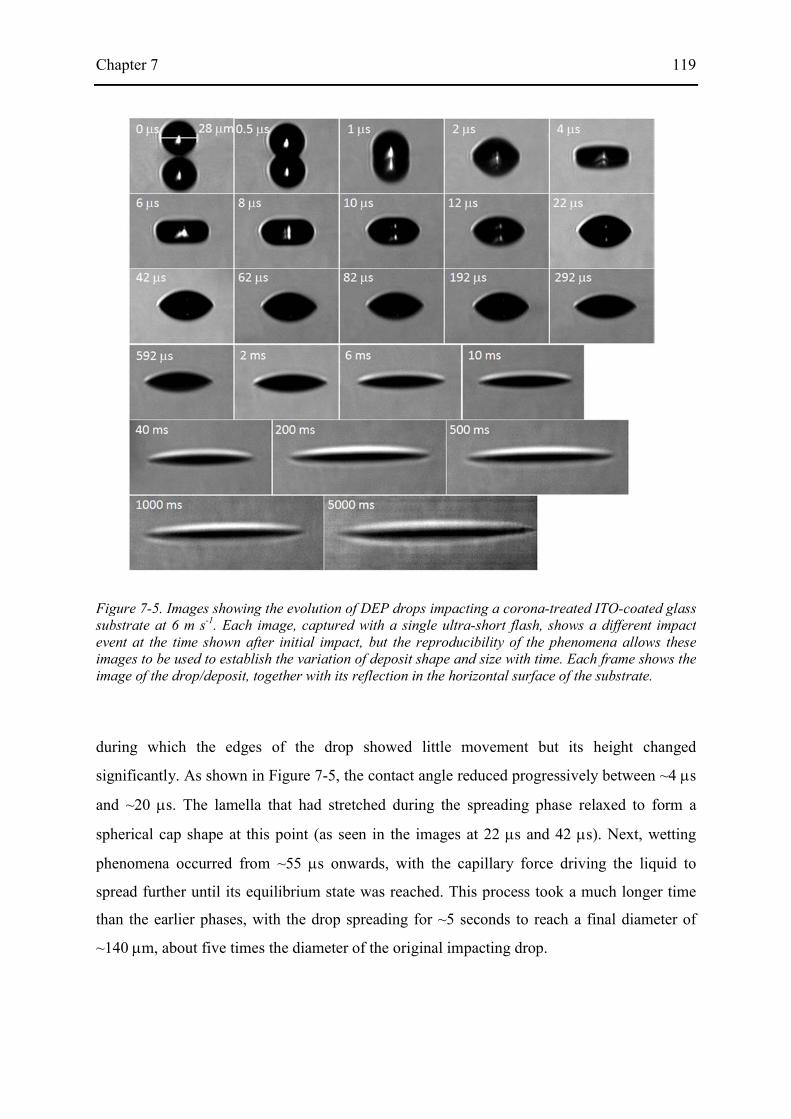
Chapter 7 119
during which the edges of the drop showed little movement but its height changed
significantly. As shown in Figure 7-5, the contact angle reduced progressively between ~4 µs
and ~20 µs. The lamella that had stretched during the spreading phase relaxed to form a
spherical cap shape at this point (as seen in the images at 22 µs and 42 µs). Next, wetting
phenomena occurred from ~55 µs onwards, with the capillary force driving the liquid to
spread further until its equilibrium state was reached. This process took a much longer time
than the earlier phases, with the drop spreading for ~5 seconds to reach a final diameter of
~140 µm, about five times the diameter of the original impacting drop.
Figure 7-5. Images showing the evolution of DEP drops impacting a corona-treated ITO-coated glass substrate at 6 m s-1. Each image, captured with a single ultra-short flash, shows a different impact event at the time shown after initial impact, but the reproducibility of the phenomena allows these images to be used to establish the variation of deposit shape and size with time. Each frame shows the image of the drop/deposit, together with its reflection in the horizontal surface of the substrate.

Chapter 7 120
Figure 7-6. Full history of spreading of DEP drops impacting a corona-treated ITO-coated glass substrate at 6 m s-1 as a function of time. (a) contact diameter D as a function of time t; (b) spreading factor β and dimensionless height h/D0 as a function of dimensionless time τ (=tV0/D0).

Chapter 7 121
Figure 7-7. The effect of impact speed on time evolution of spreading factor β during the kinematic phase for DEP drops impacting a corona-treated ITO-coated glass substrate.
Figure 7-8. The effect of impact speed on time evolution of spreading factor β during the spreading phase for DEP drops impacting a corona-treated ITO-glass substrate.
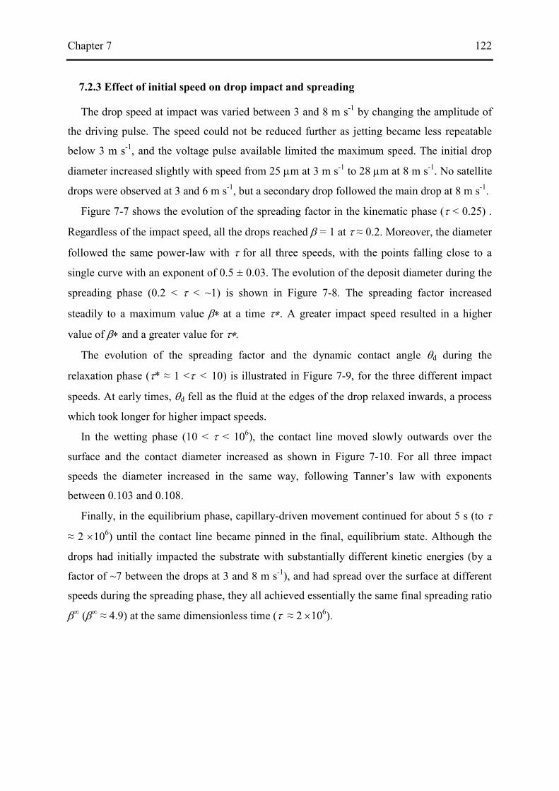
Chapter 7 122
7.2.3 Effect of initial speed on drop impact and spreading
The drop speed at impact was varied between 3 and 8 m s-1 by changing the amplitude of
the driving pulse. The speed could not be reduced further as jetting became less repeatable
below 3 m s-1, and the voltage pulse available limited the maximum speed. The initial drop
diameter increased slightly with speed from 25 µm at 3 m s-1 to 28 µm at 8 m s-1. No satellite
drops were observed at 3 and 6 m s-1, but a secondary drop followed the main drop at 8 m s-1.
Figure 7-7 shows the evolution of the spreading factor in the kinematic phase (τ < 0.25) .
Regardless of the impact speed, all the drops reached β = 1 at τ ≈ 0.2. Moreover, the diameter
followed the same power-law with τ for all three speeds, with the points falling close to a
single curve with an exponent of 0.5 ± 0.03. The evolution of the deposit diameter during the
spreading phase (0.2 < τ < ~1) is shown in Figure 7-8. The spreading factor increased
steadily to a maximum value β∗ at a time τ∗. A greater impact speed resulted in a higher
value of β∗ and a greater value for τ∗.
The evolution of the spreading factor and the dynamic contact angle θd during the
relaxation phase (τ* ≈ 1 <τ < 10) is illustrated in Figure 7-9, for the three different impact
speeds. At early times, θd fell as the fluid at the edges of the drop relaxed inwards, a process
which took longer for higher impact speeds.
In the wetting phase (10 < τ < 106), the contact line moved slowly outwards over the
surface and the contact diameter increased as shown in Figure 7-10. For all three impact
speeds the diameter increased in the same way, following Tanner’s law with exponents
between 0.103 and 0.108.
Finally, in the equilibrium phase, capillary-driven movement continued for about 5 s (to τ
≈ 2 ×10⁶) until the contact line became pinned in the final, equilibrium state. Although the
drops had initially impacted the substrate with substantially different kinetic energies (by a
factor of ~7 between the drops at 3 and 8 m s-1), and had spread over the surface at different
speeds during the spreading phase, they all achieved essentially the same final spreading ratio
β∞ (β∞ ≈ 4.9) at the same dimensionless time (τ ≈ 2 ×10⁶).
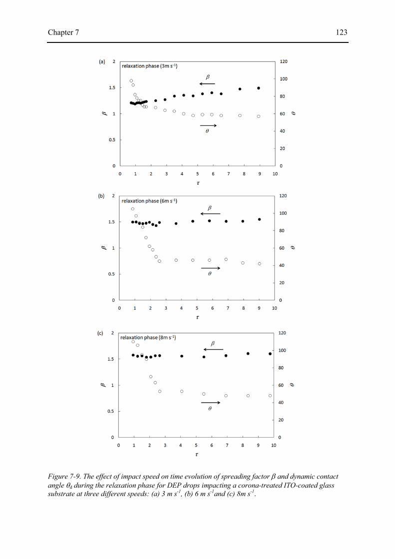
Chapter 7 123
Figure 7-9. The effect of impact speed on time evolution of spreading factor β and dynamic contact angle θd during the relaxation phase for DEP drops impacting a corona-treated ITO-coated glass substrate at three different speeds: (a) 3 m s-1, (b) 6 m s-1and (c) 8m s-1.

Chapter 7 124
7.2.4 Effect of surface wettability on drop impact and spreading
In order to investigate the effect of surface wettability, a series of experiments was
performed with an ITO-coated glass substrate, a corona-treated ITO-coated glass substrate
and a PTFE-coated glass substrate. Except for the treatment of the substrate, all the other
conditions such as drop speed, shape of driving waveform and fluid properties remained the
same. The evolution of the spreading factor for DEP drops at impact speeds of 6 m s-1 on
these three substrates is shown in Figure 7-11. Sequential images of drop evolution for drop
impact on an as-received ITO-glass substrate and PTFE-coated glass substrate are shown
Figure 7-12 and 7-13. The spreading factor increased during the kinematic phase with a
power-law relationship, β ∝ τ0.5 and the durations of the first three phases were the same for
all the substrates.
However, a significant influence of the surface wettability was observed during the
wetting phase. Despite the fact that the drop experienced capillary-driven propagation from
the same value of τ as for the treated ITO-glass substrate, the wetting process on the non-
treated ITO-glass substrate persisted only up to τ ≈ 103. It also deviated from Tanner’s law,
with an exponent of 0.06 ± 0.003. Because of this short wetting time and the lower speed of
movement, β∞ was much smaller (β∞ ≈ 2) than on the more wettable surface. A moderate
change in surface wettability (from θeq = ~4º to θeq = ~32º) resulted in a large difference in
Figure 7-10. The effect of impact speed on time evolution of spreading factor β during the wetting phase for DEP drops impacting a corona-treated ITO-coated glass substrate.

Chapter 7 125
Figure 7-11. Full history of spreading of drops of DEP drops impacting at 6 m s-1 on to corona-treated ITO-coated, as-received ITO-coated and PTFE-coated glass substrates.
Figure 7-12. Images showing the evolution of DEP drops impacting as-received ITO-coated glass substrate at 6 m s-1.

Chapter 7 126
wetting time and in final drop diameter. On the other hand, for impact on a PTFE-coated
substrate no wetting phase was seen and the value of β∞ was smaller than β∗.
7.2.5 Effect of fluid properties on drop impact and spreading
The influences of fluid viscosity and surface tension were investigated by using drops of
two glycerol-water mixtures as well as of DEP, deposited on to a treated-ITO glass substrate
at 6 m s-1. These were chosen to allow a comparison between a pair of fluids with essentially
the same viscosity but different surface tension (DEP and GW 60:40) and a pair with
essentially the same surface tension but different viscosity (GW 60:40 and GW 50:50). The
results are shown in Figure 7-14. The value of surface tension had no effect on the kinematic,
spreading or relaxation phases, but a marked influence on the wetting phase, in terms of the
speed of expansion of the contact diameter and the final spreading factor. In contrast, the
effect of viscosity was negligible throughout the deposition process, with no significant
difference, within the experimental error, between the spreading curves.
Figure 7-13. Images showing the evolution of DEP drops impacting PTFE-coated glass substrate at 6 m s-1.
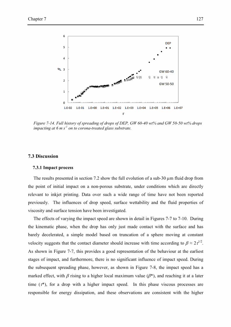
Chapter 7 127
7.3 Discussion
7.3.1 Impact process
The results presented in section 7.2 show the full evolution of a sub-30 µm fluid drop from
the point of initial impact on a non-porous substrate, under conditions which are directly
relevant to inkjet printing. Data over such a wide range of time have not been reported
previously. The influences of drop speed, surface wettability and the fluid properties of
viscosity and surface tension have been investigated.
The effects of varying the impact speed are shown in detail in Figures 7-7 to 7-10. During
the kinematic phase, when the drop has only just made contact with the surface and has
barely decelerated, a simple model based on truncation of a sphere moving at constant
velocity suggests that the contact diameter should increase with time according to β ≈ 2τ1/2.
As shown in Figure 7-7, this provides a good representation of the behaviour at the earliest
stages of impact, and furthermore, there is no significant influence of impact speed. During
the subsequent spreading phase, however, as shown in Figure 7-8, the impact speed has a
marked effect, with β rising to a higher local maximum value (β*), and reaching it at a later
time (τ*), for a drop with a higher impact speed. In this phase viscous processes are
responsible for energy dissipation, and these observations are consistent with the higher
Figure 7-14. Full history of spreading of drops of DEP, GW 60-40 wt% and GW 50-50 wt% drops impacting at 6 m s-1 on to corona-treated glass substrate.
Chapter 7 128
initial kinetic energy of the faster drops. The attainment of the maximum spreading factor
coincides with a minimum height for the drop (as shown in Figure 7-6b). Even though the
initial kinetic energy of the fluid has been dissipated at this point, there is excess surface
energy stored in its non-equilibrium shape, and this drives the subsequent relaxation phase.
As seen in Figure 7-9, there are significant differences with impact speed in the rate and
extent of the changes in drop shape and size during relaxation, but the size at the end of the
relaxation phase varies little with the initial impact speed. Similarly, the wetting behaviour
shown in Figure 7-10 which leads to the final equilibrium deposit at τ > 106 showed no
dependence on the impact speed, being driven by capillary forces.
Figures 7-11 and 7-14 show that changes in the surface energy of the substrate, or the
surface tension of the liquid, had major effects on the wetting phase, but did not make any
detectable difference to the earlier phases. This is in contrast to the observations of Fukai et al.
(1995) who reported that surface wettability affected all phases of the spreading process. In
the present work, as would be expected for capillary-driven flow in the wetting phase, a
lower substrate surface energy led to a smaller final spreading factor (β ∞), which was
reached after a shorter time.
Although it has been reported previously (Kim & Chun 2001) that a large change in fluid
viscosity, within the range from 1 to 100 mPa s, can influence the spreading phase, over the
smaller range of viscosities relevant to ink-jet printing and explored in this work with the two
different glycerol-water mixtures (Figure 7-14), no significant effects of viscosity were
detected in any phase of the impact history.
7.3.2 Prediction of maximum spreading factor
Several comparisons have been reported recently between experimental measurements and
the predictions of spreading factor from analytical or empirical models (van Dam & Clerc,
2004; Dong et al. 2007; Son et al. 2008; Perelaer et al. 2009; Hsiao et al. 2009). However,
there are inconsistencies between the results from some of this work, particularly for the case
of systems with a low contact angle. For example, Perelaer et al. (2009) deposited drops from
a solution of polystyrene in toluene with Re = 110.8 and We = 2.75 on to a glass substrate,
with a static contact angle of <5°. They measured β* ≈ 4.49, compared with a value of 3.75
predicted from the model of Pasandideh-Fard et al. (1996) for these conditions. In contrast,
Dong et al. (2007) deposited drops of a glycerol-water mixture on to a glass substrate under
Chapter 7 129
very similar conditions (with static contact angle ~6°; Re = 100.9; We = 2.77) but reported a
much lower value for β* (~1.7). The reason for this disparity between the values of
β∗ reported by some investigators appears to lie in their definition of β*, as defined in
chapter 2 above. The maximum spreading diameter predicted by models such as that of
Pasandideh-Fard et al. (1996) relates to the value at the end of the initial spreading phase, D*,
and not to the final diameter at the end of wetting, D∞. For the impact of a rapidly-solidifying
drop or for impact on certain partially wettable surfaces, these two quantities may be equal,
but in general they will be different.
Van Dam and Clerc (2004) studied the impact of water drops on to a glass substrate, and
used aqueous silver sols as well as pure water; visual inspection of the printed drops of the
sols after drying allowed them to deduce the maximum deposit diameter. They compared
their results with the predictions from four different models, including that of Pasandideh-
Fard et al. (1996), and found the best agreement with a model based on volume conservation,
which would be expected to predict D∞ rather than D* as discussed above. Son et al. similarly
measured β ∞ for water drops on various surfaces and found a discrepancy between these
values and the values predicted from theoretical models for β∗ (Son et al. 2008).
The results of the present work may help to clarify these disparities. Figure 7-16 shows the
values of β∗ and β ∞ measured for drops of DEP impacting on a treated and a non-treated
ITO-glass substrate at 6 m s-1, compared with the values of β predicted by various models
reviewed in section 2: the models of Collings et al. (1990), Pasandideh-Fard et al. (1996),
Park et al. (2003) and Ukiwe et al. (2005) based on an energy balance and a model based on
volume conservation are shown. The values of β*, at the end of the spreading phase, were
almost the same for all three values of contact angle, but the values of β ∞, measured from
drops at their final equilibrium state, showed a considerable increase with reducing contact
angle. The values of β* are generally well predicted by the energy balance models which all
show little dependence on contact angle in this regime of low Re and We, although there are
small differences between the models. The values of β ∞ are quite accurately predicted by the
volume conservation model.
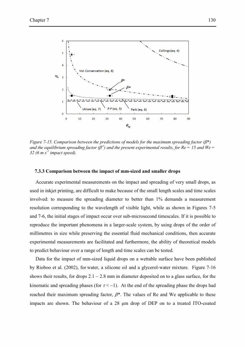
Chapter 7 130
7.3.3 Comparison between the impact of mm-sized and smaller drops
Accurate experimental measurements on the impact and spreading of very small drops, as
used in inkjet printing, are difficult to make because of the small length scales and time scales
involved: to measure the spreading diameter to better than 1% demands a measurement
resolution corresponding to the wavelength of visible light, while as shown in Figures 7-5
and 7-6, the initial stages of impact occur over sub-microsecond timescales. If it is possible to
reproduce the important phenomena in a larger-scale system, by using drops of the order of
millimetres in size while preserving the essential fluid mechanical conditions, then accurate
experimental measurements are facilitated and furthermore, the ability of theoretical models
to predict behaviour over a range of length and time scales can be tested.
Data for the impact of mm-sized liquid drops on a wettable surface have been published
by Rioboo et al. (2002), for water, a silicone oil and a glycerol-water mixture. Figure 7-16
shows their results, for drops 2.1 − 2.8 mm in diameter deposited on to a glass surface, for the
kinematic and spreading phases (for τ < ~1). At the end of the spreading phase the drops had
reached their maximum spreading factor, β*. The values of Re and We applicable to these
impacts are shown. The behaviour of a 28 μm drop of DEP on to a treated ITO-coated
Figure 7-15. Comparison between the predictions of models for the maximum spreading factor (β*) and the equilibrium spreading factor (β∞) and the present experimental results, for Re = 15 and We = 32 (6 m s-1 impact speed).
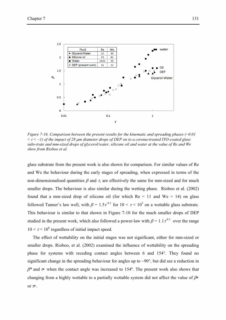
Chapter 7 131
glass substrate from the present work is also shown for comparison. For similar values of Re
and We the behaviour during the early stages of spreading, when expressed in terms of the
non-dimensionalised quantities β and τ, are effectively the same for mm-sized and for much
smaller drops. The behaviour is also similar during the wetting phase. Rioboo et al. (2002)
found that a mm-sized drop of silicone oil (for which Re = 11 and We = 14) on glass
followed Tanner’s law well, with β = 1.5τ 0.1 for 10 < τ < 103 on a wettable glass substrate.
This behaviour is similar to that shown in Figure 7-10 for the much smaller drops of DEP
studied in the present work, which also followed a power-law with β = 1.1τ 0.1 over the range
10 < τ < 106 regardless of initial impact speed.
The effect of wettability on the initial stages was not significant, either for mm-sized or
smaller drops. Rioboo, et al. (2002) examined the influence of wettability on the spreading
phase for systems with receding contact angles between 6 and 154°. They found no
significant change in the spreading behaviour for angles up to ~90°, but did see a reduction in
β* and τ∗ when the contact angle was increased to 154º. The present work also shows that
changing from a highly wettable to a partially wettable system did not affect the value of β∗
or τ∗.
Figure 7-16. Comparison between the present results for the kinematic and spreading phases (~0.01 < t < ~1) of the impact of 28 µm diameter drops of DEP on to a corona-treated ITO-coated glass subs-trate and mm-sized drops of glycerol/water, silicone oil and water at the value of Re and We show from Rioboo et al.
Chapter 7 132
As discussed above, during the kinematic phase the contact diameter of the small DEP
drops was found to increase with a power-law in time, with an exponent of 0.5 ± 0.03 for all
three impact speeds. Rioboo et al. (2002) also reported similar power-law behaviour for their
larger drops, with an exponent lying between 0.45 and 0.57 regardless of impact condition or
surface wettability. During the spreading phase the drops showed differing behaviour,
depending on the values of Re and We. Water, with low viscosity, gave a high Re and
reached the highest value of β*. The spreading data for the small DEP drop and the mm-
sized drops of glycerol–water mixture and silicone oil, which have similar values of Re and
We, are very similar when plotted in terms of the dimensionless variables β and τ, and attain
similar values of β* (1.5 – 1.6).
7.4 Conclusions
The deposition and spreading process of a small drop of Newtonian liquid on to a non-
absorbent smooth surface has been studied, from the initial kinematic phase (τ < ~0.1) to the
long-time equilibrium state (τ > ~106). The conditions were chosen to be representative of
drop-on-demand ink-jet printing, and the work constitutes the first study of drop behaviour at
these values of initial Reynolds and Weber number, with high temporal and spatial resolution,
which extends over eight orders of magnitude in timescale. During the initial kinematic
phase, the contact diameter of the drop followed the power-law relationship expected from a
simple model, β ≈ 2τ 1/2, regardless of impact speed and surface wettability. In the spreading
phase, however, there was significant influence of impact speed, and the time taken to reach
the maximum spreading diameter β∗ increased with speed. At this point the drop had the
shape of a flat disk, which then rapidly recovered in height during the relaxation phase to
form a spherical cap. For the values of Re and We typical of inkjet printing the relaxation was
heavily damped, without the oscillation seen for impacts at higher Re and We. During the
wetting phase (10 < τ < ~106), for a highly wettable surface, the drop then spread outwards,
driven by capillary forces and following Tanner’s law, β ∝ τ 0.1 for all impact speeds.
Measurements of the maximum spreading factor (β∗) were compared with the predictions
of analytical models based on energy balance, which were in reasonable agreement. The
final spreading factor (β∞) showed better agreement with the value predicted from volume

Chapter 7 133
conservation. Some confusion has been identified in the previous literature over the
distinction between these two measures of spreading.
Good correlation was found between the deposition dynamics over the whole range of
timescales of these small drops, and the data for the much larger, mm-sized drops studied in
much previous work, provided that the values of Re and We were similar.

Chapter 8 134
8. Drop impact dynamics: II. Non-Newtonian fluid
8.1 Introduction
The impact and spreading of non-Newtonian fluids on solid surfaces has also played a
key role in many fields of activities such as cooling, painting, food product, tablet coating and
pharmaceutical sprays. Although extensive works on drop impact process of Newtonian
fluids have been done, the mechanism of an inkjet-printed non-Newtonian drop impact on a
wettable surface remains unknown to date.
This chapter aims to answer research question 7 - How do the rheological properties of
viscoelastic ink affect the impact process? We investigate how different the spreading of a
viscoelastic liquid drop on wettable surfaces is from that of a Newtonian liquid drop which
has been studied in the last chapter. Polystyrene solutions in DEP were used in this work, and
the polymer concentration and molecular weight varied to see the effects of increasing
elasticity. The same experimental system and imaging processing techniques as chapter 7
were used here as well.
The experimental results on jetting and deposition behaviour of the polymer solutions are
shown with single-flash images in section 8.2. The effects of polymer molecular weight and
concentration on the jetting and drop impact are discussed in section 8.3.
8.2 Results
8.2.1 Jetting behaviour
The effect on jetting behaviour of adding a very small amount of polymer was investigated.
PS with two different values of molecular weight of 110, 000 g mol-1 (PS 110K) and 210, 000
g mol-1 (PS 210K) was dissolved in DEP to give various concentrations from 0.01 to 0.2 wt%.
The available driving voltage limited the maximum polymer content (0.2% for PS 110K and
0.05% for PS 210K). The voltage amplitude was adjusted in order to achieve a drop speed of
~ 6 m s-1 with actuation duration being fixed at 4 µs in order to compare different fluids with
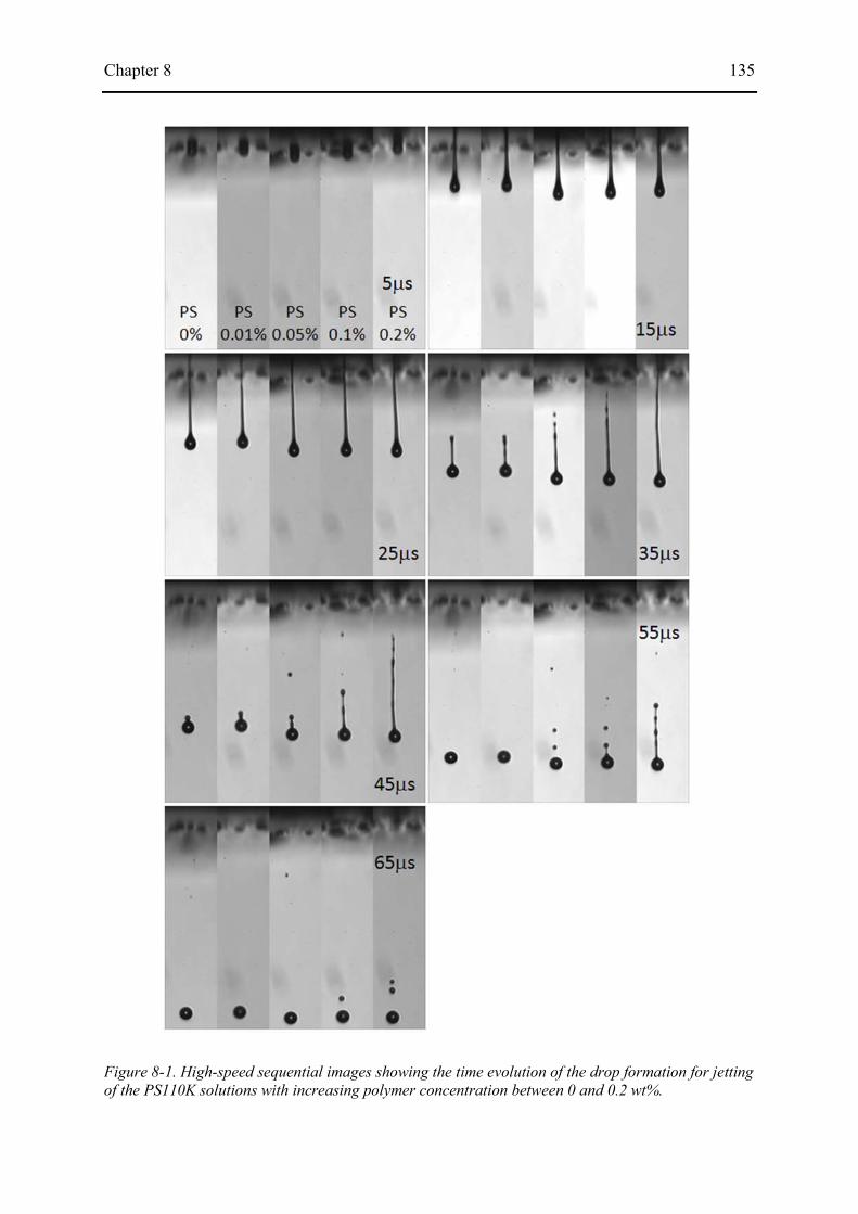
Chapter 8 135
Figure 8-1. High-speed sequential images showing the time evolution of the drop formation for jetting of the PS110K solutions with increasing polymer concentration between 0 and 0.2 wt%.

Chapter 8 136
varying polymer concentration and molecular weight. As seen in chapter 4, there was little
change in shear viscosity (η = ~10 mPa s) and surface tension (σ = 34 mN m-1) with the
polymer additives.
Sequential images of drop formation for the PS 110K solutions with varying polystyrene
concentration are displayed in Figure 8-1. A marked effect of increasing polymer content on
jet formation process is clearly observed. As seen in the images of jets at 5, 15 and 25 µs, all
the solutions exhibited similar behaviour in the stages of initial emergence and jet stretching.
The tip of the jet began to emerge from the nozzle at 4 µs and then formed a primary drop
attached to a thin ligament which stretched until breakup. However, the polymer prevented
Figure 8-2. Instantaneous ligament length plotted against the travel time. (a) PS110K solutions and (b) PS210K solutions with varying concentrations

Chapter 8 137
break-off of the ligament from occurring and induced the formation of a fine filament at the
tail of the ligament. Higher concentration solutions formed longer ligaments than pure DEP
or lower concentration solutions. As observed in the image at 35 µs, a jet of the highest
concentration (PS 110K 0.2%) was still attached to the nozzle. A jet of pure DEP took ~50 µs
for its ligament to collapse into a main drop, while DEP-PS solutions took even longer times
(i.e. ~65 µs for PS 110K 0.2%).
These polymer effects on jetting are more clearly exhibited in a plot of the instantaneous
total ligament length as a function of travel time. As seen in Figure 8-2(a), for all the PS
110K solutions, ligaments were stably extended with stability until break-up. But for the
solutions with higher concentration, rather unstable retraction behaviours were seen with
ligaments splitting into a primary drop and a smaller satellite or two. Increasing polymer
concentration resulted in more elongated ligaments and longer break-up time. Figure 8-2(b)
shows that the higher molecular weight solutions exhibit the same trend but the increase in
ligament length occurred in lower concentration.
Although the ligaments for all the solutions were stretched at the same rate until they
broke up, the subsequent jet shortening speeds were dependent on polymer molecular weight
and concentration. Figure 8-3 shows measured ligament shortening speeds for pure DEP and
the various concentrations of PS 110K and PS 210K solutions and a marked dependence on
Figure 8-3. Ligament shortening speeds measured for pure DEP and various polymer solutions jetted at 6 m/s

Chapter 8 138
the molecular weight and polymer concentration is observed. Initially, we observed that an
overall shortening speed of 4.7 m s-1 for pure DEP. This result is consistent with the constant
jet shortening speed VT (~5 m s-1) that the classical Taylor model predicts given by VT =
2(σ/ρDj)1/2, where Dj is the diameter of a jet ligament (Taylor 1959). The ligaments for the
PS solutions were shortened more rapidly that that for pure DEP. The speed became
higher as the polystyrene concentration increased. The influence of molecular weight is also
clear, with the shortening speed being more sensitive to concentration for higher molecular
weight.
Figure 8-4. Full history of spreading of PS-DEP drops impacting at 6 m s-1 on a corona-treated ITO-coated substrate. (a) PS 110K solutions with varying concentration from 0.01% to 0.2%; (b) 0.05% PS solutions with varying molecular weight from 110K to 488K, as well as pure DEP for comparison

Chapter 8 139
8.2.2 Deposition behaviour
The influences of viscoelasticity were investigated by using drops of various PS solutions,
deposited at 6 m s-1on to a highly wettable corona-treated ITO-glass substrate. The time
evolution of the drop diameters for the PS 110K solutions with varying concentrations (0.01%
< c < 0.2%) are plotted in Figure 8-4(a). The presence of viscoelasticity due to increasing
polymer concentration had no effect on any stage of drop impact. As shown in this graph, all
the measurements of contact diameter with time showed essentially the same trend as the
progression of a pure DEP drop (shown in Figure 8-4(b)) for all the concentrations. The
scatter of the data in the kinematic phase was caused by the slight deterioration of jetting
repeatability of the polymer solutions in the retraction process as seen in section 8.2.1.
Typical sequential images of the impact process for the PS 110K 0.2% solutions are seen in
Figure 8-5.
The effect of molecular weight (110,000 g mol-1 < Mw < 488,000 g mol-1) was also
examined while fixing the polymer concentration at 0.05%. As represented in Figure 8-4(b),
the influence of molecular weight was also negligible throughout the whole deposition
process, with no significant difference, within the experimental error, between the spreading
curves.
Figure 8-5. Single-flash images showing the evolution of drop impact of 0.2% DEP-PS 110K solution at 6 m/s on a treated ITO-coated glass substrate
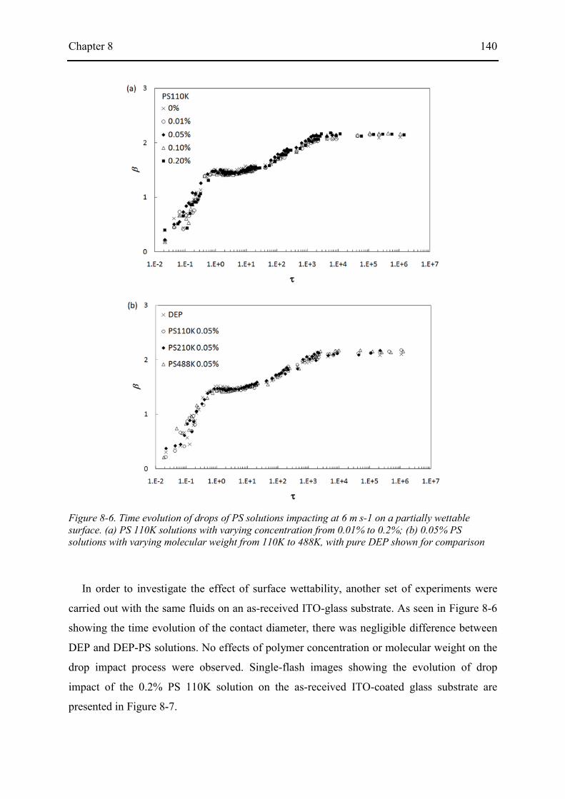
Chapter 8 140
In order to investigate the effect of surface wettability, another set of experiments were
carried out with the same fluids on an as-received ITO-glass substrate. As seen in Figure 8-6
showing the time evolution of the contact diameter, there was negligible difference between
DEP and DEP-PS solutions. No effects of polymer concentration or molecular weight on the
drop impact process were observed. Single-flash images showing the evolution of drop
impact of the 0.2% PS 110K solution on the as-received ITO-coated glass substrate are
presented in Figure 8-7.
Figure 8-6. Time evolution of drops of PS solutions impacting at 6 m s-1 on a partially wettable surface. (a) PS 110K solutions with varying concentration from 0.01% to 0.2%; (b) 0.05% PS solutions with varying molecular weight from 110K to 488K, with pure DEP shown for comparison

Chapter 8 141
8.3 Discussion
8.3.1 Effect of polymer on jetting
The small addition of polymer investigated here has a significant effect on jetting in terms
of ligament elongation and retraction. The effect of elasticity induced by a very small amount
of polymer addition cannot be negligible, and can even govern the process of ligament
formation. This observation cannot be explained by the low shear viscosities of the
viscoelastic fluids which do not vary over these polymer concentrations.
This influence of elasticity on jet formation and evolution can be identified with the help
of high frequency rheometry. As discussed in Chapter 4, fluid properties measured by shear
rate viscometers do not effectively distinguish between solutions having different degree of
elasticity. But, good correlation was found between the degree of elasticity of the polymer
solution and the maximum ligament length. The elasticity ratio G′/|G*| was obtained from
PAV rheometry to quantify the degree of elasticity. Figure 8-8 compares this ratio with MLL
as a function of polymer concentration for the PS 110K and PS 210K solutions. It is obvious
that there is a strong correlation between the maximum ligament length and the elasticity. All
of the solutions show an increase in the maximum ligament length as the elasticity modulus
(G′) increased, suggesting that stretching and shortening of the ligament is controlled by the
extent of the fluid’s elasticity.
Figure 8-7. Single-flash images showing the evolution of drop impact of 0.2% DEP-PS 110K solution at 6 m/s on an ITO-coated glass substrate
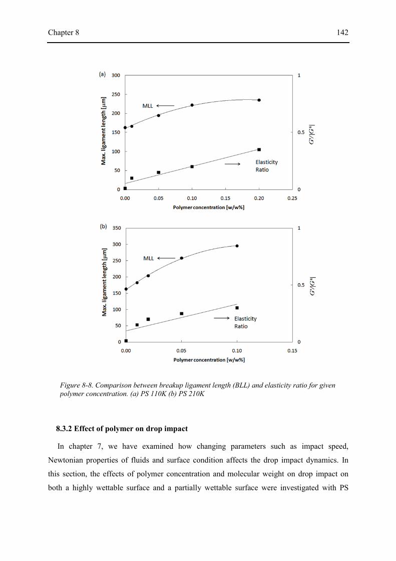
Chapter 8 142
8.3.2 Effect of polymer on drop impact
In chapter 7, we have examined how changing parameters such as impact speed,
Newtonian properties of fluids and surface condition affects the drop impact dynamics. In
this section, the effects of polymer concentration and molecular weight on drop impact on
both a highly wettable surface and a partially wettable surface were investigated with PS
Figure 8-8. Comparison between breakup ligament length (BLL) and elasticity ratio for given polymer concentration. (a) PS 110K (b) PS 210K
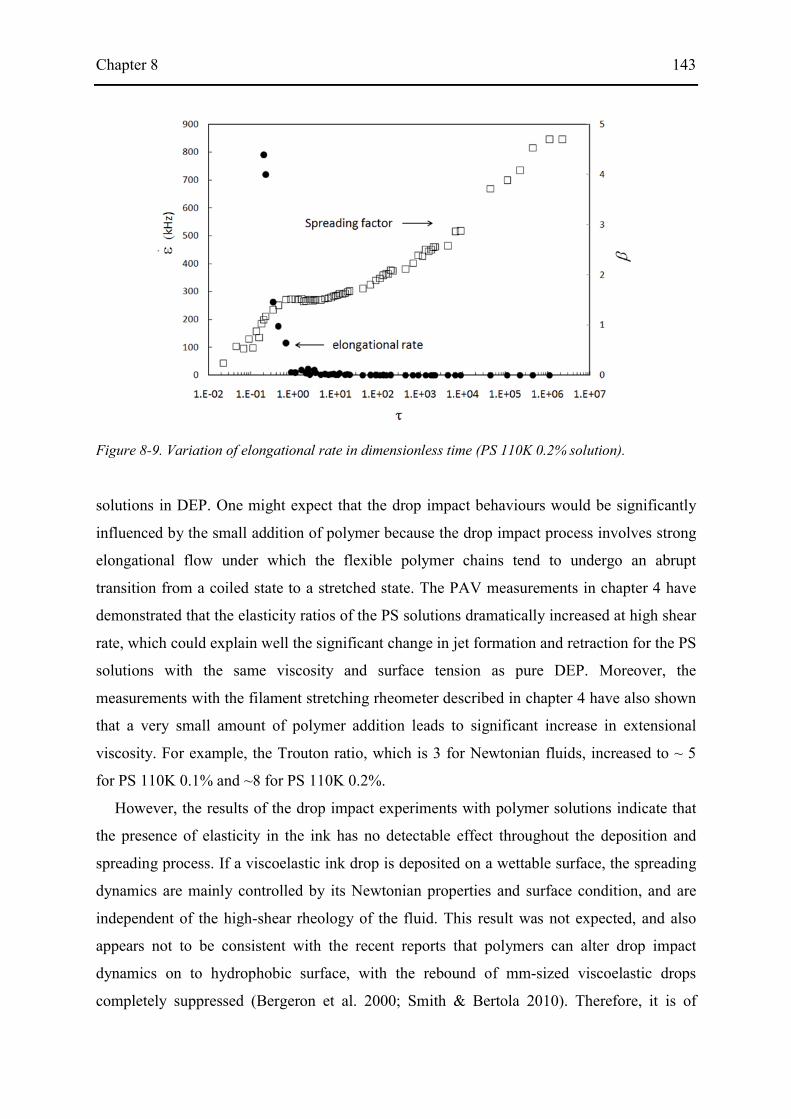
Chapter 8 143
solutions in DEP. One might expect that the drop impact behaviours would be significantly
influenced by the small addition of polymer because the drop impact process involves strong
elongational flow under which the flexible polymer chains tend to undergo an abrupt
transition from a coiled state to a stretched state. The PAV measurements in chapter 4 have
demonstrated that the elasticity ratios of the PS solutions dramatically increased at high shear
rate, which could explain well the significant change in jet formation and retraction for the PS
solutions with the same viscosity and surface tension as pure DEP. Moreover, the
measurements with the filament stretching rheometer described in chapter 4 have also shown
that a very small amount of polymer addition leads to significant increase in extensional
viscosity. For example, the Trouton ratio, which is 3 for Newtonian fluids, increased to ~ 5
for PS 110K 0.1% and ~8 for PS 110K 0.2%.
However, the results of the drop impact experiments with polymer solutions indicate that
the presence of elasticity in the ink has no detectable effect throughout the deposition and
spreading process. If a viscoelastic ink drop is deposited on a wettable surface, the spreading
dynamics are mainly controlled by its Newtonian properties and surface condition, and are
independent of the high-shear rheology of the fluid. This result was not expected, and also
appears not to be consistent with the recent reports that polymers can alter drop impact
dynamics on to hydrophobic surface, with the rebound of mm-sized viscoelastic drops
completely suppressed (Bergeron et al. 2000; Smith & Bertola 2010). Therefore, it is of
Figure 8-9. Variation of elongational rate in dimensionless time (PS 110K 0.2% solution).
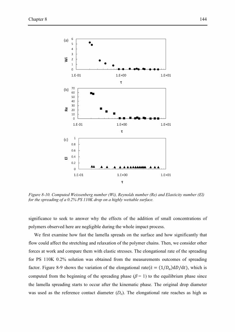
Chapter 8 144
significance to seek to answer why the effects of the addition of small concentrations of
polymers observed here are negligible during the whole impact process.
We first examine how fast the lamella spreads on the surface and how significantly that
flow could affect the stretching and relaxation of the polymer chains. Then, we consider other
forces at work and compare them with elastic stresses. The elongational rate of the spreading
for PS 110K 0.2% solution was obtained from the measurements outcomes of spreading
factor. Figure 8-9 shows the variation of the elongational rate(ε� = (1/��)d�/d�), which is
computed from the beginning of the spreading phase (β = 1) to the equilibrium phase since
the lamella spreading starts to occur after the kinematic phase. The original drop diameter
was used as the reference contact diameter (Do). The elongational rate reaches as high as
Figure 8-10. Computed Weissenberg number (Wi), Reynolds number (Re) and Elasticity number (El) for the spreading of a 0.2% PS 110K drop on a highly wettable surface.

Chapter 8 145
~800 kHz at the beginning of the spreading phase and rapidly falls until the drop reaches the
relaxation phase. It ends up close to zero during the wetting phase because of the very slow
speed of capillary wetting.
The Weissenberg number (Wi = τ ��) is then computed for the characteristic relaxation
time of PS 110K polymer in elongational flow. As mentioned in chapter 3, the molecular
transition from coil to stretched state tends to occur at a critical Weissenberg number, Wi =
0.5. For this ultra dilute solution the molecular relaxation-controlled unravelling time is
effectively the same as the Zimm relaxation time of the polymer (λz = 6.7 µs for PS 110K),
and linearly increases from c/c* = 0.1 (Clasen et al. 2006). Figure 8-10(a) shows the value of
Wi for the spreading and relaxation phase as well as the Reynolds number for the flow. They
exhibit the same trend with time because Wi number is a function of the elongational rate. At
the beginning of the spreading phase Wi is more than 5 and quickly decreases as the
elongation rate reduces.
Polymers in solution do not influence the spreading dynamics at all during the wetting
phase because of the very slow spreading rate (ε� ~ 0). Because the velocity gradient is not
large enough to stretch the polymer, the polymer molecule behaves like a spherical particle
advected by the bulk flow. As seen from the PAV measurements in chapter 4, these dilute
polymer solutions do not exhibit elastic behaviour at low frequency (f < ~1 kHz) even in the
inertialess, oscillatory shear flow. Therefore, at this slow elongational rate relevant to wetting
the molecular friction as well as viscous dissipation are not increased.
However, the high Weissenberg number for the initial spreading phase suggests that in the
phase all the polymer chains may be stretched and interact with each other, which should
affect the spreading dynamics. Nevertheless, no polymer effects were detected over the whole
deposition process. There are two possible reasons why no significant differences are
observed between the viscoelastic PS solutions and Newtonian DEP in terms of impact
dynamics, even though they are under highly extensional flow.
First, for a polymer molecule to be fully stretched, the time for which Wi > 0.5 is required
to persist for at least order of the Zimm relaxation time. Thus, although the elongational flow
during the drop spreading may be strong enough to cause Wi exceeds 0.5, it rapidly decays
within ~3 µs (τ ≈ 0.7), which is shorter than the longest relaxation time of PS 110K polymer
(λz = 6.7 µs). Therefore, it is not likely that the PS110K polymer chains become fully
stretched in this short time scale.

Chapter 8 146
Second, although the fluid properties play important roles in the drop deposition process,
there are other forces at work that need to be taken into account. Because inertial force is
dominant in the spreading and relaxation phases, it is necessary to consider the relative
importance of elastic stress to inertial force. To do it, we calculated Reynolds number using
the contact diameter as a characteristic length for these phases, and obtain the variation of
Elasticity number (El = Wi/Re), the ratio between inertial force and elastic stress. As seen in
Figure 8-10(b) and (c), Re has high values at high Wi, which results in very low values of El
(<0.1) throughout the whole duration of impact. We infer from this that in the initial stage of
impact the elastic stress cannot compete with the overwhelming inertial force and is
completely negligible.
Figure 8-11. Computed Weissenberg number (Wi), Reynolds number (Re) and Elasticity number (El) for the spreading of a 0.05% PS 480K drop on a highly wettable surface.

Chapter 8 147
The PS 488K polymer has a far longer Zimm relaxation time (λZ = 85.6 µs) than PS110K
which leads to a larger Wi than that for PS110K. Figure 8-11(a) shows the computed Wi for
the 0.05% PS 488K solution, together with the calculated value of Re and El. The fact that El
reaches ~1 initially and decreases to ~ 0.6 from τ = 1 hints that elastic stress for this solution
may compete with inertial force. However, as mentioned above, the time for which Wi > 0.5
was only ~3 µs (τ ≈ 0.7), and Wi number then rapidly reduced almost to zero. Therefore, the
effect of the viscoelasticity in this fluid system was also negligible throughout the deposition
process.
8.4 Conclusions
We seek to understand the role of rheology on drop impact and spreading over the
timescale and lengthscale encountered in inkjet printing. The deposition process for an inkjet-
printed viscoelastic drop on to a wettable surface has been studied over eight orders of
magnitude in timescale. The addition of a small concentration of polystyrene in DEP resulted
in a longer break-up ligament length and a faster retraction speed in flight. However, the
presence of viscoelasticity had no effects on any stage of drop impact on a wettable surface.
Although in the spreading phase the extensional rate was strong enough to stretch the
polymer chains (maximum Wi number > 5), elastic stresses were still negligible for two
reasons: (1) the extensional flow was momentarily very strong in the beginning of the
spreading phase, but the high rate persisted for a much shorter time than the Zimm relaxation
time of the polymer; and (2) Elasticity number < 1 suggested that inertia force dominated the
phase and elasticity stresses could not overwhelm it. For the relaxation and wetting phase,
because the lamella experienced very slow spreading, non-Newtonian fluids showed the same
behaviour as Newtonian fluids. It can therefore be concluded that, even for viscoelastic inks,
the deposition process is mainly controlled by their Newtonian properties and the surface
condition, and is independent of the high-shear rate rheology of the fluid.
Chapter 9 148
9. Summary and overall discussion
This thesis has sought to enhance our understanding of drop impact process in the context
of industrial inkjet printing. It has been divided into three major research topics. First, it was
essential to gain background knowledge in ink rheology and to acquire technical skills for
measuring and analysing the rheological properties of viscoelastic fluids. The collision of two
liquid jets was explored as a method of subjecting the liquid to extensional flow.
Unexpectedly having found the fishbone regime corresponding to lower Reynolds and Weber
numbers than had been previously reported, we explored the possibility that the information
about the printability of a polymer-containing fluid could be obtained, without using a
printhead, by observing the remarkably symmetrical fishbone structure which was produced
by the oblique collision of two liquid jets.
Second, it was critical to build an optical imaging system which was capable of imaging
deposited drops at various impact stages, from initial contact to wetting. No experimental
work in the past has attempted to investigate the impact dynamics of an inkjet-printed drop
over such a wide range of time scale. However, our fully automated high-speed imaging
system based on flash-photography has made it possible to acquire clear images of fast
spreading drops for up to 10 s with a time resolution of 100 ns.
Third, the optical system developed in this work has enabled us to study the full history of
the impact dynamics of sub-30 µm drops on various substrates. Particularly, it has been
demonstrated for the first time how an inkjet-printed drop collides, spreads, relaxes and wets
on a highly wettable surface over eight orders of magnitude in timescale. We have
investigated how changing parameters such as impact condition, Newtonian and non-
Newtonian fluid properties and surface condition affect drop deposition behaviour at different
phases.
The main findings of this thesis and the corresponding answers of the research questions
are summarized as follows:
Research question 1: Which techniques can be used to assess the rheological properties
of various functional polymer inks in the context of inkjet printing?
Chapter 9 149
The understanding and control of jet formation and subsequent drop deposition
mechanisms for viscoelastic ink require physical studies into liquid properties at very
high shear rates, stretching of fluid ligaments, the role of polymers in drop spreading and
wetting. Conventional viscometers and rheometers cannot clearly distinguish between
rheological properties of low viscoelastic polymer fluids whose elastic effects appear
only at high frequency. Linear viscoelastic moduli (G′and G′′) can be determined by
piezo-axial vibrator (PAV) as a function of frequency. The PAV measurements for
polystyrene (PS) solutions demonstrate that there is a strong increase in elasticity with
polymer concentration and with shear rate (frequency). The viscoelastic effect of the
polymer solutions in extensional flow, which is crucial in the inkjet printing process, can
be measured by using a filament stretching rheometer. A high speed camera captures the
motion of the fluid which is initially placed between two circular pistons and then
stretched to a fixed distance. For example, the maximum extensional viscosity of the PS
solutions is greater than that of pure DEP. The Trouton ratio grows dramatically with the
small addition of polymer in the Newtonian solvent.
Research question 2: Is there any new simple method to assess the printability of non-
Newtonian inkjet fluids, without using an inkjet print head?
There have been attempts to evaluate jetting performance of an inkjet print head
without involving the inkjet printer itself. High frequency rheometry methods such as
piezoelectric axial vibration and the filament-stretching rheometer have proved to be
useful. However, these methods require a strong background in rheology and specialised
skills for the measurement, and are not widely available. The work described here is
suggests that the printability of a viscoelastic fluid can be assessed by observation of the
"fishbone" structure produced by the oblique collision of two liquid jets of the fluid. This
symmetrical fluid pattern does not occur for completely symmetrical jet collision: some
asymmetry is essential. We introduce various ways to achieve the asymmetry: by the use
of different lengths of free jet, by displacing the jets laterally, or by disturbing the surface
of one jet. It has also been discovered that elasticity has a strong effect on the formation
and fragmentation of the fluid sheet formed by the oblique collision of the jets. Good
correlation is found between the maximum fishbone angle and the maximum ligament
length measured in jetting experiments from a DoD print head, which suggests that the
Chapter 9 150
fishbone phenomenon may provide a simple and useful tool to explore the upper limit of
polymer concentration in ink jet printing fluids.
Research question 3: What is the best optical system to acquire high quality images of
sub-30 µm drops over a wide range of time scale and which image processing technique
can be applied to extract relevant information from the obtained images?
Development of full understanding of the drop impact dynamics on a solid surface is
critically dependent on how clear images of a deformed drop can be obtained as it
impacts and spreads on the surface. Cinematography involving a high-speed camera has
its limitations in recording speed. Commercially available high-speed cameras cannot be
utilized to image a sub-30 µm drop because of their limited recording speed. Short-
duration flash photography was used to observe the various stages, with images captured
over a range of timescales from every 100 ns during the rapidly developing early stages
(equivalent to 10 million frames per second) to every second for the final stage.
A simple thresholding technique to detect edges of a drop could not be applied because
the total intensity of light emitted by the spark flash varied from image to image. A
advanced edge detection method was therefore adopted to extract quantitative
information from the image. This technique proved to be highly tolerant of varying
background level of captured images.
Research question 4: What are the key parameters of a Newtonian ink affecting drop
spreading and wetting behaviour?
The influences of fluid viscosity and surface tension were investigated by using drops
of two glycerol-water mixtures as well as of DEP, deposited on to a treated-ITO glass
substrate at 6 m s-1. The value of surface tension had no effect on the kinematic,
spreading or relaxation phases, but a marked influence on the wetting phase, in terms of
the speed of expansion of the contact diameter and the final spreading factor. In contrast,
the effect of viscosity was negligible throughout the deposition process, with no
significant difference between spreading curves.
The drop speed at impact was also varied between 3 and 8 m s-1 in order to examine its
effect on drop motion and the final equilibrium diameter. During the kinematic phase
there is no significant influence of impact speed. During the subsequent spreading phase,
however, a greater impact speed resulted in a higher value of β* and a greater value for
Chapter 9 151
τ*. There are significant differences with impact speed in the rate and extent of the
changes in drop shape and size during the relaxation phase, but the size at the end of the
relaxation phase varies little with the initial impact speed. The wetting phase driven by
capillary forces, and the final equilibrium deposit did not show any dependence on the
impact speed. Therefore, it is concluded that surface tension of the ink and the wettability
of the surface play a key role in determining the drop’s final diameter, and the final drop
diameter can be controlled by carefully selecting the surface tension of an ink.
Research question 5: How can those parameters contribute to theoretical models for
the whole process of drop impact?
During the kinematic phase, when the drop has only just made contact with surface and
has barely decelerated, a simple model based on truncation of a sphere moving at
constant velocity suggests that the contact diameter should increase with time according
to β≈2τ1/2. The measurement results in chapter 7 provided a good representation of the
behaviour at the earliest stages of impact, and there were no significant influences of
impact speed, viscoelasticity and surface tension.
Models derived from energy conservation have been used to predict the maximum
spreading diameter. Although these models involved Re, We and θeq, we have shown that
the maximum spreading factor was not significantly dependent on any of those terms, at
least for the fluids and substrates used in this work. The results in Chapter 7 helped to
clarify the disparities between the experimental measurements from previous papers. The
final deposit diameter was quite accurately predicted by the volume conservation
equation.
Tanner’s law that the contact diameter increases slowly with time according to a power
law was found to be valid for the impact of low-surface tension drops on to a highly
wettable surface. The value of the index n was found to be ~0.1 both on theoretical
grounds and from experiments conducted with both mm-sized and µm-sized drops. But,
when either the fluid had high surface tension or the surface was not highly wettable, the
wetting process did not proceed well and the power law index was no longer ~0.1.
Research question 6: How does the drop impact process vary with different substrate
surface conditions?

Chapter 9 152
A series of experiments was performed with an ITO-coated glass substrate, a corona-
treated ITO-coated glass substrate and a PTFE-coated glass substrate. Changes in the
surface energy of the substrate, or the surface tension of the liquid, had major effects on
the wetting phase, but did not make any detectable difference to the earlier phases. A
moderate change in surface wettability from θeq = ∼4° to θeq = ∼32° resulted in a large
difference in wetting time and in final drop diameter. On the other hand, for impact on a
PTFE-coated substrate no wetting phase was seen and the value of β∞ was smaller than
β *.
Research question 7: How do the rheological properties of viscoelastic ink affect the
impact and spreading process?
It has been demonstrated that the addition of a small concentration of polystyrene in
DEP resulted in longer break-up ligament length and faster ligament retraction speed in
flight. Thus, we expected that the drop impact process, particularly the initial phases with
highly extensional flow, would have been significantly influenced by the presence of
viscoelasticity induced by the polymer. However, contrary to our expectation, the
increased viscoelasticity had no effect on any stage of drop impact on a wettable surface.
Although the degree of extension rate in the kinematic and spreading phases was
sufficient to stretch the polymer chains, the high extensional flow did not persist longer
than the Zimm relaxation time of the polymer. In addition, inertial forces dominated
those phases and the elastic stresses induced by polymer chain-to-chain interactions were
negligible in comparison.
Further work
Figure 9-1 Overall inkjet printing process to fabricate organic semiconductor electronics.
This thesis has focused on how fluid properties change with the small addition of polymer
additives and the changed fluid properties affect inkjet performances in both jetting and
Ink formulation
Fluid properties
Inkjet performances
Device performances
Manufactur-ability

Chapter 9 153
deposition on a substrate. As seen in Figure 9-1, the next step to move is to study the
correlation between inkjet performances and device performances, which have not been
understood yet. Here are some possible research topics
1. Inkjet-printed line morphologies
There is further interest on studying the physics of post-impact process (e.g. drying)
which is of great importance in the manufacture of organic semiconductor devices,
with fluid flow and solute (or particle) distribution (Derby 2010). Further studies of
drop coalescence and inkjet-printed line morphologies are necessary for the fabrication
of integrated circuits. Ideal printed lines would be smooth, even and straight, but
recent work has shown that there is a need to improve the control of the behaviour of
line formation of functional inks (Soltman & Subramanian 2008). There has been little
effort, so far, to investigate how rheological properties of polymer inks or functional
inks containing nano-particles such as silver, carbon nanotubes or graphene influence
the performances of electronic devices fabricated by inkjet printing process.
2. Inkjet printing on a patterned substrate
This thesis has studied a single drop impact on a flat substrate, and it would be of
significance to continue to study the drop impact process on a patterned substrate. Few
attentions has been paid to interaction between inkjet-printed polymer materials and
the patterned substrate for the application of OLED displays; how they spread, how
they fill out a pixel well, how they dry to form a film, with different kinds of substrates
and fluids. This study would assist the development of a more robust printing process
leading to better quality OLEDs.
3. Optimisation of P3HT:PCBM blend solution for solar cells
As reviewed in chapter 2, there have been efforts to fabricate solar cells with using
inkjet printers. Although various studies investigate the influence of molecular weight
distribution of P3HT on charge carrier mobility and device performance for spin-
coated film (Hoth 2009), little work has done on how changing the polymer blend
formulation (therefore, changing its fluid properties) affects inkjet-printed film and
hence solar cell performances.
4. Top-gate test TFTs on plastic substrate with inkjet-printed active layer island
Many solution-processed organic semiconductor materials have been demonstrated to
exhibit field-effect mobilities on the order of 0.1–1 cm2V-1s-1. As reviewed in chapter
2, a large number of research groups have used inkjet printing technology to fabricate

Chapter 9 154
organic thin film semiconductors. However, little effort has been made to date in
understanding how concentration or molecular weight of N-type and P-type
semiconducting polymers including Polyera N2200 (P(NDI2OD-T2)) and poly(2,5-
bis(3-tetradecylthiophene-2-yl)thieno[3,2-b]thiophene) (pBTTT) influence inkjet
printing process (both jetting and deposition) and hence semiconductor performance
such as mobility, reliability and characteristic curve. Particularly, it would be
interesting to study drop deposition process of those materials on plastic substrates.
Given the remarkable recent progress of inkjet printing to new areas of polymer deposition,
a bright and strong future is anticipated for this technology in the printed electronics field.
Full exploitation of the potential of inkjet printing technology as a non-contact, precise
patterning tool for fabricating organic semiconductor electronics will require further research
into all these aspects.

155
Appendix
Drop deposition system programmed by Labview (National Instruments)
Physical channel parameters
- Camera: image input from camera
- Physical channel: two analogue output ports (one for the delayer and the other for the
print head via the waveform amplifier)
- Lines: trigger line to the motion stage
Setting image file path and name
- Path: File path to save acquiring images
- File name: pre-designated file name for the images. The value of delay time at the
moment of image acquisition will be automatically added when each image is saved.
- Turn on the green light to save the images

156
Controlling the delay unit (DF535)
- Each delay port of the delay unit (A to D) can be set separately by inserting number in
the boxes
- In order to take continuous pictures at different times, the user can generate a list of
delay times in excel format and the programme will upload the file to read.
- Turn on the green light to use the excel file
Waveform generation
- Enter time duration (Tick) in microsecond and voltage amplitude (-10 to 10V)
- By setting multiple points, the user can make any type of waveform
Set and monitor timing parameters
- Loop time (ms): the time to complete one run of the programme (e.g. from waveform
generation to acquire an image). The user can determine jetting frequency by changing
this value (e.g. 200ms 5 Hz)
- Current delay: current delay time is shown here
- Current #: the current number of jetting is shown here
Waveform graph
- The shape of the waveform which the user have made in is shown in this graph
Image display
- Each acquired image is displayed here in real time
Programme starts
Programme stop
157
References
A-Alamry, Khalid, Keith Nixon, Rachel Hindley, Jeffrey A. Odel, and Stephen G. Yeates. “Flow-Induced Polymer Degradation During Ink-Jet Printing.” Macromolecular Rapid Communications 31 (November 2010): 316-320.
Aernouts, T., T. Aleksandrov, C. Girotto, J. Genoe, and J. Poortmans. “Polymer based organic solar cells using ink-jet printed active layers.” Applied Physics Letters 92, no. 3 (2008): 033306.
Anna, Shelley L., and Gareth H. McKinley. “Elasto-capillary thinning and breakup of model elastic liquids.” Journal of Rheology 45, no. 1 (2001): 115.
Attané, P., F. Girard, and V. Morin. “An energy balance approach of the dynamics of drop impact on a solid surface.” Physics of Fluids 19, no. 1 (2007): 012101.
Baeg, Kang-Jun, Dongyoon Khim, Dong-Yu Kim, Soon-Won Jung, Jae Bon Koo, In-Kyu You, Henry Yan, Antonio Facchetti, and Yong-Young Noh. “High speeds complementary integrated circuits fabricated with all-printed polymeric semiconductors.” Journal of Polymer Science Part B: Polymer Physics 49, no. 1 (January 2011): 62-67.
Bartolo, Denis, Arezki Boudaoud, Grégoire Narcy, and Daniel Bonn. “Dynamics of Non-Newtonian Droplets.” Physical Review Letters 99, no. 17 (October 2007): 174502.
Battal, Turgut, C.D. Bain, and R.C. Darton. “Surfactant adsorption and Marangoni flow in liquid jets:: I. Experiments.” Journal of colloid and interface science 263, no. 1 (2003): 250–260.
Bazilevskii, A. V., J. D. Meyer, and A. N. Rozhkov. “Dynamics and Breakup of Pulse Microjets of Polymeric Liquids.” Fluid Dynamics 38, no. 4 (May 2005): 468-392.
Beeson, Rob. “THERMAL ( TIJ ) OR PIEZO ?, WHO CARES ?” IMI 7th ANNUAL INK JET PRINTING CONFERENCE (1998).
Bennett, T., and D. Poulikakos. “Splat-quench solidification: estimating the maximum spreading of a droplet impacting a solid surface.” Journal of Materials Science 28, no. 4 (1993): 963-970.
Bergeron, V, D Bonn, Jy Martin, and L Vovelle. “Controlling droplet deposition with polymer additives.” Nature 405, no. 6788 (June 2000): 772-5.
Bharathan, Jayesh, and Yang Yang. “Polymer electroluminescent devices processed by inkjet printing: I. Polymer light-emitting logo.” Applied Physics Letters 72, no. 21 (1998): 2660.
Bohlin-Instruments. A basic introduction to rheology. Bohlin Instruments Ltd, 1994.
158
Bonn, Daniel, Jens Eggers, Joseph Indekeu, Jacques Meunier, and Etienne Rolley. “Wetting and spreading.” Reviews of Modern Physics 81, no. 2 (May 2009): 739-805.
Bossard, Frédéric, Nadia El Kissi, Alessandra D’Aprea, Fannie Alloin, Jean-Yves Sanchez, and Alain Dufresne. “Influence of dispersion procedure on rheological properties of aqueous solutions of high molecular weight PEO.” Rheologica Acta 49, no. 5 (December 2009): 529-540Bremond, N., C. Clanet, and Emmanuel Villermaux. “Atomization of undulating liquid sheets.” Journal of Fluid Mechanics 585 (August 2007): 421.
Bremond, N., and Emmanuel Villermaux. “Atomization by jet impact.” Journal of Fluid Mechanics 549, no. -1 (February 2006): 273.
Brunahl, J. “Piezoelectric shear mode drop-on-demand inkjet actuator.” Sensors and Actuators A: Physical 101, no. 3 (October 2002): 371-382.
Burroughes, Jh, Ddc Bradley, Ar Brown, Rn Marks, K. Mackay, Rh Friend, Pl Burns, and Ab Holmes. “Light-emitting diodes based on conjugated polymers.” Nature 347, no. 6293 (1990): 539–541.
Bush, J.W.M., and Ae Hasha. “On the collision of laminar jets: fluid chains and fishbones.” Journal of Fluid Mechanics 511 (2004): 285-310.
Caironi, Mario, Enrico Gili, Tomo Sakanoue, Xiaoyang Cheng, and Henning Sirringhaus. “High yield, single droplet electrode arrays for nanoscale printed electronics.” ACS nano 4, no. 3 (March 2010): 1451-6.
Cambridge Display Technology. “Recent Advances in Polymer OLED Technology.” www.cdtltd.co.uk, current press release (2007).
Chandra, Sanjeev, and C. T. Avedisian. “On the Collision of a Droplet with a Solid Surface.” Proceedings of the Royal Society A: Mathematical, Physical and Engineering Sciences 432, no. 1884 (January 1991): 13-41.
Chen, Li-Min, Ziruo Hong, Gang Li, and Yang Yang. “Recent Progress in Polymer Solar Cells: Manipulation of Polymer:Fullerene Morphology and the Formation of Efficient Inverted Polymer Solar Cells.” Advanced Materials 21, no. 14-15 (April 2009): 1434-1449.
Chiang, C.K., C.R. Fincher, Y.W. Park, Alan J. Heeger, Hideki Shirakawa, E.J. Louis, S.C. Gau, and A.G. MacDiarmid. “Electrical conductivity in doped polyacetylene.” Physical Review Letters 39 (December 1977): 1098.
Choo, Y.-J., and B. S. Kang. “A study on the velocity characteristics of the liquid elements produced by two impinging jets.” Experiments in Fluids 34, no. 6 (June 2003): 655-661.
Choo, Y.-J., and B.-S. Kang. “The velocity distribution of the liquid sheet formed by two low-speed impinging jets.” Physics of Fluids 14, no. 2 (2002): 622.

159
Choo, Y.-J., and Bs Kang. “The effect of jet velocity profile on the characteristics of thickness and velocity of the liquid sheet formed by two impinging jets.” Physics of Fluids 19 (2007): 112101.
Clanet, Christophe. “Waterbells and Liquid Sheets.” Annual Review of Fluid Mechanics 39, no. 1 (January 2007): 469-496.
Clasen, C., J. P. Plog, W.-M. Kulicke, M. Owens, C. Macosko, L. E. Scriven, M. Verani, and Gareth H. McKinley. “How dilute are dilute solutions in extensional flows?” Journal of Rheology 50, no. 6 (2006): 849.
Clay, Matthew a., and Michael J. Miksis. “Effects of surfactant on droplet spreading.” Physics of Fluids 16, no. 8 (2004): 3070.
Collings, E. W., a. J. Markworth, J. K. McCoy, and J. H. Saunders. “Splat-quench solidification of freely falling liquid-metal drops by impact on a planar substrate.” Journal of Materials Science 25, no. 8 (August 1990): 3677-3682. Cooper-White, J. J., J.E. Fagan, V. Tirtaatmadja, D.R. Lester, and D.V. Boger. “Drop formation dynamics of constant low-viscosity, elastic fluids.” Journal of Non-Newtonian Fluid Mechanics 106, no. 1 (August 2002): 29-59.
Crassous, Jérome J., Raphael Régisser, Matthias Ballauff, and Norbert Willenbacher. “Characterization of the viscoelastic behavior of complex fluids using the piezoelastic axial vibrator.” Journal of Rheology 49, no. 4 (2005): 851.
Dam, Dirkjan B. van, and C. Le Clerc. “Experimental study of the impact of an ink-jet printed droplet on a solid substrate.” Physics of Fluids 16, no. 9 (2004): 3403–3414. http://adsabs.harvard.edu/abs/2004PhFl...16.3403V.
Dam, Dirkjan B. van, and Christophe Le Clerc. “Experimental study of the impact of an ink-jet printed droplet on a solid substrate.” Physics of Fluids 16, no. 9 (2004): 3403.
De Coninck, J., M.J. De Ruijiter, and Voue M. “Dynamics of wetting.” Current optinion in colloid & interface science 6 (November 2001): 49-53.
Derby, Brian. “Inkjet Printing of Functional and Structural Materials: Fluid Property Requirements, Feature Stability, and Resolution.” Annual Review of Materials Research 40, no. 1 (June 2010): 395-414.
Dombrowski, N. “The aerodynamic instability and disintegration of viscous liquid sheets.” Chemical Engineering Science 18, no. 7 (July 1963): 470.
Dombrowski, N, and P.C. Hooper. “A study of the sprays formed by impinging jets in laminar and turbulent flow.” Journal of Fluid Mechanics 247, no. 03 (March 1964): 101.
Dong, Hongming, Wallace W. Carr, D.G. Bucknall, and J.F. Morris. “Temporally-resolved inkjet drop impaction on surfaces.” AIChE Journal 53, no. 10 (2007): 2606–2617.
160
Dong, Hongming, Wallace W. Carr, and Jeffrey F. Morris. “Visualization of drop-on-demand inkjet: Drop formation and deposition.” Review of Scientific Instruments 77, no. 8 (2006): 085101.
Duineveld, P.C., M.A. De Kok, M. Buechel, A.H. Sempel, K.A.H. Mutsaers, P. Van De Weijer, .IG.J. Camps, T.J.M. Van Den Biggelaar, J.E.J.M. Rubingh, and E.I. Haskal. “Ink-jet printing of polymer light-emitting devices.” PROCEEDINGS OF THE SOCIETY OF PHOTO-OPTICAL INSTRUMENTATION ENGINEERS 4464 (2002): 59-67.
Eggers, Jens, and Emmanuel Villermaux. “Physics of liquid jets.” Reports on Progress in Physics 71, no. 3 (March 2008): 036601.
Entov, V M, and E J Hinch. “Effect of a spectrum of relaxation times on the capillary thinning of a filament of elastic liquid.” Science 72 (1997): 31 - 53.
Eom, Seung Hun, Hanok Park, S.H. Mujawar, Sung Cheol Yoon, Seok-Soon Kim, Seok-In Na, Seok-Ju Kang, Dongyoon Khim, Dong-Yu Kim, and Soo-Hyoung Lee. “High efficiency polymer solar cells via sequential inkjet-printing of PEDOT:PSS and P3HT:PCBM inks with additives.” Organic Electronics 11, no. 9 (June 2010): 1516-1522.
Forrest, S.R. “The path to ubiquitous and low-cost organic electronic appliances on plastic.” Nature 428, no. 6986 (2004): 911–918.
Fritz, Gerhard, Wolfgang Pechhold, Norbert Willenbacher, and Norman J. Wagner. “Characterizing complex fluids with high frequency rheology using torsional resonators at multiple frequencies.” Journal of Rheology 47, no. 2 (2003): 303.
Fromm, J.E., “Numerical calculation of the fluid dynamics of drop-on-demand jets.” IBM Journal of research 28 (3) (1984): 322-333
Fukai, J, Y Shiiba, T Yamamoto, O. Miyatake, D. Poulikakos, Cm Megaridis, and Z. Zhao. “Wetting effects on the spreading of a liquid droplet colliding with a flat surface: experiment and modeling.” Physics of Fluids 7, no. 2 (1995): 236.
Gennes, P.G. de. “Coil-stretch transition of dilute flexible polymers under ultrahigh velocity gradients.” The Journal of Chemical Physics 60, no. 12 (1974): 5030.
Gennes, P.G. de. “Wetting: statics and dynamics.” Reviews of Modern Physics 57, no. 3 (1985): 827–863.
Gohda, Tadashi, Yuhki Kobayashi, Kiyoshi Okano, Satoshi Inoue, Ken Okamoto, Satoshi Hashimoto, Emi Yamamoto, Haruyuki Morita, Seiichi Mitsui, and Mitsuhiro Koden. “A 3.6-in. 202-ppi Full-Color AMPLED Display Fabricated by Ink-Jet Method.” In SID INTERNATIONAL SYMPOSIUM DIGEST OF TECHNICAL PAPERS, 37:1767. SOCIETY FOR INFORMATION DISPLAY, 2006.

161
Graessley, W. “Polymer chain dimensions and the dependence of viscoelastic properties on concentration, molecular weight and solvent power.” Polymer 21, no. 3 (March 1980): 258-262.
Hebner, T. R., C. C. Wu, D. Marcy, M. H. Lu, and J. C. Sturm. “Ink-jet printing of doped polymers for organic light emitting devices.” Applied Physics Letters 72, no. 5 (1998): 519.
Heidmann, M.F., R.J. Priem, and J.C. Humphrey. “A study of sprays formed by two impinging jets.” National Advisory Committee for Aeronautics Technical (1957): 1.
Hoath, S.D., Hutchings, I.M., Martin, G.D, Tuladhar, T. R. , Mackley, M. R. and Vadillo, D. C.. “Links Between Ink Rheology, Drop-on-Demand Jet Formation, and Printability.” Journal of Imaging Science and Technology 53, no. 4 (2009): 041208.
Hoth, C.N., Pavel Schilinsky, S.A. Choulis, and C.J. Brabec. “Printing highly efficient organic solar cells.” Nano letters 8, no. 9 (2008): 2806–2813.
Hsiao, W.K., Martin G.D , Hoath, S.D, and Hutchings, I.M. “Ink drop deposition and spreading in inkjet based printed circuit board fabrication”, Journal of Imaging Science and Technology 53 no. 5 (2009): 050304
Huang, J. C. P. “The break-up of axisymmetric liquid sheets.” Journal of Fluid Mechanics 43, no. 02 (March 2006): 305.
Hutchings, Ian M. “High Speed Imaging and Analysis of Jet and Drop Formation.” Journal of Imaging Science and Technology 21, no. 5 (2007): 21.
Hutchings, Ian M., Graham D. Martin, and Stephen D. Hoath. “High Speed Imaging and Analysis of Jet and Drop Formation.” Journal of Imaging Science and Technology 51, no. 5 (2007): 438.
Jones, H. “cooling, freezing and substrate impact of droplets formed by rotary atomization.” J. Phys. D: Appl. Phys. 4 (1971): 1657-1660.
Kim, Ho-Young, and J.-H. Chun. “The recoiling of liquid droplets upon collision with solid surfaces.” Physics of Fluids 13, no. 3 (2001): 643.
Kim, Ho-Young, Soon-Young Park, and Kyoungdoug Min. “Imaging the high-speed impact of microdrop on solid surface.” Review of Scientific Instruments 74, no. 11 (2003): 4930.
Kirschenmann, Ludwig, and Wolfgang Pechhold. “Piezoelectric Rotary Vibrator (PRV) - a new oscillating rheometer for linear viscoelasticity.” Rheologica Acta 41, no. 4 (January 2002): 362-368.
Klauk, H. Organic Electronics: Matrial, Manufacturing and Applications. Wiley-VCH, 2006.

162
Kobayashi, H, S Kanbe, S Seki, H Kigchi, M Kimura, I Yudasaka, S Miyashita, et al. “A novel RGB multicolor light-emitting polymer display.” Synthetic Metals 111-112, no. 1-2 (June 2000): 125-128.
Krebs, Frederik C. “Polymer solar cell modules prepared using roll-to-roll methods: Knife-over-edge coating, slot-die coating and screen printing.” Solar Energy Materials and Solar Cells 93, no. 4 (April 2009): 465-475.
Lee, Minhee, Young Soo Chang, and Ho-Young Kim. “Drop impact on microwetting patterned surfaces.” Physics of Fluids 22, no. 7 (2010): 072101.
Lelah, M, and a Marmur. “Spreading kinetics of drops on glass.” Journal of Colloid and Interface Science 82, no. 2 (August 1981): 518-525.
Li, Ri, and Nasser Ashgriz. “Characteristics of liquid sheets formed by two impinging jets.” Physics of Fluids 18, no. 8 (2006): 087104.
Liang, Rf, and Mr Mackley. “Rheological characterization of the time and strain dependence for polyisobutylene solutions.” Journal of Non-Newtonian Fluid Mechanics 52, no. 3 (1994): 387–405.
Macosko, Christopher W. Rheology : principles, measurements and applications. Wiley-Vch, 1993.
Madejski, J. “Solidification of droplets on a cold surface.” International Journal of Heat and Mass Transfer 19, no. 9 (September 1976): 1009-1013.
Marin, Veronica, Elisabeth Holder, Martijn M. Wienk, Emine Tekin, Dmitry Kozodaev, and Ulrich S. Schubert. “Ink-Jet Printing of Electron Donor/Acceptor Blends: Towards Bulk Heterojunction Solar Cells.” Macromolecular Rapid Communications 26, no. 4 (February 2005): 319-324.
Marmur, Abraham. “Soft contact: measurement and interpretation of contact angles.” Soft Matter 2, no. 1 (2006): 12.
Martin, Graham D., Stephen D. Hoath, and Ian M. Hutchings. “Inkjet printing - the physics of manipulating liquid jets and drops.” Journal of Physics: Conference Series 105 (March 2008): 012001.
McKinley, Gareth H. “Dimensionless groups for understanding free surface flows of complex fluids.” Society of Rheology, Rheology Bulletin 74, no. 2 (2005): 6–9.
McKinley, Gareth H., and Tamarapu Sridhar. “Filament-Stretching Rheometry of Complex Fluids.” Annual Review of Fluid Mechanics 34 (2002): 375-415.
McKinley, Gareth H., and Anubhav Tripathi. “How to extract the Newtonian viscosity from capillary breakup measurements in a filament rheometer.” Journal of Rheology, no. June (2000): 653-670.

163
Miller, Erik, Beau Gibson, Erik McWilliams, and Jonathan P. Rothstein. “Collision of viscoelastic jets and the formation of fluid webs.” Applied Physics Letters 87, no. 1 (2005): 014101.
Morton, Oliver. “A new day dawning?” Nature 443, no. September (2006): 19-22.
Nigro, Stephen, and Evan Smouse. “Hewlett-Packard Inkjet Printing Technology : the state of the art HP Inkjet Printing Technology.” HP Techpress (http://h10088.www1.hp.com/gap/download/oeminkjet/techpress_11_2.pdf) (1999).
Noh, Yong-Young, Ni Zhao, Mario Caironi, and Henning Sirringhaus. “Downscaling of self-aligned, all-printed polymer thin-film transistors.” Nature nanotechnology 2, no. 12 (December 2007): 784-9.
OE-A. Roadmap for organic and printed electronics, 2008.
Park, Heungsup, Wallace W. Carr, Junyong Zhu, and Jeffrey F. Morris. “Single drop impaction on a solid surface.” AIChE Journal 49, no. 10 (October 2003): 2461-2471.
Pasandideh-Fard, M., Y. M. Qiao, Sanjeev Chandra, and J. Mostaghimi. “Capillary effects during droplet impact on a solid surface.” Physics of Fluids 8, no. 3 (1996): 650.
Perelaer, Jolke, Patrick J. Smith, Erwin van den Bosch, Stephen S. C. van Grootel, Peter H. J. M. Ketelaars, and Ulrich S. Schubert. “The Spreading of Inkjet-Printed Droplets with Varying Polymer Molar Mass on a Dry Solid Substrate.” Macromolecular Chemistry and Physics 210, no. 6 (March 2009): 495-502.
Ray, S.F. High speed photography and photonics. Oxford, UK: Focal Press, 1997.
Rayleigh, L. “Further Observations upon Liquid Jets, in Continuation of Those Recorded in the Royal Societyʼs' Proceedings' for March and May, 1879.” Proceedings of the Royal Society of London 34 (1882): 130–145. http://www.jstor.org/stable/113978.
Rayleigh, L. “On the capillary phenomena of jets.” Proceedings of the Royal Society of London 29, no. 71 (1879): 196-199.
Rayleigh, L. “On the instability of jets.” Proceedings of London Mathmatical Society 10 (1878): 4-13.
Reese, Colin, Mark Roberts, Mang-mang Ling, and Zhenan Bao. “Organic thin film transistors.” Materials Today (2004): 20-27.
Rein, Martin. “Phenomena of liquid drop impact on solid and liquid surfaces.” Fluid Dynamics Research 12, no. 2 (August 1993): 61-93.
Reis N. and Derby, B. “Ink jet deposition of ceramic suspensions: modelling and experiments of droplet formation. MRS Symp. Proc. 624 (2000): 65-70

164
Rioboo, R., M Marengo, and C Tropea. “Time evolution of liquid drop impact onto solid, dry surfaces.” Experiments in fluids 33, no. 1 (2002): 112–124.
Rioboo, R., C. Tropea, and M. Marengo. “Outcomes from a drop impact on solid surfaces.” Atomization and Sprays 11, no. 2 (2001): 155–166.
Roisman, I. V., R. Rioboo, and C. Tropea. “Normal impact of a liquid drop on a dry surface: model for spreading and receding.” Proceedings of the Royal Society A: Mathematical, Physical and Engineering Sciences 458, no. 2022 (June 2002): 1411-1430.
Savart, F. “Memoire sur le choc d’une veine liquide lancée sur un plan circulaire.” Ann. Chim 54 (1833): 56 (cited in Ref. Bremond and Villermaux (2006)).
Schiaffino, Stefano, and Ain a. Sonin. “Molten droplet deposition and solidification at low Weber numbers.” Physics of Fluids 9, no. 11 (1997): 3172.
Sekitani, Tsuyoshi, Yoshiaki Noguchi, Ute Zschieschang, Hagen Klauk, and Takao Someya. “Organic transistors manufactured using inkjet technology with subfemtoliter accuracy.” Proceedings of the National Academy of Sciences of the United States of America 105, no. 13 (April 2008): 4976-80.
Seldon, Stuart, David Probert, and Tim Minshall. “Case Study : Cambridge Display Technology Ltd .” University of Cambridge Centre for Technology Management, no. October (2003).
Sele, C. W., T. von Werne, Richard H. Friend, and Henning Sirringhaus. “Lithography-Free, Self-Aligned Inkjet Printing with Sub-Hundred-Nanometer Resolution.” Advanced Materials 17, no. 8 (April 2005): 997-1001.
Shaheen, Sean E., Rachel Radspinner, Nasser Peyghambarian, and Ghassan E. Jabbour. “Fabrication of bulk heterojunction plastic solar cells by screen printing.” Applied Physics Letters 79, no. 18 (2001): 2996.
Shen, Y.-B. “Thickness Variation of a Liquid Sheet Formed by Two Impinging Jets Using Holographic Interferometry.” Journal of Fluids Engineering 259, no. 3 (1998): 1.
Shirakawa, Hideki, Edwin J. Louis, Alan G. MacDiarmid, Chwan K. Chiang, and Alan J. Heeger. “Synthesis of electrically conducting organic polymers: halogen derivatives of polyacetylene, (CH) x.” Journal of the Chemical Society, Chemical Communications 16 (1977): 578.
Singh, Madhusudan, Hanna M Haverinen, Parul Dhagat, and Ghassan E Jabbour. “Inkjet printing-process and its applications.” Advanced Materials 22, no. 6 (February 2010): 673-85.
Sirringhaus, H. “Device Physics of Solution-Processed Organic Field-Effect Transistors.” Advanced Materials 17, no. 20 (October 2005): 2411-2425.

165
Sirringhaus, H. “Device Physics of Solution-Processed Organic Field-Effect Transistors.” Advanced Materials 17, no. 20 (October 2005): 2411-2425.
Sirringhaus, H. “High-Resolution Inkjet Printing of All-Polymer Transistor Circuits.” Science 290, no. 5499 (December 2000): 2123-2126.
Sirringhaus, H. “Reliability of Organic Field-Effect Transistors.” Advanced Materials 21, no. 38â “39 (October 2009): 3859-3873.
Smith, M. I., and Volfango Bertola. “Effect of Polymer Additives on the Wetting of Impacting Droplets.” Physical Review Letters 104, no. 15 (April 2010): 1-4.
Soltman, Dan, and Vivek Subramanian. “Inkjet-printed line morphologies and temperature control of the coffee ring effect.” Langmuir : the ACS journal of surfaces and colloids 24, no. 5 (March 2008): 2224-31.
Son, Yangsoo, and Chongyoup Kim. “Spreading of inkjet droplet of non-Newtonian fluid on solid surface with controlled contact angle at low Weber and Reynolds numbers.” Journal of Non-Newtonian Fluid Mechanics 162, no. 1-3 (October 2009): 78-87.
Son, Yangsoo, Chongyoup Kim, Doo Ho Yang, and Dong June Ahn. “Spreading of an inkjet droplet on a solid surface with a controlled contact angle at low Weber and Reynolds numbers.” Langmuir : the ACS journal of surfaces and colloids 24, no. 6 (March 2008): 2900-7.
Starov, V M, a N Tyatyushkin, M G Velarde, and S a Zhdanov. “Spreading of non-Newtonian liquids over solid substrates.” Journal of colloid and interface science 257, no. 2 (January 2003): 284-90.
Starov, V. M., M. G. Velarde, and C.J. Radke. Wetting and spreading dynamics. CPC Press, 2007.
Sweet, R.G. “High frequency recording with electrostatically deflected ink-jets.” Review of Scientific Instruments 36 (1965): 131.
Tanner, Lh. “The spreading of silicone oil drops on horizontal surfaces.” Journal of Physics D: Applied Physics 12, no. 1838 (1979): 1473.
Taylor, G. “Formation of thin flat sheets of water.” Proceedings of the Royal Society of London. Series A, Mathematical and Physical Sciences 259, no. 1296 (1960): 1–17.
Talyor, G. “The Dynamics of Thin Sheets of Fluid. III. Disintegration of Fluid Sheets.” Proceedings of the Royal Society A: Mathematical, Physical and Engineering Sciences 253, no. 1274 (December 1959): 313-321.
Tekin, Emine, Patrick J Smith, and Ulrich S. Schubert. “Inkjet printing as a deposition and patterning tool for polymers and inorganic particles.” Soft Matter 4 (2008): 703-713.
166
Thoroddsen, S.T., and J. Sakakibara. “Evolution of the fingering pattern of an impacting drop.” Physics of Fluids 10, no. 6 (1998): 1359.
Tirtaatmadja, V., Gareth H. McKinley, and J. J. Cooper-White. “Drop formation and breakup of low viscosity elastic fluids: Effects of molecular weight and concentration.” Physics of Fluids 18, no. 4 (2006): 043101.
Tripathi, Anubhav, Kam C Tam, and Gareth H. McKinley. “Rheology and Dynamics of Associative Polymers in Shear and Extension : Theory and Experiments.” Society (2006): 1981-1999.
Tuladhar, T. R., and M.R. Mackley. “Filament stretching rheometry and break-up behaviour of low viscosity polymer solutions and inkjet fluids.” Journal of Non-Newtonian Fluid Mechanics 148, no. 1-3 (January 2008): 97-108.
Ukiwe, Chijioke, and Daniel Y Kwok. “On the maximum spreading diameter of impacting droplets on well-prepared solid surfaces.” Langmuir : the ACS journal of surfaces and colloids 21, no. 2 (January 2005): 666-73.
Ukiwe, Chijioke, Ali Mansouri, and Daniel Y Kwok. “The dynamics of impacting water droplets on alkanethiol self-assembled monolayers with co-adsorbed CH3 and CO2H terminal groups.” Journal of colloid and interface science 285, no. 2 (May 2005): 760-8.
Vadillo, D. C., a. Soucemarianadin, C. Delattre, and D. C. D. Roux. “Dynamic contact angle effects onto the maximum drop impact spreading on solid surfaces.” Physics of Fluids 21, no. 12 (2009): 122002.
Vadillo, D. C., T. R. Tuladhar, a. C. Mulji, Sungjune Jung, Stephen D. Hoath, and M. R. Mackley. “Evaluation of the inkjet fluid’s performance using the ‘Cambridge Trimaster’ filament stretch and break-up device.” Journal of Rheology 54, no. 2 (2010): 261.
Vadillo, D. C., T. R. Tuladhar, A. C. Mulji, and M. R. Mackley. “The rheological characterization of linear viscoelasticity for ink jet fluids using piezo axial vibrator and torsion resonator rheometers.” Journal of Rheology 54, no. 4 (2010): 781.
Van der Werff, Jc, Cg De Kruif, C. Blom, and J. Mellema. “Linear viscoelastic behavior of dense hard-sphere dispersions.” Physical Review A 39, no. 2 (1989): 795–807.
Villermaux, Emmanuel. “Fragmentation.” Annual Review of Fluid Mechanics 39, no. 1 (January 2007): 419-446.
Wang, Meng-Jiy, Fang-Hsing Lin, Yi-Lin Hung, and Shi-Yow Lin. “Dynamic behaviors of droplet impact and spreading: water on five different substrates.” Langmuir : the ACS journal of surfaces and colloids 25, no. 12 (June 2009): 6772-80.
Wijshoff, Herman. “The dynamics of the piezo inkjet printhead operation☆.” Physics Reports 491, no. 4-5 (June 2010): 77-177.
167
Wissbrun, Kurt F., with John M. Dealy. Melt Rheology and Its Role in Plastics Processing: Theory and Applications. Chapman & Hall, 1999.
Wood, Vanessa, Matthew J. Panzer, Jianglong Chen, Michael S. Bradley, Jonathan E. Halpert, Moungi G. Bawendi, and Vladimir Bulović. “Inkjet-Printed Quantum Dot-Polymer Composites for Full-Color AC-Driven Displays.” Advanced Materials 21, no. 21 (June 2009): 2151-2155.
Worthington, Am. “On the forms assumed by drops of liquids falling vertically on a horizontal plate.” Proceedings of the royal society of London 25 (1876): 261–272.
Xu, Desheng, Veronica Sanchez-Romaguera, Silvia Barbosa, Will Travis, Jos de Wit, Paul Swan, and Stephen George Yeates. “Inkjet printing of polymer solutions and the role of chain entanglement.” Journal of Materials Chemistry 17, no. 46 (2007): 4902.
Yang, Yang, S.C. Chang, Jayesh Bharathan, and J. Liu. “Organic/polymeric electroluminescent devices processed by hybrid ink-jet printing.” Journal of Materials Science: Materials in Electronics 11, no. 2 (2000): 89–96.
Yarin, a.L. “DROP IMPACT DYNAMICS: Splashing, Spreading, Receding, Bouncing.” Annual Review of Fluid Mechanics 38, no. 1 (January 2006): 159-192.
Yokoi, Kensuke. “A Numerical Method for Free-Surface Flows and Its Application to Droplet Impact on a Thin Liquid Layer.” Journal of Scientific Computing 35, no. 2-3 (June 2008): 372-396.
Zhao, Ni, Marco Chiesa, Henning Sirringhaus, Yuning Li, Yiliang Wu, and Beng Ong. “Self-aligned inkjet printing of highly conducting gold electrodes with submicron resolution.” Journal of Applied Physics 101, no. 6 (2007): 064513.
Zielke, Dirk, Arved C. Hübler, Ulrich Hahn, Nicole Brandt, Matthias Bartzsch, Uta Fügmann, Thomas Fischer, Janos Veres, and Simon Ogier. “Polymer-based organic field-effect transistor using offset printed source/drain structures.” Applied Physics Letters 87, no. 12 (2005): 123508.

168
List of Publications
Parts of this thesis have been submitted or published in the following journals.
• S. Jung and I.M. Hutchings, " The impact and spreading of a small liquid drop on a non-porous substrate over an extended time," Langmuir, (submitted)
• S. Jung, S.D. Hoath, G.D Martin, I.M. Hutchings "A new method to assess the jetting behavior of drop-on-demand inkjet fluids," Journal of imaging Science and Technology, 55(1), 10501 (2011)
• S. Jung, S.D. Hoath, G.D Martin, I.M. Hutchings, "Experimental study of atomization patterns produced by the oblique collision of two viscoelastic liquid jets," Journal of Non-Newtonian Fluid Mechanics, 166, 297 (2011)
• S. Jung, G.D. Martin, I.M. Hutchings, "Atomization patterns produced by the oblique collision of two Newtonian liquid jets," Physics of Fluids, 22, 042101 (2010)