flowmesher: an automatic unstructured mesh generation
TRANSCRIPT

FlowMesher: An automatic unstructured mesh
generation algorithm with applications from finite
element analysis to medical simulations
Zhujiang Wanga, Arun R. Srinivasab, J.N. Reddyb,∗, Adam Dubrowskia
aFaculty of Health Sciences, Ontario Tech University, 2000 Simcoe St N, Oshawa, ONL1G 0C5, Canada
bDepartment of Mechanical Engineering, Texas A&M University, College Station, TX77843-3123, United States
Abstract
In this work, we propose an automatic mesh generation algorithm, FlowMesher,which can be used to generate unstructured meshes for mesh domains in anyshape with minimum (or even no) user intervention. The approach can gener-ate high quality simplex meshes directly from scanned images in OBJ formatin 2D and 3D or just from a line drawing in 2-D. Mesh grading can be easilycontrolled also. The FlowMesher is robust and easy to be implemented andis useful for a variety of applications including surgical simulators.
The core idea of the FlowMesher is that a mesh domain is consideredas an“airtight container” into which fluid particles are “injected” at one ormultiple selected interior points. The particles repel each other and occupythe whole domain somewhat like blowing up a balloon. When the containeris full of fluid particles and the flow is stopped, a Delaunay triangulationalgorithm is employed to link the fluid particles together to generate anunstructured mesh (which is then optimized using a combination of auto-mated mesh smoothing and element removal in 3D). The performance of theFlowMesher is demonstrated by generating meshes for several 2D and 3Dmesh domains including a scanned image of a bone.
Keywords: Mesh generation, Unstructured mesh, Delaunay triangulation,
∗Corresponding authorEmail addresses: [email protected] (Zhujiang Wang),
[email protected] (Arun R. Srinivasa), [email protected] (J.N. Reddy),[email protected] (Adam Dubrowski)
Preprint submitted to arXiv March 11, 2021
arX
iv:2
103.
0564
0v1
[cs
.GR
] 9
Mar
202
1
finite element analysis, medical simulations
1. Introduction
(a) (b) (c)
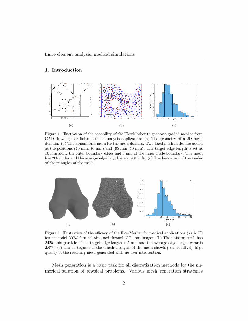
Figure 1: Illustration of the capability of the FlowMesher to generate graded meshes fromCAD drawings for finite element analysis applications (a) The geometry of a 2D meshdomain. (b) The nonuniform mesh for the mesh domain. Two fixed mesh nodes are addedat the positions (70 mm, 70 mm) and (95 mm, 70 mm). The target edge length is set as10 mm along the outer boundary edges and 5 mm at the inner circle boundary. The meshhas 206 nodes and the average edge length error is 0.55%. (c) The histogram of the anglesof the triangles of the mesh.
(a) (b) (c)
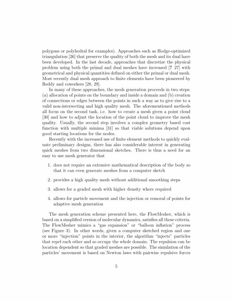
Figure 2: Illustration of the efficacy of the FlowMesher for medical applications (a) A 3Dfemur model (OBJ format) obtained through CT scan images. (b) The uniform mesh has2425 fluid particles. The target edge length is 5 mm and the average edge length error is2.0%. (c) The histogram of the dihedral angles of the mesh showing the relatively highquality of the resulting mesh generated with no user intervention.
Mesh generation is a basic task for all discretization methods for the nu-merical solution of physical problems. Various mesh generation strategies
2

have been deployed over the years [1, 2, 3] and have been successfully in-tegrated into commercial packages and are in widespread use in the finiteelement and finite volume community. The meshes applied in numericalsimulations are generally classified into two categories: structured and un-structured meshes. Since unstructured meshes provide better conformityto complex geometries than structured meshes [4], unstructured meshes aremore suitable to be used in medical simulations where the geometries of meshdomains are typically very complex.
Surgical simulation is a modern methodology for training students andprofessionals in surgical interventions. Real-time rendering technology andhaptic devices based on high-fidelity surgical simulators have been adopted bythe surgical community. Once surgical simulators are developed, the train-ing scenarios are rarely updated by healthcare educators due to a lack ofexpertise in numerical simulations. Allowing medical educators to set newsimulation scenarios is extremely valuable, because even for the same typeof surgery there can be many different training scenarios since human organsand tissues change with ages and patients can have many different symp-toms. For example, the procedures of surgeries to cure stomach cancers canbe different according to the geometries as well as the positions of tumors instomachs and patients’ age. However, it is not possible to develop surgicalsimulators by engineers that cover all the practical scenarios due to the limitof funding resources and an unlimited number of cases in reality.
A prospective technical plan is to develop a surgical simulator that an ed-ucator can adjust the existing training scenarios or even create new trainingscenarios without the need for expertise in numerical simulations. To developsuch a simulator, it is essential to integrate an automatic mesh generator togenerate meshes for objects on which learners practice. Unstructured meshesare widely adopted in medical simulation [5]. Furthermore, compared to theautomatically structured meshes generation algorithms, automatically un-structured meshes algorithms are generally simpler to be achieved [6]. Thiswork aims to develop an automatic unstructured mesh generator that caneasily be integrated into surgical simulators, which allows healthcare educa-tors to adjust and create training scenarios.
Automatically unstructured mesh generation methods is an active re-search subject in recent decades. Delaunay triangulation based methodsand its variations [7, 8, 9], advancing front methods [10, 11], Octree-basedmethods [12, 13], and their hybrid methods [14, 15] are the most popular au-tomatically mesh generation methods. However, these geometrically based
3

methods, particularly extending the methods from 2D domain to 3D domain,require extensive mathematical descriptions of the objects.
Besides the above geometrically based mesh generation methods, thereare some physically based mesh generators, such as the bubble mesh [16].Bubble mesh is an approach that is based on sphere packing, i.e. it consid-ers each node to be a solid sphere and packs them inside the mesh domain.However, it requires a good initial bubble configuration to reduce the con-vergence in the relaxation stage. Moreover, the adaptive population controlmechanism of the bubble mesh cannot be parallelized [17]. Therefore Bubblemesh cannot fully benefit from parallelization, which is a key approach toimprove the mesh generating efficiency in other methods.
Smoothed-particle hydrodynamics (SPH) [18] based mesh generation al-gorithms [19, 20] are recent methods to automatically generate unstructuredmeshes. They are based on a level set description of a surface and requirea background multi-resolution Cartesian mesh assigning boundary points,seeding it with interior points and then improving on their locations usingthe equations for fluid flow. In addition, assigning mesh nodes on bound-ary edges or surfaces of mesh domains and using temporal ghost particles atthe boundaries can complicate the implementation of the mesh generationmethods or even reduce the efficiency.
The above approaches require the use of the expertise of varying degrees todevelop meshes. Instead of developing mesh generators, it is possible to inte-grate open source mesh generation methods into medical simulators, such asDistMesh [21], PolyMesher [22], and Gmsh [23], which are very popular in thefinite element methods community. DistMesh is also a physically based meshgenerator and requires knowledge of distance functions for bounding surfaceswhich are very challenging for complex domains. Additionally, DistMesh andPolyMesher are written in MATLAB, which is not a popular programminglanguage for developing surgical simulators. Gmsh uses a local refinementstrategy starting from the Delaunay triangulation of the boundary pointsand then adding new points as required, and requires user interventions touse it.
There has also been a considerable effort focused on the fast triangulationof domains using techniques such as optimal Delaunay triangulation [24]or centroidal Voronoi tessellation [25]. These techniques have seen furtherimpetus due to applications of discrete differential geometry which requiresboth the original mesh (the triangles or tetrahedral obtained as a result ofa Delaunay triangulation for instance) as well as its dual (the Voronoi cell
4
polygons or polyhedral for examples). Approaches such as Hodge-optimizedtriangulation [26] that preserve the quality of both the mesh and its dual havebeen developed. In the last decade, approaches that discretize the physicalproblem using both the primal and dual meshes have increased [? 27] withgeometrical and physical quantities defined on either the primal or dual mesh.Most recently dual mesh approach to finite elements have been pioneered byReddy and coworkers [28, 29].
In many of these approaches, the mesh generation proceeds in two steps:(a) allocation of points on the boundary and inside a domain and (b) creationof connections or edges between the points in such a way as to give rise to avalid non-intersecting and high quality mesh. The aforementioned methodsall focus on the second task, i.e. how to create a mesh given a point cloud[30] and how to adjust the location of the point cloud to improve the meshquality. Usually, the second step involves a complex geometry based costfunction with multiple minima [31] so that viable solutions depend upongood starting locations for the nodes.
Recently with the increased use of finite element methods to quickly eval-uate preliminary designs, there has also considerable interest in generatingquick meshes from two dimensional sketches. There is thus a need for aneasy to use mesh generator that
1. does not require an extensive mathematical description of the body sothat it can even generate meshes from a computer sketch
2. provides a high quality mesh without additional smoothing steps
3. allows for a graded mesh with higher density where required
4. allows for particle movement and the injection or removal of points foradaptive mesh generation
The mesh generation scheme presented here, the FlowMesher, which isbased on a simplified version of molecular dynamics, satisfies all these criteria.The FlowMesher mimics a “gas expansion” or “balloon inflation” process(see Figure 3). In other words, given a computer sketched region and oneor more “injection” points in the interior, the algorithm “injects” particlesthat repel each other and so occupy the whole domain. The repulsion can belocation dependent so that graded meshes are possible. The simulation of theparticles’ movement is based on Newton laws with pairwise repulsive forces
5

and velocity based drag forces constraints that allows particles to dissipatetheir kinetic energy.
The fluid particles are prevented from crossing any boundary so thatthey eventually occupy the region assigned to them with maximally separatedistances. If new particles are injected, they will simply readjust based onthe repulsive forces. If the boundaries move they will exert “forces” on theparticles which will consequently readjust. With this approach, it is shownthat we obtain excellent mesh quality with minimal user intervention.
Figure 3: (a) The plot of a 2D object represents the mesh domain, which is assumed tobe a watertight container. (b) Mesh nodes are assumed to be fluid particles, which areinjected at multiple places and can flow inside the container. (c) The fluid particles aredistributed over the container until the flow is stopped (the speed of the fluid particlesis very small). (d) Generate a mesh based on the positions of the fluid particles usingDelaunay triangulation.
The major innovations of the FlowMesher are
1. the algorithm does not require initial mesh nodes configuration, whichis required in other physically based mesh generation methods, such asthe bubble mesh [16] and the DistMesh [21].
2. compared to SPH based mesh generators [19, 20], which also simulate
6

the flow of fluid particles, the FlowMesher is much easier to be imple-mented, because (1) the calculation of repelling and viscous forces inthis work is only based on kernel functions and fluid particles’ velocitieswithout the need for calculating the gradient of pressure and velocities;(2) the FlowMesher does not require the sampling of mesh nodes be-fore the flow simulation and assigning mesh nodes on boundary edges(for 2D mesh domain) and boundary surfaces (for 3D mesh domain),which are essentially tasks for generating meshes for 2D curves and 3Dsurfaces respectively, (3) the FlowMesher does not need to calculateghost boundary mesh nodes, which take extra memories.
3. the flow simulation always converges since considering mass and simu-lation time step size in the viscous forces guarantees that the viscousforces keep trying to dissipate the kinetic energy of fluid particles;
4. the algorithm can easily handle fixed mesh nodes constraints;
5. the mesh nodes number estimation algorithm automatically updatesthe number of fluid particles according to the error between the elementsize of a resulting mesh and its target size; therefore the FlowMesherdoes not require a predetermined number of mesh nodes.
In the following section, we first introduce the algorithm that can be usedto generate a uniform unstructured mesh.
2. Uniform simplex mesh
The mesh generation algorithm, the FlowMesher, includes two main steps:(1) obtain fluid particles’ distribution over a mesh domain; (2) generate amesh based on the fluid particles’ positions using Delaunay triangulation.While the second part is fairly routine, the first part is where the innovationsand simplicity of the algorithm lies. The overview of the algorithm to obtainthe fluid particles’ position is shown in Table 1. The details are discussed inthe following part.
2.1. Initialization
At the initial step, 2D and 3D mesh domains represented by triangularmeshes (see Figure 4 as an example of a 2D mesh domain) following the OBJfile format are prepared. Then the simulation parameters, such as the total
7

Table 1: The overview of the FlowMesher to obtain the positions of fluid particles.
1 Initialization1.1 Prepare a mesh domain composed of pure triangles in OBJ for-
mat.1.2 Set simulation parameters: the mesh size function h(x) = h,
total simulation time Ttotal, time step size ∆t, and Nstatus =False.
1.3 Add extra vertices on the mesh domain boundaries to ensurethat fluid particles flow inside the mesh domain.
1.4 Calculate the initial target number of fluid particles Ntotal.1.5 Set injection positions S where fluid particles will be injected.1.6 (Optional) Set fixed mesh nodes.
2 While t < Ttotal (run the flow simulation):2.1 If Np < Ntotal:
Generate new fluid particles at the injection positions S.Else if Np > Ntotal:
Remove extra fluid particles.2.3 If multiple fluid particles overlap at the same position, keep one
and remove extra fluid particles.2.4 Update the fluid particles’ positions according to equation (3).2.5 If a fluid particles’ flow outside of the mesh domain, project the
fluid particle on the boundary.2.6 Calculate the average distance ∆dti that the fluid particles travel
at the current time step ti.2.7 Find ∆dmax = max(∆d1,∆d2, · · · ,∆dti).2.8 If
∆dti∆dmax
< 5% & Np = Ntotal & Nstatus = False:
Update Ntotal and set Nstatus = True
2.9 If∆dti
∆dmax> 6%:
Set Nstatus = False
2.10 If∆dti
∆dmax< 0.5% & Np = Ntotal:
Terminate the flow simulation3 The positions of the fluid particles can be used to generate a mesh.
simulation time Ttotal, the time step size ∆t, and mesh size function over themesh domain h(x), are set. Since the mesh is uniform, the mesh size functionis set as h(x) = h (h is a constant).
8

Figure 4: The triangular mesh following the OBJ format represents a 2D mesh domain.The solid line segments are the boundary edges. Ai and Ci are the area and centroid ofthe ith triangle of the mesh domain respectively.
2.1.1. Estimate the target number of fluid particles
For a 2D mesh domain represented by a triangular mesh in OBJ fileformat, the initial target number of fluid particles that will be injected intothe mesh domain can be estimated as,
Ntotal =A2d
6A0
+L2d
h(1)
where A2d is the total area of the mesh domain; L2d is the total length ofthe boundary edges; A0 =
√3
4h2 is the area of an equilateral triangle with
edge length h. The estimated fluid particles are composed of two parts, thefluid particles inside the mesh domain and the ones on the boundary of themesh domain. As shown in Figure 5, each mesh node can be shared by sixtriangles at maximum for an ideal mesh; thus the estimated number of thefluid particles inside the mesh domain is set as A2d
6A0(see the first term of the
right hand side of equation (1)). Because there are approximately Lh
nodeson a boundary edge with the length L, the estimated number of the fluidparticles on the boundary of the mesh domain is set as L2d
hin the second
term of the right hand side of equation (1).For a 3D mesh domain represented by a triangular surface mesh in OBJ
9

Figure 5: The dots represent mesh nodes. The solid line segments draw an ideal meshcomposed of six equilateral triangles with edge length h and the area of each triangle is√
34 h
2. Each node can be shared by six triangles at maximum of the ideal mesh.
file format, the initial target number of fluid particles is estimated as,
Ntotal =V3d
18V0
+A3d
6A0
(2)
where A3d is the surface area of the 3D mesh domain; V3d is the volume ofthe 3D mesh domain; V0 = h3
6√
2is the volume of a regular tetrahedron with
edge length h, and A0 =√
34h2. Similar to the 2D case, the estimated fluid
particles are composed of two parts, the fluid particles inside the 3D meshdomain and the ones on the boundary surface of the 3D mesh domain. Weassume that a mesh node can be shared by 18 tetrahedrons at maximum formost meshes; therefore, the estimated number of fluid particles inside the 3Dmesh domain is set as V3d
18V0. The estimated number of fluid particles on the
boundary surface of the 3D mesh domain is set as A3d
6A0, which is the same as
the estimated number of fluid particles inside the 2D mesh domain.It is worth noting that the estimated number of fluid particles is under-
estimated for both 2D and 3D mesh domains at the initialization step, morefluid particles will be injected during the flow simulation.
2.1.2. Initialize the positions of fluid particle sources
The essential feature of the approach (and one that makes it differentthan other approaches in the literature), is the fact that rather than pre-distributing fluid particles (or mesh nodes) which is a complicated task, wejust select a few points (it could be as low as one) in the interior to injectfluid particles and let the repulsion between the fluid particles force them todistribute themselves throughout the domain.
10

The positions of fluid particle injection positions S, where the fluid par-ticles are injected, can either be manually set by users or be calculated auto-matically based on the geometry of the mesh domain and mesh size function.The algorithm to calculate fluid particle injection positions S for a 2D meshdomain is shown in Table 2. Ntri is the total number of triangles of the 2Dmesh domain. Ai and Ci are the area and centroid of the ith triangle of the2D mesh domain (see Figure 4). Using the algorithm shown in Table 2, wecan obtain the fluid particles’ injection positions, S = {S1,S2, · · · ,SNs} (Ns
is the number of the injection positions).
Table 2: The algorithm to calculate fluid particle injection positions for a 2D mesh domain.
1 Let Asum = 0, j = 1, A0 =√
34h2 .
2 For i = 1, 2, · · · , Ntri:2.1 Asum = Asum + Ai:2.2 If Asum ≥ 6.0A0:
Calculate the centroid of the ith triangle Ci.The centroid Ci is the jth fluid particle resource, Sj = Ci.Let Asum = 0, j = j + 1.
3 S = {S1,S2, · · · ,SNS} are the Ns = j − 1 fluid particle resources.
The algorithm to calculate the injection positions S for a 3D mesh domainis similar to the 2D case and is not discussed here (see Appendix A for thedetails).
2.1.3. Set fixed mesh nodes
The FlowMesher can easily handle fixed mesh nodes constraints by spec-ifying the positions of fixed fluid particles. If Nf fixed mesh nodes are set atthe positions F = {F1,F2, · · · ,FNf
}, fluid particles (speeds are set as zeros)are immediately injected at these positions before the simulation of the fluidparticles’ flow. The method to handle the fixed fluid particles is very simpleand straight forward, and is discussed in section 2.2.1.
Up to now, the initialization is completed and the simulation of the fluidparticles’ flow is introduced as follows.
2.2. Simulation of the fluid particles’ flow
At the beginning of the simulation of the fluid particles’ flow, we com-pare the current number of fluid particles Np and the target number of fluidparticles Ttotal.
11
• If Np < Ttotal: new fluid particles are injected at the injection positionsS. For each time step, only one fluid particle is allowed to be injectedat one fluid source position. Therefore, the maximum number of fluidparticles that can be injected at each time step is Ns.
• If Np > Ttotal: the recently injected Np − Ttotal fluid particles are re-moved at the current time step.
The direction of the initial velocity of a fluid particle is chosen at randomso that the particles are distributed throughout the domain with a verylow probability of collision. The overlap between the fluid particles is thenchecked. If multiple fluid particles are overlapped at one location, extra fluidparticles are removed and only one fluid particle is kept at this location.
2.2.1. Update the positions of the fluid particles
The positions of the fluid particles are updated based on the Euler methodthrough the following governing equation,
mxi(t+ ∆t) = Ffi(x(t)) + Fvi(x(t))
xi(t+ ∆t) = xi(t) + xi(t+ ∆t)∆t
xi(t+ ∆t) = xi(t) + xi(t+ ∆t)∆t
(3)
where xi is the position of the ith fluid particle pi; the mass m of a fluidparticle is a constant; Ffi is the fluid repelling force applied on pi,
Ffi = ks
Ni∑j=1
W
(||xi − xj||
h
)xi − xj
||xi − xj||(4)
xj are the positions of the pi’s neighbor fluid particles; Ni the total numberof the neighbor fluid particles; the kernel function W (q)
W (q) = α
(2− q)3 − 4(1− q)3 0 ≤ q < 1
(2− q)3 1 ≤ q < 2
0 q ≥ 2
(5)
is a modification of the kernel function in the work [32]. In this work, the
kernel width is set as the target mesh size h and therefore q =‖xi−xj‖
h; α is
set as α = 16
for 2D case and α = 118
for 3D case. Once the distance between
12

two fluid particles at xi and xj is smaller than 2h, a repelling force can begenerated between these two particles. The viscous force Fvi is set as
Fvi = −kvmxi
∆t(6)
to stabilize the flow, and kv is a constant (0 < kv < 1). It is worth notingthat if there is no repelling force applied on the ith particle (Ffi = 0), theviscous force (6) can reduce the velocity of the ith fluid particle from xi to(1− kv)xi, which indicates xi(t+ ∆t) = (1− kv)xi(t). Therefore, the viscousforces always try to dissipate the kinetic energy of the fluid particles. Thebigger kv is set, the faster the flow is stopped. In this work, kv is set in therange of 0.05 ≤ kv < 0.1 and it works very well in all the simulations.
To handle the fixed mesh nodes constraints, we simply set the repellingforces and viscous forces applied on the fluid particles at F = {F1,F2, · · · ,FNf
}as zeros in the governing equation (3). Then the accelerations of the fixedfluid particles are equal to zero and so the positions of the fixed fluid particlesare never changed.
2.2.2. Project fluid particles that are outside mesh domains
If a fluid particle pi flow outside the mesh domain, the fluid particle willbe projected onto the boundary of the mesh domain, and the velocity isupdated as if the fluid particle is bouncing off the boundary of the meshdomain. The updated velocity is
xnewpi
= xpi − 2(xpi · np′i)np′i
(7)
where xpi and xnewpi
is the velocity of the fluid particle pi before and after pro-jection respectively; np′i
is the normal vector of the mesh domain boundarywhere the projection point p′i locates.
2.2.3. Update the target number of the fluid particles
During the simulation of the flow, at the end of each simulation time step,the average distance that the fluid particles travel is calculated as,
∆dti =1
Np
Np∑j=0
||xj(t+ ∆t)− xj(t)|| (8)
where ti is the time step number. ∆dmax is the maximum average distanceduring the simulation time,
∆dmax = max {∆dt0,∆dt1, · · · ,∆dti} (9)
13
If three criteria (1) ∆dti∆dmax
< 5% (the flow is considered to be relatively slow),(2) Np = Ntotal (the current number of the fluid particles Np is equal tothe target number Ntotal), and (3) Nstatus = False (if ∆dti
∆dmax> 6%, we set
Nstatus = False) are satisfied, the flow of the fluid particles is assumed to besmall; then the target number of fluid particles Ntotal is updated and Nstatus
is set as Nstatus = True.To update Ntotal, a mesh is generated based on the current fluid particles’
positions. The average edge length error of the mesh is obtained as,
eavg =1
Nedges
Nedges∑i=1
Li − hh
(10)
where Nedges is the total number of mesh edges; Li is the length of the ithedge. If the error between the averaged edge length and the target edgelength is greater than 0.02 (|eavg| > 0.02), the target number of the fluidparticles is updated as
e = sgn (eavg) ·min (kp · |eavg|, 0.25)
Ntotal(t+ ∆t) =
⌈Ntotal(t) (1 + e)
⌉(11)
where the constant kp is set as kp = 0.5 in this work. The algorithm to updatethe total number of fluid particles is similar to a proportional controller,and kp is the proportional term. To avoid big overshoot in a proportionalcontroller which may increase the convergence time in this work, the changein the number of the fluid particles is limited to 0.25Ntotal(t). If Np(t) <Ntotal(t + ∆t), more fluid particles will be added; if Np(t) > Ntotal(t + ∆t),extra fluid particles will be removed.
2.2.4. Terminate the flow simulation
If ∆dti∆dmax
< 0.5% and Np = Ntotal, the distances that fluid particles travelare very small and the flow is assumed to be stopped. Therefore the sim-ulation of the flow is terminated. A mesh will then be generated based onthe positions of the fluid particles using Delaunay triangulation. As themesh generation (given node distributions) is a routine procedure, it is notdiscussed in this work.
14
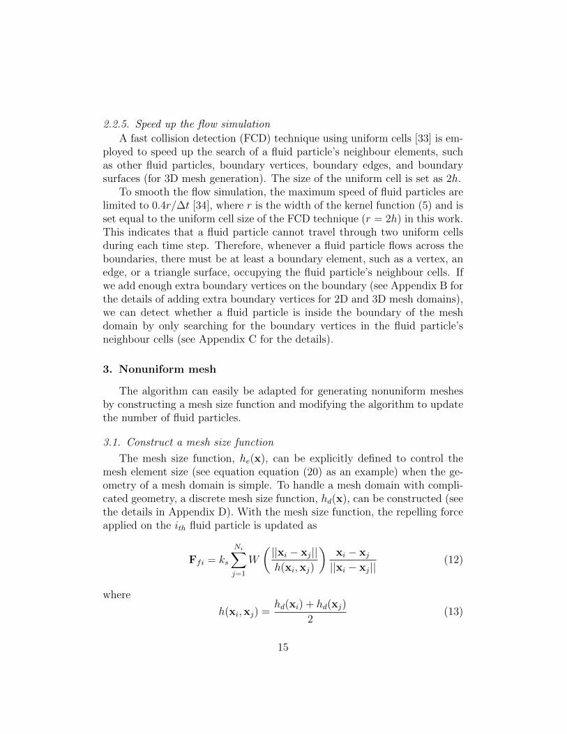
2.2.5. Speed up the flow simulation
A fast collision detection (FCD) technique using uniform cells [33] is em-ployed to speed up the search of a fluid particle’s neighbour elements, suchas other fluid particles, boundary vertices, boundary edges, and boundarysurfaces (for 3D mesh generation). The size of the uniform cell is set as 2h.
To smooth the flow simulation, the maximum speed of fluid particles arelimited to 0.4r/∆t [34], where r is the width of the kernel function (5) and isset equal to the uniform cell size of the FCD technique (r = 2h) in this work.This indicates that a fluid particle cannot travel through two uniform cellsduring each time step. Therefore, whenever a fluid particle flows across theboundaries, there must be at least a boundary element, such as a vertex, anedge, or a triangle surface, occupying the fluid particle’s neighbour cells. Ifwe add enough extra boundary vertices on the boundary (see Appendix B forthe details of adding extra boundary vertices for 2D and 3D mesh domains),we can detect whether a fluid particle is inside the boundary of the meshdomain by only searching for the boundary vertices in the fluid particle’sneighbour cells (see Appendix C for the details).
3. Nonuniform mesh
The algorithm can easily be adapted for generating nonuniform meshesby constructing a mesh size function and modifying the algorithm to updatethe number of fluid particles.
3.1. Construct a mesh size function
The mesh size function, he(x), can be explicitly defined to control themesh element size (see equation equation (20) as an example) when the ge-ometry of a mesh domain is simple. To handle a mesh domain with compli-cated geometry, a discrete mesh size function, hd(x), can be constructed (seethe details in Appendix D). With the mesh size function, the repelling forceapplied on the ith fluid particle is updated as
Ffi = ks
Ni∑j=1
W
(||xi − xj||h(xi,xj)
)xi − xj
||xi − xj||(12)
where
h(xi,xj) =hd(xi) + hd(xj)
2(13)
15

when a discrete mesh size function is constructed (or h(xi,xj) =he(xi)+he(xj)
2
for explicitly defined mesh size functions).
3.2. Update the number of the fluid particles
Similar to the uniform mesh algorithm, when the three criteria (1) ∆dtidmax
<5%, (2) Np = Ntotal, and (3) Nstatus = False are satisfied, a nonuniform meshis generated according to the positions of the fluid particles using Delaunaytriangulation. The average of edge length error of the mesh is then obtainedas,
eavg =1
Nedges
∑ ||xi − xj|| − h(xi,xj)
h(xi,xj)(14)
where Nedges is the total number of edges of the mesh; xi and xj are the twoends of a mesh edge; h(xi,xj) is target edge length (see equation (13)). Thenwe can insert eavg into equation (11) to obtain the updated target number offluid particles Ntotal(t+ ∆t).
4. Post-processing for 3D meshes
The FlowMesher algorithm distributes points throughout the domainmuch as gas will fill a region. Once the points are created a simple andfast Delaunay triangulation is employed to generate triangular meshes. TheFlowMesher coupled with Delaunay triangulation can generate high quality2D uniform and nonuniform meshes (see the details in the result section)without any further post-processing as can be seen in the results section.However, for 3-D meshes, the Delaunay triangulation has a tendency to cre-ate tetrahedrons that are of poor quality.
To determine whether a tetrahedron is of poor quality (or “unhealthy”),a quality index q defined by
q = 6√
6V
LmaxS(15)
is introduced to measure the quality of the tetrahedron [35]. V is the volumeof the tetrahedron; Lmax the length of the longest edge of the tetrahedron; Stotal area of the four faces of the tetrahedron. The value of q is in the range0 < q ≤ 1. For a regular tetrahedron, q = 1.0. For a flat unhealthy tetra-hedron, the quality value q is close to 0. Therefore, an easily implementedoptimization algorithm is developed to optimize the 3D meshes by movingpoints slightly and removing some other unhealthy tetrahedral is used.
16
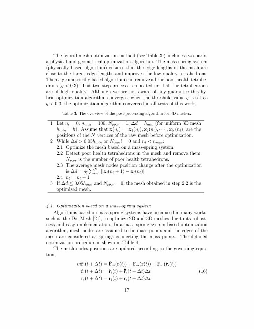
The hybrid mesh optimization method (see Table 3.) includes two parts,a physical and geometrical optimization algorithm. The mass-spring system(physically based algorithm) ensures that the edge lengths of the mesh areclose to the target edge lengths and improves the low quality tetrahedrons.Then a geometrically based algorithm can remove all the poor health tetrahe-drons (q < 0.3). This two-step process is repeated until all the tetrahedronsare of high quality. Although we are not aware of any guarantee this hy-brid optimization algorithm converges, when the threshold value q is set asq < 0.3, the optimization algorithm converged in all tests of this work.
Table 3: The overview of the post-processing algorithm for 3D meshes.
1 Let nt = 0, nmax = 100, Npoor = 1, ∆d = hmin (for uniform 3D meshhmin = h). Assume that x(nt) = [x1(nt),x2(nt), · · · ,xN(nt)] are thepositions of the N vertices of the raw mesh before optimization.
2 While ∆d > 0.05hmin or Npoor! = 0 and nt < nmax:2.1 Optimize the mesh based on a mass-spring system.2.2 Detect poor health tetrahedrons in the mesh and remove them.
Npoor is the number of poor health tetrahedrons.2.3 The average mesh nodes position change after the optimization
is ∆d = 1N
∑Ni=1 ||xi(nt + 1)− xi(nt)||
2.4 nt = nt + 13 If ∆d ≤ 0.05hmin and Npoor = 0, the mesh obtained in step 2.2 is the
optimized mesh.
4.1. Optimization based on a mass-spring system
Algorithms based on mass-spring systems have been used in many works,such as the DistMesh [21], to optimize 2D and 3D meshes due to its robust-ness and easy implementation. In a mass-spring system based optimizationalgorithm, mesh nodes are assumed to be mass points and the edges of themesh are considered as springs connecting the mass points. The detailedoptimization procedure is shown in Table 4.
The mesh nodes positions are updated according to the governing equa-tion,
mri(t+ ∆t) = Fsi(r(t)) + Foi(r(t)) + Fdi(ri(t))
ri(t+ ∆t) = ri(t) + ri(t+ ∆t)∆t
ri(t+ ∆t) = ri(t) + ri(t+ ∆t)∆t
(16)
17

Table 4: The overview of the optimization algorithm based on a mass-spring system.
1 Generate a new mesh according to the position of the current meshnodes positions. Let t = 0, ∆d1 = hmin, r(0) the positions of themesh nodes, Ttotal = 100.0 the total optimization time, ∆t = 0.5 thetime step size.
2 while ∆d1 > 0.05hmin and t ≤ Ttotal:2.1 Update the position according to the governing equation (16)
2.2 The average distance change is ∆d1 = 1N
∑Ni=1 ||ri(t+∆t)−ri(t)||.
2.3 t = t+ ∆t3 The mesh is optimized and r(t) is the updated positions of the mesh
nodes.
in equation (17) above, Fsi is the spring force term
Fsi =
Nsi∑j=1
ks[lij − h(ri, rj)]eij (17)
where h(ri, rj) is the target edge length given in equation (13); lij = ||ri−rj||;eij = (rj − ri)/lij; ks a spring constant. ri and rj are the two ends of a meshedge. Fsi is the force that repels two nodes away if the edge length connectingthe two nodes smaller than the target edge length, and attracts two nodescloser if the edge length is greater than the target edge length.
Foi(r(t)) is a force applied on a node of an unhealthy tetrahedron withthe q value in the range of 0.3 ≤ q ≤ 0.5. Foi(r(t)) is discussed through an
Figure 6: The tetrahedron is a poor health tetrahedron. θbd is the dihedral angle betweentriangles Tabd and Tbcd, and θac is the dihedral angle between Tabc and Tacd. Assume thatθbd and θac are the largest two angles among the six dihedral angles of the tetrahedron.lpq is the shortest distance between edge Eac and Ebd.
example shown in Figure 6. θbd is the dihedral angle between triangles Tabdand Tbcd, and θac is the dihedral angle between Tabc and Tacd. Assume thatθbd and θac are the largest two angles among the six dihedral angles of the
18

tetrahedron. The force applied on node a is
Foa(r(t)) = ks(haim − lpq)epq +∑j
ks[laj − h(ra, rj)]eaj (18)
where haim =√
23[h(ra, rb)+h(rc, rd)], lpq = ||rp−rq||, epq = rq−rp
lpq, j = b, c, d,
laj = ||ra − rj||, eaj =rj−ralaj
. It is worth noting that the first term on the
right hand side of equation (18) is set to increase the distance between edgeEac and Ebd, and the second term is a force that try to make the length of theedge Eab, Eac, and Ead equal to their target edge lengths. The force appliedon the other three nodes can be obtained in a similar way. Therefore, Foi isa force applied on the ith mesh node of a poor health tetrahedron to improvethe tetrahedron quality.
4.2. Remove poor health tetrahedrons
The mass-spring system based optimization algorithm is only used toimprove the quality of tetrahedrons with the quality value q in the range of[0.3, 0.5]. In this part, we will remove tetrahedrons with the quality value ofq in the range of (0.0, 0.3) by projecting the four nodes of the tetrahedronsonto a plane. The algorithm is shown in Table 5.
Table 5: The optimization algorithm to remove poor health tetrahedrons.
1 Let N1i = 0, ∆d2(0) = hmin, r(0) = r(t).2 while ∆d2! = 0 and N1i < 10:
2.1 Update the 3D mesh based on the current particles’ positionsr(N1i).
2.2 For each tetrahedron of the mesh, if a tetrahedron quality valueis smaller than 0.3 (q < 0.3), project four vertices of the tetra-hedron onto a plane (see section 4.2 for the details). r(N1i + 1)is the updated position.
2.3 ∆d2 = 1N
∑Ni=1 ||ri(N1i + 1)− ri(N1i)||
2.4 N1i = N1i + 13 If ∆d2 = 0, the mesh is optimized and all the tetrahedrons with q in
the range of (0.0, 0.3) are removed.
In the post optimization process, the boundary mesh nodes and the nodesat predefined positions are considered to be fixed, and all the other nodes
19
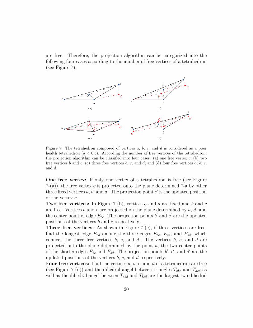
are free. Therefore, the projection algorithm can be categorized into thefollowing four cases according to the number of free vertices of a tetrahedron(see Figure 7).
Figure 7: The tetrahedron composed of vertices a, b, c, and d is considered as a poorhealth tetrahedron (q < 0.3). According the number of free vertices of the tetrahedron,the projection algorithm can be classified into four cases: (a) one free vertex c, (b) twofree vertices b and c, (c) three free vertices b, c, and d, and (d) four free vertices a, b, c,and d.
One free vertex: If only one vertex of a tetrahedron is free (see Figure7-(a)), the free vertex c is projected onto the plane determined 7-a by otherthree fixed vertices a, b, and d. The projection point c′ is the updated positionof the vertex c.Two free vertices: In Figure 7-(b), vertices a and d are fixed and b and care free. Vertices b and c are projected on the plane determined by a, d, andthe center point of edge Ebc. The projection points b′ and c′ are the updatedpositions of the vertices b and c respectively.Three free vertices: As shown in Figure 7-(c), if three vertices are free,find the longest edge Ecd among the three edges Ebc, Ecd, and Ebd, whichconnect the three free vertices b, c, and d. The vertices b, c, and d areprojected onto the plane determined by the point a, the two center pointsof the shorter edges Ebc and Ebd. The projection points b′, c′, and d′ are theupdated positions of the vertices b, c, and d respectively.Four free vertices: If all the vertices a, b, c, and d of a tetrahedron are free(see Figure 7-(d)) and the dihedral angel between triangles Tabc and Tacd aswell as the dihedral angel between Tabd and Tbcd are the largest two dihedral
20

angels among the six dihedral angels of the tetrahedron, the vertices a, b,c, and d are projected onto the plane which is determined by the centroidof the tetrahedron and a normal vector perpendicular to edges Eac and Ebd.The projection points are the updated positions of the vertices.
5. Results
5.1. 2D meshes
(a) (b)
(c) (d)
Figure 8: (a) Uniform mesh for a rectangular mesh domain. The mesh has 74 nodesand the average edge length is 10.07 mm and the target edge length is 10 mm. (b) Thenonuniform mesh for the rectangular mesh domain. The mesh has 64 nodes. The targetedge length is set as 10 mm at the boundary edge, and 20 mm at the centroid. The averageerror is 0.54%. (c) and (d) The histograms of the angles of the triangles in mesh (a) and(b) respectively.
Figure 8 shows two meshes for a rectangular mesh domain with a dimen-sion of 100 mm× 50 mm. In Figure 8-(a), the target length is set as 10 mm.The resulting uniform mesh has 74 nodes and the average edge length is 10.07mm (the average edge length error is 0.7%). In Figure 8-(b), the target edge
21

length of the mesh is set as 10 mm at the boundary edges of the rectangularshape and 20 mm at the centroid of the rectangular. The resulting mesh has64 nodes and the average edge length error is eavg = 0.54%. Figure 8-(c) and(d) shows the histograms of the angles of the triangles in mesh (a) and (b)respectively.
Figure 9 shows three meshes for an L-shape mesh domain. In Figure 9-a,the target edge length is set as 10 mm. The resulting mesh has 35 nodesand the average edge length is 10.42 mm. At the position of (10 mm, -10mm), the mesh does not match the geometry of the L-shape mesh domain.To solve this issue, fixed points can be defined before generating a mesh. For
(a) (b) (c)
(d) (e) (f)
Figure 9: (a) Uniform mesh for an L-shape mesh domain. The mesh has 35 nodes. Thetarget edge length is 10.00 mm and the average edge length is 10.42 mm. (b) Uniformmesh for the L-shape mesh domain. The mesh has 36 nodes. The target edge length is10.00 mm and the average edge length is 10.23 mm. A fixed mesh node is added at theposition of (10 mm, -10 mm). (c) The nonuniform mesh for the L-shape mesh domain.The mesh has 67 nodes. The target edge length is set as 10 mm at the boundary edgesEab, Ebc, Ecd, and Ede, and 2 mm at the position of (10 mm, -10 mm), where a fixed meshnode is added. The average edge length error is 1.99%. (d), (e) and (f) are the histogramsof the angles of the triangles in mesh (a), (b), and (c) respectively.
example, in Figure 9-b, a fixed mesh node is set at the position of (10 mm,
22

-10 mm). The resulting mesh has 36 nodes and the average edge length isequal to 10.23 mm. Figure 9-c shows the nonuniform mesh, which has 67nodes. The target edge length is set as 10 mm at the boundary edges Eab,Ebc, Ecd, and Ede, and 2 mm at the fixed mesh node locating at (10 mm, -10mm). The average edge length error is 1.99%.
To further demonstrate that the FlowMesher can handle complex meshdomains, a 2D nonuniform mesh is generated for a mesh domain shown inFigure 1-a. The target edge length is set as 10 mm along the outer boundaryedges and 5 mm at the inner boundary circle. Two fixed nodes are added atthe positions of (70 mm, 70 mm) and (95 mm, 70 mm). As shown in Figure1-b, the resulting mesh has 206 nodes and the average edge length error is0.55%. The histogram of the angles of the mesh triangles is shown in Figure1-c.
In the above 2D uniform and nonuniform triangular meshes, all the anglesof the meshes are fall in the range of [30, 100] degrees. Therefore, there areno bad triangles in the meshes. Even without post-processing algorithms,the 2D triangular meshes are of high quality.
5.2. 3D objects
In this work, truss structure objects are used to demonstrate 3D meshes.Each cylinder object of a truss structure represents an edge of a 3D mesh. Asshown in Figure 10, an uniform mesh is generated for a cuboid mesh domainwith the dimension 100 mm × 100 mm × 80 mm. The mesh has 258 nodesand the average edge length error is -0.02%. Figure 10-b shows the dihedralangles of the mesh.
The truss structure in Figure 11-a represents a nonuniform mesh for acylinder mesh domain with the dimension 50 mm (radius) × 40 mm (height).To control edge lengths functions, we define the target edge length as,
h(xi,xj) =he(xi) + he(xj)
2(19)
where he(x) is a explicitly defined mesh size function
he(x) = he([x, y, z]) =
(
1− 0.4
√x2 + y2
35.0
)r if
√x2 + y2 < 35.0
0.6r if√x2 + y2 ≥ 35.0
(20)
where r = 25 mm. Three fixed nodes are added along the axis of the cylinder(two nodes on the circular bases and one node is at the centroid of the
23

(a) (b)
Figure 10: (a) Uniform mesh for a cuboid with the dimension 100 × 100 × 80 mm. Themesh has 258 fluid particles. The target edge length is 20 mm. The average edge lengtherror is -0.02%. (b) The histogram of the dihedral angles of the mesh.
cylinder). The resulting mesh has 545 fluid particles and the average edgelength error is 1.54 %. Figure 11-b shows the histogram of the dihedral anglesof the mesh.
A uniform mesh shown in Figure 12 for a shoe sole mesh domain witha thickness of 14 mm has 1117 nodes. The mesh domain is developed byscanning a shoe using a 3D scanner. The target edge length is set as 9 mmand the average edge length of error of the mesh is 0.75%. The mesh nodesare clear distributed in three layers (see Figure 12-b). Figure 12-c shows thehistogram of the dihedral angles of the mesh.
Figure 2-a shows a piece of a 3D femur model in OBJ format, and the 3Dmodel is obtained through CT scan images. Figure 2-b shows the uniformtetrahedron mesh generated for the 3D mesh domain represented by the3D femur model. The uniform mesh has 2425 fluid particles. The targetedge length is 5 mm and the average edge length error is 2.0%. Figure 2-c is the histogram of the dihedral angles θDihedral of the tetrahedron mesh.This example shows the potential that the FlowMesher algorithm can beintegrated into a medical simulator to automatically generate meshes formedical simulations.
For all the 3D meshes generated in the above, the average edge lengtherrors are all smaller than 2%. Meanwhile, more than 97% dihedral anglesare in the range of [30, 150] degrees. There are only a few dihedral anglessmaller than 30◦ but greater than 12◦, and less than 0.5% dihedral angles
24

(a)
(b)
Figure 11: (a) Nonuniform mesh for a cylinder mesh domain with the dimension 50 mm(radius) × 40 mm (height). The mesh has 545 nodes and the average edge length error is1.54%. The middle and right figures are the views of the cross sections of the mesh. (b)The histogram of the dihedral angles of the mesh.
that are in the range of [150, 165] degrees. Therefore, the average edge lengthis accurately controlled and there are no flatten tetrahedrons in the meshesgenerated in this work.
6. Conclusion
The FlowMesher proposed in this work should be one of the simplest au-tomatic mesh generation algorithms that can be used to generate isotropicunstructured mesh for an object in any shape in an automatic way with min-imum (or even no) user intervention. The performance of the FlowMesheris demonstrated by generating meshes for several 2D and 3D mesh domains.The results show that the qualities of the meshes are good and the accuracyof edge length can be guaranteed. Particularly, no post-processing procedureis required for generating high quality 2D triangular meshes. The fluid par-
25

(a)
(b) (c)
Figure 12: (a) Uniform mesh for an insole shape. The mesh has 1117 fluid particles andthe average edge length error is 0.75%. (b) The distribution of the fluid particles. (c) Thehistogram of the dihedral angles of the mesh.
ticles’ flow simulation is guaranteed to converge to obtain the mesh nodesdistributions.
Creating 3D models using CT scan images and 3D scanned images iscommon in the medical healthcare community nowadays. Therefore, it iscompletely possible that a healthcare educator can provide 3D models re-quired in surgical training scenarios. In the future, we will develop a surgicalsimulator integrating the FlowMesher which is used to automatically gener-ate meshes for the 3D models to run the surgical simulation. Besides, wewill employ parallel computing techniques to improve the efficiency of theFlowMesher. The flow simulation of the FlowMesher and SPH share a lot ofsimilarities in technical details, such as searching for neighbour fluid particlesand the use of kernel functions, etc. Therefore, we will explore the parallelcomputing techniques for SPH based flow simulations to boost up the per-formance of the FlowMesher. Furthermore, other triangulation algorithmsand post-optimization algorithms will be investigated to link and move fluidparticles to generate tetrahedron meshes with better qualities. The ultimategoal is to publish the FlowMesher as an alternative open source mesh gener-ator.
26

Acknowledgments
The first and last authors gratefully acknowledge the support1 of the pro-gram of Canada Research Chair in Health Care Simulation. The second andthird authors acknowledge the support of their respective endowed profes-sorships.
References
[1] Steven J Owen. A survey of unstructured mesh generation technology.In Proceedings of 7th International Meshing Roundtable, pages 239–267.Sandia National Lab, October 1998.
[2] David Bommes, Bruno Levy, Nico Pietroni, Enrico Puppo, ClaudioSilva, Marco Tarini, and Denis Zorin. Quad-mesh generation and pro-cessing: A survey. In Computer Graphics Forum, volume 32, pages51–76. Wiley Online Library, 2013.
[3] Daniel S.H. Lo. Finite element mesh generation. CRC Press, 2014.
[4] Jonathan R. Shewchuk. Delaunay refinement mesh generation. PhDthesis, Carnegie-Mellon Univ Pittsburgh Pa School of Computer Science,1997.
[5] Michel A. Audette, Andrey N. Chernikov, and Nikos P. Chrisochoides.A review of mesh generation for medical simulators. In Handbook ofReal-World Applications in Modeling and Simulation, pages 261–297.Wiley Online Library, 2012.
[6] Valerie Mounoury and Olivier Stab. Automatic quadrilateral and hexa-hedral finite element mesh generation: review of existing methods. RevueEuropeenne des Elements Finis, 4(1):75–102, 1995.
[7] Jim Ruppert. A Delaunay refinement algorithm for quality 2-dimensional mesh generation. J. Algorithms, 18(3):548–585, 1995.
[8] Jonathan Richard Shewchuk. Delaunay refinement algorithms for trian-gular mesh generation. Computational geometry, 22(1-3):21–74, 2002.
1This project was led by Zhujiang Wang as a part of post-doctoral studies supportedby Canada Research Chair in Health Care Simulation awarded to Adam Dubrowski.
27
[9] Panagiotis Foteinos and Nikos Chrisochoides. Dynamic parallel 3D De-launay triangulation. In Proceedings of the 20th International MeshingRoundtable, pages 3–20. Springer, 2011.
[10] Joachim Schoberl. NETGEN An advancing front 2D/3D-mesh gener-ator based on abstract rules. Computing and Visualization in Science,1(1):41–52, 1997.
[11] Fariba Mohammadi, Shusil Dangi, Suzanne M. Shontz, and Cristian A.Linte. A direct high-order curvilinear triangular mesh generationmethod using an advancing front technique. In International Conferenceon Computational Science, pages 72–85. Springer, 2020.
[12] Mark S. Shephard and Marcel K. Georges. Automatic three-dimensionalmesh generation by the finite octree technique. International Journalfor Numerical Methods in Engineering, 32(4):709–749, 1991.
[13] Mark A. Yerry and Mark S. Shephard. Automatic three-dimensionalmesh generation by the modified-octree technique. International Journalfor Numerical Methods in Engineering, 20(11):1965–1990, 1984.
[14] Dimitri J. Mavriplis. An advancing front delaunay triangulation al-gorithm designed for robustness. Journal of Computational Physics,117(1):90–101, 1995.
[15] Houman Borouchaki, Patrick Laug, and Paul-Louis George. Parametricsurface meshing using a combined advancing-front generalized Delaunayapproach. International Journal for Numerical Methods in Engineering,49(1-2):233–259, 2000.
[16] Kenji Shimada and David C. Gossard. Bubble mesh: automated triangu-lar meshing of non-manifold geometry by sphere packing. In Proceedingsof the third ACM symposium on Solid modeling and applications, pages409–419, 1995.
[17] Yves Marechal et al. GPU-based parallelization for bubble mesh gener-ation. COMPEL-The international journal for computation and math-ematics in electrical and electronic engineering, 36(4):1184–1197, 2017.
[18] Joe J. Monaghan. Smoothed particle hydrodynamics. Reports onProgress in Physics, 68(8):1703–1759, 2005.
28

[19] Lin Fu, Luhui Han, Xiangyu Y. Hu, and Nikolaus A. Adams. Anisotropic unstructured mesh generation method based on a fluid relax-ation analogy. Computer Methods in Applied Mechanics and Engineer-ing, 350:396–431, 2019.
[20] Zhe Ji, Lin Fu, Xiangyu Hu, and Nikolaus Adams. A feature-aware SPH for isotropic unstructured mesh generation. arXiv preprintarXiv:2003.01061, 2020.
[21] Per-Olof Persson and Gilbert Strang. A simple mesh generator in MAT-LAB. SIAM Review, 46(2):329–345, 2004.
[22] Cameron Talischi, Glaucio H. Paulino, Anderson Pereira, and Ivan F.M.Menezes. PolyMesher: a general-purpose mesh generator for polygonalelements written in Matlab. Structural and Multidisciplinary Optimiza-tion, 45(3):309–328, 2012.
[23] Christophe Geuzaine and Jean-Francois Remacle. Gmsh: A 3-D fi-nite element mesh generator with built-in pre-and post-processing fa-cilities. International Journal for Numerical Methods in Engineering,79(11):1309–1331, 2009.
[24] Long Chen and Jin-chao Xu. Optimal Delaunay triangulations. Journalof Computational Mathematics, 22(2):299–308, 2004.
[25] Qiang Du, Vance Faber, and Max Gunzburger. Centroidal Voronoitessellations: Applications and algorithms. SIAM Review, 41(4):637–676, 1999.
[26] Patrick Mullen, Pooran Memari, Fernando de Goes, and Mathieu Des-brun. HOT: Hodge-optimized triangulations. In ACM SIGGRAPH 2011Papers, SIGGRAPH ’11, New York, NY, USA, 2011. Association forComputing Machinery.
[27] Mathieu Desbrun, Eva Kanso, and Yiying Tong. Discrete differentialforms for computational modeling. In Discrete Differential Geometry,volume 38, pages 287–324. Springer, 2008.
[28] J.N. Reddy. A dual mesh finite domain method for the numerical solu-tion of differential equations. International Journal for ComputationalMethods in Engineering Science and Mechanics, 20(3):212–228, 2019.
29

[29] J.N. Reddy, Praneeth Nampally, and Arun R. Srinivasa. Nonlinear anal-ysis of functionally graded beams using the dual mesh finite domainmethod and the finite element method. International Journal of Non-Linear Mechanics, 127:103575, 2020.
[30] Leif P. Kobbelt and Mario Botsch. An interactive approach to pointcloud triangulation. In Computer Graphics Forum, volume 19, pages479–487. Wiley Online Library, 2000.
[31] Marshall Bern and David Eppstein. Mesh generation and optimal tri-angulation. Computing in Euclidean geometry, 1:23–90, 1992.
[32] Joseph J. Monaghan and John C. Lattanzio. A refined particle methodfor astrophysical problems. Astronomy and astrophysics, 149(1):135–143, 1985.
[33] Christer Ericson. Real-time collision detection. CRC Press, 2004.
[34] Damien Violeau and Agnes Leroy. On the maximum time step in weaklycompressible SPH. Journal of Computational Physics, 256:388–415,2014.
[35] Rocscience - mesh quality. https://www.rocscience.com/help/rs3/
Mesh/Mesh_Tools/Mesh_Quality.htm. Accessed: 2020-10-31.
Appendix A. Calculate the fluid particle injection positions for3D mesh domains
The algorithm to calculate fluid particle injection positions S for a 3Dmesh domain is shown in Figure A.13. A tetrahedron mesh M3d can begenerated based on the vertices of the triangular surface mesh representingthe 3D mesh domain using 3D Delaunay triangulation. Ntet is the totalnumber of tetrahedrons of the tetrahedron mesh M3d. V tet
i is the volumeof the ith tetrahedron. The volume summary of the tetrahedrons of M3d iscalculated iteratively. When the summation Vs is greater equal than 18Vt0after adding the volume of the ith tetrahedron V tet
i , the centroid Ci of thetetrahedron is added to the injection positions S and Vs is then set zero(Vs = 0). Repeat this process for all the tetrahedrons, the injection positionsS = {S1,S2, · · · ,SNs} is obtained and Ns is the total number of the injectionpositions of the fluid particles.
30

Figure A.13: The algorithm to calculate fluid particle injection positions. V teti is the
volume of the ith tetrahedron. Vt0 is set to equal Vt0 = h3
6√2. S are the injection positions
and Ns is the total number of S.
Appendix B. Adding extra boundary vertices for 2D and 3D meshdomains
Appendix B.1. Adding boundary vertices for 2D mesh domains
The method to add boundary vertices for a 2D mesh domain is demon-strated through an example shown in Figure B.14. The background uniformgrid drawn in dotted line segments is the uniform cells for the FCD tech-nique. A fluid particle p is flowing across the boundary edge Eab of the 2Dmesh domain. To detect whether the fluid particle p is near the boundaryof the 2D mesh domain, we search for the boundary vertices of the 2D meshdomain in the fluid particle p’s neighbour cells. However, since there is no
31

boundary vertex in the neighbour cells, we cannot detect that the fluid par-ticle p is near the boundary of the mesh domain. Therefore, the fluid particlep can flow outside the mesh domain without detection. To solve this kind of
Figure B.14: The background uniform grid drawn in dotted line segments is the uniformcells for the FCD technique. Extra vertices ab(1), ab(2), bc(1), cd(1), cd(2), and da(1)are added on the boundary edge. Since the boundary vertices ab(1) and ab(2) are in theneighbour cells of the fluid particle p, we can detect that the fluid particle p is near theboundary edge Eab of the 2D mesh domain.
problem, extra boundary vertices are added at
vab(i) = va +vb − va
Ne + 1· i, Nab =
⌈||vb − va||
4h− 1
⌉(B.1)
along the edge Eab, where i = 1, 2, ..., Nab, Nab the total number of extravertices added along the edge Eab. As a result, two extra vertices (Nab =2) ab(1) and ab(2) are added on the boundary edge Eab. When the fluidparticle p is crossing the edge Eab, the vertices ab(1) and ab(2) are in the fluidparticle’s neighbour cells and therefore we can use the two extra boundaryvertices ab(1) and ab(2) to detect that the fluid particle p is near the boundaryof the mesh domain.
Repeating this process for all the boundary edges of which the lengthis greater than 4h, extra boundary vertices bc(1), cd(1), cd(2), and da(1)are added onto the boundary edges Ebc, Ecd, and Eda. After adding theextra boundary vertices, since the maximum distance between two boundary
32
vertices on an edge is less equal than 4h and the uniform cell size for FCDis equal to 2h, whenever a fluid particle is near the boundary of the meshdomain, there must be at least one boundary vertices in the fluid particle’sneighbour cell. Thus, it is guaranteed that a fluid particle can be detectedwhen crossing a boundary edge.
Appendix B.2. Adding boundary vertices for 3D mesh domains
Similar to the 2D case, a fluid particle can flow across the boundary ofa 3D mesh domain through a boundary edge or triangle without detection.For example, a fluid particle p can crossing Tabc without detection (see FigureB.15-a). Therefore, extra boundary vertices are added on the boundary edgesand boundary triangles.
The method to add extra boundary vertices on the boundary of a 3Dmesh domain is discussed through the example shown in Figure B.15. Eab
is the longest edge and Ebc is the shortest. First, extra boundary vertices,such as vab(1), vab(2) on edge Eab, and vbc(1) on edge Ebc, are added on theboundary edges of the 3D domain using the same method for the 2D case(see Figure B.15-b). Extra vertices
vbc(i),ab(j) = vbc(i) +va − vb
Nab + 1j (B.2)
are then added on the plane of the triangle Tabc, where i = 1, 2, · · · , Nbc andj = 1, 2, · · · , Nab + 1; Nab = 2 and Nbc = 1 are the number of extra bound-ary vertices added on edges Eab and Ebc respectively. Therefore, vbc(1),ab(1),vbc(1),ab(2), and vbc(1),ab(3) are added (see Figure B.15-c). Additionally, theintersection points on edge Eca,
vbc(i),ca = xc +va − vc
Nbc + 1i (B.3)
where i = 1, 2, · · · , Nbc (in the case of Figure B.15-c, there is only one inter-section point vbc(1),ca). Removing the vertices outside the triangle Tabc (suchas the vbc(1),ab(1) and vbc(1),ab(2)) and the repeated vertices, the remaining ver-tices include three types: (1) vertices on edges such as vab(1), vab(2), vbc(1),vca(1), and vca(2); (2) vertices inside the triangle, such as vbc(1),ab(1); (3) inter-section points on edge Eca, such as vbc(1),ca (see Figure B.15-d). Repeatingthis process for all the boundary triangles, we can obtain all the extra bound-ary vertices on the boundary edges and surfaces of the 3D mesh domain. In
33
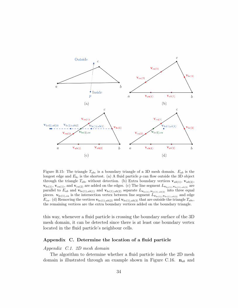
Figure B.15: The triangle Tabc is a boundary triangle of a 3D mesh domain. Eab is thelongest edge and Ebc is the shortest. (a) A fluid particle p can flow outside the 3D objectthrough the triangle Tabc without detection. (b) Extra boundary vertices vab(1), vab(2),vbc(1), vca(1), and vca(2) are added on the edges. (c) The line segment Lvbc(1),vbc(1),ab(3)
areparallel to Eab and vbc(1),ab(1) and vbc(1),ab(2) separate Lvbc(1),vbc(1),ab(2)
into three equalpieces. vbc(1),ca is the intersection vertex between line segment Lvbc(1),vbc(1),ab(3)
and edgeEca. (d) Removing the vertices vbc(1),ab(2) and vbc(1),ab(3) that are outside the triangle Tabc,the remaining vertices are the extra boundary vertices added on the boundary triangle.
this way, whenever a fluid particle is crossing the boundary surface of the 3Dmesh domain, it can be detected since there is at least one boundary vertexlocated in the fluid particle’s neighbour cells.
Appendix C. Determine the location of a fluid particle
Appendix C.1. 2D mesh domain
The algorithm to determine whether a fluid particle inside the 2D meshdomain is illustrated through an example shown in Figure C.16. nab and
34
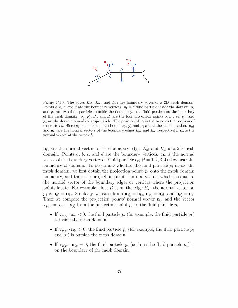
Figure C.16: The edges Eab, Ebc, and Ecd are boundary edges of a 2D mesh domain.Points a, b, c, and d are the boundary vertices. p1 is a fluid particle inside the domain; p2and p3 are two fluid particles outside the domain; p4 is a fluid particle on the boundaryof the mesh domain. p′1, p′2, p′3, and p′4 are the four projection points of p1, p2, p3, andp4 on the domain boundary respectively. The position of p′2 is the same as the position ofthe vertex b. Since p4 is on the domain boundary, p′4 and p4 are at the same location. nab
and nbc are the normal vectors of the boundary edges Eab and Ebc respectively. nb is thenormal vector of the vertex b.
nbc are the normal vectors of the boundary edges Eab and Ebc of a 2D meshdomain. Points a, b, c, and d are the boundary vertices. nb is the normalvector of the boundary vertex b. Fluid particles pi (i = 1, 2, 3, 4) flow near theboundary of domain. To determine whether the fluid particle pi inside themesh domain, we first obtain the projection points p′i onto the mesh domainboundary, and then the projection points’ normal vector, which is equal tothe normal vector of the boundary edges or vertices where the projectionpoints locate. For example, since p′1 is on the edge Ebc, the normal vector onp1 is np′1
= nbc. Similarly, we can obtain np′3= nbc, np′4
= nab, and np′2= nb.
Then we compare the projection points’ normal vector np′iand the vector
vp′ipi= xpi − xp′i
from the projection point p′i to the fluid particle pi.
• If vp′ipi·nbc < 0, the fluid particle pi (for example, the fluid particle p1)
is inside the mesh domain.
• If vp′ipi· nbc > 0, the fluid particle pi (for example, the fluid particle p2
and p3) is outside the mesh domain.
• If vp′ipi· nbc = 0, the fluid particle pi (such as the fluid particle p4) is
on the boundary of the mesh domain.
35

Figure C.17: The triangles are parts of a 3D object boundary. p1, p2, and p3 are threefluid particles outside the object. p′1, p′2, and p′3 are the three projection points of p1, p2,and p3 on the object respectively (the position of p′3 is the same as the position of thevertex c). vp′
ipi= xpi
−xp′i
(i = 1, 2, 3) are three vectors from the projection points to thefluid particles. nabc and nacd are the normal vector of triangles Tabc and Tacd respectively.nc is the normal vector of the vertex c on the object.
Appendix C.2. 3D mesh domain
The method to project fluid particles outside the 3D mesh domain ontoits boundary is similar to the method for the 2D mesh domain in the previouspart. When a fluid particle pi is near the boundary, we should obtain theprojection point p′i on the 3D mesh domain and the projection points’ normalvector. As shown in Figure C.17, a fluid particle’s projection point can beon a triangle surface, a boundary edge, or a boundary vertex of the meshdomain. p′1 is the projection point of the fluid particle p1, and the normal ofp′1 is the surface normal vector of triangle Tabc (np′1
= nabc). p′2 on the edge
Eac is the projection point of the fluid particle p2, and the normal vector of p′2is set as the edge normal vector nac = nabc+nacd
||nabc+nacd||(np′2
= nac). The boundary
vertex c is the projection p′3 of the fluid particle p3, and normal vector of thep′3 is equal to the normal vector of the boundary vertex c (np′3
= nc).Then we compare the vector vp′ipi
= xpi − xp′ito the normal np′i
assignedfor the projection point p′i.
• If vp′ipi· np′i
< 0, the fluid particle pi is inside the 3D mesh domain.
36
• if vp′ipi· np′i
> 0, the fluid particle pi is outside the 3D mesh domain.For example, p1, p2, and p3 are outside the mesh domain.
• if vp′ipi· np′i
= 0, the fluid particle pi is on the boundary surface of the3D mesh domain.
Appendix D. Construct discrete mesh size functions
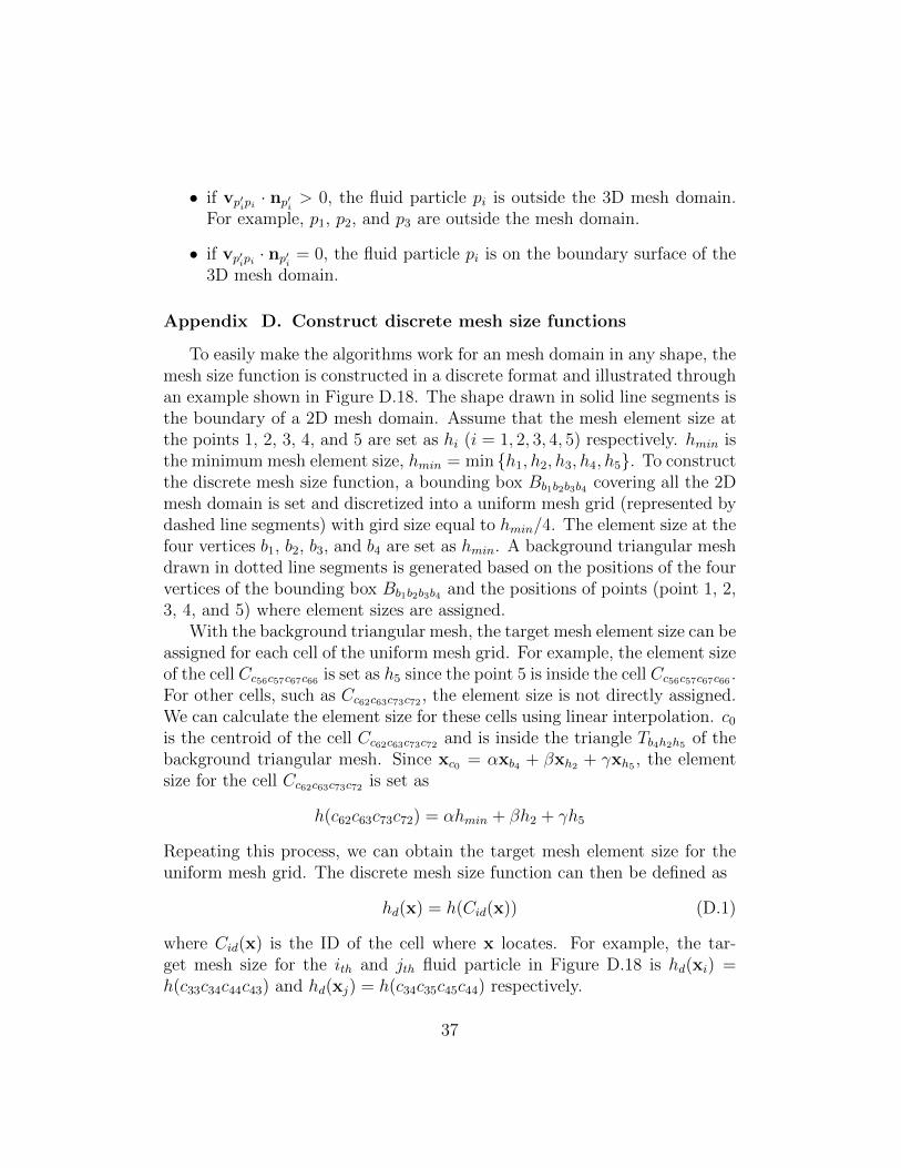
To easily make the algorithms work for an mesh domain in any shape, themesh size function is constructed in a discrete format and illustrated throughan example shown in Figure D.18. The shape drawn in solid line segments isthe boundary of a 2D mesh domain. Assume that the mesh element size atthe points 1, 2, 3, 4, and 5 are set as hi (i = 1, 2, 3, 4, 5) respectively. hmin isthe minimum mesh element size, hmin = min {h1, h2, h3, h4, h5}. To constructthe discrete mesh size function, a bounding box Bb1b2b3b4 covering all the 2Dmesh domain is set and discretized into a uniform mesh grid (represented bydashed line segments) with gird size equal to hmin/4. The element size at thefour vertices b1, b2, b3, and b4 are set as hmin. A background triangular meshdrawn in dotted line segments is generated based on the positions of the fourvertices of the bounding box Bb1b2b3b4 and the positions of points (point 1, 2,3, 4, and 5) where element sizes are assigned.
With the background triangular mesh, the target mesh element size can beassigned for each cell of the uniform mesh grid. For example, the element sizeof the cell Cc56c57c67c66 is set as h5 since the point 5 is inside the cell Cc56c57c67c66 .For other cells, such as Cc62c63c73c72 , the element size is not directly assigned.We can calculate the element size for these cells using linear interpolation. c0
is the centroid of the cell Cc62c63c73c72 and is inside the triangle Tb4h2h5 of thebackground triangular mesh. Since xc0 = αxb4 + βxh2 + γxh5 , the elementsize for the cell Cc62c63c73c72 is set as
h(c62c63c73c72) = αhmin + βh2 + γh5
Repeating this process, we can obtain the target mesh element size for theuniform mesh grid. The discrete mesh size function can then be defined as
hd(x) = h(Cid(x)) (D.1)
where Cid(x) is the ID of the cell where x locates. For example, the tar-get mesh size for the ith and jth fluid particle in Figure D.18 is hd(xi) =h(c33c34c44c43) and hd(xj) = h(c34c35c45c44) respectively.
37
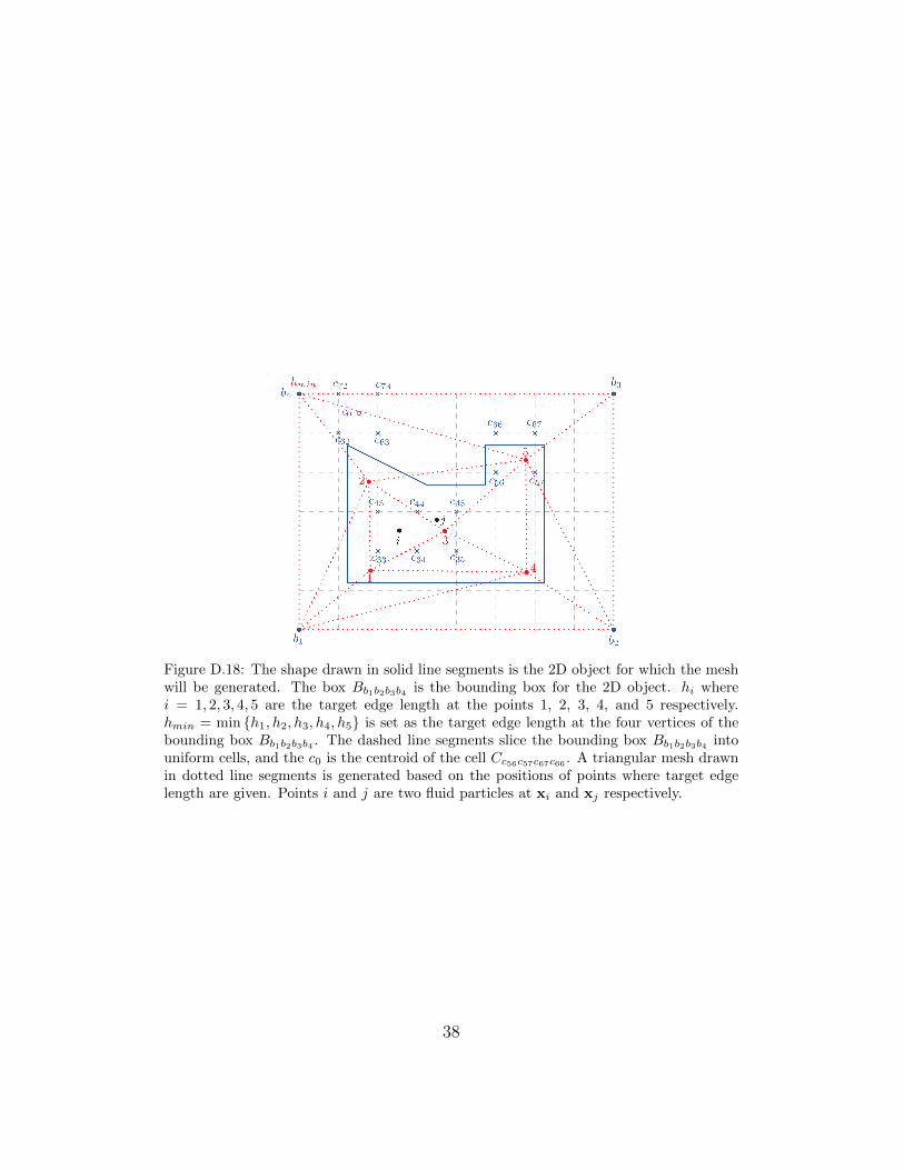
Figure D.18: The shape drawn in solid line segments is the 2D object for which the meshwill be generated. The box Bb1b2b3b4 is the bounding box for the 2D object. hi wherei = 1, 2, 3, 4, 5 are the target edge length at the points 1, 2, 3, 4, and 5 respectively.hmin = min {h1, h2, h3, h4, h5} is set as the target edge length at the four vertices of thebounding box Bb1b2b3b4 . The dashed line segments slice the bounding box Bb1b2b3b4 intouniform cells, and the c0 is the centroid of the cell Cc56c57c67c66 . A triangular mesh drawnin dotted line segments is generated based on the positions of points where target edgelength are given. Points i and j are two fluid particles at xi and xj respectively.
38