Flow Visualization around Generic Bridge Shapes using Particle Image Velocimetry

by Harold Bosch 1 and Kornel Kerenyi 2

1 Research Structural Engineer, Director of Aerodynamics Laboratory (HRDI-07), Federal Highway Administration, 6300 Georgetown Pike, McLean, Virginia 22101; PH (202) 493-3031; FAX (202) 493-3442; email: harold.bosch@fhwa.dot.gov 2 Hydraulic Research Engineer, GKY and Associates, Inc., 5411-E Backlick Road, Springfield, Virginia 22151; PH (703) 642-5080; FAX (703) 642-5367; email: kornel.kerenyi@fhwa.dot.gov

ABSTRACT This paper examines the flow field around generic bridge shape models using particle image velocimetry technique (PIV). Experiments were performed in a 2800 mm long and 450 mm wide flume. Plexi-glass models were used to avoid shadows and reflections in the light sheet. The PIV set-up used for these experiments was self-developed. The correlation algorithms were programmed in LabVIEW and IMAQ Vision. Nonlinear fit functions are used for calibration and image de-warping. A high-speed, high-resolution interline-transfer CCD digital camera that features a built in electronic shutter with exposure times as short as 127 microseconds is used for recording. Using a dual laser-head system designed to provide a highly stable green light source for PIV applications generated a light sheet. Detection and correction of false vectors and calculation of derived flow magnitudes are two features employed by the PIV method that enhance the quality of the delivered PIV vector maps. After the velocity flow fields are validated, standard differentiation schemes can be used to perform numerical vector field operations to compute streamlines and vorticity, even in the very complex flow patterns that occur around bridge decks. KEYWORDS: Generic Bridge Shapes, Particle Image Velocimetry, Bridge Engineering, Wind Engineering 1.0 INTRODUCTION

The particle image velocimetry technique (PIV) is an optical flow diagnostic based on the interaction of light refraction and scattering with non-homogeneous media. In the PIV method, the fluid motion is made visible by tracking the locations of small tracer particles at two instances of time. The particle displacement as a function of time is then used to infer the velocity flow field.

Adrian (1988) laid the initial groundwork for the PIV theory by describing the expectation value of the auto-correlation function for a double-exposure continuous PIV image. This description provided the framework for experimental design rules (Keane and Adrian 1990). PIV has developed toward the use of electronic cameras for direct recording of the particle images (Willert and Gharib, 1991). The theory was further extended by Westerweel (1993) to include digital PIV images and the estimation of the displacement at sub-pixel level. Westerweel (1997) summarizes the fundamental aspects of PIV signal analysis. The measurement principle is described in terms of linear system theory, in which the tracer particles are viewed as an observable pattern that is tied to the fluid. The observed tracer patterns at two subsequent instances are considered as the input and output of the system and the velocity field is inferred from the analysis of the input and output signals. The tracer pattern is then related to the observed (digital) image. The statistical description of the discrete PIV images is subsequently applied to evaluate the estimation of the particle-image displacement as a function of the spatial resolution (Raffel, Willert and Kompenhans, 1998). Research at the Federal Highway Administration (FHWA) Turner Fairbank Highway Research

Center (TFHRC) Hydraulics and Aerodynamics Laboratory has focused on using this technology for measuring instantaneous flow fields around bridge pier models. To date, research has focused on development of an in-house Particle Image Velocimetry system using LabVIEW and IMAQ Vision programming languages for post-processing and control of the camera and laser. A PXI compact PCI computer with a PXI 1422 IMAQ module as the frame grabber card is used in the system. A double-pulsed laser triggered with a high-resolution camera provides the light source. This technology accurately measures the velocity in complex situations, such as flow around bridge decks. The velocity measurements can be used to determine streamlines, vorticity, shear strain, vortex shedding frequencies, drag and lift forces that can threaten the structural stability of bridges. This paper shows the current status of the PIV system at the TFHRC Hydraulics and Aerodynamics Laboratory. 2.0 EXPERIMENTAL SET-UP The experimental set-up of a PIV system typically consists of several subsystems. In most applications tracer particles are added to the flow. These particles are illuminated in a plane of the flow at least twice within a short time interval. The light scattered by the particles is recorded either on a single frame or on a sequence of frames. The displacement of the particle images between the light pulses is determined through evaluation of the PIV recordings. 2.1 Flume The flume for the PIV set-up is 2800 mm long and 450 mm wide (Figure 1). The models in the flume are designed to investigate the flow around generic bridge shapes. The models are constructed from plexi-glass to avoid reflections. The upstream flow conditioning is achieved using filter mats and honeycomb flow straighteners. The sidewalls of the flume are made of glass, allowing excellent flow visibility. The flow discharge can be varied between 0 and 5 l/s. The flow depth used for these tests was 80

mm. An electromagnetic velocity probe measures the approach velocity. 2.2 Models A set of different models “generic bridge shapes” was studied for flow visualization. The models are simplified models of existing bridge decks excluding railing and other details (Figure 2). The model scale of the section models was designed to be 1 : 75 resulting in an average width of 130 mm and a height of 18.4 mm. All models were mounted vertically in the flume (model length = 102 mm). The angle of attack was varied between -15° and +15° using 5° increments. 2.3 Digital camera A Roper Scientific MEGAPLUS Model ES1.0 digital camera converts the light into an electrical charge. This model is designed for scientific and industrial applications. The camera is a stand-alone device that is connected through a 68-pin SCSI cable to the frame grabber card. PIV has a special demand on digital cameras. Therefore, a camera that operates under different modes is essential for use with the PIV system. Most important is the triggered double exposure mode that reduces exposure times for high-speed cases. The exposure is started through a trigger signal from the frame grabber card or through an external signal that can be supplied on the external trigger connector. An electronic shutter controls the exposure time that can be limited to 127µs. The spatial resolution is limited to 1008 (H) x 1018 (V) pixel which is implemented in a Charged Coupled Device (CCD) array. The dual channel output line, which has a data rate of 20 MHz, allows a maximum repetition rate of 30 fps and 15 fps in the triggered double exposure mode. For the laser, which must be synchronized with the image capture, an external strobe connector provides a trigger signal. 2.4 Light source To generate the light sheet a double-pulsed Solo PIV 120 laser was used. The Solo PIV 120 laser is a compact, dual laser-head system designed to provide a highly stable green light source for PIV

applications. The laser is ideally suited for fluid based PIV experiments, due to its small size that allows for flexibility in its installation. At the TFHRC Hydraulics Laboratory two laser heads with 1064 nm output wavelength are mounted on a single base plate. The beams generated by these laser heads are combined and then enter a second harmonic generator to produce green (532 nm) laser pulses. The output of the second harmonic generator impinges on dichroic mirrors that transmit the residual 1064 nm energy to metal absorbers and reflect the 532 nm green energy to the laser exit port. 2.5 Tracer (seeding) particles The choice of the right seeding material to scatter the light from the laser beams or the light sheet can be crucial to the quality of the acquired images. Numerous properties of the particle material are taken into consideration when selecting the appropriate seeding medium for a particular measurement task. Mean particle size is only one of the parameters. Other parameters of importance include the specific gravity, shape, surface characteristics and refractive index of the particles and the range of the size distribution. Silver-coated hollow glass spheres (S-HGS) are implemented in the flume at the TFHRC Hydraulics and Aerodynamics Laboratory. These borosilicate glass particles with a spherical shape and a smooth surface are intended primarily for liquid flow applications. A thin silver coating further increases reflectivity. 2.6 LabVIEW A LabVIEW programming system is used for image acquisition, control and post processing for the PIV system. LabVIEW programs are built on ‘Virtual Instruments’ (VI). A VI contains a front panel for the graphical user interaction, a block diagram for the logical processing (Figure 3), an icon for representing the VI and a connector pane for incoming and outgoing data. All nodes are connected through wires and have an input and an output. A node can only be executed when a wire presents data at the input. After executing, the data flows through the output to the next node. A node represents a control

structure, a sub VI or an indicator. In this manner the flow of data is controlled. 3.0 PIV RECORDING In order to handle the large amount of data generated by the PIV technique, sophisticated post-processing is required. The local displacement vector for the images of the tracer particles of the first and second frame is determined by statistical methods. 3.1 Raw Images and Frequency Filter Raw images can have extraneous noise introduced during the digitization process. To improve the image quality, a frequency filter is used to alter pixel values with respect to the periodicity and spatial distribution of the variations in light intensity in the image (Figure 4). Post-processing uses a high-pass frequency filter that attenuates or removes low frequencies present in the complex image. This filter suppresses information related to slow variations of light intensities in the spatial image. In this case, an inverse Fast Fourier Transform (FFT) used after a high-pass frequency filter produces an image in which overall patterns are sharpened and details are emphasized (NI IMAQ, 2000). 3.2 Cross-correlation PIV recordings are subdivided into interrogation areas, during evaluation. It is assumed that all particles within one interrogation area move homogeneously between two illuminations. The displacement of the particle images between the light pulses is evaluated by locally cross-correlating two frames of single exposures of the tracer ensemble (Figure 5). With both images I and I’ known, the aim is to estimate the displacement field. This is accomplished through use of the discrete cross-correlation function (1):

)()(II yj,xi'Ij,iIRK

Ki

L

Lj

++=∑∑−= −=

(1)

The correlation theorem which states that the cross-correlation of two functions is equivalent to a complex conjugate of their Fourier transforms (2) is used,

*'IIR ⋅⇔II (2) where I and *'I are the Fourier transforms of the functions I and I’, respectively (Figure 6). 4.0 RESULTS In many fluid dynamic applications the velocity information by itself is of secondary interest in the physical description. However, the velocity field obtained by PIV can be used to estimate other fluid attributes by means of differentiation or integration. Differentiation of the velocity field results in the velocity gradient tensor from which vorticity can be calculated. Integration of the velocity field results in the stream function and potential function. 4.1 Interpolating the vectors The correlation of the interrogation windows leads to discrete velocity vectors in the center of every interrogation area. To gain the velocity information for every pixel, bilinear interpolation is performed. Consider a point p inside one rectilinear cell (Figure 7). This cell has four corner points p0,0, p1,0, p0,1 and p1,1, , v00 ,vr 01,

r, v 10 ,r

and . The vector at p can be calculated using the values u and v and bilinearly interpolating the vectors at the corners using equation (3) (Joy, 1999).

11,vr

1,11,0

0,10,0

vuvvu-1vvuv-1vu-1v-1v

rr

rrr

+++=

)()()()(

(3)

In Figure 8 bilinear interpolation is applied to visualize the velocity flow field around the section models using a horizontal light sheet plane (Figure 1). 4.2 Integration The integration schemes are based on the

assumption that the integrand, that is the flow field, is two-dimensional as well as incompressible. In this case, potential theory relates the velocity field, U = (U (X,Y), V (X,Y)), to the stream function Ψ which can be integrated over the domain (X,Y plane) to:

∫∫ −=XY

dXVdYUΨ (4)

Figure 9 shows a two-dimensional stream function computed from equation (4) for PIV tests around the selected generic bridge shapes using a horizontal light sheet according to Figure 1. 4.3 Differentiation Since PIV provides the velocity vector field sampled on a two-dimensional evenly spaced grid, finite differencing has to be employed in the estimation of the spatial derivatives of the velocity gradient tensor. The PIV data, which provides the U and V velocity components, can only be differentiated in the X and Y directions. The terms of the deformation tensor that can be estimated with PIV are vorticity (5) and shear strain (6):

YU

XV

Z ∂∂−

∂∂=ω (5)

YU

XV

XY ∂∂+

∂∂=ε (6)

Only the vorticity component normal to the light sheet can be determined, along with the in-plane shearing and extensional strains. Figures 10 show the vorticity field estimate using a horizontal light sheet for the bridge deck models. 4.4 Vortex Shedding Frequencies The vorticity field estimate can be used to determine vortex-shedding frequencies. According to the kinematical relationship the vortex shedding frequency fo can be computed as follows

s

cVλ

=of (7)

In equation (7) Vc represents the mean convective velocity of a vortex between two marked vortices and λs corresponds to the distance between to marked vortices. As shown in figure 11 two vortices are marked (vortex A and B), λs is determined, then the time is recorded until vortex A reaches the end of λs so the mean convective velocity can be computed Vc. 5.0 CONCLUSIONS In contrast to techniques for the measurement of flow velocities employing probes such as pressure tubes or hot film wires, the PIV technique, being an optical technique, works nonintrusively. Hence, in contrast to standard methodologies, PIV eliminates the need for equipment that can be damaged by shocks in high-speed flows. In addition, PIV does not use probes or other measurement devices that interfere with velocity flows in boundary layers close to a wall. Overall, PIV is a more versatile technique, which allows one to record images of large parts of flow fields in a variety of applications and to extract the velocity information out of these images. This paper summarizes the development of a PIV system at the TFHRC Hydraulics and Aerodynamics Laboratory. The next step will include development of more advanced post-processing techniques, such as estimating pressure fields and extracting the third component of the velocity vector field (stereo techniques). In addition, this PIV technology will be deployed in a new demonstration wind tunnel to be installed in the Aerodynamics Laboratory within the next months. The biggest advantage of developing an in-house system is the flexibility to continually extend the PIV system. 6.0 REFERENCES Adrian, R., J., (1988), Statistical properties of particle image velocimetry measurements in turbulent flow, Laser Anemometry in Fluid

mechanics ed R. J. Adrian et al. (Lisbon: Instituto Superior Tecnico) pp. 115-29

Joy, K., I., (1999), Numerical Methods for Particle Tracing in Vector Fields, www.cs.ucdavis.edu/~ma/ECS177/particle_tracing.pdf

Keane, R., D. and Adrian, R., J., (1990), Meas. Sci. Technol. 1

NI IMAQ, (2000), IMAQ Vision Concepts Manual, National Instruments

Raffel, M., Willert, C., E., and Kompenhans, J., (1998), Particle Image Velocimetry – A Practical Guide, Springer-Verlag Berlin Heidelberg

Westerweel, J., (1993), Digital Particle Image Velocimetry – Theory and Application (Delft: Delft University Press)

Westerweel, J., (1997), Fundamentals of digital particle image velocimetry, Meas. Sci. Technol. 8, 1379-1392

Willert, C., E., and Gharib, M., (1991), Exp. Fluids 10 181

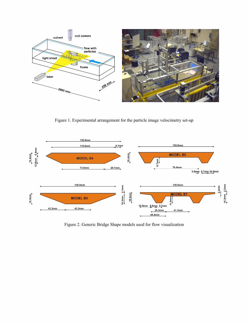
Figure 1. Experimental arrangement for the particle image velocimetry set-up

Figure 2. Generic Bridge Shape models used for flow visualization

Figure 3. Front panel and diagram panel of the PIV software in LabVIEW

Figure 4. Raw and frequency filtered images and LabVIEW block diagram

Figure 5. Two frames with interrogation areas and cross-correlation function RII for the two sub areas.

Figure 6. Implementation of cross-correlation using fast Fourier transforms

Figure 7. Vectors at the four corners of a cell and point p inside the cell of rectilinear area

Figure 8. Bilinear interpolated velocity flow field for the analyzed bridge deck shapes. Angle of attack =

15°.

Figure 9. Integrated two dimensional stream functions for the simplified bridge deck shapes. Angle of

attack = 15°.

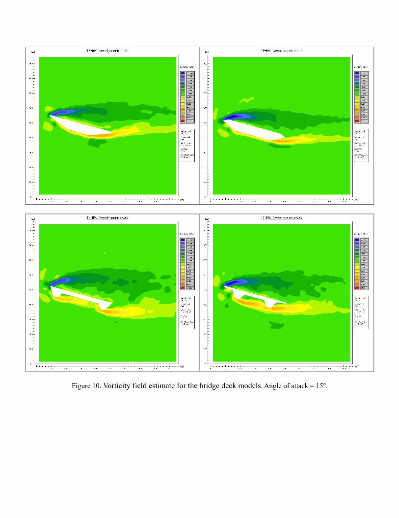
Figure 10. Vorticity field estimate for the bridge deck models. Angle of attack = 15°.

Figure 11. Using the kinematical relationship and vorticity field to determine the vortex-shedding frequencies. For λs = 5.5 cm and VC = 6.87 cm/s the vortex-shedding frequency fo = 1.25 Hz.