flow past a cylinder with a flexible splitter plate: a
TRANSCRIPT

HAL Id: hal-01018342https://hal.archives-ouvertes.fr/hal-01018342
Submitted on 4 Jul 2014
HAL is a multi-disciplinary open accessarchive for the deposit and dissemination of sci-entific research documents, whether they are pub-lished or not. The documents may come fromteaching and research institutions in France orabroad, or from public or private research centers.
L’archive ouverte pluridisciplinaire HAL, estdestinée au dépôt et à la diffusion de documentsscientifiques de niveau recherche, publiés ou non,émanant des établissements d’enseignement et derecherche français ou étrangers, des laboratoirespublics ou privés.
Distributed under a Creative Commons Attribution - NonCommercial - NoDerivatives| 4.0International License
Flow past a cylinder with a flexible splitter plate: Acomplementary experimental-numerical investigation
and a new FSI test case (FSI-PfS-1a)Guillaume de Nayer, Andreas Kalmbach, Michael Breuer, Stefan Sicklinger,
Roland Wüchner
To cite this version:Guillaume de Nayer, Andreas Kalmbach, Michael Breuer, Stefan Sicklinger, Roland Wüchner. Flowpast a cylinder with a flexible splitter plate: A complementary experimental-numerical investiga-tion and a new FSI test case (FSI-PfS-1a). Computers and Fluids, Elsevier, 2014, 99, pp.18-43.�10.1016/j.compfluid.2014.04.020�. �hal-01018342�

Flow past a cylinder with a flexible splitter plate: a complementary
experimental-numerical investigation and a new FSI test case
(FSI-PfS-1a)
G. De Nayera, A. Kalmbacha, M. Breuera,∗, S. Sicklingerb, R. Wuchnerb
aProfessur fur Stromungsmechanik, Helmut-Schmidt-Universitat Hamburg, D-22043 Hamburg, GermanybLehrstuhl fur Statik, Technische Universitat Munchen, D-80290 Munchen, Germany
Abstract
The objective of the present paper is to provide a challenging and well-defined validation testcase for fluid-structure interaction (FSI) in turbulent flow to close a gap in the literature. Thefollowing list of requirements are taken into account during the definition and setup phase.First, the test case should be geometrically simple which is realized by a classical cylinderflow configuration extended by a flexible structure attached to the backside of the cylinder.Second, clearly defined operating and boundary conditions are a must and put into practice bya constant inflow velocity and channel walls. The latter are also evaluated against a periodicsetup relying on a subset of the computational domain. Third, the material model shouldbe widely used. Although a rubber plate is chosen as the flexible structure, it is demon-strated by additional structural tests that a classical St. Venant-Kirchhoff material model issufficient to describe the material behavior appropriately. Fourth, the flow should be in theturbulent regime. Choosing water as the working fluid and a medium-size water channel,the resulting Reynolds number of Re = 30, 470 guarantees a sub-critical cylinder flow withtransition taking place in the separated shear layers. Fifth, the test case results should beunderpinned by a detailed validation process. For this purpose complementary numerical andexperimental investigations were carried out. Based on optical contactless measuring tech-niques (particle-image velocimetry and laser distance sensor) the phase-averaged flow field andthe structural deformations were determined. These data were compared with correspondingnumerical predictions relying on large-eddy simulations and a recently developed semi-implicitpredictor-corrector FSI coupling scheme. Both results were found to be in close agreementshowing a quasi-periodic oscillating flexible structure in the first swiveling FSI mode with acorresponding Strouhal number of about StFSI = 0.11.
Keywords: Fluid-structure interaction (FSI); FSI validation test case; FSI benchmark;turbulent reference experiment; particle-image velocimetry (PIV); coupled numericalsimulation; large-eddy simulation (LES); shell.
1. Introduction
A flexible structure exposed to a fluid flow is deformed and deflected owing to the fluid forcesacting on its surface. These displacements influence the flow field resulting in a couplingprocess between the fluid and the structure shortly denoted fluid-structure interaction (FSI).
∗Corresponding authorEmail address: [email protected] (M. Breuer)
1 INTRODUCTION 2
Due to its manifold forms of appearance it is a topic of major interest in many fields ofengineering. Based on enhanced numerical algorithms and increased computational resourcesnumerical simulations have become an important and valuable tool for solving this kind ofproblem within the last decade. Today FSI simulations complement additional experimentalinvestigations. A long-lasting vision of the computational engineer is to completely replaceor at least strongly reduce expensive experimental investigations in the foreseeable future.However, to attain this goal validated and thus reliable simulation tools are required.The long-term objective of the present research project is the coupled simulation of biglightweight structures such as thin membranes exposed to turbulent flows (outdoor tents,awnings...). To study these complex FSI problems, a multi-physics code framework was re-cently developed (Breuer et al., 2012). In order to assure reliable numerical simulations ofcomplex configurations, the whole FSI code needs to be validated at first on simpler test caseswith trusted reference data. In Breuer et al. (2012) the verification process of the code de-veloped is detailed. The computational fluid dynamics (CFD) and computational structuraldynamics (CSD) solvers were at first checked separately and then, the coupling algorithm wasconsidered in detail based on a laminar benchmark. A 3D turbulent example was also takeninto account to prove the applicability of the newly developed coupling scheme in the contextof large-eddy simulations (LES). However, owing to missing reference data a full validationwas not possible. The overall goal of the present paper is to present a turbulent FSI testcase supported by experimental data and numerical predictions based on the multi-physicscode developed. Thus, on the one hand the current FSI methodology involving LES and shellstructures undergoing large deformations is validated. On the other hand, a new turbulentFSI validation test case is defined based on detailed measurements and with specific insightsinto numerical flow simulations, computational structural analysis as well as coupling issues.Hence, the present study should provide a precisely described test case to the FSI communityfor the technically relevant case of turbulent flows interacting with flexible thin structures. Topropose a new FSI test case supported by experimental data a brief literature study of theavailable FSI test cases with simple flexible thin structures has to be done. These validationtest cases can be divided into two groups: the laminar and the turbulent cases. For the sakeof brevity complicated FSI cases are ignored in the following summary.As laminar, purely numerical FSI test cases one can cite the 2D and 3D modified cavity flowsof Wall (1999) and Mok (2001), taken as example in Forster et al. (2007): This is a modificationof the well-known lid-driven cavity CFD benchmark with a flexible membrane at the bottom.The CFD part of the FSI code can be validated at first with the classical lid-driven cavity flow.Then based on a simple modification assuming a flexible instead of a rigid bottom wall, theFSI coupling algorithm can be evaluated. This test is purely numerical and no experimentaldata are provided.From the very first, the hemodynamics research domain was interested in FSI to study bloodflow in flexible veins and arteries. Therefore, as 2D and 3D numerical laminar test cases themodel of a compliant vessel of Nobile (2001) and Formaggia et al. (2001) have to be cited. Thisunsteady test case is often used to validate FSI codes relying on shells, because of its simplicityand of the 3D structure deformations. Regarding other laminar benchmarks, there are manyFSI test cases with elastic plates: a very simple test case is the 2D numerical laminar test caseused by Gluck et al. (2001). A cantilever plate is transversely put into a flow. The solutionis stationary and the displacement is small. It is too simple to validate a FSI code, but veryuseful to debug and evaluate the coupling scheme. In Gluck et al. (2001) another test caseis presented: a L-shaped flexible body is located in a laminar flow and mounted headlong atthe bottom wall. This case is 3D and stationary, at least for moderate Reynolds numbers. It

1 INTRODUCTION 3
is useful for first 3D coupling tests, but no experimental data are provided. Balint and Lucey(2005) carried out a 2D cantilever plate in axial flow in order to describe human snoring causedby flutter of the soft palate. Two Reynolds numbers are tested with large deflections of theplate and numerical flow results are provided. More complicated is the 2D numerical laminarbenchmark of Wall and Ramm (1998), which was later modified by Hubner et al. (2004): Athin elastic cantilever plate is attached behind a rigid square cylinder. The geometry is simple,but the deformations of the structure are significant, which implies a good structure modelfor the great displacements expected and an appropriate remeshing or robust mesh movingprocedure for the CFD solver. Moreover, the artificial added-mass effect is strong. Therefore,it represents an appropriate benchmark to test the coupling method (Boyer et al., 2011).The well-known 2D numerical laminar benchmarks of Turek and Hron (2006) and Turek et al.(2010) developed in a collaborative research effort on FSI (Bungartz et al., 2010) have to becited here, too: An elastic cantilever plate is clamped behind a rigid circular cylinder. Threedifferent test cases, named FSI1, FSI2 and FSI3 are provided, complemented by additional self-contained CFD and CSD test cases to check both solvers independently. These test cases werealso used to validate the solvers applied in the present study (Breuer et al., 2012). The laminarbenchmarks proposed above are all purely numerical, i.e., a cross-comparison between differentnumerical results is possible, but no rigorous validation against experimental measurementscan be carried out.In order to close this gap, a nominally 2D laminar experimental case was provided by Gomesand Lienhart (2006, 2013) and Gomes (2011): A very thin metal sheet with an additionalweight at the end is attached behind a rotating circular cylinder and mounted inside a channelfilled with a mixture of polyglycol and water to reach a low Reynolds number in the laminarregime. Experimental data are provided for several inflow velocities and two different swivelingmotions could be identified depending on the inflow velocity. Owing to the thin metal sheetand the rear mass the accurate prediction of this case is demanding. A first comparisonbetween this laminar benchmark and numerical simulations can be found in Gomes et al.(2011): two configurations with different inflow velocities were taken into account. The FSIcode is composed of FASTEST-3D (see Section 4.1) for the CFD side and of FEAP (Taylor,2002) for the CSD side. The results show a very good agreement for the configuration with thehigher inflow velocity (second swiveling FSI mode). Nevertheless, differences were observed forthe low inflow velocity leading to the first swiveling FSI mode. Gomes et al. (2011) explainedthese deviations by the influence of the structural damping: in the high inflow velocity case therelevant frequency for the excitation process is the frequency of the coupled system (motion-induced excitation (MIE), see Naudascher and Rockwell (1994)). In the low inflow velocitycase, the relevant frequency for the excitation process is the first natural frequency of thepure structure surrounded by vacuum (instability-induced excitation (IIE), see Naudascherand Rockwell (1994)). Thus as argued by Gomes et al. (2011), for the first swiveling mode theFSI phenomenon is more sensitive to the structural damping, which was not considered in thenumerical model.The second category in the classification of FSI benchmarks presented here is composed of testcases based on turbulent flows involving 2D structures: In Gomes et al. (2010) a rigid plate witha single rotational degree of freedom was mounted into a water channel and experimentallystudied by particle-image velocimetry (PIV). This study also presents the first comparisonbetween experimental data and predicted results achieved by the present code for a turbulentFSI problem. As another turbulent experimental benchmark, the investigations of Gomes andLienhart (2010, 2013) and Gomes (2011) have to be cited: the same geometry as in Gomes andLienhart (2006) was used, but this time with water as the working fluid leading to much higher

2 DESCRIPTION OF THE VALIDATION TEST CASE 4
Reynolds numbers within the turbulent regime. The resulting FSI test case was found to bevery challenging from the numerical point of view. Indeed, the prediction of the deformationand motion of the very thin flexible structure requires two-dimensional finite-elements. Onthe other hand the discretization of the extra weight mounted at the end of the thin metalsheet calls for three-dimensional volume elements. Thus for a reasonable prediction of thistest case both element types have to be used concurrently and have to be coupled adequately.Additionally, the rotational degree of freedom of the front cylinder complicates the structuralsimulation and the grid adaptation of the flow prediction.Thus, in the present study a slightly different configuration is considered to provide in a firststep a less ambitious test case for the comparison between predictions and measurements focus-ing the investigations more to the turbulent flow regime and its coupling to a less problematicstructural model. For this purpose, a fixed cylinder with a thicker rubber tail and without arear mass is used. This should open the computation of the proposed benchmark case to abroader spectrum of codes and facilitates its adoption in the community. Strong emphasis isput on a precise description of the experimental measurements, a comprehensive discussion ofthe modeling in the numerical simulation (for the single field solutions as well as for the coupledproblem) and the processing of the respective data to guarantee a reliable reproduction of theproposed test case with various suitable methods.The paper is organized as follows: A detailed description of this new test case is given inSection 2. The measuring techniques used in the experiment are described in Section 3. Then,the numerical simulation methodology will be presented in Section 4 including a brief resumeof the theory of the multi-physics code. Afterwards the full numerical setup is explained.Due to cycle-to-cycle variations in the FSI phenomenon observed in the experiment and inthe simulation, the results have to be phase-averaged prior to a detailed comparison. Theprocess is described in Section 5. The experimental unsteady raw results are briefly presentedin Section 6. Finally, numerical and experimental phased-resolved results are compared anddiscussed in Section 7. All data available for comparison are specified in Section 8. For the sakeof clarity, the investigations on the material and on the structural model have been relegatedto Appendices at the end of the paper.
2. Description of the Validation Test Case
2.1. Description of the geometrical model and the test section
The proposed benchmark case, denoted FSI-PfS-1a, is derived from the turbulent benchmark ofGomes and Lienhart (2010, 2013). In their test case a very thin metal sheet with an additionalweight at the end was attached behind a rotating cylinder. The case was found to be verychallenging from the point of view of modeling and simulation. Therefore, the idea of thepresent paper is to propose a simpler FSI benchmark avoiding the aforementioned complicatedfeatures and being similar to the recently used FSI test case applied for LES studies (Breueret al., 2012), but supplemented by experimental data to compare with.FSI-PfS-1a consists of a flexible thin structure with a distinct thickness clamped behind afixed rigid non-rotating cylinder installed in a water channel (see Fig. 1). The cylinder hasa diameter D = 0.022 m. It is positioned in the middle of the experimental test section withHc = H/2 = 0.120 m (Hc/D ≈ 5.45), whereas the test section denotes a central part of theentire water channel (see Fig. 2). Its center is located at Lc = 0.077 m (Lc/D = 3.5) down-stream of the inflow section. The test section has a length of L = 0.338 m (L/D ≈ 15.36), aheight of H = 0.240 m (H/D ≈ 10.91) and a width W = 0.180 m (W/D ≈ 8.18). The blockingratio of the channel is about 9.2 %. The gravitational acceleration g points in x-direction (see

2 DESCRIPTION OF THE VALIDATION TEST CASE 5
Fig. 1), i.e. in the experimental setup this section of the water channel is turned 90 degrees.The deformable structure used in the experiment behind the cylinder has a length l = 0.060 m(l/D ≈ 2.72) and a width w = 0.177 m (w/D ≈ 8.05). Therefore, in the experiment there is asmall gap of about 1.5×10⁻³ m between the side of the deformable structure and both lateralchannel walls. The thickness of the rubber plate is h = 0.0021 m (h/D ≈ 0.09). This thicknessis an averaged value. The material is natural rubber and thus it is difficult to produce a per-fectly homogeneous 2 mm plate. The measurements show that the thickness is between 0.002and 0.0022 m. All parameters of the geometrical configuration of the FSI-PfS-1a benchmarkare summarized in Table 1.
WL
Hh
l
Hc
Lc
D
inflow zx
y
w
g
Figure 1: Sketch of the geometrical configuration of the validation test case within the test section.
Cylinder diameter D = 0.022 mCylinder center x-position Lc = 0.077 m Lc/D = 3.5Cylinder center y-position Hc= H/2 = 0.120 m Hc/D≈ 5.45Test section length L = 0.338 m L/D ≈ 15.36Test section height H = 0.240 m H/D ≈ 10.91Test section width W = 0.180 m W/D ≈ 8.18Deformable structure length l = 0.060 m l/D ≈ 2.72Deformable structure height h = 0.0021 m h/D ≈ 0.09Deformable structure width w = 0.177 m w/D ≈ 8.05
Table 1: Geometrical configuration of the FSI-PfS-1a validation test case.
2.2. Description of the water channel
In order to validate numerical FSI simulations based on reliable experimental data, the spe-cial research unit on FSI (Bungartz et al., 2010) designed and constructed a water channel(Gottingen type, see Fig. 2) for corresponding experiments with a special concern regardingcontrollable and precise boundary and working conditions (Gomes and Lienhart, 2006, 2010;Gomes, 2011). The channel (2.8 m × 1.3 m × 0.5 m, fluid volume of 0.9 m3) has a rectangular

2 DESCRIPTION OF THE VALIDATION TEST CASE 6
flow path and includes several rectifiers and straighteners to guarantee a uniform inflow intothe test section. To allow optical flow measurement systems like particle-image velocimetry,the test section is optically accessible on three sides. It possesses the same geometry as thetest section described in Section 2.1. The structure is fixed on the backplate of the test sectionand additionally fixed in the front glass plate. With a 24 kW axial pump a water inflow ofup to umax = 6 m/s is possible. To prevent asymmetries the gravity force is aligned with thex-axis in main flow direction.
channel
test section
motoraxial pump
1276
2775
straightener
240
338
180
z
x
y
x
Figure 2: Sketch of the flow channel (dimensions given in mm).
2.3. Flow parameters
Several preliminary tests were performed to find the best working conditions in terms of maxi-mum structure displacement, good reproducibility and measurable structure frequencies withinthe turbulent flow regime. Figure 3 depicts the measured extrema of the structure displace-ment versus the inlet velocity and Figure 4 gives the frequency and Strouhal number of the FSIphenomenon as a function of the inlet velocity. These data were achieved by measurementswith the laser distance sensor explained in Section 3.2. The entire diagrams are the result ofa measurement campaign in which the inflow velocity was consecutively increased from 0 to2.5 m/s. Four regions can be detected (see Fig. 3):
• uinflow ≤ 0.4 m/s: The deflections of the flexible structure are marginal resulting from fluidturbulence fluctuations. This is typical extraneously-induced excitation (EIE) mechanismas explained by Naudascher and Rockwell (1994).

2 DESCRIPTION OF THE VALIDATION TEST CASE 7
crossover1st swiveling mode
Vr1, 1
superposedhigher modes
inlet velocity [m/s]
Re
Uy/
D
0.0 0.5 1.0 1.5 2.0 2.5 3.0
0 10000 20000 30000 40000 50000 60000
-1.5
-1
-0.5
0
0.5
1
1.5
maximumminimum
Figure 3: Experimental displacements of the structure extremity versus the inlet velocity.
crossover1st swiveling mode
inlet velocity [m/s]
Re
FS
I fre
quen
cy [H
z]
FS
I Str
ouha
l num
ber
0.0 0.5 1.0 1.5 2.0 2.5 3.0
0 10000 20000 30000 40000 50000 60000
-5
0
5
10
15
20
25
-0.2
0
0.2
0.4
FSI frequency [Hz]FSI Strouhal number
Figure 4: Experimental measurements of the frequency and the corresponding Strouhal number ofthe FSI phenomenon versus the inlet velocity.
• 0.4 m/s < uinflow ≤ 1.65 m/s: The rubber plate deformations are quasi two-dimensionaland in the first swiveling mode. This region is dominated by an instability-induced exci-tation (IIE) (Naudascher and Rockwell, 1994). IIE is provoked by flow instability whichgives rise to flow fluctuations if a specific flow velocity is reached. These fluctuationsand the resulting forces become well correlated and their frequency is close to a nat-ural frequency of the flexible structure (lock-in phenomenon). In this case oscillationswith large amplitudes are expected. Here, the amplitudes increase until the maximumis reached at uinflow ≈ 1.54, which corresponds to the reduced velocity VrIIE1,1 ≈ 5.71. The
reduced velocity for IIE is defined as follows: VrIIEN,n = uinflow/(fND) ≈ 1/(n St). fN is anatural frequency of the flexible structure and St the Strouhal number defined with thevortex-shedding frequency around the undeformed body. The natural frequencies are de-termined by a modal analysis: The first frequency of the rubber plate f1 is found at about

2 DESCRIPTION OF THE VALIDATION TEST CASE 8
12.3 Hz and corresponds to the first swiveling mode dominant in the FSI phenomenon.St is about 0.175 as specified in Section 7.
• 1.65 m/s < uinflow ≤ 2.33 m/s: In this range the structural deflections are chaotic andthree-dimensional. This is a crossover phase. The frequency of the FSI phenomenonincreases until the first natural frequency of the rubber plate. Beyond this value it isdifficult to measure the FSI frequency because of the chaotic movement.
• 2.33 m/s < uinflow: The deformations observed are three-dimensional and several modesare superposed.
At an inflow velocity of uinflow = 1.385 m/s the displacements are symmetrical, reasonablylarge and well reproducible. Based on the inflow velocity chosen and the cylinder diameter theReynolds number of the experiment is equal to Re = 30, 470. Regarding the flow around thefront cylinder, at this inflow velocity the flow is in the sub-critical regime. That means theboundary layers are still laminar, but transition to turbulence takes place in the free shear layersevolving from the separated boundary layers behind the apex of the cylinder. Transition toturbulence means that from that point onwards the flow is three-dimensional and chaotic, andconsists of a variety of different length and time scales. The low-frequency components of theturbulent flow dominate the coupled FSI problem, whereas the high-frequency contributionsare visible in the fluid forces but are filtered out by the flexible structure. That is the reasonwhy the signals for the deflections show the quasi-periodic signals without high-frequencyfluctuations as will be shown below in Fig. 11.Except the boundary layers at the section walls the inflow was found to be nearly uniform iny- and z-direction (see Fig. 5). The time-averaged velocity components u and v are measuredwith two-component laser-Doppler velocimetry (LDV) along the y-axis in the middle of themeasuring section at x/D = 4.18 and z/D = 0. It can be assumed that the time-averagedvelocity component w shows a similar velocity profile as v. Furthermore, a low inflow tur-
bulence level of Tuinflow =
√
13
(
u′2 + v′2 + w′2
)
/uinflow = 0.02 is measured. All experiments
were performed with water under standard conditions at T = 20◦ C. The flow parameters aresummarized in Table 2.
inflow
inflow
Figure 5: Profiles of the time-averaged streamwise and normal velocity as well as the turbulencelevel at the inflow section of the water channel for the y-direction.

2 DESCRIPTION OF THE VALIDATION TEST CASE 9
Inflow velocity uinflow= 1.385 m/sFlow density ρf = 1000 kg/m3
Flow dynamic viscosity µf = 1.0×10⁻³ Pa s
Table 2: Flow parameters of the FSI-PfS-1a validation test case.
2.4. Choice of structural models and material parameters
Rubber materials are widely used in many different applications, due to, e.g., their isotropicmechanical behavior, their wide range of usable elastic deformations and their adaptabilityto different needs. Depending on the specific application, the suitable description of the me-chanical behavior must be realized by a more or less complex material model such as Ogden,Neo-Hooke, Mooney-Rivlin or Varga (Holzapfel, 2000). For the present FSI benchmark, thematerial and dimensions of the deformable structure should be selected in such a way that itis rather easy to excite the structure with only moderate fluid forces in the experiment (i.e., itshould not be too stiff) and it should undergo only reversible, i.e. elastic, deformations in therange of interest. Moreover, to enable the computation of this test case by many other groups,the structural setup should be simple in order to be described by as few parameters as possibleand the structural analysis should be feasible with even less sophisticated material laws like,e.g., St. Venant-Kirchhoff. Another issue is the wish to keep the structural modeling open toeither solid or shell finite element formulations which makes it necessary to avoid an excessivelythin structure to guarantee the desired flexibility. As a consequence of all these requirements,a custom-made flexible and isotropic rubber material with a reasonable thickness, produced bythe company Draftex Automotive GmbH, is applied and its material parameters are presentedbelow. For understanding the behavior of the rubber used for the structural model and toverify the characteristic parameters for the structural simulations, pure structural test caseswere defined and performed in the laboratory (See Appendix A).Although the material shows a strong non-linear elastic behavior for large strains, the appli-cation of a linear elastic constitutive law is favored, to enable the reproduction of this FSIbenchmark by a variety of different computational analysis codes without the need of complexmaterial laws. This assumption can be justified by the observation that in the FSI test case,a formulation for large deformations but small strains is applicable. Hence, the identificationof the material parameters is done on the basis of the moderate strain expected and the St.Venant-Kirchhoff constitutive law is chosen as the simplest hyper-elastic material model.
The density of the rubber material can be determined to be ρrubber plate = 1360 kg/m3 for athickness of the plate h = 0.0021 m. This permits the accurate modeling of inertia effects ofthe structure and thus dynamic test cases can be used to calibrate the material constants. Forthe chosen material model there are only two parameters to be defined: The Young’s modulusE and the Poisson’s ratio ν. In order to avoid complications in the needed element technologydue to incompressibility, the material was realized to have a Poisson’s ratio which reasonablydiffers from 0.5. Material tests of the manufacturer indicate that the Young’s modulus isE = 16 MPa and the Poisson’s ratio is ν = 0.48. The material parameters are summarized inTable 3.To numerically validate the decision on structural models and to check the material parameterssimulations are carried out with the reference software Abaqus1 on the pure structural test cases
1http://www.3ds.com/products/simulia/portfolio/abaqus/overview

3 MEASURING TECHNIQUES FOR THE EXPERIMENTAL INVESTIGATIONS 10
Flexible structure density ρrubber plate = 1360 kg/m3
Young’s modulus E = 16 MPaPoisson’s ratio ν = 0.48
Table 3: Structural parameters of the FSI-PfS-1a flexible structure.
described in Appendix A. The results are presented in Appendix B.
3. Measuring Techniques for the Experimental Investigations
Experimental FSI investigations need to contain fluid and structure measurements for a fulldescription of the coupling process. Under certain conditions, the same technique for bothdisciplines can be used. The measurements performed by Gomes and Lienhart (2006, 2010,2013) used the same camera system for the simultaneous acquisition of the velocity fields andthe structural deflections. This procedure works well for FSI cases involving laminar flows and2D structure deflections. In the present case the structure deforms slightly three-dimensionalwith increased cycle-to-cycle variations caused by turbulent variations in the flow. The ap-plied measuring techniques, especially for the structural side, have to deal with those changedconditions especially the formation of shades. Furthermore, certain spatial and temporal res-olutions as well as low measurement errors are requested. Due to the different deformationbehavior a single camera setup for the structural measurements like in Gomes and Lienhart(2006, 2010, 2013) used was not practicable. Therefore, the velocity fields were captured by a2D particle-image velocimetry (PIV) setup and the structural deflections were measured witha laser triangulation technique. Both devices are presented in the next sections.
3.1. Particle-image velocimetry
A classic particle-image velocimetry (Adrian, 1991) setup depicted in Fig. 6 consists of a singlecamera obtaining two components of the fluid velocity on a planar surface illuminated by alaser light sheet. Particles introduced into the fluid are following the flow and reflecting thelight during the passage of the light sheet. By taking two reflection fields in a short timeinterval ∆t, the most-likely displacements of several particle groups on an equidistant gridare estimated by a cross-correlation technique or a particle-tracking algorithm. Based on aprecise preliminary calibration, the displacements obtained and the time interval ∆t chosenthe velocity field can be calculated. To prevent shadows behind the flexible structure a secondlight sheet was used to illuminate the opposite side of the test section.The phased-resolved PIV-measurements (PR-PIV) were carried out with a 4 Mega-pixel camera(TSI Powerview 4MP, charge-coupled device (CCD) chip) and a pulsed dual-head Neodym:YAGlaser (Litron NanoPIV 200) with an energy of 200 mJ per laser pulse. The high energy of thelaser allowed to use silver-coated hollow glass spheres (SHGS) with an average diameter ofdavg,SHGS = 10µm and a density of ρSHGS = 1400 kg/m3 as tracer particles. To prove the fol-lowing behavior of these particles the Stokes number Sk and the particle sedimentation velocityuSHGS is calculated as follows:
SkSHGS =τp,SHGS
τf,SHGS
=ρSHGS d2avg,SHGS
18 µf
uinflow
davg,SHGS
= 1.08 ,
uSHGS =d2avg,SHGS g (ρSHGS − ρf )
18 µf
= 2.18×10⁻⁵ m/s .

3 MEASURING TECHNIQUES FOR THE EXPERIMENTAL INVESTIGATIONS 11
CCD camera
double-pulsed laser lenses
flow with reflecting particlesImage 1
Image 2
cross-correlation ofdisplacements
velocity field
Δ t
around the flexible structure
x
y
z
Figure 6: Measuring principle of a two-component PIV setup for the flow around the flexible struc-ture.
With this Stokes number and a particle sedimentation velocity which is much lower than theexpected velocities in the experiments, an eminent following behavior is approved. The cameratakes 12 bit pictures with a frequency of about 7.0 Hz and a resolution of 1695 × 1211 px withrespect to the rectangular size of the test section. For one phase-resolved position (described inSection 5) 60 to 80 measurements are taken. Preliminary studies with more and fewer measure-ments showed that this number of measurements represent a good compromise between accu-racy and effort. The grid has a size of 150 × 138 cells and was calibrated with an average factorof 126µm/px, covering a planar flow field of x/D ≈ −2.36 to 7.26 and y/D ≈ −3.47 to 3.47 inthe middle of the test section at z/D ≈ 0. The time between the frame-straddled laser pulseswas set to ∆t = 200µs. Laser and camera were controlled by a TSI synchronizer (TSI 610035)with 1 ns resolution. The processing of the phase-resolved fluid velocity fields involving thestructure deflections is described in Section 5.
3.2. Laser distance sensor
Non-contact structural measurements are often based on laser distance techniques. In thepresent benchmark case the flexible structure shows an oscillating frequency of about 7.1 Hz.With the requirement to perform more than 100 measurements per period, a time-resolvedsystem was needed. Therefore, a laser triangulation was chosen because of the known geomet-ric dependencies, the high data rates, the small measurement range and the resulting higheraccuracy in comparison with other techniques such as laser phase-shifting or laser interferom-etry. The laser triangulation uses a laser beam which is focused onto the object. A CCD-chiplocated near the laser output detects the reflected light on the object surface. If the distance ofthe object from the sensor changes, also the angle changes and thus the position of its image onthe CCD-chip. From this change in position the distance to the object is calculated by simpletrigonometric functions and an internal length calibration adjusted to the applied measurementrange. To study simultaneously more than one point on the structure, a multiple-point trian-gulation sensor was applied (Micro-Epsilon scanControl 2750, see Fig. 7). This sensor uses amatrix of CCD chips to detect the displacements on up to 640 points along a laser line reflectedon the surface of the structure with a data rate of 800 profiles per second. The laser line waspositioned in a horizontal (x/D ≈ 2.82, see Fig. 7(a)) and in a vertical alignment(z/D ≈ 0, seeFig. 7(b)) and has an accuracy of 40µm. Due to the different refraction indices of air, glassand water a custom calibration was performed to take the modified optical behavior of the

4 NUMERICAL SIMULATION METHODOLOGY 12
emitted laser beams into account.
b) multiple point sensor - xy-plane
laser light sheet
rigid cylinder with flexible structure
triangulation sensor
scattered light
x
y
z
a) multiple point sensor - yz-plane
x
y
z
Figure 7: Setup and alignment of multiple-point laser sensor on the flexible structure in a) z-directionand b) x-direction.
4. Numerical Simulation Methodology
The applied numerical method relies on an efficient partitioned coupling scheme developedfor dynamic fluid-structure interaction problems in turbulent flows (Breuer et al., 2012). Thefluid flow is predicted by an eddy-resolving scheme, i.e., the large-eddy simulation technique.FSI problems very often encounter instantaneous non-equilibrium flows with large-scale flowstructures such as separation, reattachment and vortex shedding. For this kind of flows theLES technique is obviously the best choice (Breuer, 2002). Based on a semi-implicit scheme theLES code is coupled with a code especially suited for the prediction of shells and membranes.Thus an appropriate tool for the time-resolved prediction of instantaneous turbulent flowsaround light, thin-walled structures results. Since all details of this methodology were recentlypublished in Breuer et al. (2012), in the following only a brief description is provided.
4.1. Computational fluid dynamics (CFD)
In the present methodology the temporally varying domain within a FSI application is takeninto account by the Arbitrary Lagrangian-Eulerian (ALE) formulation. The application ofthe ALE method is limited to FSI cases with mild or moderate deformations of the structure.For extreme deflections other techniques such as the immersed boundary method or oversetgrids should be applied. However, since in the current test case this restriction is satisfiedand the ALE method allows to adequately resolve the thin boundary layers on the structureusing curvilinear body-fitted grids without artificial boundary conditions, it is favored for thepresent application.The extra fluxes appearing in the filtered Navier-Stokes equations are consistently determinedby the space conservation law (SCL) (Demirdzic and Peric, 1988, 1990; Lesoinne and Farhat,1996). For this purpose the in-house code FASTEST-3D (Durst and Schafer, 1996; Durst et al.,1996) relying on a finite-volume scheme is used. The discretization on a block-structured body-fitted grid is second-order accurate in space.A predictor-corrector scheme (projection method) of second-order accuracy forms the kernel ofthe fluid solver. In the predictor step an explicit Runge-Kutta scheme advances the momentumequation in time. In the following corrector step the mass conservation equation is fulfilled by

4 NUMERICAL SIMULATION METHODOLOGY 13
solving a Poisson equation for the pressure-correction. The corrector step is repeated until apredefined convergence criterion is reached.In LES the large scales are resolved directly, whereas the non-resolvable small scales have to betaken into account by a subgrid-scale model. Here, the well-known Smagorinsky (1963) modelis applied. A Van Driest damping function ensures a reduction of the subgrid length near solidwalls. Owing to minor influences of the subgrid-scale model at the moderate Reynolds numberconsidered in this study, a dynamic procedure to determine the Smagorinsky parameter wasomitted and instead a well established standard constant Cs = 0.1 is used.
4.2. Computational structural dynamics (CSD)
The dynamic equilibrium of the structure is described by the momentum equation given ina Lagrangian frame of reference. Large deformations, where geometrical non-linearities arenot negligible, are allowed (Hojjat et al., 2010). According to the preliminary considerationsdescribed in Section 2.4, a total Lagrangian formulation in terms of the second Piola-Kirchhoffstress tensor and the Green-Lagrange strain tensor which are linked by the St. Venant-Kirchhoffmaterial law is used in the present study. The investigations within this paper were donewith the in-house code Carat++ (Fischer et al., 2010; Bletzinger et al., 2006), developedwith an emphasis on the prediction of shell or membrane behavior. Carat++ is based onseveral finite-element types and advanced solution strategies for form finding and non-lineardynamic problems (Wuchner and Bletzinger, 2005; Wuchner et al., 2007; Bletzinger et al.,2005; Dieringer et al., 2012). For the dynamic analysis, different time-integration schemes areavailable, e.g., the implicit generalized-α method (Chung and Hulbert, 1993). In the modelingof thin-walled structures, membrane or shell elements are applied. The deformable solid ismodeled with a 7-parameter shell element. Furthermore, special care is given to prevent lockingphenomena by applying the well-known Assumed Natural Strain (ANS) (Hughes and Tezduyar,1981; Park and Stanley, 1986) and Enhanced Assumed Strain (EAS) methods (Bischoff et al.,2004).Both, shell and membrane elements reflect geometrically reduced structural models with atwo-dimensional representation of the mid-surface which can describe the three-dimensionalphysical properties by introducing mechanical assumptions for the thickness direction. Dueto this reduced model additional operations are required to transfer information between thetwo-dimensional structure and the three-dimensional fluid model. Thus in the case of shells,the surface of the interface is found by moving the two-dimensional surface of the structure halfof the thickness normal to the surface on both sides and the closing of the volume (Bletzingeret al., 2006). On these two moved surfaces the exchange of data is performed consistently withrespect to the shell theory (Hojjat et al., 2010).
4.3. Coupling algorithm
To preserve the advantages of the highly adapted CSD and CFD codes and to realize an effectivecoupling algorithm, a partitioned but nevertheless strong coupling approach is chosen. Thescheme involves an explicit solution of the non-linear terms in the Navier-Stokes equations andan implicit coupling between the computation of the pressure field and the displacements ofthe structure. Thus small time steps typically required for LES to resolve the turbulent flowfield are taken into account in the coupling scheme relying on this explicit predictor-correctorscheme. Since all details are provided in Breuer et al. (2012), only a few issues forming thekernel of the fluid solver are provided here.For a flexible structure in water, the added-mass effect by the surrounding fluid plays a domi-nant role. In this situation a strong coupling scheme taking the tight interaction between the

4 NUMERICAL SIMULATION METHODOLOGY 14
fluid and the structure into account, is indispensable. In the coupling scheme developed inBreuer et al. (2012) this issue is taken into account by a FSI-subiteration loop which avoidsinstabilities due to the added-mass effect known from loose coupling schemes and maintainsthe explicit character of the time-stepping scheme beneficial for LES.At the beginning of a time step a prediction of the structural displacement is carried out bya first-order extrapolation to accelerate the convergence. A second-order prediction is notapplied, since it was observed that it does not improve the convergence for the current smalltime-step size.Based on the velocity and pressure fields from the corrector step, the fluid forces resulting fromthe pressure and the viscous shear stresses at the interface between the fluid and the structureare computed. These forces are transferred by a grid-to-grid data interpolation to the CSDcode Carat++ using a conservative interpolation scheme (Farhat et al., 1998) implemented inthe coupling interface CoMA (Gallinger et al., 2009). The conservative interpolation of theforces ensures that the load resultants on both grids are exactly the same. This advantage isaccompanied by the drawback that in case of a coarse source grid (CFD) and very fine targetgrid (CSD), the loads are distributed in a non-physical way. For the present and most otherFSI applications this is however not the case, since the grid used for LES is much finer thanthe CSD grid.Using the fluid forces provided via CoMA, Carat++ determines the stresses in the structureand the resulting displacements of the structure. This response of the structure is transferredback to the fluid solver via CoMA applying a bilinear interpolation which is a consistent schemefor four-node elements with bilinear shape functions.The CSD prediction determines displacements at the moving boundaries of the computationaldomain for the fluid flow. The task is to adapt at each FSI-subiteration the grid of theinner computational domain based on these displacements at the interface. For moderatedeformations algebraic methods are found to be a good compromise since they are extremelyfast and deliver reasonable grid point distributions maintaining the required high grid quality.Thus, the grid adjustment is performed based on a transfinite interpolation (Thompson et al.,1985). It consists of three shear transformations plus a tensor-product transformation.The code coupling tool CoMA is based on the Message-Passing-Interface (MPI) and thusruns in parallel to the fluid and structure solver. The communication in-between the codesis performed via standard MPI commands. Since the parallelization in FASTEST-3D andCarat++ also relies on MPI, a hierarchical parallelization strategy with different levels ofparallelism is achieved.For more details about this semi-implicit coupling scheme, we refer to Breuer et al. (2012).
4.4. Numerical setup
4.4.1. Grids
CFD prediction.For the CFD prediction of the flow two different block-structured grids either for a subset ofthe entire channel (w′/l = 1) or for the full channel but without the gap between the flexiblestructure and the side walls (w/l = 2.95) are used (see Fig. 8). In the first case the entiregrid consists of about 13.5 million control volumes (CVs), whereas 72 equidistant CVs areapplied in the spanwise direction. For the full geometry the grid possesses about 22.5 millionCVs. In this case starting close to both channel walls the grid is stretched geometrically with astretching factor 1.1 applying in total 120 CVs with the first cell center positioned at a distanceof ∆z/D = 1.7×10⁻².

4 NUMERICAL SIMULATION METHODOLOGY 15
inflow zx
y
subset case
full case
Figure 8: Differences between the full and the subset case.
The gap between the elastic structure and the walls is not taken into account in the numericalmodel and thus the width of the channel is set to w instead of W . Two main reasons areresponsible for this simplification. If the gap would be considered in the simulation, theboundary layers of the channel walls had to be fully resolved, which is too costly. Moreover,the cells in this gap would be subjected to heavy distortions during the FSI simulation, whichwould massively complicate the purpose of grid adaptation during the movement of the flexiblestructure close to the side walls and may even lead to convergence problems of the coupledsolver.
L
H
LC
Figure 9: x-y cross-section of the grids used for the simulation with 187,500 cells (Note that onlyevery fourth grid line in each direction is displayed here).
In the x-y cross-section both grids are identical (see Fig. 9). Since only every fourth grid lineof the mesh is shown in Fig. 9, the angles between grid lines and the transitions between theblocks appear to be worse than in the original grid. The numerical domain has a length of L.Since the inflow side is rounded in order to use a C-grid, the computational domain in frontof the cylinder is slightly larger than in the test section depicted in Fig. 1. The grid pointsare clustered towards the rigid cylinder and the flexible structure using a stretching function

4 NUMERICAL SIMULATION METHODOLOGY 16
according to a geometric series. The stretching factors are kept below 1.1 with the first cellcenter located at a distance of ∆y/D = 9×10⁻⁴ from the flexible structure. Based on the wallshear stresses on the flexible structure the average y+ values are predicted to be below 0.8,mostly even below 0.5. Thus, the viscous sublayer on the elastic structure and the cylinder isadequately resolved. Since the boundary layers at the upper and lower channel walls are notconsidered, no grid clustering is required here.
CSD prediction.Motivated by the fact that in the case of LES frequently a domain modeling based on periodicboundary conditions at the lateral walls is used to reduce the CPU-time requirements, thisspecial approach was also investigated for the FSI test case. The detailed discussion of this spe-cific boundary modeling for the spanwise direction is given in Section 4.4.2. As a consequence,there are two different structure meshes used: For the CSD prediction of the case with a subsetof the full channel the elastic structure is resolved by the use of 10×10 quadrilateral four-nodeshell elements. For the case discretizing the entire channel, 10 quadrilateral four-node shellelements are used in the main flow direction and 30 in the spanwise direction. These choices arederived from a grid independency study based on a representative pure structure simulationtest case with a very similar deformation pattern. This allows to avoid the high computationaloverhead of fully coupled FSI simulations. The investigations are presented in Appendix C.The finite elements for the structure are 7-parameter shell elements with 6 degrees of free-dom per node (Buchter and Ramm, 1992; Buchter et al., 1994; Bischoff and Ramm, 2000).The specific degrees of freedom are the three deformations of the mid-surface and the threecomponents of the difference vector of the shell director. Special treatments for the thicknessstretch are included to avoid the undesirable effect which is called thickness locking (Bischoffand Ramm, 1997). For the present test cases the ANS method is not activated and the EASmethod is used according to the recommendations in Bischoff et al. (2004) and Bischoff (1999),to have an effective counter-measure against transverse shear-, membrane-, in-plane shear andthickness locking. For a detailed derivation of the element, an in-depth discussion of valid shellformulations and locking phenomena in shell element analysis, the reader is referred to thesetwo studies. The shell elements used are formulated for large deformations, i.e., geometricallynon-linear analysis. In the given benchmark scenario, the ratio of the thickness and the lengthof the thin structure, h/l = 0.035, is smaller than 1/10. So even a 5-parameter shell using theReissner-Mindlin kinematics (Reissner, 1945; Mindlin, 1951) would be valid. The 7-parametertheory yields higher accuracy for the representation of through-the-thickness effects and is forthe structure considered fully comparable to a solid model.
4.4.2. Boundary conditions
CFD prediction.On the CFD side no-slip boundary conditions are applied at the rigid front cylinder and atthe flexible structure. Since the resolution of the boundary layers at the channel walls wouldrequire the bulk of the CPU-time, the upper and lower channel walls are assumed to be slipwalls. Thus the blocking effect of the walls is maintained without taking the boundary layersinto account. At the inlet a constant streamwise velocity is set as inflow condition withoutadding any perturbations. The choice of zero turbulence level is based on the consideration thatsuch small perturbations imposed at the inlet will generally not reach the cylinder due to thecoarseness of the grid at the outer boundaries. Therefore, all inflow fluctuations will be highlydamped. However, since the flow is assumed to be sub-critical, this disregard is insignificant.At the outlet a convective outflow boundary condition is favored allowing vortices to leave the

4 NUMERICAL SIMULATION METHODOLOGY 17
integration domain without significant disturbances (Breuer, 2002). The convection velocity isset to uinflow.As mentioned above two different cases are considered (see Fig. 8). In order to save CPU-time in the first case only a subset of the entire spanwise extension of the channel is takeninto account. Thus the computational domain has a width of w′/l = 1 in z-direction and theflexible structure is a square in the x-z-plane. In this case a reasonable approximation alreadyapplied in Breuer et al. (2012) is to apply periodic boundary conditions in spanwise directionfor both disciplines. For LES predictions periodic boundary conditions represent an oftenused measure in order to avoid the formulation of appropriate inflow and outflow boundaryconditions. The approximation is valid as long as the turbulent flow is homogeneous in thespecific direction and the width of the domain is sufficiently large. The latter can be provenby predicting two-point correlations, which have to drop towards zero within the half-width ofthe domain. The impact of periodic boundary conditions on the CSD predictions are discussedbelow.For the full case with w/l = 2.95 periodic boundary conditions can no longer be used. Instead,for the fluid flow similar to the upper and lower walls also for the lateral boundaries slipwalls are assumed since the full resolution of the boundary layers would be again too costly.Furthermore, the assumption of slip walls is consistent with the disregard of the small gapbetween the flexible structure and the side walls discussed above.
CSD prediction.On the CSD side, the flexible shell is loaded on the top and bottom surface by the fluid forces,which are transferred from the fluid mesh to the structure mesh. These Neumann boundaryconditions for the structure reflect the coupling conditions. Concerning the Dirichlet boundaryconditions, the four edges need appropriate support modeling: on the upstream side at therigid cylinder a clamped support is realized and all degrees of freedom are equal to zero. Onthe opposite downstream trailing-edge side, the rubber plate is free to move and all nodes havethe full set of six degrees of freedom. The edges which are aligned to the main flow directionneed different boundary condition modeling, depending on whether the subset or the full caseis computed:For the subset case due to the fluid-motivated periodic boundary conditions, periodicity forthe structure is correspondingly assumed for consistency reasons. As it turns out later inSection 7.1.1, this assumption seems to hold for this specific configuration and its deformationpattern which has strong similarity with an oscillation in the first eigenmode of the shell.Hence, this modeling approach may be used for the efficient processing of parameter studies,e.g., to evaluate the sensitivity of the FSI simulations with respect to slight variations in modelparameters shown in Section 7.1.2. For this special type of support modeling, there are alwaystwo structure nodes on the lateral sides (one in a plane z = −w/2 and its twin in the other planez = +w/2) which have the same load. These two nodes must have the same displacements inx- and y-direction and their rotations have to be identical. Moreover, the periodic boundaryconditions imply that the z-displacement of the nodes on the sides are forced to be zero.For the full case the presence of the walls in connection with the small gap implies that there isin fact no constraining effect on the structure, as long as no contact between the rubber plateand the wall takes place. Out of precise observations in the lab, the possibility of contact maybe disregarded. In principle, this configuration would lead to free-edge conditions like at thetrailing edge. However, the simulation of the fluid with a moving mesh needs a well-definedmesh situation at the side walls which made it necessary to tightly connect the structure meshto the walls (the detailed representation of the side edges within the fluid mesh is discarded due

5 GENERATION OF PHASE-RESOLVED DATA 18
to computational costs and the resulting deformation sensitivity of the mesh in these regions).Also the displacement in z-direction of the structure nodes at the lateral boundaries is forcedto be zero.
4.4.3. Coupling conditions
For the turbulent flow a time-step size of ∆tf = 2×10⁻⁵ s (∆t∗f = 1.26×10⁻³ in dimensionlessform using uinflow and D as reference quantities) is chosen and the same time-step size is appliedfor the structural solver based on the generalized-α method with the spectral radius ∞ = 1.0,i.e, the Newmark standard method. For the CFD part this time-step size corresponds to aCFL number in the order of unity. Furthermore, a constant underrelaxation factor of ω = 0.5is considered for the displacements and the loads are transferred without underrelaxation. Inaccordance with previous laminar and turbulent cases in Breuer et al. (2012) the FSI conver-gence criterion is set to εFSI = 10−4 for the L2 norm of the displacement differences. 4 to 15FSI-subiterations are required to reach the convergence criterion. The mean value of the FSI-subiterations for an entire simulation is about 5.8: The maxima are only appearing in shorttime intervals during the maximum deflections of the structure or when the plate deforms withthe maximum velocity.After an initial phase in which the coupled system reaches a statistically steady state, eachsimulation is carried out for about 4 s real-time corresponding to about 27 swiveling cycles ofthe flexible structure.For the coupled LES predictions the national supercomputer SuperMIG/SuperMUC was usedapplying either 82 or 140 processors for the CFD part of the reduced and full geometry,respectively. Additionally, one processor is required for the coupling code and one processorfor the CSD code, respectively.
5. Generation of Phase-resolved Data
Each flow characteristic of a quasi-periodic FSI problem can be written as a function f =f + f + f ′, where f describes the global mean part, f the quasi-periodic part and f ′ a ran-dom turbulence-related part (Reynolds and Hussain, 1972; Cantwell and Coles, 1983). Thissplitting can also be written in the form f = 〈f〉 + f ′, where 〈f〉 is the phase-averaged part,i.e., the mean at constant phase. In order to be able to compare numerical results and exper-imental measurements, the irregular turbulent part f ′ has to be averaged out. This measureis indispensable owing to the nature of turbulence which only allows reasonable comparisonsbased on statistical data. Therefore, the present data are phase-averaged to obtain only thephase-resolved contribution 〈f〉 of the problem, which can be seen as a representative and thuscharacteristic signal of the underlying FSI phenomenon.
5.1. Description of the method
The procedure to generate phase-resolved results is the same for the experiments and thesimulations and is also similar to the one presented in Gomes and Lienhart (2006). Thetechnique can be split up into three steps:
• Reduce the 3D-problem to a 2D-problem
Due to the facts that in the present benchmark the structure deformation in spanwisedirection is negligible and that the delivered experimental PIV-results are only availablein one x-y-plane, first the 3D-problem is reduced to a 2D-problem. For this purposethe flow field and the shell position in the CFD predictions are averaged in spanwisedirection.

5 GENERATION OF PHASE-RESOLVED DATA 19
• Determine n reference positions for the FSI problem
A representative signal of the FSI phenomenon is the history of the y-displacements ofthe shell extremity. Therefore, it is used as the trigger signal for this averaging methodleading to phase-resolved data. Note that the averaged period of this signal is denoted T .At first, it has to be defined in how many sub-parts the main period of the FSI problemwill be divided and so, how many reference positions have to be calculated (for examplein the present work n = 23). Then, the margins of each period of the y-displacementcurve are determined. In order to do that the intersections between the y-displacementcurve and the zero crossings (Uy = 0) are looked for and used to limit the periods. Third,each period Ti found is divided into n equidistant sub-parts denoted j (see Fig. 10(a)).
• Sort and average the data corresponding to each reference position
The sub-part j of the period Ti corresponds to the sub-part j of the period Ti+1 and soon. Each data set found in a sub-part j will be averaged with the other sets found in thesub-parts j of all other periods (see Fig. 10(b)). Finally, data sets of n phase-averagedpositions for the representative reference period are achieved.
t
Uy/
D
20 40 60 80-0.8
-0.6
-0.4
-0.2
0
0.2
0.4
0.6
0.8
Ti-1 Ti+1Ti
(a) In blue the periods and in green the n equidis-tant sub-parts of the period Ti are shown.
t
Uy/
D
20 40 60 80-0.8
-0.6
-0.4
-0.2
0
0.2
0.4
0.6
0.8
Ti+1
subpart j
Ti
(b) The selected points in red found in a period sub-part in green will be averaged to give the referenceposition of the corresponding period sub-part.
Figure 10: A representative signal of the present FSI phenomenon: the time history of the y-displacements Uy of the shell extremity.
5.2. Application of the method
The simulation data containing structure positions, pressure and velocity fields, are generatedevery 150 time steps. According to the frequency observed for the structure and the time-step size chosen about 50 data sets are obtained per swiveling period. With respect to thetime interval predicted and the number of subparts chosen, the data for each subpart areaveraged from about 50 data sets. A post-processing program is implemented based on themethod described above. It does not require any special treatment and thus the aforementionedmethod to get the phase-resolved results is straightforward.For the experiments different ways to apply the phase-averaging technique can be found:

6 UNSTEADY RESULTS 20
Gomes and Lienhart (2006) used a FPGA (Field Programmable Gate Array) with a 1 MHzinternal clock to monitor two main events in parallel during the acquisition: On the one handthe PIV measurements and on the other hand the beginning of each structure motion cycle.After obtaining all the data a post-processing software sorted and reconstructed the phase-averaged results based on the correlated information given by the FPGA. It is possible toimplement such an analysis method if the beginning of each structure motion cycle can easilybe detected. In Gomes and Lienhart (2006) the starting position of the swiveling period wasdetermined in real time using an electronic angular position sensor. Owing to the fixed cylindersuch a signal is not available in the present configuration.Thus, the current experimental setup uses a similar, but less complex reconstruction method.It consists of the multiple-point triangulation sensor described in Section 3.2 and the synchro-nizer of the PIV system. Each measurement pulse of the PIV system is detected in the dataacquisition of the laser distance sensor, which measures the structure deflection continuouslywith 800 profiles per second. With this setup, contrary to Gomes and Lienhart (2006), theperiods are not detected during the acquisition but in the post-processing phase. After the runa specific software based on the described method mentioned above computes the referencestructure motion period and sorts the PIV data to get the phase-averaged results.
6. Unsteady Results
In order to comprehend the real structure deformation and the turbulent flow field found inthe present test case, experimentally and numerically obtained unsteady results are presentedin this section.Figure 11 shows experimental raw signals of dimensionless displacements from a point locatedat a distance of 9 mm from the shell extremity in the midplane of the test section. In Fig-ure 11(a) the history of the y-displacement U∗
y = Uy/D obtained in the experiment is plotted.The signal shows significant variations in the extrema: The maxima of U∗
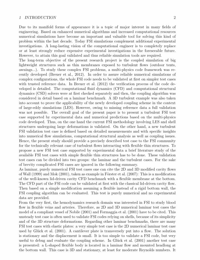
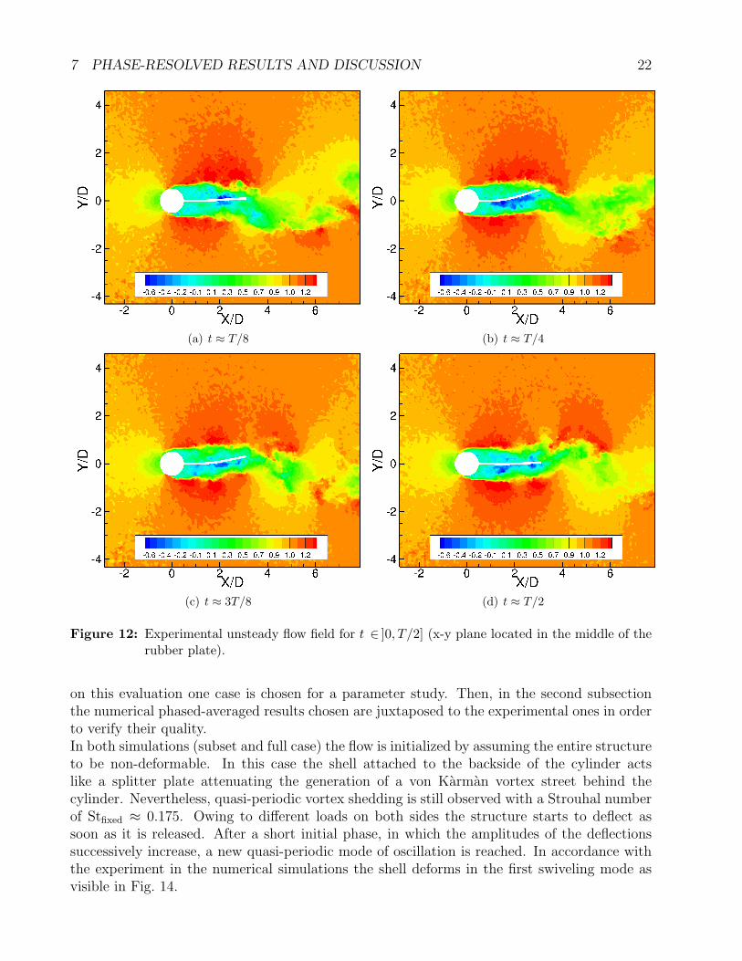
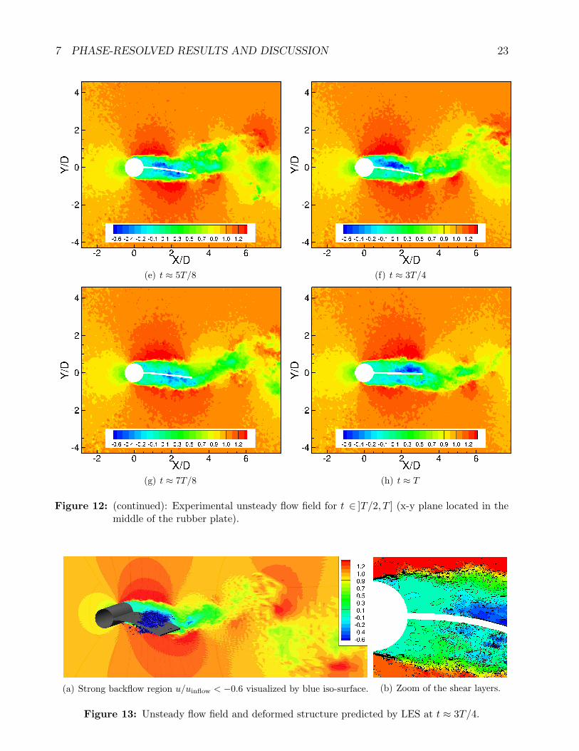
y vary between 0.298and 0.523 and the minima between -0.234 and -0.542. The standard deviations on the extremaare about ±0.05 (±12 % of the mean value of the extrema). Minor variations are observedregarding the period in Figure 11(a). Figure 11(b) and 11(c) show the corresponding experi-mental phase portrait and phase plane, respectively. The phase portrait has a quasi-ellipsoidalform. The monitoring point trajectory plotted in the phase plane describes an inversed “C”,which is typical for the first swiveling mode. The cycle-to-cycle variations in these plots aresmall. Therefore, the FSI phenomenon can be characterized as quasi-periodic.Figure 12 is composed of eight images of the instantaneous flow field (streamwise velocitycomponent) experimentally measured in the x-y plane located in the middle of the rubberplate. These pictures constitute a full period T of the FSI phenomenon arbitrarily chosen.As mentioned before, the shell deforms in the first swiveling mode. Thus, there is only onewave node located at the clamping of the flexible structure. At the beginning of the period(t = 0) the structure is in its undeformed state. Then, it starts to deform upwards and reachesa maximal deflection at t ≈ T/4. Afterwards, the shell deflects downwards until its maximaldeformation at t ≈ 3T/4. Finally the plate deforms back to its original undeformed state andthe end of the period is reached. It should be pointed out that very similar figures as depictedin Fig. 12 could also be shown from the numerical predictions based on LES. Exemplary andfor the sake of brevity, Fig. 13 displays the streamwise velocity component of the flow field ina x-y-plane only at t ≈ 3T/4.As visible in Fig. 12 and in Fig. 13 the flow is highly turbulent, particularly near the cylinder,the flexible structure and in the wake. As expected the LES prediction is capable to resolve

7 PHASE-RESOLVED RESULTS AND DISCUSSION 21
t u / D
Uy/
D
800 820 840 860 880 900-0.6
-0.4
-0.2
0
0.2
0.4
0.6
OO
(a) y-displacement vs. time
Uy/D
Vy/
u
-0.4 0 0.4-0.6
-0.4
-0.2
0
0.2
0.4
0.6
OO
(b) Phase portrait: y-velocity vs. y-displacement
Ux/D
Uy/
D
-0.2 -0.1 0 0.1-0.6
-0.4
-0.2
0
0.2
0.4
0.6
(c) Phase plane: y-displacement vs. x-displacement
Figure 11: Experimental raw signals of dimensionless displacements from a point in the midplaneof the test section located at a distance of 9 mm from the shell extremity.
small-scale flow structures in the wake region and in the shear layers. The strong shear layersoriginating from the separated boundary layers are clearly visible. This is the region wherefor the sub-critical flow the transition to turbulence takes place as visible in the figures. Con-sequently, the flow in the wake region behind the cylinder is obviously turbulent and showscycle-to-cycle variations. That means the flow field in the next periods succeeding the intervaldepicted in Fig. 12 will definitely look slightly different due to the irregular chaotic characterof turbulence. Therefore, in order to be able to compare these results an averaging methodis needed leading to a statistically averaged representation of the flow field. Since the FSIphenomenon is quasi-periodic the phase-averaging procedure presented above is ideal for thispurpose and the results obtained are presented in the next section.
7. Phase-resolved Results and Discussion
The following part is divided into two different sections: in the first one numerical phased-resolved results obtained for the two configurations (full and subset case) are compared. Based
7 PHASE-RESOLVED RESULTS AND DISCUSSION 22
(a) t ≈ T/8 (b) t ≈ T/4
(c) t ≈ 3T/8 (d) t ≈ T/2
Figure 12: Experimental unsteady flow field for t ∈ ]0, T/2] (x-y plane located in the middle of therubber plate).
on this evaluation one case is chosen for a parameter study. Then, in the second subsectionthe numerical phased-averaged results chosen are juxtaposed to the experimental ones in orderto verify their quality.In both simulations (subset and full case) the flow is initialized by assuming the entire structureto be non-deformable. In this case the shell attached to the backside of the cylinder actslike a splitter plate attenuating the generation of a von Karman vortex street behind thecylinder. Nevertheless, quasi-periodic vortex shedding is still observed with a Strouhal numberof Stfixed ≈ 0.175. Owing to different loads on both sides the structure starts to deflect assoon as it is released. After a short initial phase, in which the amplitudes of the deflectionssuccessively increase, a new quasi-periodic mode of oscillation is reached. In accordance withthe experiment in the numerical simulations the shell deforms in the first swiveling mode asvisible in Fig. 14.
7 PHASE-RESOLVED RESULTS AND DISCUSSION 23
(e) t ≈ 5T/8 (f) t ≈ 3T/4
(g) t ≈ 7T/8 (h) t ≈ T
Figure 12: (continued): Experimental unsteady flow field for t ∈ ]T/2, T ] (x-y plane located in themiddle of the rubber plate).
(a) Strong backflow region u/uinflow < −0.6 visualized by blue iso-surface. (b) Zoom of the shear layers.
Figure 13: Unsteady flow field and deformed structure predicted by LES at t ≈ 3T/4.
7 PHASE-RESOLVED RESULTS AND DISCUSSION 24
7.1. Comparison of numerical results
Two numerical setups are used to run the FSI-PfS-1a simulation: the full case and the subsetcase. These configurations differ regarding the geometry and the boundary conditions asdescribed in Section 4.4. The subset case represents a simpler model than the full case requiringless CPU-time (one second real-time is predicted in about 170 hours wall-clock with the subsetcase on 84 processors and in about 310 hours wall-clock with the full case on 142 processors).Similar savings can be achieved with respect to the memory requirements of both cases. Thefull case requires a maximum of 231 Mbytes per core and about 32 Gbytes for all processors.The subset case needs 242 Mbytes per core, which leads to about 20 Gbytes for the entiresimulation. Thus the subset is worth to be considered. The question, however, is whichinfluence these modeling assumptions have on the numerical results?
7.1.1. Full case vs. subset case
Both setups are performed with slightly different material characteristics than defined in Sec-tion 2.4: The Young’s modulus is set to E = 14 MPa, the thickness of the rubber plate is equalto h = 0.002 m, the solid density is ρrubber plate = 1425 kg m−3 and no structural damping isused. The reason is that this comparison was a preliminary study carried out prior to the finaldefinition of the test case. Because of the similitude of the values used here and those definedin Section 2.4 and because of the large CPU-time requested, the comparison of the numericalresults is not repeated with the parameters defined in Section 2.4.
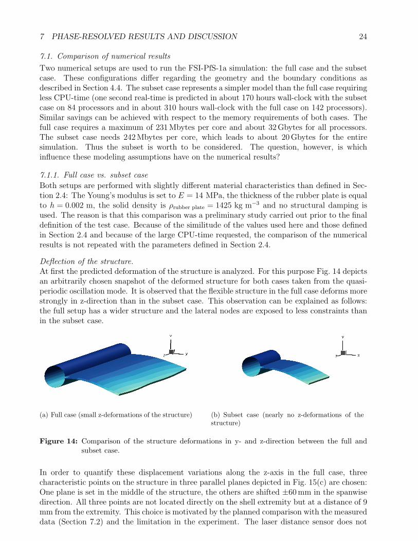
Deflection of the structure.At first the predicted deformation of the structure is analyzed. For this purpose Fig. 14 depictsan arbitrarily chosen snapshot of the deformed structure for both cases taken from the quasi-periodic oscillation mode. It is observed that the flexible structure in the full case deforms morestrongly in z-direction than in the subset case. This observation can be explained as follows:the full setup has a wider structure and the lateral nodes are exposed to less constraints thanin the subset case.
(a) Full case (small z-deformations of the structure) (b) Subset case (nearly no z-deformations of thestructure)
Figure 14: Comparison of the structure deformations in y- and z-direction between the full andsubset case.
In order to quantify these displacement variations along the z-axis in the full case, threecharacteristic points on the structure in three parallel planes depicted in Fig. 15(c) are chosen:One plane is set in the middle of the structure, the others are shifted ±60 mm in the spanwisedirection. All three points are not located directly on the shell extremity but at a distance of 9mm from the extremity. This choice is motivated by the planned comparison with the measureddata (Section 7.2) and the limitation in the experiment. The laser distance sensor does not

7 PHASE-RESOLVED RESULTS AND DISCUSSION 25
allow to follow the structure extremity and thus points at a certain distance from the tail arechosen. The dimensionless y-displacements U∗
y = Uy/D at these three points are monitoredas shown in Fig. 15(a). The following observation can be made: 1. The displacements arein phase. 2. Local differences between the curves are observed in the extrema. 3. Thesevariations are, however, not constant in time. In other words the displacement in one planeis not always bigger than another. The variations reflect some kind of waves in the structurethat move in the spanwise direction. Comparing those three raw signals with the z-averageddisplacements depicted in Fig. 15(b), a maximal difference of 5% regarding the extrema isnoticed. Hence the variations are small. The corresponding z-variations of the subset case areeven smaller (< 0.5%). Therefore, it was decided to continue the analysis by averaging bothcases in z-direction. Notice that by the averaging procedure in z-direction the 3D-problem isreduced to a 2D-problem.The next step is to compare the structure deformations obtained with the full and the sub-set case. Figure 15(b) shows the z-averaged dimensionless y-displacements of both casestaken at 9 mm from the extremity. The frequencies are identically predicted in both cases(fFSInum = 6.96 Hz and StFSInum = 0.11). Minor differences appear in the extrema of theraw signals presented in Fig. 15(b). As before these variations are not constant in timeand thus the maximal values are found irregularly for either the full or the subset case.As a consequence the comparison of the phase-averaged displacement signal (see Fig. 15(d))shows no significant changes between both cases and the coefficient of determination R2 =
1 −∑
i
(
U∗
yi− U∗
yi
)2
/∑
i
(
U∗
yi− U∗
y
)2of the calculated mean phase is close to unity (0.9869
for the full case and 0.9782 for the subset case). U∗
yidenotes the estimated mean value of U∗
y
for the point i. U∗
y is the mean value of all the displacements. The standard deviation for eachpoint of the averaged phase is also computed: the maximum for the full case is 0.055 (dimen-sionless) and for the subset case 0.065 (dimensionless). These values are small compared tothe signal, which is another indication for the reliability of the averaged phase. The subsetcase predicts structure deformations very similar to the full case. In order to check if the FSIresults are quasi identical for the full and the subset case, the phase-resolved flow field has tobe additionally taken into account.
Phase-resolved flow field.The phase-averaging process described in Section 5 delivers the phase-resolved flow fields forthe full and the subset case. In order to compare both just two representative phase-averagedpositions of the FSI problem are chosen to limit this subsection. Figure 16 shows the flowfield in the vicinity of the shell during its maximal deformation at t ≈ T/4 and Fig. 17depicts it close to its undeformed position at t ≈ T , where T denotes the period time of thephase-averaged signal. The figures display the contours of the phase-averaged streamwise andtransverse velocity components. Furthermore, the local error of the velocity magnitude definedby the deviation between the absolute values of the velocity vector of both cases normalizedby the inflow velocity uinflow is depicted. For both positions the results obtained for the subsetand full case are nearly identical. Figures 16(e) and 17(e) underline that the local error ofthe velocity magnitude between both cases is about zero everywhere except in the region nearthe structure. For the position t ≈ T/4 (Fig. 16(e)) small local errors are located behind thestructure in the vortex shedding region. For the position t ≈ T (Fig. 17(e)) the phase-averagedposition of the shell for the subset case differs slightly from the one of the full case. Since theflow field is rapidly changing during the vortex shedding process, this minor deviation in thephase-angle explains the small local errors observed near the structure and in the shear layer.The comparison of the phase-averaged flow fields shows no significant changes between both

7 PHASE-RESOLVED RESULTS AND DISCUSSION 26
t u / D
Uy/
D
50 100 150 200-0.6
-0.4
-0.2
0
0.2
0.4
0.6
oo
(a) Comparison of the numerical raw dimension-less displacements at the three points sketched inFig. 15(c) (full case).
t u / D
Uy/
D
50 100 150 200-0.6
-0.4
-0.2
0
0.2
0.4
0.6
oo
(b) Comparison of the numerical z-averaged dimen-sionless displacements between the full (red) and thesubset (blue) case.
60mm
60mm
9mm.
(c) Position of the monitoring points (in red) for thefull case.
Phase
Uy/
D
0 2 4 6-0.6
-0.4
-0.2
0
0.2
0.4
0.6Full caseSubset case
(d) Comparison of the averaged phase of the fulland the subset case.
Figure 15: Comparison of numerical results for the full case and the subset case.
cases. The subset case predicts the phase-averaged flow field very similar to the full case. Assaid before, the subset setup is simpler and less expensive in CPU-time. Therefore, the subsetcase is very interesting in order to simulate the present test case using LES.
7.1.2. Sensitivity study for the subset case – Dimensional analysis
In order to better understand the test case a dimensional analysis was carried out. The phys-ical quantities of the present FSI problem are: The dynamic viscosity µf , the fluid density ρf ,the inlet velocity uinflow for the fluid; the cylinder diameter D, the dimensions of the rubberplate l, w and h; the Young’s modulus E, the Poisson’s ratio ν and the density of the rubberplate ρrubber plate; To describe the FSI phenomenon the FSI frequency fFSI, the displacementextrema Uy|max
and Uy|minare chosen. These 13 physical quantities lead to 10 dimensionless
parameters: The Reynolds number Re = ρfuinflowD/µf for the fluid; the length ratios w/l, h/l,D/l for the geometry; ν for the material of the rubber plate; The density ratio ρf/ρrubber plate,

7 PHASE-RESOLVED RESULTS AND DISCUSSION 27
the Cauchy number Cy = ρfu2inflow/E (as defined in De Langre (2002)), the extrema of the
dimensionless y-displacements U∗
y
∣
∣
max= Uy|max
/D and U∗
y
∣
∣
min= Uy|min
/D and the Strouhalnumber StFSI = fFSID/uinflow for the FSI coupling.
In the present experimental investigation the operating conditions for the fluid are well-known.The length and the width of the rubber plate are well defined, too. Therefore, the Reynoldsnumber Re, the geometrical ratios w/l and D/l are fixed in the sensitivity study.
• On the contrary, as mentioned in Section 2.1, the material is natural rubber and tomanufacture a perfectly homogeneous 2 mm plate is not easy. The experimental mea-surements show that the thickness varies between 0.002 and 0.0022 m. Two values of hare tested: the theoretical value of 0.002 m and the average value 0.0021 m. Consequently,the geometrical ratio h/l will be taken into account in the sensitivity study.
• The density of the rubber plate ρrubber plate is determined by a scale and the volume ofthe structure. Due to the dependency of this volume on the plate thickness the densitydetermination can be inaccurate. As an additional dimensionless parameter the densityratio ρf/ρrubber plate is a part of the sensitivity study.
• The last parameter of the structure is the Young’s modulus, because it has an importantinfluence on the modeling of the material. A range of values for E and consequently ofCy is tested to evaluate this influence.
The dimensional analysis presented here will also be reduced to the six following dimensionlessnumbers: the density ratio ρf/ρrubber plate, the geometrical ratio h/l, the Cauchy number Cy,the dimensionless y-displacement extrema U∗
y
∣
∣
maxand U∗
y
∣
∣
minand the Strouhal number StFSI.
All the tests were carried out without structural damping and are summarized in Table 4. Thefull case used in Section 7.1.1 and the experimental results are also added as references. Eachsimulation was done for a time interval of 4 s physical time and comprises about 27 swivelingperiods. Relative errors between the numerical and experimental values are given.
The following results and trends can be seen:
• By varying the Young’s modulus E between 8 and 16 MPa (240×10−6 ≥ Cy ≥ 120×10−6)it is possible to control the mode of the FSI phenomenon. Thus E (or the Cauchy number)turns out to be the most crucial material parameter. With E smaller than 9 MPa (Cy≥ 213×10−6), the system oscillates in the second swiveling mode (similar to the secondbending mode presented in Fig. B.25). With E larger than 12 MPa (Cy ≤ 160×10−6)the structure deflection is dominated by the first bending mode of the structure. For aYoung’s modulus between 9 and 12 MPa (213×10−6 ≥ Cy ≥ 160×10−6) a mode transitionphase appears in which both swiveling modes are apparent. In this situation the y-displacements of the flexible structure extremity are no longer quasi-periodic and cannot be described by a unique frequency.
• Non-negligible variations in the density (1320 kg m−3 ≤ ρrubber plate ≤ 1725 kg m−3)(0.757 ≥ ρf/ρrubber plate ≥ 0.580) for a fixed thickness (h = 0.002 m) and Young’s modulus(E = 14 MPa) do not drastically change the results of the frequency and of the meanperiod extrema. The FSI frequency fFSI (respectively the Strouhal number StFSI) slightlydecreases with the increase of the density.

7PHASE-R
ESOLVED
RESULTSAND
DISCUSSIO
N28
Case Materials parameters Dimensionless numbers Results
Thickness Density E h/l ρf Cy fFSI StFSI Error U∗
y
∣
∣
maxError U∗
y
∣
∣
minError Comments
h (mm) (kg m−3) (MPa) ρrubber plate (Hz) (%) (%) (%)
Subset case
2 1320 14 0.033 0.757 137×10−6 7.00 0.1112 -1.40 0.460 10.1 -0.488 -16.4 first swiveling mode
2 1425 14 0.033 0.702 137×10−6 6.96 0.1106 -2.02 0.463 10.6 -0.457 -8.9 first swiveling mode
2 1725 14 0.033 0.580 137×10−6 6.94 0.1102 -2.22 0.458 9.6 -0.478 -13.9 first swiveling mode
2 1425 8 0.033 0.702 240×10−6 - - - - - - - second swiveling mode
2 1425 9 0.033 0.702 213×10−6 - - - - - - - second mode+transition
2 1425 10 0.033 0.702 192×10−6 - - - - - - - second mode+transition
2 1425 11 0.033 0.702 174×10−6 - - - - - - - transition
2 1425 12 0.033 0.702 160×10−6 - - - - - - - transition+first mode
2 1425 14 0.033 0.702 137×10−6 6.96 0.1106 -2.02 0.463 10.6 -0.457 -8.9 first swiveling mode
2 1425 15 0.033 0.702 129×10−6 7.04 0.1118 -0.84 0.448 7.2 -0.481 -14.6 first swiveling mode
2 1425 16 0.033 0.702 120×10−6 7.10 0.1128 -0.01 0.471 12.6 -0.473 -12.7 first swiveling mode
2.1 1360 14 0.035 0.735 137×10−6 7.00 0.1112 -1.38 0.463 10.6 -0.471 -12.2 first swiveling mode
2.1 1360 15 0.035 0.735 129×10−6 7.07 0.1123 -0.50 0.461 10.3 -0.479 -14.0 first swiveling mode
2.1 1360 16 0.035 0.735 120×10−6 7.08 0.1125 -0.25 0.456 9.1 -0.464 -10.6 first swiveling mode
2.1 1360 18 0.035 0.735 107×10−6 7.13 0.1133 0.36 0.447 6.8 -0.462 -10.2 first swiveling mode
2.1 1360 20 0.035 0.735 96×10−6 7.20 0.1144 1.32 0.452 8.0 -0.461 -9.7 first swiveling mode
Full case 2 1425 14 0.033 0.702 137×10−6 6.96 0.1106 -2.02 0.465 11.2 -0.473 -12.6 first swiveling mode
Experiments 7.10 0.1128 - 0.418 - -0.420 - first swiveling mode
Table 4: Parameter study for the subset case of the FSI test case (without structural damping).

7 PHASE-RESOLVED RESULTS AND DISCUSSION 29
• Comparing the results for both thicknesses for the range 14 MPa ≤ E ≤ 16 MPa, it isobvious that a mild variation of the thickness of the rubber plate (0.1 mm, equivalent to5 %) has a non-negligible influence on the extrema of the mean period and no significantinfluence on the frequency.
• Overall the frequency of the FSI phenomenon fFSI (respectively the Strouhal numberStFSI) is very well predicted (relative error under 2.22 %) for all tested parameters leadingto the first swiveling mode.
• Comparing the results for the density ρrubber plate = 1360 kg m−3 in the range 14 MPa ≤E ≤ 20 MPa, we observe that the FSI frequency fFSI (respectively the Strouhal numberStFSI) slightly increases with the Young’s modulus and that the displacement extremadecrease.
In summary, the parameter study shows that the Young’s modulus (or the dimensionlessnumber of Cauchy Cy) is the most important parameter: It controls the swiveling modeof the flexible structure. Furthermore, it can be observed that mild modifications of theshell thickness (or of the geometrical ratio h/l) have a certain effect on the predicted FSIphenomenon. Contrarily, this parameter study shows that variations of the density ratio donot have major influence on the predictions. Therefore, errors in the density measurementdo not play an important role. With the support of these extensive preliminary numericalinvestigations we can now compare the final numerical results with the experiment.
7.2. Comparison between numerical and experimental results
The investigations presented in Section 7.1.1 based on slightly different material characteristicsthan defined in Section 2.4 have shown that the subset case permits a gain in CPU-time butnevertheless nearly identical results as the full case. Therefore, the numerical computationwith the structural parameters defined in Section 2.4 (E = 16 MPa, h = 0.0021 m, ρrubber plate
= 1360 kg m−3) is carried out for the subset case.Two simulations are considered: One with the structural damping defined in Appendix B, theother one without damping. These results are compared with the experimental data to checktheir accuracy. In order to quantitatively compare the experimental and numerical data, bothare phase-averaged as explained in Section 5. Similar to the numerical comparison presentedin Section 7.1.1 the displacement of the structure will be first analyzed and then the phase-resolved flow field is considered.
7.2.1. Deflection of the structure
The structure contour of the phased-averaged experimental results for the reference period isdepicted in Fig. 18. Obviously, the diagram represents the first swiveling mode of the FSI phe-nomenon showing only one wave mode at the clamping. Figure 19(a) depicts the experimentaldimensionless raw signal obtained at a point located in the midplane at a distance of 9 mmfrom the shell extremity. Figure 19(b) shows the numerical signal predicted without struc-tural damping and Fig. 19(c) the one computed with damping. Applying the phase-averagingprocess the mean phase of the FSI phenomenon for the experiment and for the simulationsis generated. The outcome is presented in Fig. 19(d) with the phase as the abscissa and thedimensionless displacement U∗
y = Uy/D as the ordinate. The amplitudes of the experimentalsignal varies more than in the predictions. Therefore, the maximal standard deviation of eachpoint of the averaged phase is for the experiment bigger (0.083) than for the simulation (0.072with and without damping). In order to check the reliability of the computed mean phase
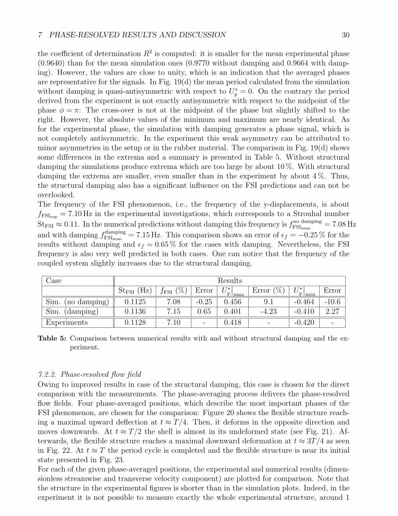
7 PHASE-RESOLVED RESULTS AND DISCUSSION 30
the coefficient of determination R2 is computed: it is smaller for the mean experimental phase(0.9640) than for the mean simulation ones (0.9770 without damping and 0.9664 with damp-ing). However, the values are close to unity, which is an indication that the averaged phasesare representative for the signals. In Fig. 19(d) the mean period calculated from the simulationwithout damping is quasi-antisymmetric with respect to U∗
y = 0. On the contrary the periodderived from the experiment is not exactly antisymmetric with respect to the midpoint of thephase φ = π: The cross-over is not at the midpoint of the phase but slightly shifted to theright. However, the absolute values of the minimum and maximum are nearly identical. Asfor the experimental phase, the simulation with damping generates a phase signal, which isnot completely antisymmetric. In the experiment this weak asymmetry can be attributed tominor asymmetries in the setup or in the rubber material. The comparison in Fig. 19(d) showssome differences in the extrema and a summary is presented in Table 5. Without structuraldamping the simulations produce extrema which are too large by about 10 %. With structuraldamping the extrema are smaller, even smaller than in the experiment by about 4 %. Thus,the structural damping also has a significant influence on the FSI predictions and can not beoverlooked.The frequency of the FSI phenomenon, i.e., the frequency of the y-displacements, is aboutfFSIexp = 7.10 Hz in the experimental investigations, which corresponds to a Strouhal number
StFSI ≈ 0.11. In the numerical predictions without damping this frequency is fno dampingFSInum
= 7.08 Hz
and with damping fdampingFSInum
= 7.15 Hz. This comparison shows an error of ǫf = −0.25 % for theresults without damping and ǫf = 0.65 % for the cases with damping. Nevertheless, the FSIfrequency is also very well predicted in both cases. One can notice that the frequency of thecoupled system slightly increases due to the structural damping.
Case ResultsStFSI (Hz) fFSI (%) Error U∗
y
∣
∣
maxError (%) U∗
y
∣
∣
minError
Sim. (no damping) 0.1125 7.08 -0.25 0.456 9.1 -0.464 -10.6Sim. (damping) 0.1136 7.15 0.65 0.401 -4.23 -0.410 2.27
Experiments 0.1128 7.10 - 0.418 - -0.420 -
Table 5: Comparison between numerical results with and without structural damping and the ex-periment.
7.2.2. Phase-resolved flow field
Owing to improved results in case of the structural damping, this case is chosen for the directcomparison with the measurements. The phase-averaging process delivers the phase-resolvedflow fields. Four phase-averaged positions, which describe the most important phases of theFSI phenomenon, are chosen for the comparison: Figure 20 shows the flexible structure reach-ing a maximal upward deflection at t ≈ T/4. Then, it deforms in the opposite direction andmoves downwards. At t ≈ T/2 the shell is almost in its undeformed state (see Fig. 21). Af-terwards, the flexible structure reaches a maximal downward deformation at t ≈ 3T/4 as seenin Fig. 22. At t ≈ T the period cycle is completed and the flexible structure is near its initialstate presented in Fig. 23.For each of the given phase-averaged positions, the experimental and numerical results (dimen-sionless streamwise and transverse velocity component) are plotted for comparison. Note thatthe structure in the experimental figures is shorter than in the simulation plots. Indeed, in theexperiment it is not possible to measure exactly the whole experimental structure, around 1

8 AVAILABLE DATA FOR COMPARISON 31
mm at the end of the structure is missing. As in Section 7.1 an additional figure shows theerror between the simulation and the experiment for the velocity magnitude.At t ≈ T/4 (see Fig. 20), when the structure is in its maximal upward deflection, the accel-eration zone above the structure has reached its maximum. The acceleration area below therubber plate is growing. Both phenomena are correctly predicted in the simulations. Thecomputed acceleration area above the structure is slightly overestimated. However, the localerror is mostly under 20 %.The separation points at the cylinder are found to be in close agreement between measurementsand predictions. Accordingly, also the location of the shear layers shows a good agreement be-tween simulations and experiments. The shedding phenomenon behind the structure generatesa turbulent wake, which is correctly reproduced by the computations. Owing to the phase-averaging procedure, as expected all small-scale structures are averaged out.At t ≈ T/2 (see Fig. 21), the shell is near its undeformed state. The acceleration zone abovethe structure has shrunk in favor of the area below the rubber plate. Regarding these areasthe predictions show a very good agreement with the measurements (marginal local errors).The predicted wake directly behind the structure matches the measured one.At t ≈ 3T/4 (see Fig. 22), the downward deformation of the shell is maximal, the flow is thesymmetrical to the flow observed at t ≈ T/4 with respect to y/D = 0. Again the accelerationareas around the structure show a very good agreement with the measurements. Once morethe wake is correctly predicted in the near-field of the structure.At t ≈ T (see Fig. 23) the flow is symmetrical to the flow observed at t ≈ T/2 with respect toy/D = 0. The computed acceleration area above the structure is slightly overestimated, butthe local error is under 20 %. The wake is again correctly predicted except directly after theflexible structure.For every position the local error is mostly under 20 %. In the error plot the areas with a biggerlocal error are near the structure and in the shear layers. This can be explained by the fact thatnear the structure and in the shear layers the gradients of the flow quantities are large. Sincethe mesh used for the simulation is much finer than the PIV measurement grid, the accuracyof the numerical solution is much higher than the precision of the PIV measurements in theseregions. It is also difficult to measure the flow accurately in the direct vicinity of a body dueto reflections of the laser light at the surface. Another reason is that the error expected bythe PIV method is more important for low flow velocities. Close to the flexible structure anddirectly after its tail the flow velocity is small, which at least partially explains the deviationsobserved between the experimental and numerical results.In summary, for every position the computed flow is in good agreement with the measuredone. The shedding phenomenon behind the cylinder and the positions of the vortices convecteddownstream are correctly predicted.
8. Available Data for Comparison
The described benchmark FSI-PfS-1a is supposed to test, evaluate and improve numerical FSIcodes. Therefore, the authors support all interested groups by the experimental and numericaldata presented in this paper. For this purpose the data are made available on the ERCOFTACKnowledge Base Wiki in the category ’Flow around Bodies’ accessible as case 2–13 under
http://qnet-ercoftac.cfms.org.uk/w/index.php/UFR_2-13.
Available for comparison are:
• the data for the structural test cases described in Appendix A.

8 AVAILABLE DATA FOR COMPARISON 32
• the 23 single phase-averaged two-dimensional reference velocity fields of the PIV mea-surement series and the corresponding numerical data used in Section 7.2;
• the raw and phase-averaged data of the displacement of the flexible structure.
• animations of the test case.

8 AVAILABLE DATA FOR COMPARISON 33
(a) Full case (streamwise velocity component) (b) Full case (transverse velocity component)
(c) Subset case (streamwise velocity component) (d) Subset case (transverse velocity component)
(e) Absolute local error (velocity magnitude) in %
Figure 16: Comparison of the results for the full and subset case; phase-averaged data at t ≈ T/4.

8 AVAILABLE DATA FOR COMPARISON 34
(a) Full case (streamwise velocity component) (b) Full case (transverse velocity component)
(c) Subset case (streamwise velocity component) (d) Subset case (transverse velocity component)
(e) Absolute local error (velocity magnitude) in %
Figure 17: Comparison of the results for the full and subset case; phase-averaged data at t ≈ T .

8 AVAILABLE DATA FOR COMPARISON 35
x/D
01
23
y/D
-1
0
1
period
T
T/2
T/4
3T/4
Figure 18: Experimental structural results: Structure contour for the reference period.

8 AVAILABLE DATA FOR COMPARISON 36
t u / D
Uy/
D
50 100 150 200-0.6
-0.4
-0.2
0
0.2
0.4
0.6
OO
(a) Experimental raw signal: Dimensionless dis-placement.
t u / D
Uy/
D
50 100 150 200-0.6
-0.4
-0.2
0
0.2
0.4
0.6
OO
(b) Numerical raw signal (without damping): Di-mensionless displacement.
t u / D
Uy/
D
50 100 150 200-0.6
-0.4
-0.2
0
0.2
0.4
0.6
OO
(c) Numerical raw signal (with damping): Dimen-sionless displacement.
Phase
Uy/
D
0 2 4 6-0.6
-0.4
-0.2
0
0.2
0.4
0.6experimentspredictions dampingprediction no damping
(d) Comparison of the averaged phase of the exper-imental and numerical data.
Figure 19: Comparison of experimental and numerical results; raw signals and averaged phases ofa point located in the midplane at 9mm distance from the shell extremity.

8 AVAILABLE DATA FOR COMPARISON 37
(a) PIV data (streamwise velocity component) (b) PIV data (transverse velocity component)
(c) FSI simulation (streamwise velocity component) (d) FSI simulation (transverse velocity component)
(e) Absolute local error (velocity magnitude) in %
Figure 20: Comparison of experimental and numerical results (subset case with damping, see Ta-ble 5); phase-averaged data at t ≈ T/4.

8 AVAILABLE DATA FOR COMPARISON 38
(a) PIV data (streamwise velocity component) (b) PIV data (transverse velocity component)
(c) FSI simulation (streamwise velocity component) (d) FSI simulation (transverse velocity component)
(e) Absolute local error (velocity magnitude) in %
Figure 21: Comparison of experimental and numerical results (subset case with damping, see Ta-ble 5); phase-averaged data at t ≈ T/2.

8 AVAILABLE DATA FOR COMPARISON 39
(a) PIV data (streamwise velocity component) (b) PIV data (transverse velocity component)
(c) FSI simulation (streamwise velocity component) (d) FSI simulation (transverse velocity component)
(e) Absolute local error (velocity magnitude) in %
Figure 22: Comparison of experimental and numerical results (subset case with damping, see Ta-ble 5); phase-averaged data at t ≈ 3T/4.

8 AVAILABLE DATA FOR COMPARISON 40
(a) PIV data (streamwise velocity component) (b) PIV data (transverse velocity component)
(c) FSI simulation (streamwise velocity component) (d) FSI simulation (transverse velocity component)
(e) Absolute local error (velocity magnitude) in %
Figure 23: Comparison of experimental and numerical results (subset case with damping, see Ta-ble 5); phase-averaged data at t ≈ T .

9 CONCLUSIONS 41
9. Conclusions
A new FSI validation test case denoted FSI-PfS-1a is proposed. The definition of the test caseis driven by the idea to setup a well-defined but nevertheless challenging validation test casefor fluid-structure interaction in the turbulent flow regime. A rigid front cylinder and a flexiblemembranous rubber tail attached to the backside of the cylinder form the structure which isexposed to a uniform inflow at a low turbulence level. Thus three critical issues of precursorbenchmarks are circumvented, i.e., an additional degree of freedom of a rotating front cylinder,an extremely thin flexible structure and an additional weight at the end of the membranousstructure. The investigations comprise three parts.First, two dynamic structural tests were carried out experimentally and numerically in orderto evaluate an appropriate material model and to check and evaluate the material parametersof the rubber (Young’s modulus, structural damping). This preliminary work has shown thatthe St. Venant-Kirchhoff material model is sufficient to describe the deflection of the flexiblestructure.Second, detailed experimental investigations in a water tunnel using optical measurement tech-niques for both, the fluid flow and the structure deformation, were carried out. A quasi-periodicoscillating flexible structure in the first swiveling mode with a corresponding Strouhal numberof about StFSI = 0.11 is found. A post-processing of the extensive data sets delivered thephase-averaged flow field and the structural deformations.Third, various simulations relying on a newly developed FSI simulation tool combining apartitioned solution strategy with an eddy-resolving scheme (LES) were performed. A subsetcase and full case are taken into account. Owing to the wider structure and less constraintsof the lateral nodes the deformations in the spanwise direction were found to be larger in thefull case reflecting some kind of mild waves in the structure. Nevertheless, in relation to thedeformation of the structure in cross-flow direction the spanwise deflections are insignificant,especially for the comparison of the phase-averaged signals.A study on three parameters for the subset case without structural damping yields that theYoung’s modulus (or the Cauchy number) has a very important influence on the system. Itcontrols in which swiveling mode the flexible structure oscillates. The thickness of the rubberplate h/D plays a role in the results, too, but not so significant as the Young’s modulus. Theparameter with the least effect on the FSI simulations is the density ratio of the body: limitedvariations of the density do not have major influence on the predictions.As usual for rubber material, a certain level of structural damping has to be expected. Tomodel this phenomenon in a simple and straightforward way, classical Rayleigh damping isused and adjusted based on one of the pure structural tests presented in the appendix. TheFSI simulations with and without structural damping are compared with the experiment. Itturns out that the structural damping can not be ignored in the present case and significantlyaffects the deflection of the structure. Without taking the damping into account the structuraldeflections are overpredicted. Including the simple damping model improves the results. Theeddy-resolving FSI simulations are found to be in close agreement with the experiment for everyposition of the flexible structure. Merely the amplitudes of the deflections are slightly underpre-dicted with damping. Nevertheless, the shedding phenomenon behind the cylinder/structureand the positions of the vortices convected downstream are correctly predicted. Furthermore,the FSI frequency found in the simulations matches particularly well the measured one.The described test case FSI-PfS-1a is a part of a series of reference test cases designed toimprove numerical FSI codes. A second test case FSI-PfS-2a is described in Kalmbach andBreuer (2013). The geometry is similar to the first one: A fixed rigid cylinder with a plateclamped behind it. However, this time a rear mass is added at the extremity of the flexible

APPENDIX A DESCRIPTION OF PURE STRUCTURAL TESTS 42
structure and the material (para-rubber) is less stiff. The flexible structure deforms in thesecond swiveling mode and the structure deflections are completely two-dimensional and larger.For each test case all the experimental data are available on demand.
Acknowledgments
The project is financially supported by the Deutsche Forschungsgemeinschaft under the con-tract numbers BR 1847/12-1 and BL 306/26-1. The computations were partially carried outon the German Federal Top-Level Computer SuperMUC/SuperMIG at LRZ Munich under thecontract number pr47me. We would like to thank the Draftex Automotive GmbH in Grefrathfor providing the rubber material and the corresponding measurements of its characteristicproperties. Special thanks goes also to H. Lienhart (LSTM Erlangen) for the construction ofthe water channel and many helpful advices regarding the experimental setup. All kinds ofsupport are gratefully acknowledged.
Appendix A. Description of pure structural tests
The measurements of the different structural test cases and the respective numerical simulationswith different parameter sets serve two different purposes. On the one hand, the characteristicmodel parameters should be determined and checked by parametric studies. On the other hand,it should be verified that with the chosen material models, the correct structural behavior canbe recovered in the predictions.Both pure structural cases consist of a flexible rubber plate (0.06 m × 0.177 m × 0.0021 m)clamped between a rigid cylinder (ρcylinder = 3146 kg/m3) and two half cylinders made of brass(ρbar = 8450 kg/m3) at the other end. These constrain the respective two edges of the plate todeform without warping, which results in a clear and easy to measure deformation state. Thetest cases use a setup with a vertical alignment of the plate (see Fig. A.24).
Free oscillation test.In the first test case, the cylinder (C1) is fixed. To initiate an oscillation, the free end isdeflected by a well-defined horizontal movement Uy and then released, such that a decayingvibration can be accurately traced using the laser distance sensor described in Section 3.2.
Forced periodic oscillation test.For the second test scenario, the support of the cylinder (C1) at the upper margin is a rotatablebearing. This cylinder is stimulated by a periodic excitation of φ(t) = φmax sin(ω t) + φoffset
with a maximal angular deflection of φmax = 6.1◦ and a frequency of ω = 18.33 s−1 resulting inan unsteady deformation of the rubber plate. The offset of φoffset = +0.5◦ is required because ofthe experimental setup of the crank drive that creates a slightly asymmetric angular excitationof the actuated upper cylinder. However, since this shift can be easily deducted from themeasurements, it is not mentioned in the following. The inertia of the end bar increasesthe displacements and also modifies the deflection behavior of the flexible structure to non-linear deformations. The low oscillation frequency is chosen to reduce the velocity-relateddeformation effects of the rubber material. As before the laser distance sensor described inSection 3.2 detects the displacements with a high measuring frequency.

APPENDIX B VALIDATION OF THE STRUCTURAL MODEL 43
22
2
y
x
C1
rubber plate
brass profiles
x measuring position
g
*
* *
635
x
Figure A.24: Sketch of the geometrical configuration of the structural tests.
Appendix B. Validation of the structural model
To demonstrate the applicability of solid as well as shell elements for the structural finite-element model, comparative simulations were carried out for the structural test cases mentionedin Appendix A. In order to separate the effects of structural damping, the cross-comparisonof models was done via the computation of eigenfrequencies and the corresponding structuraleigenmodes which are shown in Fig. B.25. Note that the shell models are visualized with theirthickness to demonstrate the regions of the more bulky parts. It can be seen that the maindynamic deformation mechanisms which are relevant for the FSI benchmark (e.g., the firstand second plate bending modes instead of thickness vibration modes) are perfectly recoveredby the solid as well as by the dimensionally reduced shell model. Special care was takento model the translational and rotational inertia of the cylindrical weight appropriately forthe shell setup. As can be immediately concluded from the fact of a pure two-dimensionaldiscretization compared to a full resolution of the three-dimensional body, the computationsusing shell elements were 8 times faster and thus, remarkably less computationally expensive.For the correct reproduction of the transient structural test cases, the consideration of thepre-stressing effect of the cylinder’s weight is crucial and may not be neglected. This issue wasinvestigated by doing eigenfrequency evaluations with and without considering the weight of thecylinder: In the former case, first a static simulation of the benchmark setup with self-weightwas carried out and the resulting stresses were transferred to the initial structural configurationfor the eigenfrequency analysis. As a consequence, the measured first eigenfrequency of about4.55 Hz was computed as 4.69 Hz, whereas without consideration of the pre-stress induced byself-weight the stiffness of the structure was under-estimated and thus the first eigenfrequencywas determined to be about 4.16 Hz.Due to the usual dynamic behavior of rubber, a certain level of damping has to be expected.To represent this adequately in the numerical simulation, various approaches are possible.However, damping in a vibrating structure is a complex phenomenon with various sources (Pe-tersen, 2000). The goal within this benchmark description is to provide a simple modeling

APPENDIX B VALIDATION OF THE STRUCTURAL MODEL 44
Figure B.25: Comparison of the first three structural eigenmodes for solid (upper row) as well asshell models (lower row) for the pure CSD setup presented in Appendix A.
for the damping effects to enable the computation with standard finite-element codes withoutadapting them. Moreover, based on the experimental observations it can be observed, thatwithin the proposed FSI benchmark only the lowest eigenmodes (nearly exclusively the firstbending mode shown in Fig. B.25) of the structure are excited. A proper choice for the damp-ing model is therefore the Rayleigh damping: all damping effects are summarized in a velocityproportional damping matrix D which is composed of a linear combination of the mass matrixM and the (initial) stiffness matrix K0:
D = αM + βK0 . (B.1)
According to Clough and Penzien (1993), the two open Rayleigh damping factors α and βcan be evaluated by solving a pair of equations, in case that two damping ratios and therespective frequencies are known. Since the FSI test case shows nearly only oscillations in thefirst eigenmode, it was decided to take only one damping factor. More precisely, the stiffnessproportional damping factor β is considered to be evaluated and the mass proportional quantityα is assumed to be zero. The reason for this decision is that the stiffness proportional dampingis considered to be more realistic (see, e.g., Kratzig et al., 1996) in this case, since the massproportional damping factor results in decaying damping effects on higher modes. The dampingparameter β is calibrated with the free oscillation test, introduced in Appendix A and it isassumed that it can be used for the FSI simulations accordingly.
Free oscillation test.In order to compute this test Carat++ uses a grid with 10×10 quadrilateral 7-parameter shellelements mentioned above. The generalized-α method is used with a time step of 4×10⁻³ s.Abaqus uses the meshes presented in Fig. B.25. The Abaqus shell elements are S8R. The HHTtime discretization is set with an initial time step of 1×10⁻³ s. Then, the adaptive time stepcontrol is enabled with TRANSIENT FIDELITY.Based on some rough estimations the value could be found to be in the range between 0.01 and0.02. Further parametric studies and cross-comparisons with the experimental data lead to avalue β = 0.017. Computed results for the free oscillation test and the measured deformationsare displayed in Fig. B.26. It can be seen that with this choice of the damping parameters

APPENDIX C GRID DEPENDENCY STUDY FOR THE STRUCTURAL MODEL 45
the experimentally observed decay behavior of the oscillation due to the initial deflection iscaptured very well.
t [s]
Y/D
0 0.5 1 1.5
-1
-0.5
0
0.5
1 ExperimentSimulation ABAQUSSimulation CARAT++
Figure B.26: Free oscillation test: Comparison of y-deformations of the point marked as measuringposition in Fig. A.24 between structural simulations and experiment.
Forced periodic oscillation test.The forced periodic oscillation test is also computed with Abaqus using shell and solid finiteelements with the settings mentioned above and the material parameters provided. The sim-ulation results of the shell model are exemplary compared to the measured deformations inFig. B.27. A time period of a fully developed oscillation is chosen, to avoid transient effectsduring the startup procedure of the experiment. Structural damping is used in the simulationand adjusted as described above. The very good agreement of numerical and experimentaldata supports the chosen material data summarized in Table 3. Thus the structural modelingas an important part of the overall FSI setup is carefully checked.
Appendix C. Grid dependency study for the structural model
As a preliminary investigation for the choice of a proper structure mesh, a small test casewith a constant pressure distribution on one plate surface is carried out using the materialparameters defined in Section 2.4. The magnitude of the pressure is chosen such that thefinal tip deformation is in the range of the maximally expected tip deflection of the flexiblestructure in the FSI case. This load scenario is computed with a sequence of systematicallyrefined meshes (using quadrilateral four-node shell elements) for the quadratic structure usedin the subset case and for the rectangular one used in the full case. The tip deformationsobtained are summarized in Table C.6. Moreover, a cross-check by a simulation using a veryfine mesh of solid elements shows a deviation in the tip displacement of less than 1 %. As aresult of this grid independency study, a mesh with 30 shell elements in streamwise directioncan be considered as converged for both cases. Astonishingly, even a mesh with only 10 shellelements of the used type in streamwise direction could be seen as reasonable for a deflectioncomparable to the one observed in the FSI experiments. Thus in order to save CPU-time 10× 10 and 10 × 30 shell elements are applied in the FSI prediction of the subset and the fullcase, respectively.

REFERENCES 46
t [s]
Y/D
22 22.5 23 23.5 24-1
-0.5
0
0.5
1
ExperimentSimulation
Figure B.27: Forced periodic oscillation test: Comparison of measured and computed y-displacements of the point marked as measuring position in Fig. A.24 (Note thatthe experimental data are shifted by the offset φoffset as mentioned in the text).
Mesh (Length × Width ) Utip [m] Error
Subset case
10 × 10 1.31466e-02 0.6 %20 × 20 1.32076e-02 0.1 %30 × 30 1.32248e-02 0.01 %40 × 40 1.32267e-02 Ref.
Full case
10 × 30 1.31873e-02 0.4 %20 × 60 1.32281e-02 0.1 %30 × 90 1.32413e-02 0.01 %40 × 120 1.32426e-02 Ref.
Table C.6: Grid study for the structure with the CSD solver Carat++.
References
Adrian, R. J., 1991. Particle-imaging techniques for experimental fluid mechanics. AnnualReview of Fluid Mechanics 23 (1), 261–304.
Balint, T. S., Lucey, A. D., 2005. Instability of a cantilevered flexible plate in viscous channelflow. Journal of Fluids and Structures 20 (7), 893–912.
Bischoff, M., 1999. Theorie und Numerik einer dreidimensionalen Schalenformulierung. Ph.D.thesis, Institut fur Baustatik, Universitat Stuttgart, Germany.
Bischoff, M., Ramm, E., 1997. Shear deformable shell elements for large strains and rotations.Int. Journal for Numerical Methods in Engineering 40 (23), 4427–4449.
Bischoff, M., Ramm, E., 2000. On the physical significance of higher-order kinematic andstatic variables in a three-dimensional shell formulation. Int. Journal of Solids and Structures37 (46), 6933–6960.
REFERENCES 47
Bischoff, M., Wall, W. A., Bletzinger, K.-U., Ramm, E., 2004. Models and finite elements forthin-walled structures. In: Stein, E., De Borst, R., Hughes, T. J. R. (Eds.), Encyclopedia ofComputational Mechanics. Vol. 2. John Wiley & Sons Ltd, Chichester, pp. 59–138.
Bletzinger, K.-U., Wuchner, R., Daoud, F., Camprubı, N., 2005. Computational methodsfor form finding and optimization of shells and membranes. Computer Methods in AppliedMechanics and Engineering 194 (30), 3438–3452.
Bletzinger, K.-U., Wuchner, R., Kupzok, A., 2006. Algorithmic treatment of shells and freeform-membranes in FSI. In: Bungartz, H.-J., Schafer, M. (Eds.), Fluid-Structure Interaction.Vol. 53 of Lecture Notes in Computational Science and Engineering, LNCSE. Springer,Heidelberg, pp. 336–355.
Boyer, F., De Nayer, G., Leroyer, A., Visonneau, M., 2011. Geometrically exact Kirchhoff beamtheory: Application to cable dynamics. Journal of Computational and Nonlinear Dynamics6, 041004.
Breuer, M., 2002. Direkte Numerische Simulation und Large-Eddy Simulation turbulenterStromungen auf Hochleistungsrechnern. Habilitationsschrift, Universitat Erlangen–Nurn-berg, Berichte aus der Stromungstechnik. Shaker Verlag, Aachen, Germany.
Breuer, M., De Nayer, G., Munsch, M., Gallinger, T., Wuchner, R., 2012. Fluid-structureinteraction using a partitioned semi-implicit predictor-corrector coupling scheme for theapplication of large-eddy simulation. Journal of Fluids and Structures 29, 107–130.
Buchter, N., Ramm, E., 1992. Shell theory versus degeneration – A comparison in large rotationfinite element analysis. Int. Journal for Numerical Methods in Engineering 34 (1), 39–59.
Buchter, N., Ramm, E., Roehl, D., 1994. Three-dimensional extension of non-linear shell for-mulation based on the enhanced assumed strain concept. Int. Journal for Numerical Methodsin Engineering 37 (15), 2551–2568.
Bungartz, H.-J., Mehl, M., Schafer, M. (Eds.), 2010. Fluid Structure Interaction II: Mod-elling, Simulation, Optimization. Vol. 73 of Lecture Notes in Computational Science andEngineering, LNCSE. Springer, Heidelberg.
Cantwell, B., Coles, D., 1983. An experimental study of entrainment and transport in theturbulent near wake of a circular cylinder. Journal of Fluid Mechanics 136 (1), 321–374.
Chung, J., Hulbert, G. M., 1993. A time integration algorithm for structural dynamics withimproved numerical dissipation: The generalized-α method. Journal of Applied Mechanics60, 371–375.
Clough, R. W., Penzien, J., 1993. Dynamics of Structures. McGraw-Hill, New York.
De Langre, E., 2002. Fluides et solides. Editions Ecole Polytechnique.
Demirdzic, I., Peric, M., 1988. Space conservation law in finite-volume calculations of fluidflow. Int. Journal for Numerical Methods in Fluids 8 (9), 1037–1050.
Demirdzic, I., Peric, M., 1990. Finite-volume method for prediction of fluid flow in arbitrarilyshaped domains with moving boundaries. Int. Journal for Numerical Methods in Fluids10 (7), 771–790.

REFERENCES 48
Dieringer, F., Wuchner, R., Bletzinger, K.-U., 2012. Practical advances in numerical formfinding and cutting pattern generation for membrane structures. Journal of the InternationalAssociation for Shell and Spatial Structures 53 (3), 147–156.
Durst, F., Schafer, M., 1996. A parallel block-structured multigrid method for the predictionof incompressible flows. Int. Journal for Numerical Methods in Fluids 22 (6), 549–565.
Durst, F., Schafer, M., Wechsler, K., 1996. Efficient simulation of incompressible viscous flowson parallel computers. In: Hirschel, E. H. (Ed.), Flow Simulation with High-PerformanceComputers II, Notes on Numerical Fluid Mechanics. Vol. 52(1). Vieweg, pp. 87–101.
Farhat, C., Lesoinne, M., LeTallec, P., 1998. Load and motion transfer algorithms for fluid-structure interaction problems with non-matching discrete interfaces: Momentum and energyconservation, optimal discretization and application to aeroelasticity. Computer Methods inApplied Mechanics and Engineering 157, 95–114.
Fischer, M., Firl, M., Masching, H., Bletzinger, K.-U., 2010. Optimization of non-linear struc-tures based on object-oriented parallel programming. In: Topping, B. H. V., Adam, J. M.,Pallares, F. J., Bru, R., Romero, M. L. (Eds.), Seventh Int. Conf. Engineering ComputationalTechnology, ECT2010. Civil–Comp Press, Stirlingshire, UK, p. 67.
Formaggia, L., Gerbeau, J. F., Nobile, F., Quarteroni, A., 2001. On the coupling of 3D and1D Navier-Stokes equations for flow problems in compliant vessels. Computer Methods inApplied Mechanics and Engineering 191 (6-7), 561–582.
Forster, C., Wall, W. A., Ramm, E., 2007. Artificial added mass instabilities in sequential stag-gered coupling of non-linear structures and incompressible viscous flows. Computer Methodsin Applied Mechanics and Engineering 196 (7), 1278–1293.
Gallinger, T., Kupzok, A., Israel, U., Bletzinger, K.-U., Wuchner, R., 2009. A computationalenvironment for membrane-wind interaction. In: Hartmann, S., Mesiter, A., Schafer, M.,Turek, S. (Eds.), Int. Workshop on Fluid-Structure Interaction: Theory, Numerics and Ap-plications. Kassel University Press GmbH, pp. 283–294.
Gluck, M., Breuer, M., Durst, F., Halfmann, A., Rank, E., 2001. Computation of fluid-structureinteraction on lightweight structures. Journal of Wind Engineering and Industrial Aerody-namics 89 (14-15), 1351–1368.
Gomes, J. P., 2011. Fluid-structure interaction-induced oscillation of flexible structures in uni-form flows. Ph.D. thesis, Lehrstuhl fur Stromungsmechanik, Universitat Erlangen-Nurnberg,Germany.
Gomes, J. P., Lienhart, H., 2006. Experimental study on a fluid-structure interaction referencetest case. In: Bungartz, H.-J., Schafer, M. (Eds.), Fluid-Structure Interaction – Modelling,Simulation, Optimization. Vol. 53 of Lecture Notes in Computational Science and Engineer-ing, LNCSE. Springer, Heidelberg, pp. 356–370.
Gomes, J. P., Lienhart, H., 2010. Experimental benchmark: Self-excited fluid-structure interac-tion test cases. In: Bungartz, H.-J., Mehl, M., Schafer, M. (Eds.), Fluid-Structure InteractionII – Modelling, Simulation, Optimization. Vol. 73 of Lecture Notes in Computational Scienceand Engineering, LNCSE. Springer, Heidelberg, pp. 383–411.

REFERENCES 49
Gomes, J. P., Lienhart, H., 2013. Fluid-structure interaction-induced oscillation of flexiblestructures in laminar and turbulent flows. Journal of Fluid Mechanics 715, 537–572.
Gomes, J. P., Munsch, M., Breuer, M., Lienhart, H., 2010. Flow-induced oscillation of aflat plate – a fluid-structure interaction study using experiment and LES. In: Dillmann, A.,Heller, G., Klaas, M., Kreplin, H., Nitsche, W., Schroder, W. (Eds.), New Results in Numer-ical and Experimental Fluid Mechanics VII, Contr. to the 16. STAB/DGLR Symposium,Nov. 3–5, 2008, Aachen, Germany. Vol. 112 of Notes on Numerical Fluid Mechanics andMultidisciplinary Design. Springer, Heidelberg, pp. 347–354.
Gomes, J. P., Yigit, S., Lienhart, H., Schafer, M., 2011. Experimental and numerical studyon a laminar fluid-structure interaction reference test case. Journal of Fluids and Structures27 (1), 43–61.
Hojjat, M., Stavropoulou, E., Gallinger, T., Israel, U., Wuchner, R., Bletzinger, K.-U., 2010.Fluid-structure interaction in the context of shape optimization and computational windengineering. In: Bungartz, H.-J., Mehl, M., Schafer, M. (Eds.), Fluid-Structure InteractionII – Modelling, Simulation, Optimization. Vol. 73 of Lecture Notes in Computational Scienceand Engineering, LNCSE. Springer, Heidelberg, pp. 351–381.
Holzapfel, G. A., 2000. Nonlinear Solid Mechanics: A Continuum Approach for Engineering.John Wiley & Sons Ltd.
Hubner, B., Walhorn, E., Dinkler, D., 2004. A monolithic approach to fluid-structure in-teraction using space-time finite elements. Computer Methods in Applied Mechanics andEngineering 193 (23-26), 2087–2104.
Hughes, T., Tezduyar, T., 1981. Finite elements based upon Mindlin plate theory with partic-ular reference to the four-node bilinear isoparametric element. Journal of Applied Mechanics48, 587–596.
Kalmbach, A., Breuer, M., 2013. Experimental PIV/V3V measurements of vortex–inducedfluid–structure interaction in turbulent flow — a new benchmark FSI–PfS–2a. Journal ofFluids and Structures 42, 369–387.
Kratzig, W., Meskouris, K., Link, M., 1996. Der Ingenieurbau, Baustatik, Baudynamik. Ernst& Sohn Verlag, Berlin, Ch. Baudynamik und Systemidentifikation, pp. 365–518.
Lesoinne, M., Farhat, C., 1996. Geometric conservation laws for flow problems with movingboundaries and deformable meshes, and their impact on aeroelastic computations. ComputerMethods in Applied Mechanics and Engineering 134 (1-2), 71–90.
Mindlin, R., 1951. Influence of rotatory inertia and shear on flexural motions of isotropic,elastic plates. Journal of Applied Mechanics 18, 31–38.
Mok, D. P., 2001. Partitionierte Losungsansatze in der Strukturdynamik und der Fluid-Struktur-Interaktion. Ph.D. thesis, Institut fur Baustatik, Universitat Stuttgart, Germany.
Naudascher, E., Rockwell, D., 1994. Flow-induced Vibrations: An Engineering Guide. AABalkema, Rotterdam, Holland.

REFERENCES 50
Nobile, F., 2001. Numerical approximation of fluid-structure interaction problems with appli-cation to haemodynamics. Ph.D. thesis, Ecole Polytechnique Federale de Lausanne, Switzer-land.
Park, K. C., Stanley, G. M., 1986. A curved C0-shell element based on assumed natural-coordinate strains. Journal of Applied Mechanics 53, 278–290.
Petersen, C., 2000. Dynamik der Baukonstruktionen. Vieweg.
Reissner, E., 1945. The effect of transverse shear deformation on the bending of elastic plates.Journal of Applied Mechanics 12 (2), 69–77.
Reynolds, W. C., Hussain, A., 1972. The mechanics of an organized wave in turbulent shearflow. Part 3. Theoretical models and comparisons with experiments. Journal of Fluid Me-chanics 54 (2), 263–288.
Smagorinsky, J., 1963. General circulation experiments with the primitive equations I: Thebasic experiment. Monthly Weather Review 91 (3), 99–165.
Taylor, R. L., 2002. FEAP-a Finite Element Analysis Program. Version 7.4 User Manual.University of California at Berkeley. http://www.ce.berkeley.edu/projects/feap/.
Thompson, J. F., Warsi, Z. U. A., Wayne Mastin, C. W., 1985. Numerical Grid Generation:Foundations and Applications. Vol. 45. North-Holland.
Turek, S., Hron, J., 2006. Proposal for numerical benchmarking of fluid-structure interactionbetween an elastic object and laminar incompressible flow. In: Bungartz, H.-J., Schafer, M.(Eds.), Fluid-Structure Interaction. Vol. 53 of Lecture Notes in Computational Science andEngineering, LNCSE. Springer, Heidelberg, pp. 371–385.
Turek, S., Hron, J., Razzaq, M., Wobker, H., Schafer, M., 2010. Numerical benchmarking offluid-structure interaction: A comparison of different discretization and solution approaches.In: Bungartz, H.-J., Mehl, M., Schafer, M. (Eds.), Fluid-Structure Interaction II – Mod-elling, Simulation, Optimization. Vol. 73 of Lecture Notes in Computational Science andEngineering, LNCSE. Springer, Heidelberg, pp. 413–424.
Wall, W. A., 1999. Fluid-Struktur-Interaktion mit stabilisierten Finiten Elementen. Ph.D.thesis, Institut fur Baustatik, Universitat Stuttgart, Germany.
Wall, W. A., Ramm, E., 1998. Fluid-structure interaction based upon a stabilized (ALE) finiteelement method. IV World Congress on Computational Mechanics, Barcelona.
Wuchner, R., Bletzinger, K.-U., 2005. Stress-adapted numerical form finding of pre-stressedsurfaces by the updated reference strategy. Int. Journal for Numerical Methods in Engineer-ing 64 (2), 143–166.
Wuchner, R., Kupzok, A., Bletzinger, K.-U., 2007. A framework for stabilized partitionedanalysis of thin membrane-wind interaction. Int. Journal for Numerical Methods in Fluids54 (6-8), 945–963.