flow modeling based wall element technique

Sabah Tamimi

International Journal of Computer Science and Security (IJCSS), Volume (6) : Issue (4) : 2012 269

Flow Modeling Based Wall Element Technique

Sabah Tamimi [email protected] Dean/College of Computing Al Ghurair University Academic City, Dubai, United Arab Emirates

Abstract

Two types of flow where examined, pressure and combination of pressure and Coquette flow of confined turbulent flow with a one equation model used to depict the turbulent viscosity of confined flow in a smooth straight channel when a finite element technique based on a zone close to a solid wall has been adopted for predicting the distribution of the pertinent variables in this zone and examined even with case when the near wall zone was extended away from the wall. The validation of imposed technique has been tested and well compared with other techniques. Keywords: Pressure Flow, Combination of Pressure and Couette Flow, Expanding the Near Wall Zone.

1. INTRODUCTION

The Navier-Stockes equations governing fluids motion are known to apply in a wide range of applied computer science and engineering disciplines. Due to the complexity of these equations an analytical solution is intractable and during the last three decades, attention has been focused on the numerical simulation of flow process, the so called computational fluid dynamics (CFD). This has been developed and used with confidence to solve a large range of flow problems especially where experimentation is extremely difficult to obtain. It is known that when a fluid enters a prismoidal duct the values of the pertinent variables change from initial profile to a fully developed form, which is thereafter invariant in the downstream direction. The analysis of this region, which is known as developing region, has been the subject of extensive studies. Numerous theoretical and experimental works are available on laminar flow [1-4], but this is not the case of turbulent flow are still few since it has not been possible to obtain exact analytical solutions to such flows. Therefore, an effective technique is required to model the variation of the pertinent variables near a solid boundary, where the variation in velocity and kinetic energy, in particular, is extremely large near such surfaces since the transfer of shear form the boundary into the main domain and the nature of the flow changes rapidly. Consequently, if a conversational finite element is used to model the near wall zone (N.W.Z.), a significant grid refinement would be required. Indeed, in most situations this would be so fine as to be impractical. Several solution techniques have been suggested in order to avoid such excessive refinement [5-7]. A more common approach is to terminate the actual domain subject to discretisation (main domain) at some small distance away from the wall, where the gradients of the independent variables are relatively small, and then use another technique to model the flow behavior in the NWZ. In this paper, a different near wall zone modeling techniques is used to simulate turbulent flow in a smooth straight channel.

2. GOVERNING EQUATIONS

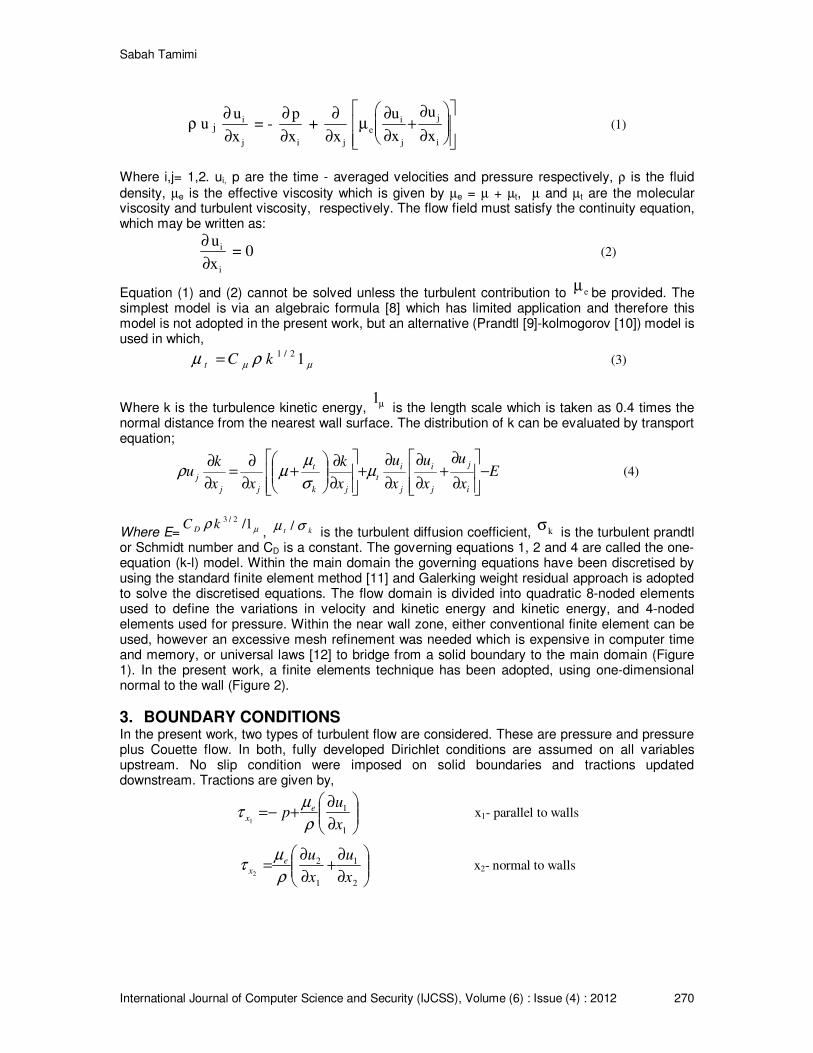
The investigation of this paper is related to steady - state incompressible two dimensional turbulent flow of a Newtonian viscous fluid with no body forces acting. For such a situation, the Navier-Stokes (N-S) equations associated with this type are,

Sabah Tamimi


ρ u j ∂

∂

u

x

i

j

= - ∂

∂

p

xi

+ ∂

∂x j

µ∂

∂

∂

∂e

i

j

j

i

u

x

u

x+

(1)

Where i,j= 1,2. ui, p are the time - averaged velocities and pressure respectively, ρ is the fluid

density, µe is the effective viscosity which is given by µe = µ + µt, µ and µt are the molecular viscosity and turbulent viscosity, respectively. The flow field must satisfy the continuity equation, which may be written as:

∂

∂

u

x

i

i

= 0 (2)

Equation (1) and (2) cannot be solved unless the turbulent contribution to µ e be provided. The

simplest model is via an algebraic formula [8] which has limited application and therefore this model is not adopted in the present work, but an alternative (Prandtl [9]-kolmogorov [10]) model is used in which,

µµ ρµ 12/1

kCt = (3)

Where k is the turbulence kinetic energy, 1µ is the length scale which is taken as 0.4 times the

normal distance from the nearest wall surface. The distribution of k can be evaluated by transport equation;

Ex

u

x

u

x

u

x

k

xx

ku

i

j

j

i

j

i

t

jk

t

jj

j−

∂

∂+

∂

∂

∂

∂+

∂

∂

+

∂

∂=

∂

∂µ

σ

µµρ (4)

Where E= µρ 1/2/3kC D , kt σµ /

is the turbulent diffusion coefficient, σk is the turbulent prandtl

or Schmidt number and CD is a constant. The governing equations 1, 2 and 4 are called the one-equation (k-l) model. Within the main domain the governing equations have been discretised by using the standard finite element method [11] and Galerking weight residual approach is adopted to solve the discretised equations. The flow domain is divided into quadratic 8-noded elements used to define the variations in velocity and kinetic energy and kinetic energy, and 4-noded elements used for pressure. Within the near wall zone, either conventional finite element can be used, however an excessive mesh refinement was needed which is expensive in computer time and memory, or universal laws [12] to bridge from a solid boundary to the main domain (Figure 1). In the present work, a finite elements technique has been adopted, using one-dimensional normal to the wall (Figure 2).

3. BOUNDARY CONDITIONS In the present work, two types of turbulent flow are considered. These are pressure and pressure plus Couette flow. In both, fully developed Dirichlet conditions are assumed on all variables upstream. No slip condition were imposed on solid boundaries and tractions updated downstream. Tractions are given by,

∂

∂+−=

1

1

1 x

up e

xρ

µτ x1- parallel to walls

∂

∂+

∂

∂=

2

1

1

2

2 x

u

x

uex

ρ

µτ x2- normal to walls

Sabah Tamimi


4. RESULTS AND DISCUSSION Two examples were used to validate the imposed wall element technique was tested and comparisons made with other accepted techniques and experimental results [14] when fully developed turbulent flow is considered in a parallel-sided duct of width D, which is taken as 1.0, and L is the channel length. Compatible fully developed velocity and kinetic energy profiles were imposed as initial upstream values and outlet values from the previous iteration used as new approximation to the values at the inlet until a converged condition is satisfied. Different Reynolds number based upon the width of the channel of 12.000, 50.000 and 70.000 were considered. The first example was concerned with an analysis of pressure flow where both walls of the channel are fixed. Figure 3 shows convergent velocity profiles at the outlet which clearly shows that the velocity values obtained by universal profiles have some discrepancy from those obtained from the advocated technique. Figures 4 shows the results obtained from the adoption of the presently advocated technique exhibits excellent agreement with the correct solution which resulted from the complete mapping. These are, superior to those obtained using universal laws. Figure 5 shows excellent agreement between the imposed technique and experimental results [14]. Figure 6 refer to the kinetic energy, which prove once more, the “correct” values are remarkably close to those obtained from the proposed technique. The next stage was concerned with the validation of the wall element technique in an extended near wall zone when the interface located at 0.48D and 0.47D from the symmetric line as shown in Figures 7-8. These figures show the downstream velocity and kinetic energy. Obviously the results obtained from the adoption of 1-D elements in one direction is still the most advantageous owing to the number of elements used in the near wall zone. The second example was concerned with an analysis of combining pressure and Couette flow, with the lower surface stationary and upper surface moving at a constant speed. Fully developed turbulent velocity profiles and turbulent kinetic energy distribution were obtained and presented in Figure 9 and 10, respectively, these show comparisons with universal laws and experimental results [14]. As conclusion, the validity of the wall element technique has been tested and approved previously [15-16]. In the present work, this validity has been tested again and approved again that the location of the near wall zone limit does not seem to affect the values of the pertinent variables. This is a distinct advantage over the universal law approach where strict limits must be placed on the location the interface, and once more, the results obtained from the adoption of the wall element technique are significantly better than those obtained using the universal laws, and compare favorably with experimental results.

FIGURE 1: Boundary conditions when the mesh is terminated at small distance away from the wall.

Sabah Tamimi


FIGURE 2: One-dimensional elements in one-direction normal to the wall used in the N.W.Z.

FIGURE 3: Turbulent velocity profiles for fully-developed flow, at flow, 8D downstream, L=8D, Re=50.000.

FIGURE 4: Turbulent velocity profiles for fully-developed at 8D downstream, L=8D, Re=12.000.

Sabah Tamimi


FIGURE 5: Turbulent velocity profiles for fully-developed flow, at 8D downstream, L=8D, Re=50.000.

FIGURE 6: Kinetic energy profiles for fully-developed turbulent flow, at 8D downstream, L=8D, Re=12.000.

FIGURE 7: Downstream fully developed velocity profiles for turbulent flow when the N.W.Z. is extended up

to 0.47D.

Sabah Tamimi


FIGURE 8: Downstream fully-developed kinetic energy profiles for turbulent flow when the N.W.Z. is

extended up to 0.47D.

FIGURE 9: Velocity profiles for fully-developed for turbulent flow with fixed lower surface and moving upper

surface, Re=70.000.

FIGURE 10: Fully-developed kinetic energy profiles for turbulent flow with fixed lower surface and moving

upper surface Re=70.000.

Sabah Tamimi


5. CONCLUSIONS The utilization of empirical universal laws is not valid since these laws are only really applicable for certain unidimensional flow regimes, and the general use of 2-D elements up to the wall is not economically viable. Therefore to avoid such an excessive refinement, these methods have been replaced by introducing a wall element technique, based on the use of the finite element methods which has shown an excellent results, when the fully-developed flow considered for both types of flow pressure and combination of pressure and Couette. Again, the validation of the wall element technique in an extended near wall zone has shown more advantages comparing to the use of universal laws. Therefore, the imposed technique can be used with confidence for fully-developed turbulent flow.

6. REFERENCES [1] C.L. Wiginton and C. Dalton, “Incompressible laminar flow in the entrance region of a

rectangular duct”, J. Apple. Mech., vol. 37, 1970, pp. 854-856.

[2] E.M. Sparrow, C.W. Hixoin, and G. Shavit, “Experiments on laminar flow development in ractangular duct”, J. Basic Eng., vol. 89, 1967, pp. 116-124.

[3] D.M. Hawken, H.R. Tamaddon-Jahromi, P. Townsend and M. F. Webster, “A Taylor-Galerkin based algorithm for viscous incompressible flow”, Int. Journal Num. Meth. Fluids, 1990.

[4] A.K. Mehrotra, and G.S. Patience, “Unified Entry Length for Newtonian and power law fluids in Laminar pipe flow”, J. Chem. Eng., vol. 68, 1990, pp.529-533.

[5] B.E. Launder, and N. Shima, “Second moment closure for near wall sublayer: Development and Application”, AIAA Journal, vol. 27, 1989, pp. 1319-1325.

[6] Haroutunian, and S. Engelman, “On modeling wall-bound turbulent flows using specialized

near-wall finite elements and the standard k-ε turbulent model”, Advances in Num. simulation of Turbulent flows, ASME, vol. 117, 1991, pp. 97-105.

[7] T. Graft, A. Gerasimov, H. Lacovides, B. Launder, “Progress in the generalization of wall-function treatments”, Int. Journal for heat and fluid flow, 2002, pp. 148-160.

[8] B.E. Launder, and D.B. Spalding, “Lectures in mathematical models of turbulence”, Academic Press, 1972.

[9] L. Prandtl, “Uber ein neues forelsystem fur die ausgebildete turbulenze”, Nachr. Akad. Der wissenschafft, Gottingesn, 1945.

[10] A.H. Kolmogrov, “Equations of turblent motion of an incompressible fluid”, IZV Akad Nauk, SSSR Ser. Phys, vol. 1-2, 1942, pp. 56-58.

[11] C. Taylor, and T.G. Hughes, “Finite element programming of the Navier-Stokes equation”, Pineridge press, 1981.

[12] T.J. Davies, “Turbulent phenomena”, Academic Press, 1972.

[13] G.E. Schneider, G.D. Raithby, and M. Kovanovich, “Finite element analysis of incompressible fluid flows incorporating equal order pressure and velocity interpolation”, Proc. Int. Conf. Num. Meth. in laminar and turbulent flow, Pentech Press, London, 1978, pp. 89-102.

Sabah Tamimi


[14] U.S.L. Nayak, and S.J. Stevens, “An experimental study of the flow in the annular gap between a long vehicle and a low close-fitting tunnel”, Report: Dept. of Technology, Loughborough University of Technology, 1973.

[15] Sabah Tamimi,” Representation of Variables of Confined Turbulent Flow in a Region Close to the Wall”, 12

th WSEAS International Conference on Applied Computer Science (ACS 12),

ISSN: 1790-5109, Singapore, 2012pp. 70-74.

[16] Sabah Tamimi, “Validation of Wall Element Technique of Turbulent Flow “, GSTF Int. Journal on Computing, ISSN: 2010-2283, Volume 2, No. 1, 2012, pp.177-181.

flow modeling based wall element technique

Education