Flow Characteristics and Energy Potentialin Tsugaru Strait toward Tide and Sea

Current Power Generation

by Makoto MIYATAKE

Institute of National Colleges of Technology,　　　　 Hakodate National College of Technology

Department of Civil Engineering,Hakodate National College of Technology

　 Backgrounds 　Basic message

Previous Qualitative Knowledge

The seasonal water flow characteristics are one of important factors that need to consider for power generation in Tsugaru Strait.

The seasonal characteristics of water flow across Tsugaru Strait has been known, that is dominated by both tide and ocean current.

The interaction mechanism in-depth of tide and ocean current in four seasons has not been well understood.

View of Tsugaru Strait during Winter Storm Season

OpenHydro and EDF (France):16m diameter ×42MW each35 m water depthelectricity for 4000 homes

To clarify the current interaction mechanism relationship between tide and ocean current by using the numerical modeling after reproducing the observation results accurately.

　 Objectives　

To investigate the variation characteristics of tide and ocean current through field observations of four seasons.

To estimate the energy potential based on the results of both field observations and numerical simulations.

20

25

303540455055606570

75

St.1

N

Toward Hakodate

ShiokubiHeadland

Hakodate City

Field Observations Setup　

Transmission Frequency 300kHz

MaximumSetup Depth 260m

Maximum Thickness of Layer

0.2m~16.0m

MaximumNumber of Layer 128

contents spec

Specifications of ADCP

ObservationPeriods

Spring 18th/3/2013~18th/4/2013(31days)Summer 31st/7/2013~4th/9/2013(35days)Autumn 19th/10/2013~4th/12/2013(45days)Winter 4th/12/2013~20th/1/2014(47days)

ObservationLayers

Upper 23.3m from sea bottomMiddle 12.2m from sea bottomBottom 3.2m from sea bottom

ObservationTime Intervals 60min.(Obs. Duration 40min., Sampling 1s.)

Observation Site and Method

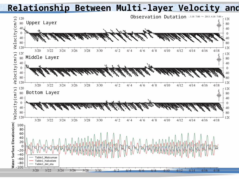
Relationship Between Multi-layer Velocity and Tide (Spring)　Ve

loci

ty(c

m/s

)Ve

loci

ty(c

m/s

)Ve

loci

ty(c

m/s

)

Upper Layer

Middle Layer

Bottom Layer

Observation Dutation

Normalized Cross-Correlation Function　

Upper LayerMiddle LayerBottom Layer

Nor

mal

ized

Cros

s-Co

rrel

ation

Fun

ction

Velo

city

(m/s

)

Time Lag(hr)

Tide Difference(cm)

(a) Relationship between Cross-Correlation and Time Lag

(b) Correlation of Tide Difference and Flow Velocity including 3hr Lags

UpperMiddleBottom

Normalized Cross-Correlation Function　

Frequency(Hz)

Pow

er S

pect

rum

(cm

2 sec

)

Tidal Current Ellipses of Principal Four Tidal Components

upper

middle

bottom

upper

middle

bottom

upper

middle

bottom

K1 O1 M2

S2

upper

middle

bottom

upper

middle

bottom

Composition

Dep

th(m

)

Dep

th(m

)D

epth

(m)

Dep

th(m

)

Dep

th(m

)

Water D

epth [m]

Longitude [deg]La

titud

e [d

eg]

50m

100m

300m

200m

Computation Range E140 - E141.383, N41.183 - N41.833

Mesh Scale（ Dlon. x Dlat.）

30sec x 30sec

Mesh Scale（ Vertical） 1.0m--15.0m

Time Step 10sec

Bottom Friction Slip-Boundary Condition

Start Time 15th/March 2013 00:00 (UTC)

Case # 1 2 3

Tidal Current

Tidal Current Velocity as Inflow Boundary Condition Given from TPXO7.2. ―

Ocean Current ―

Ocean Current Velocity as Inflow Boundary Condition Given from JAMSTEC FRA-JCOPE2

Numerical Simulations for Water Current

Specifications of CalculationComputation Area

Computation Cases

0

2

V

FVV

Dt

D

MITgcm(MIT General Circulation Model )

Same as Spring Obs.

Comparison Numerical Result with Observation Data

upper

middle

bottom

upper

middle

bottom

upper

middle

bottom

K1 O1 M2

S2

upper

middle

bottom

upper

middle

bottom

Composition

Dep

th(m

)

Dep

th(m

)D

epth

(m)

Dep

th(m

)

Dep

th(m

)

Orbit Radius [m

/s]

Longitude [deg]

Latit

ude

[deg

]

O1 1m/s

Orbit Radius [m

/s]

Longitude [deg]

Latit

ude

[deg

]

K1 1m/s

Orbit Radius [m

/s]

Longitude [deg]

Latit

ude

[deg

]

M2 1m/s

Orbit Radius [m

/s]

Longitude [deg]

Latit

ude

[deg

]

S2 1m/s

Black color： anticlockwise， Pink Color： clockwiseTidal Current Ellipse Distribution(Case 1; tidal current only)

Orbit Radius [m

/s]

Longitude [deg]

Latit

ude

[deg

]

O1 1m/s

Orbit Radius [m

/s]

Longitude [deg]

Latit

ude

[deg

]

K1 1m/s

Orbit Radius [m

/s]

Longitude [deg]

Latit

ude

[deg

]

M2 1m/s

Orbit Radius [m

/s]

Longitude [deg]

Latit

ude

[deg

]

S2 1m/s

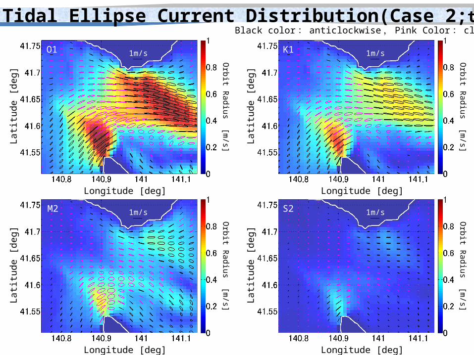
Tidal Ellipse Current Distribution(Case 2;tidal+ocean current)Black color： anticlockwise， Pink Color： clockwise

residual current velocity [m/s]

Longitude [deg]

Latit

ude

[deg

]

1m/s

residual current velocity [m/s]

Longitude [deg]

1m/s

Case 1

Case 3

residual current velocity [m/s]

Longitude [deg]

Latit

ude

[deg

]

1m/sCase 2

Latit

ude

[deg

]

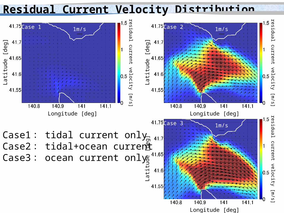
Residual Current Velocity Distribution

Case1： tidal current onlyCase2： tidal+ocean currentCase3： ocean current only

Density of Energy [kW

/m2]

Longitude [deg]

Latit

ude

[deg

]D

ensity of Energy [kW/m

2]

Longitude [deg]

Latit

ude

[deg

]D

ensity of Energy [kW/m

2]

Longitude [deg]

Latit

ude

[deg

]D

ensity of Energy [kW/m

2]

Longitude [deg]

Latit

ude

[deg

]

Case 1Case 1

Case 2Case 2

Depth Averaged Energy Potential Distribution

Duration average

Duration maximum

Duration average

Duration maximum

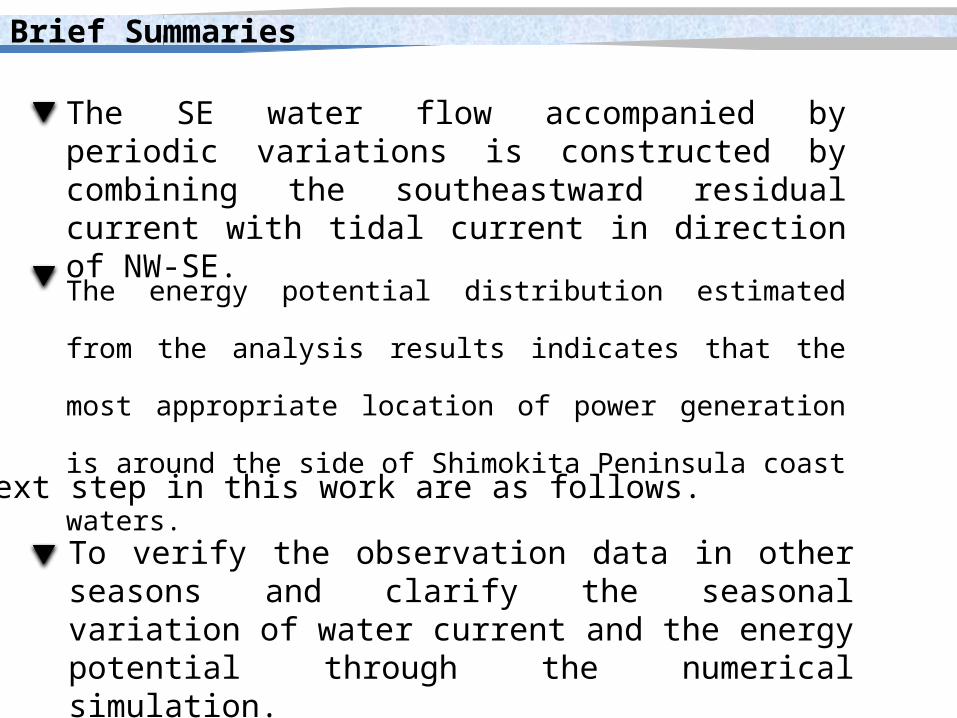
Brief Summaries

The SE water flow accompanied by periodic variations is constructed by combining the southeastward residual current with tidal current in direction of NW-SE.

The next step in this work are as follows.

The energy potential distribution estimated from the analysis results

indicates that the most appropriate location of power generation is

around the side of Shimokita Peninsula coast waters.

To verify the observation data in other seasons and clarify the seasonal variation of water current and the energy potential through the numerical simulation.