flexible priors for deep hierarchies - stanford...
TRANSCRIPT

Flexible Priors for Deep Hierarchies
Jacob Steinhardt
Wednesday, November 9, 2011

Hierarchical Modeling• many data are well-modeled by an
underlying tree
Wednesday, November 9, 2011

Hierarchical Modeling• many data are well-modeled by an
underlying tree
!"#$%&%'%&()*+)$(,+-.%&&)$/0)1%&#)$2-$3)+)4%(+#.5$6%+%$.%!"#$
%&'()(*+,-./,0,1.232/3-4-526734-0381-,9
.23:#;<:$4=>.-45.>,1.23,+-.%%/#$7&-6("%2)(#-$)89.)/%41-6:.#%$.%&1-,9:<<:?#@@:(A23B,54=C74-6D4>-3>.-/5.38.,.23!;#@@.3-9>.24.,55C--38/09,-3.240!B38,5C930.>;6/378/0E45,-+C>,1#($F
D,-8>(A23734-0382/3-4-526;,1D2/52,0764+,-./,0/>/77C>.-4.38;5,0.4/0>GH.,+/5>(I,.3.24..23!+4-493.3-/>!J384.4>94773-B47C3;.,+-,B/834-34>,04=76>/K38.,+/52/3-4-526D/.2.23>/E0/!540.7674-E3-5,-+C>(
LM*24>=330>2,D0.,6/378E,,8+-38/5./B3+3-1,-94053-374./B3.,5,9+3./0E
C0/E-49740EC4E39,837>;408/.24>47>,=3304-EC38.24..23.,+/5N=4>3840476N
>/>+-,B/838=6LM*-3+-3>30.>4OC47/.4./B3/9+-,B3930.,05,9+3./0E740EC4E39,837>PQ73/3.47(#@@$=R'-/1!.2>408S.36B->#@@HT(A2C>LM*+-,B/83>404.C-47+,/0.,15,9+4-/>,0(A23-34-3>3B3-47/>>C3>.24.9C>.=3=,-03/09/08/05,9+4-/0E2LM*.,LM*(
%/->.;/0LM*.230C9=3-,1.,+/5>/>4!J38+4-493.3-;40849,837>3735./,0
U,C-047,1.23*VF;W,7(G!;I,(#;*-./573!;XC=7/54./,084.3"U40C4-6#@:@(
Wednesday, November 9, 2011

Hierarchical Modeling• many data are well-modeled by an
underlying tree
Figure 3: These figures show a subset of the tree learned from the 50,000 CIFAR-100 images. The top tree only
shows nodes for which there were at least 250 images. The ten shown at each node are those with the highest
probability under the node’s distribution. The second row shows three expanded views of subtrees, with nodes
that have at least 50 images. Detailed views of portions of these subtrees are shown in the third row.
Selecting a Single Tree We have so far described a procedure for generating posterior samples
from the tree structures and associated stick-breaking processes. If our objective is to find a single
tree, however, samples from the posterior distribution are unsatisfying. Following [17], we report a
best single tree structure over the data by choosing the sample from our Markov chain that has the
highest complete-data likelihood p({xn, �n}Nn=1 | {ν�}, {ψ�},α0,λ, γ).
5 Hierarchical Clustering of Images
We applied our model and MCMC inference to the problem of hierarchically clustering the CIFAR-
100 image data set1. These data are a labeled subset of the 80 million tiny images data [22]
with 50,000 32×32 color images. We did not use the labels in our clustering. We modeled the
images via 256-dimensional binary features that had been previously extracted from each image
(i.e., xn ∈ {0, 1}256) using a deep neural network that had been trained for an image retrieval task
[23]. We used a factored Bernoulli likelihood at each node, parameterized by a latent 256-dimensional
real vector (i.e., θ� ∈ R256) that was transformed component-wise via the logistic function:
f(xn | θ�) =256�
d=1
�1 + exp{−θ(d)� }
�−x(d)n
�1 + exp{θ(d)� }
�1−x(d)n
.
The prior over the parameters of a child node was Gaussian with its parent’s value as the mean.
The covariance of the prior (Λ in Section 3) was diagonal and inferred as part of the Markov chain.
We placed independent Uni(0.01, 1) priors on the elements of the diagonal. To efficiently learn the
node parameters, we used Hamiltonian (hybrid) Monte Carlo (HMC) [24], taking 25 leapfrog HMC
steps, with a randomized step size. We occasionally interleaved a slice sampling move for robustness.
1http://www.cs.utoronto.ca/˜kriz/cifar.html
6
Wednesday, November 9, 2011

Hierarchical Modeling• many data are well-modeled by an
underlying tree
00.10.2[Armenian] Armenian (Eastern)[Armenian] Armenian (Western)[Indic] Bengali[Indic] Marathi[Indic] Maithili[Iranian] Ossetic[Indic] Nepali[Indic] Sinhala[Indic] Kashmiri[Indic] Hindi[Indic] Panjabi[Iranian] Pashto[Slavic] Czech[Baltic] Latvian[Baltic] Lithuanian[Slavic] Russian[Slavic] Ukrainian[Slavic] Serbian−Croatian[Slavic] Slovene[Slavic] Polish[Albanian] Albanian[Romance] Catalan[Romance] Italian[Romance] Portuguese[Romance] Romanian[Slavic] Bulgarian[Greek] Greek (Modern)[Romance] Spanish[Germanic] Danish[Germanic] Norwegian[Germanic] Swedish[Germanic] Icelandic[Germanic] English[Germanic] Dutch[Germanic] German[Romance] French[Iranian] Kurdish (Central)[Iranian] Persian[Iranian] Tajik[Celtic] Breton[Celtic] Cornish[Celtic] Welsh[Celtic] Gaelic (Scots)[Celtic] Irish
(a) Coalescent for a subset of Indo-European lan-guages from WALS.
0.1 0.2 0.3 0.4 0.572
74
76
78
80
82
CoalescentNeighborAgglomerativePPCA
(b) Data restoration on WALS. Y-axis is accuracy;X-axis is percentage of data set used in experiments.At 10%, there are N = 215 languages, H = 14features and p = 94% observed data; at 20%, N =430, H = 28 and p = 80%; at 30%: N = 645,H = 42 and p = 66%; at 40%: N = 860, H =56 and p = 53%; at 50%: N = 1075, H = 70and p = 43%. Results are averaged over five foldswith a different 5% hidden each time. (We also trieda “mode” prediction, but its performance is in the60% range in all cases, and is not depicted.)
Figure 3: Results of the phylolinguistics experiments.
LLR (t) Top Words Top Authors (# papers)32.7 (-2.71) bifurcation attractors hopfield network saddle Mjolsness (9) Saad (9) Ruppin (8) Coolen (7)
0.106 (-3.77) voltage model cells neurons neuron Koch (30) Sejnowski (22) Bower (11) Dayan (10)83.8 (-2.02) chip circuit voltage vlsi transistor Koch (12) Alspector (6) Lazzaro (6) Murray (6)
140.0 (-2.43) spike ocular cells firing stimulus Sejnowski (22) Koch (18) Bower (11) Dayan (10)2.48 (-3.66) data model learning algorithm training Jordan (17) Hinton (16) Williams (14) Tresp (13)31.3 (-2.76) infomax image ica images kurtosis Hinton (12) Sejnowski (10) Amari (7) Zemel (7)31.6 (-2.83) data training regression learning model Jordan (16) Tresp (13) Smola (11) Moody (10)39.5 (-2.46) critic policy reinforcement agent controller Singh (15) Barto (10) Sutton (8) Sanger (7)23.0 (-3.03) network training units hidden input Mozer (14) Lippmann (11) Giles (10) Bengio (9)
Table 3: Nine clusters discovered in NIPS abstracts data.
NIPS. We applied Greedy-Rate1 to all NIPS abstracts through NIPS12 (1740, total). The data waspreprocessed so that only words occuring in at least 100 abstracts were retained. The word countswere then converted to binary. We performed one iteration of hyperparameter re-estimation. Inthe supplemental material, we depict the top levels of the coalescent tree. Here, we use the tree togenerate a flat clustering. To do so, we use the log likelihood ratio at each branch in the coalescentto determine if a split should occur. If the log likelihood ratio is greater than zero, we break thebranch; otherwise, we recurse down. On the NIPS abstracts, this leads to nine clusters, depictedin Table 3. Note that clusters two and three are quite similar—had we used a slighly higher loglikelihood ratio, they would have been merged (the LLR for cluster 2 was only 0.105). Note thatthe clustering is able to tease apart Bayesian learning (cluster 5) and non-bayesian learning (cluster7)—both of which have Mike Jordan as their top author!
6 Discussion
We described a new model for Bayesian agglomerative clustering. We used Kingman’s coalescentas our prior over trees, and derived efficient and easily implementable greedy and SMC inferencealgorithms for the model. We showed empirically that our model gives better performance than other
Wednesday, November 9, 2011

Hierarchical Modeling
Wednesday, November 9, 2011

Hierarchical Modeling
• advantages of hierarchical modeling:
Wednesday, November 9, 2011

Hierarchical Modeling
• advantages of hierarchical modeling:
• captures both broad and specific trends
Wednesday, November 9, 2011

Hierarchical Modeling
• advantages of hierarchical modeling:
• captures both broad and specific trends
• facilitates transfer learning
Wednesday, November 9, 2011

Hierarchical Modeling
• advantages of hierarchical modeling:
• captures both broad and specific trends
• facilitates transfer learning
• issues:
Wednesday, November 9, 2011

Hierarchical Modeling
• advantages of hierarchical modeling:
• captures both broad and specific trends
• facilitates transfer learning
• issues:
• the underlying tree may not be known
Wednesday, November 9, 2011

Hierarchical Modeling
• advantages of hierarchical modeling:
• captures both broad and specific trends
• facilitates transfer learning
• issues:
• the underlying tree may not be known
• predictions in deep hierarchies can be strongly influenced by the prior
Wednesday, November 9, 2011

Learning the Tree
Wednesday, November 9, 2011

Learning the Tree
• major approaches for choosing a tree:
Wednesday, November 9, 2011
Learning the Tree
• major approaches for choosing a tree:
• agglomerative clustering
Wednesday, November 9, 2011

Learning the Tree
• major approaches for choosing a tree:
• agglomerative clustering
• Bayesian methods (place prior over trees)
Wednesday, November 9, 2011

Learning the Tree
• major approaches for choosing a tree:
• agglomerative clustering
• Bayesian methods (place prior over trees)
• stochastic branching processes
Wednesday, November 9, 2011

Learning the Tree
• major approaches for choosing a tree:
• agglomerative clustering
• Bayesian methods (place prior over trees)
• stochastic branching processes
• nested random partitions
Wednesday, November 9, 2011

Agglomerative Clustering
• start with each datum in its own subtree
• iteratively merge subtrees based on a similarity metric
• issues:
• can’t add new data
• can’t form hierarchies over latent parameters
• difficult to incorporate structured domain knowledge
Wednesday, November 9, 2011

Stochastic Branching Processes
• fully Bayesian model
• data starts at top and branches based on an arrival process (Dirichlet diffusion trees)
• can also start at bottom and merge (Kingman coalescents)
Consider the tree of N = 4 data points in Figure 1.The probability of obtaining this tree structure andassociated divergence times is:
e−A(ta)Γ(1−β)Γ(2+α)
a(ta)Γ(1− β)
Γ(2 + α)
× e−A(ta)Γ(2−β)Γ(3+α)
1− β
2 + αe−[A(ta)−A(tb)]
Γ(1−β)Γ(2+α)
a(tb)Γ(1− β)
Γ(2 + α)
× e−A(ta)Γ(3−β)Γ(4+α)
α+ 2β
3 + α
The first data point does not contribute to the expres-sion. The second point contributes the first line: thefirst term results from not diverging between t = 0 andta, the second from diverging at ta. The third pointcontributes the second line: the first term comes fromnot diverging before time ta, the second from choosingthe branch leading towards the first point, the thirdterm comes from not diverging between times ta andtb, and the final term from diverging at time tb. Thefourth and final data point contributes the final line:the first term for not diverging before time ta and thesecond term for diverging at branch point a.
The component resulting from the divergence and datalocations for the tree in Figure 1 is
N(x1; 0,σ2)N(x2;xa,σ
2(1− ta))
×N(x3;xb,σ2(1− tb))N(x4;xa,σ
2(1− ta))
where each data point has contributed a term. We canrewrite this as:
N(xa; 0,σ2ta)N(xb;xa,σ
2(tb − ta))
×N(x1;xb,σ2(1− tb))×N(x2;xa,σ
2(1− ta))
×N(x3;xb,σ2(1− tb))N(x4;xa,σ
2(1− ta)) (5)
to see that there is a Gaussian term associated witheach branch in the tree.
3 Theory
Now we present some important properties of thePYDT generative process.
Lemma 1. The probability of generating a specific treestructure, divergence times, divergence locations andcorresponding data set is invariant to the ordering ofdata points.
Proof. The probability of a draw from the PYDT canbe decomposed into three components: the probabil-ity of the underlying tree structure, the probabilityof the divergence times given the tree structure, andthe probability of the divergence locations given thedivergence times. We will show that none of these
Figure 1: A sample from the Pitman-Yor DiffusionTree with N = 4 datapoints and a(t) = 1/(1− t),α =1,β = 0. Top: the location of the Brownian motionfor each of the four paths. Bottom: the correspondingtree structure. Each branch point corresponds to aninternal tree node.
components depend on the ordering of the data. Con-sider the tree T as a set of edges S(T ) each of whichwe will see contributes to the joint probability den-sity. The tree structure T contains the counts ofhow many datapoints traversed each edge. We de-note an edge by [ab] ∈ S(T ), which goes from nodea to node b with corresponding locations xa and xb
and divergence times ta and tb. Let m(b) be the num-ber of samples to have passed through b. Denote byS �(T ) = {[ab] ∈ S(T ) : m(b) ≥ 2} the set of all edgestraversed by m ≥ 2 samples (for divergence functionswhich ensure divergence before time 1 this is the setof all edges not connecting to leaf nodes).
Probability of the tree structure. For segment [ab], leti be the index of the sample which diverged to createthe branch point at b, thereby contributing a factor
a(tb)Γ(i− 1− β)
Γ(i+ α). (6)
Let the number of branches from b be Kb, and thenumber of samples which followed each branch be{nb
k : k ∈ [1 . . .Kb]}. The total number of datapoints
which traversed edge [ab] is m(b) =�Kb
j=1 nbk. It can
be shown (see Appendix A) that the factor associatedwith this branching structure for the data points afteri is
�Kb
k=3[α+ (k − 1)β]Γ(i+ α)�Kb
l=1 Γ(nbl − β)
Γ(i− 1 + β)Γ(m(b) + α)
Wednesday, November 9, 2011

Stochastic Branching Processes
• many nice properties
• infinitely exchangeable
• complexity of tree grows with the data
• latent parameters must undergo a continuous-time diffusion process
• unclear how to construct such a process for models over discrete data
Wednesday, November 9, 2011

Random Partitions
• stick-breaking process: a way to partition the unit interval into countably many masses π1,π2,...
• draw βk from Beta(1,γ)
• let πk = βk x (1-β1) ... (1-βk-1)
• the distribution over the πk is called a Dirichlet process
Wednesday, November 9, 2011

Random Partitions
• suppose {πk}k=1,...,∞ are drawn from a Dirichlet process
• for n=1,..,N, let Xn ~ Multinomial({πk})
• induces distribution over partitions of {1,...,N}
• given partition of {1,...,N}, add XN+1 to a part of size s with probability s/(N+γ) and to a new part with probability γ/(N+γ)
• Chinese restaurant processWednesday, November 9, 2011

Nested Random Partitions
• a tree is equivalent to a collection of nested partitions
• nested tree <=> nested random partitions
• partition at each node given by Chinese restaurant process
• issue: when to stop recursing?
Wednesday, November 9, 2011

Martingale Property
• martingale property: E[f(θchild) | θparent] = f(θparent)
• implies E[f(θv) | θu] = f(θu) for any ancestor u of v
• says that learning about a child does not change beliefs in expectation
Wednesday, November 9, 2011

Doob’s Theorem
Wednesday, November 9, 2011

Doob’s Theorem
• Let θ1, θ2,... be a sequence of random variables such that E[f(θn+1) | θn] = f(θn) and supn E[|θn|] < ∞.
Wednesday, November 9, 2011

Doob’s Theorem
• Let θ1, θ2,... be a sequence of random variables such that E[f(θn+1) | θn] = f(θn) and supn E[|θn|] < ∞.
• Then limn!∞f(θn) exists with probability 1.
Wednesday, November 9, 2011

Doob’s Theorem
• Let θ1, θ2,... be a sequence of random variables such that E[f(θn+1) | θn] = f(θn) and supn E[|θn|] < ∞.
• Then limn!∞f(θn) exists with probability 1.
• Intuition: each new random variable reveals more information about f(θ) until it is completely determined.
Wednesday, November 9, 2011

Doob’s Theorem
• Use Doob’s theorem to build infinitely deep hierarchy
• data associated with infinite paths v1,v2,... down the tree
• each datum drawn from distribution parameterized by limn f(θvn)
Wednesday, November 9, 2011

Doob’s Theorem
• all data have infinite depth
• can think of effective depth of a datum as first point where it is in a unique subtree
• effective depth is O(logN)
Wednesday, November 9, 2011

Letting the Complexity Grow with the DataManuscript under review by AISTATS 2012
Figure 2: Trees drawn from the prior of the model with N = 100 data points. At the top is the tree generatedby tree-structured stick breaking, and at the bottom is the tree generated by the nCRP. In both cases we used ahyper-parameter of γ = 1. For the stick breaking model, we further set α = 10 and λ = 1
2 (these are parametersthat do not exist in our model). Note that the tree generated by TSSB is very wide and shallow. A larger valueof α would fix this for N = 100, but increasing N would cause the problem to re-appear.
0 500 1000 1500 2000 2500 30000
5
10
15
20
25
number of data points
maxi
mum
depth
nCRPTSSB!10!0.5TSSB!20!1.0TSSB!50!0.5TSSB!100!0.8
0 500 1000 1500 2000 2500 30001
2
3
4
5
6
7
8
9
number of data points
ave
rage d
epth
nCRPTSSB!10!0.5TSSB!20!1.0TSSB!50!0.5TSSB!100!0.8
Figure 3: Tree depth versus number of data points. We drew a single tree from the prior for the nCRP as wellas for tree-structured stick-breaking, and computed both the maximum and average depth as more data wasadded to the tree. The above plots show that the depth of the nCRP increases with the amount of data, whereasthe depth of tree-structured stick-breaking (TSSB) quickly converges to a constant. The different curves for theTSSB model correspond to different settings of the hyperparameters α and λ.
Wednesday, November 9, 2011

Letting the Complexity Grow with the Data
Manuscript under review by AISTATS 2012
Figure 2: Trees drawn from the prior of the model with N = 100 data points. At the top is the tree generatedby tree-structured stick breaking, and at the bottom is the tree generated by the nCRP. In both cases we used ahyper-parameter of γ = 1. For the stick breaking model, we further set α = 10 and λ = 1
2 (these are parametersthat do not exist in our model). Note that the tree generated by TSSB is very wide and shallow. A larger valueof α would fix this for N = 100, but increasing N would cause the problem to re-appear.
0 500 1000 1500 2000 2500 30000
5
10
15
20
25
number of data points
maxi
mum
depth
nCRPTSSB!10!0.5TSSB!20!1.0TSSB!50!0.5TSSB!100!0.8
0 500 1000 1500 2000 2500 30001
2
3
4
5
6
7
8
9
number of data points
ave
rage d
epth
nCRPTSSB!10!0.5TSSB!20!1.0TSSB!50!0.5TSSB!100!0.8
Figure 3: Tree depth versus number of data points. We drew a single tree from the prior for the nCRP as wellas for tree-structured stick-breaking, and computed both the maximum and average depth as more data wasadded to the tree. The above plots show that the depth of the nCRP increases with the amount of data, whereasthe depth of tree-structured stick-breaking (TSSB) quickly converges to a constant. The different curves for theTSSB model correspond to different settings of the hyperparameters α and λ.
Wednesday, November 9, 2011

Hierarchical Beta Processes
Wednesday, November 9, 2011

Hierarchical Beta Processes
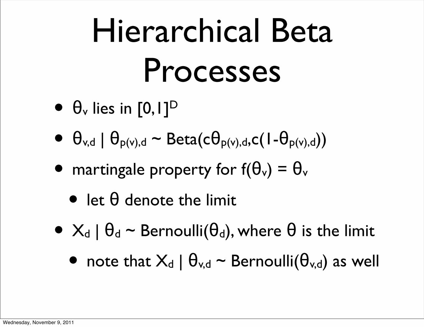
• θv lies in [0,1]D
Wednesday, November 9, 2011

Hierarchical Beta Processes
• θv lies in [0,1]D
• θv,d | θp(v),d ~ Beta(cθp(v),d,c(1-θp(v),d))
Wednesday, November 9, 2011

Hierarchical Beta Processes
• θv lies in [0,1]D
• θv,d | θp(v),d ~ Beta(cθp(v),d,c(1-θp(v),d))
• martingale property for f(θv) = θv
Wednesday, November 9, 2011

Hierarchical Beta Processes
• θv lies in [0,1]D
• θv,d | θp(v),d ~ Beta(cθp(v),d,c(1-θp(v),d))
• martingale property for f(θv) = θv
• let θ denote the limit
Wednesday, November 9, 2011

Hierarchical Beta Processes
• θv lies in [0,1]D
• θv,d | θp(v),d ~ Beta(cθp(v),d,c(1-θp(v),d))
• martingale property for f(θv) = θv
• let θ denote the limit
• Xd | θd ~ Bernoulli(θd), where θ is the limit
Wednesday, November 9, 2011
Hierarchical Beta Processes
• θv lies in [0,1]D
• θv,d | θp(v),d ~ Beta(cθp(v),d,c(1-θp(v),d))
• martingale property for f(θv) = θv
• let θ denote the limit
• Xd | θd ~ Bernoulli(θd), where θ is the limit
• note that Xd | θv,d ~ Bernoulli(θv,d) as well
Wednesday, November 9, 2011

Hierarchical Beta ProcessesManuscript under review by AISTATS 2012
Figure 4: Part of a sample from the incremental Gibbs sampler for our model applied to a hierarchical betaprocess. The latent parameters at internal nodes are represented by gray lines with white = 0, black = 1. Thenodes with thicker borders represent data. The complete tree is available in the supplementary material.
hierarchies due to general numerical issues with hier-archical Beta processes. The numerical issues occurwhen we are resampling the parameters of a node andone of the values of the children is very close to 0 or 1.If a child parameter is very close to 0, for instance, itactually matters for the likelihood whether the param-eter is equal to 10−10 or 10−50 (or even 10−1000). Sincewe cannot actually distinguish between these numberswith floating point arithmetic, this introduces innacu-racies in the posterior that push all of the parameterscloser to 0.5. To deal with this problem, we assumethat we cannot distinguish between numbers that areless than some distance � from 0 or 1. If we see sucha number, we treat it as having a censored value (soit appears as P[θ < �] or P[θ > 1 − �] in the likeli-hood). We then obtain a log-concave conditional den-sity, for which efficient sampling algorithms exist (Ley-dold, 2003).
Scalability If there are N data points, each with L
features, and the tree has depth D, then the time ittakes to add a data point is O(NL), the time it takes toremove a data point is O(L+D), and the time it takesto resample a single set of parameters is (amortized)O(L). The dominating operation is adding a node, soto make a Gibbs update for all data points will taketotal time O(N2L).
Results To demonstrate inference in our model, wecreated a data set of 53 stick figures determined bythe presence or absence of a set of 29 lines. We thenran incremental Gibbs sampling for 100 iterations withhyperparameters of γ = 1.0, c = 20.0. The output ofthe final sample is given in Figure 4.
5 Conclusion
We have presented an exchangeable prior over discretehierarchies that can flexibly increase its depth to ac-comodate new data. We have also implemented thisprior for a hierarchical beta process. Along the way,we identified a common model property — the martin-gale property — that has interesting and unexpectedconsequences in deep hierarchies.
This paper has focused on a general theoretical charac-terization of infinitely exchangeable distributions overtrees based on the Doob martingale convergence the-orem, on elucidating properties of deep hierarchicalbeta processes as an example of such models, and ondefining an efficient inference algorithm for such mod-els, which was demonstrated on a small binary dataset. A full experimental evaluation of nonparametricBayesian models for hierarchices is outside the scopeof this paper but clearly of interest.
Wednesday, November 9, 2011

Priors for Deep Hierarchies
• for HBP, θv,d converges to 0 or 1
• rate of convergence: tower of exponentials
• numerical issues + philosophically troubling
eeee
···
Wednesday, November 9, 2011

Priors for Deep Hierarchies
• inverse Wishart time-series
• Σn+1 | Σn ~ InvW(Σn)
• converges to 0 with probability 1
• becomes singular to numerical precision
• rate also given by tower of exponentials
Wednesday, November 9, 2011

Priors for Deep Hierarchies
• fundamental issues with iterated gamma distribution
• θn+1 | θn ~ Γ(θn)
• instead, do θn+1 | θn ~ cθn +dϕn
• ϕn ~ Γ(θn)
Wednesday, November 9, 2011

Priors for Deep Hierarchies
0 50 100 150 200 250 300 350 400 450 5000
0.1
0.2
0.3
0.4
0.5
0.6
0.7
0.8
depth
mass
kappa = 10.0, epsilon = 0.1
0 50 100 150 200 250 300 350 400 450 5000.06
0.07
0.08
0.09
0.1
0.11
0.12
0.13
depth
mass
proposed model
0 50 100 150 200 250 300 350 400 450 50010
!25
10!20
10!15
10!10
10!5
100
depth
mass
kappa = 10.0, epsilon = 0.1
1 2 3 4 5 6 7 810
!10
10!8
10!6
10!4
10!2
100
depth
mass
kappa = 10.0, epsilon = 0.0
Figure 1: Sampled values of the mass of an atom in a hierarchical Dirichlet process as a function
of depth. Top-left: a standard hierarchical Dirichlet process with κ = 10.0, � = 0.1. Note that
the mass spends a lot of time near zero. Top-right: our first proposed change to the hierarchical
Dirichlet process. Note that the mass now converges to a nonzero value. Bottom-left: the top-left
graph on a semilogarithmic scale, which demonstrates that the mass regularly drops to values below
10−7. Bottom-right: a demonstration of what happens if we just use the model θc ∼ DP(κθv) (in
other words, if we set � to zero). We only show up to a depth of 8 because at higher depths the mass
is smaller than 10−308and therefore rounded to 0 on a computer.
processes with a suitable parameterization of the Pitman-Yor process (Gasthaus and Teh, 2011),
such that the parameters converge to a single atom at a controlled rate. This parameterization has
the further advantage that it is the marginal distribution of a continuous-time stochastic process, and
can therefore be incorporated into the framework of Dirichlet diffusion trees (Neal, 2003; Knowles
and Ghahramani, 2011).
ReferencesRyan P. Adams, Zoubin Ghahramani, and Michael I. Jordan. Tree-structured stick breaking for
hierarchical data. Advanced in Neural Information Processing Systems, 23, 2010.
David M. Blei, Thomas L. Griffiths, and Michael I. Jordan. The nested chinese restaurant process
and bayesian nonparametric inference of topic hierarchies. Journal of the ACM, 57(2), Jan 2010.
Jan Gasthaus and Yee Whye Teh. Improvements to the sequence memoizer. Advances in NeuralInformation Processing Systems, 2011.
David Knowles and Zoubin Ghahramani. Pitman-yor diffusion trees. Uncertainty in Artificial Intel-ligence, 27, 2011.
R M Neal. Density modeling and clustering using dirichlet diffusion trees. In Bayesian Statistics 7,
pages 619–629, 2003.
Y W Teh, M I Jordan, M J Beal, and D M Blei. Hierarchical dirichlet processes. Technical Report
653, 2004.
Romain Thibaux. Nonparametric Bayesian Models for Machine Learning. PhD thesis, University
of California, Berkeley, 2008.
Romain Thibaux and Michael I. Jordan. Hierarchical beta processes and the indian buffet process.
AISTATS, 2007.
2
Wednesday, November 9, 2011