flexible multibody dynamic modeling and … · rhex hexapod robot with half circular ... and are...
TRANSCRIPT
FLEXIBLE MULTIBODY DYNAMIC MODELING AND SIMULATION OF RHEX HEXAPOD ROBOT WITH HALF CIRCULAR COMPLIANT LEGS
A THESIS SUBMITTED TO THE GRADUATE SCHOOL OF NATURAL AND APPLIED SCIENCES
OF MIDDLE EAST TECHNICAL UNIVERSITY
BY
GÖKHAN ORAL
IN PARTIAL FULFILLMENT OF THE REQUIREMENTS FOR
THE DEGREE OF MASTER OF SCIENCE IN
MECHANICAL ENGINEERING
NOVEMBER 2008
b
Approval of the thesis:
FLEXIBLE MULTIBODY DYNAMIC MODELING AND SIMULATION OF RHEX HEXAPOD ROBOT WITH HALF CIRCULAR COMPLIANT LEGS
submitted by GÖKHAN ORAL in partial fulfillment of the requirements for the degree of Master of Science in Mechanical Engineering Department, Middle East Technical University by, Prof. Dr. Canan Özgen Dean, Graduate School of Natural and Applied Sciences Prof. Dr. Süha Oral Head of Department, Mechanical Engineering Assist. Prof. Dr. Yiğit Yazıcıoğlu Supervisor, Mechanical Engineering Dept., METU Assist. Prof. Dr. Afşar Saranlı Co supervisor, Electrical and Electronics Eng. Dept., METU Examining Committee Members: Prof. Dr. Samim Ünlüsoy Mechanical Engineering Dept., METU Assist. Prof. Dr. Yiğit Yazıcıoğlu Mechanical Engineering Dept., METU Prof. Dr. Kemal İder Mechanical Engineering Dept., METU Assist. Prof. Dr. Buğra Koku Mechanical Engineering Dept., METU Assist. Prof. Dr.. Veysel Gazi Electrical Engineering Dept., TOBB UNIVERSITY OF ECONOMICS AND TECHNOLOGY
Date: Nov 24, 2008

iii
I hereby declare that all information in this document has been obtained and presented in accordance with academic rules and ethical conduct. I also declare that, as required by these rules and conduct, I have fully cited and referenced all material and results that are not original to this work.
Name, Last name : Gökhan Oral
Signature :
iv
ABSTRACT
FLEXIBLE MULTIBODY DYNAMIC MODELING AND SIMULATION OF RHEX HEXAPOD ROBOT WITH HALF
CIRCULAR COMPLIANT LEGS
Oral, Gökhan
M. S. in Department of Mechanical Engineering
Supervisor: Assist. Prof. Dr. Yiğit Yazıcıoğlu
Co-Supervisor: Assist. Prof. Dr. Afşar Saranlı
November, 2008,130 pages
The focus of interest in this study is the RHex robot, which is a hexapod robot
that is capable of locomotion over rugged, fractured terrain through statically
and dynamically stable gaits while stability of locomotion is preserved. RHex
is primarily a research platform that is based on over five years of previous
research. The purpose of the study is to build a virtual prototype of RHex
robot in order to simulate different behavior without manufacturing expensive
prototypes. The virtual prototype is modeled in MSC ADAMS software which
is a very useful program to simulate flexible multibody dynamical systems.
The flexible half circular legs are modeled in a finite element program (MSC
NASTRAN) and are embedded in the main model. Finally a closed loop
control mechanism is built in MATLAB to be able to simulate real
autonomous RHex robot. The interaction of MATLAB and MSC ADAMS
softwares is studied.
Keywords: Multibody Dynamics Simulation, Finite Element Analysis, Flexible
Multibody Dynamic Modeling,

v
ÖZ
YARIM DAİRE ŞEKLİNDEKİ ESNEK ALTI BACAKLI RHEX ROBOTUNUN ESNEK ÇOK GÖVDELİ DİNAMİK
MODELLENMESİ VE SİMULASYONU
Oral, Gökhan
Yüksek Lisans Makine Mühendisliği Bölümü
Tez Yöneticisi: Y. Doç. Dr. Yiğit Yazıcıoğlu
Ortak Tez Yöneticisi: Assist. Prof. Dr. Afşar Saranlı
Kasım, 2008, 130 sayfa
Yarım daire şeklindeki esnek altı bacaklı Rhex robotu bozuk yüzeylerde
dinamik stabilitesini koruyarak saniyede boyunun birkaç katı hızda
ilerleyebilmektedir. Bu tezin amacı esnek çok gövdeli bir yapıya sahip olan
Rhex robotunun dinamik modelinin oluşturulmasıdır. MSC ADAMS programı
robotun ana dinamik modelinin oluşturulmasında kullanılmıştır. Esnek
bacaklar sonlu eleman analizi programı olan MSC NASTRAN ile çözülmüş ve
ana modele eklenmiştir. En son aşama olarak oluşturulan dinamik modelin
MATLAB kontrol programı ile entegrasyonu tamamlanmış böylece otonom
davranış sergileyebilen RHex robotunun tam modeli çıkarılmıştır. Prototip
üreterek farklı davranışları ve farklı özellikteki parçaları robot üzerinde
denemek çoğu zaman pahalı ve çok zaman gerektiren bir süreç olmuştur. Bu
tezde karmaşık çok gövdeli altı bacaklı robot RHex’in sanal bir modeli
oluşturulmuştur.
Anahtar kelimeler: Çok gövdeli dinamik modelleme, Sonlu eleman analizi,
esnek çok gövdeli dinamik modelleme

vi
ACKNOWLEDGEMENTS
I deeply thank to whom has participated within this study.
vii
TABLE OF CONTENTS
ABSTRACT .................................................................................................... iv
ÖZ ................................................................................................................... v
ACKNOWLEDGEMENTS .............................................................................. vi
CHAPTERS
1. INTRODUCTION ...................................................................................... 1
1.1. Wheeled and Tracked Robots ............................................................. 4
1.2. Legged Robots .................................................................................... 5
1.3. Present Day Legged Robots ............................................................... 9
1.3.1. Monopod Robots .......................................................................... 9
1.3.2. Biped Robots .............................................................................. 13
1.3.3. Quadruped Robots...................................................................... 16
1.3.4. Hexapod Robots ......................................................................... 19
1.4. Flexible Multibody Dynamic Simulation ............................................. 22
2. MECHANICAL DESIGN OF RHEX ......................................................... 28
2.1 Overall Description of the Design ....................................................... 28
2.2. Crash Frame ..................................................................................... 30
2.3. Base Frame ....................................................................................... 31
2.4. Motor mounting parts ........................................................................ 34
2.5. The Flexible Legs .............................................................................. 36
2.6. Inner Mounting Parts ......................................................................... 37
2.6.1. Motor Driver Board Holder .......................................................... 38
2.6.2 Side Supports .............................................................................. 39
2.6.3 PC104 Housing ............................................................................ 39
3. FLEXIBLE MULTIBODY DYNAMIC SIMULATION ................................. 41
3.1. Motivation .......................................................................................... 41
3.2. ADAMS Software .............................................................................. 42
3.3. Modeling RHex .................................................................................. 43
3.4. ADAMS/Control Module .................................................................... 57
3.5. The complete and fully controllable model ........................................ 64
4. CASE STUDIES ...................................................................................... 71
viii
4.1. Simulation study with parameters in literature ................................... 71
4.2. Simulation trial with MATLAB interaction ........................................... 77
4.3. Stable tripod walking with arbitrary parameters ................................. 82
4.4. The effect of leg compliance .............................................................. 88
4.4.1 Simulation run with 5 GPa Elastic Modulus ................................. 88
4.4.2 Simulation run with 10 GPa Elastic Modulus ............................... 92
4.5. The effect of tratio parameter............................................................... 96
4.5.1. Simulation study with tratio= 0.5 ................................................... 96
4.5.2. Simulation study with tratio = 1 ..................................................... 99
4.5.3. Simulation study with tratio = 1.5 ................................................ 102
4.5.4. Comparison of the three simulation results .................................. 104
4.6. The effect of Φs parameter .............................................................. 107
5. CONCLUSION ...................................................................................... 112
REFERENCES……………….………………………………………………….115
APPENDICIES
A. VELOCITY INPUT FOR LEFT AND RIGHT TRIPOD FOR VALIDATION
WITH THE LITERATURE RESULTS ......................................................... 122
B. VELOCITY INPUT FOR LEFT AND RIGHT TRIPOD FOR ARBITRARY
PARAMETER SET ..................................................................................... 124
C. VELOCITY INPUT FOR LEFT AND RIGHT TRIPOD FOR tratio= 0.5 126
D. VELOCITY INPUT FOR LEFT AND RIGHT TRIPOD FOR tratio= 1 ... 127
E. VELOCITY INPUT FOR LEFT AND RIGHT TRIPOD FOR tratio= 1.5 128
F. VELOCITY INPUT FOR LEFT AND RIGHT TRIPOD FOR Φs
PARAMETER ............................................................................................. 129
ix
LIST OF FIGURES
FIGURES
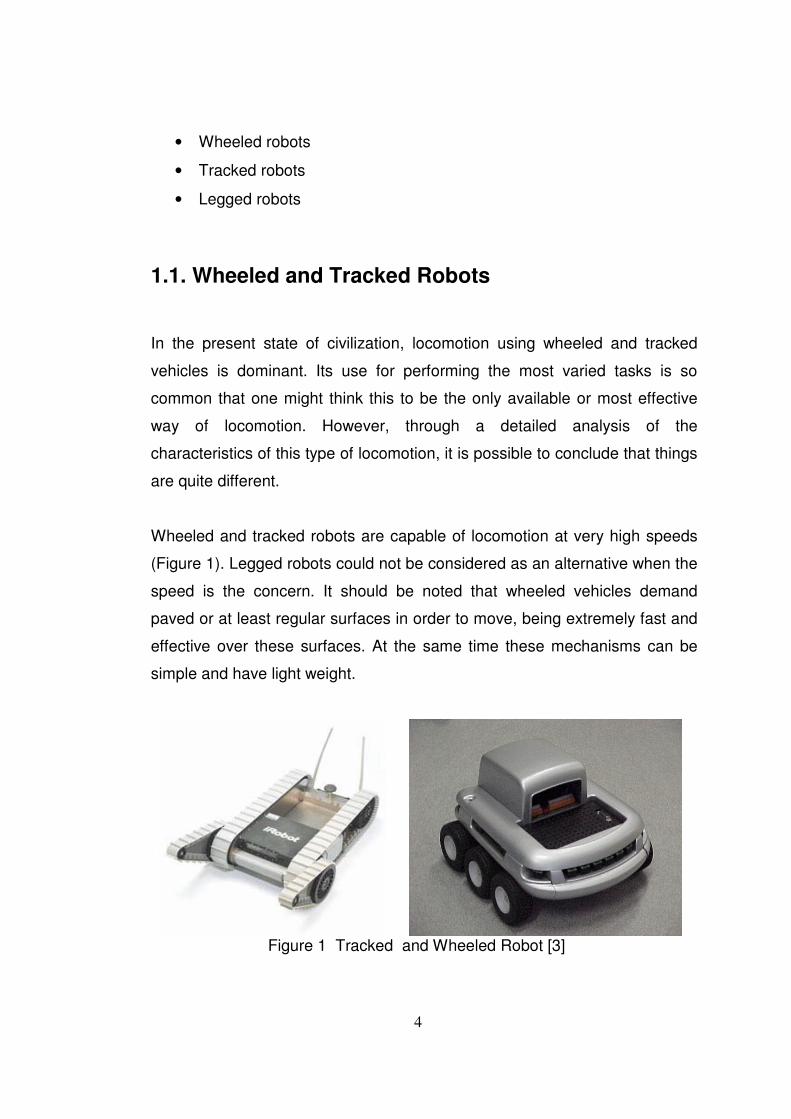
Figure 1 Tracked and Wheeled Robot [3] ........................................................... 4
Figure 2 Raibert’s Pogostick ................................................................................. 11
Figure 3 ARL Monopod II Experiment Setup ..................................................... 12
Figure 4 WABOT-1 ................................................................................................. 13
Figure 5 WABOT-2 ................................................................................................. 14
Figure 6 ASIMO (Advanced Step in Innovative MObility) ................................ 16
Figure 7 First Quadruped Machine ...................................................................... 17
Figure 8 General Electric Quadruped ................................................................. 18
Figure 9 Phoney Poney ......................................................................................... 18
Figure 10 Scout I .................................................................................................... 19
Figure 11 OSU Hexapod ....................................................................................... 20
Figure 12 Boadicea ................................................................................................ 21
Figure 13 TUM Robot ............................................................................................ 21
Figure 14 Whegs I .................................................................................................. 21
Figure 15 Rhex - Compliant-Legged Hexapod Robot ...................................... 22
Figure 16 ADAMS Model ...................................................................................... 24
Figure 17 Experimental Setup .............................................................................. 24
Figure 18 Optimization of Crank Driver Mechanism Part ............................... 26
Figure 19 Durability Analysis of Spare-wheel Carrier ....................................... 26
Figure 20 The base and crash frame assembly ................................................ 29
Figure 21 The photograph of the main body of Rhex (base and crash frame) with motor and gearbox assemblies. .................................................................... 29
Figure 22 The crash frame of RHex .................................................................... 30
Figure 23 The new motor mounting part. ........................................................... 31
Figure 24 The base frame ..................................................................................... 32
Figure 25 Frame Left Rail ..................................................................................... 33
Figure 26 Frame end angle .................................................................................. 33
Figure 27 Frame middle angle ............................................................................. 33
Figure 28 Frame assembly ................................................................................... 34
Figure 29 Hip bearing seat and Hip bearing spacer ......................................... 35
Figure 30 Exploded view of the motor mounting assembly ............................. 35
Figure 31 Leg mounted to the motor mounting assembly ............................... 36
Figure 32 The orientation of the multilayer fiberglass ....................................... 37
Figure 33 Motor driver board holder .................................................................... 38
Figure 34 The final assembly of the robot .......................................................... 38
Figure 35 Side support .......................................................................................... 39
Figure 36 Side supports and PC104 housing assembly .................................. 39
Figure 37 Final assembly of the manufactured parts ........................................ 40
Figure 38 Box model .............................................................................................. 44
Figure 39 CAD import from Patran ...................................................................... 44
x
Figure 40 Import menu in ADAMS software ...................................................... 45
Figure 41 Import Menu in MSC PATRAN ........................................................... 46
Figure 42 Mesh properties definition ................................................................... 47
Figure 43 Tetrahedron element meshing with 1899 elements ......................... 48
Figure 44 Tetrahedron element meshing with 35811 elements....................... 48
Figure 45 Create Node – The connection point ................................................ 49
Figure 46 Node definition and connection .......................................................... 50
Figure 47 Material creation and property definition .......................................... 51
Figure 48 Material assigning ................................................................................ 51
Figure 49 Analysis settings-1 ............................................................................... 52
Figure 50 Analysis settings -2 .............................................................................. 53
Figure 51 Analysis settings-3 ............................................................................... 54
Figure 52 Function Builder Menu ......................................................................... 55
Figure 53 Defined motions of the legs ................................................................ 56
Figure 54 Simple Pendulum Model ..................................................................... 58
Figure 55 Assigning variables .............................................................................. 58
Figure 56 Torque variable ..................................................................................... 59
Figure 57 Position variable ................................................................................... 59
Figure 58 Assigning torque variable to the applied torque .............................. 60
Figure 59 Defining control plant ........................................................................... 61
Figure 60 The final state of the control plant submenu .................................... 61
Figure 61 “Adams_sub” block, represents the simple pendulum system ..... 62
Figure 62 Closed loop control of the angular position ...................................... 63
Figure 63 Torque input to the legs ....................................................................... 65
Figure 64 Definition of the inputs and outputs as a variable ........................... 65
Figure 65 Torque variable assignment ............................................................... 66
Figure 66 Angular Position of the Legs ............................................................... 66
Figure 67 Control Plant Definition ........................................................................ 67
Figure 68 Final view of the Control Plant build menu ....................................... 68
Figure 69 Calling m-file from MATLAB ............................................................... 68
Figure 70 A closed loop PID controller ............................................................... 69
Figure 71 Reference position presentation [44] ................................................ 70
Figure 72 Forward body velocity for a simulation run with tc = 0.5s,.............. 72
Figure 73 Left and right tripod angular velocity profile ..................................... 73
Figure 74 Angular position of left and right tripod ............................................. 73
Figure 75 Position and Velocity of the body in X direction .............................. 74
Figure 76 Body fluctuation in y direction ............................................................. 75
Figure 77 Torque graph of one leg ...................................................................... 76
Figure 78 Torque-speed curve of RE30 motor [48] .......................................... 76
Figure 79 Velocity in x direction versus body fluctuation in y direction ......... 77
Figure 80 Final ADAMS Sub Block ..................................................................... 78
Figure 81 Reference angle input and real angular position of the leg in the same graph ............................................................................................................... 80
Figure 82 The difference between reference and real angular position of the left tripod ................................................................................................................... 80
Figure 83 The difference between reference and real angular position of the right tripod ................................................................................................................. 81
xi
Figure 84 Angular velocity profile of left and right tripods ................................ 83
Figure 85 Angular position profile of left and right tripod ................................. 83
Figure 86 Position and velocity of the body in x direction ................................ 84
Figure 87 Body fluctuation in y direction ............................................................. 85
Figure 88 Velocity in x direction versus body fluctuation in y direction ......... 85
Figure 89 “Φ” angle of the body orientation ....................................................... 86
Figure 90 “θ” angle of the body orientation ........................................................ 87
Figure 91 Torque requirement of the left rear leg ............................................. 87
Figure 92 Angular velocity input of the left and right tripods ........................... 88
Figure 93 Position and velocity in x direction ..................................................... 89
Figure 94 Body fluctuation in y direction ............................................................. 89
Figure 95 Velocity in x direction versus body fluctuation in y direction ......... 90
Figure 96 “θ” angle of the body versus velocity in x direction ......................... 91
Figure 97 “Φ” angle of the body versus velocity in x direction ........................ 91
Figure 98 Torque requirement of one leg ........................................................... 92
Figure 99 Position and velocity in x direction of RHex with elastic modulus of leg 10 GPa ................................................................................................................ 93
Figure 100 Body Fluctuation in “y” direction ...................................................... 94
Figure 101 Torque requirement of one leg for elastic modulus of 10 GPa ... 95
Figure 102 The velocity profile comparison of the three simulation results .. 95
Figure 103 The position of the body in x direction ............................................ 96
Figure 104 The velocity of RHex in x direction .................................................. 97
Figure 105 Body fluctuation in y direction .......................................................... 98
Figure 106 “Φ” angle of the body versus velocity in x direction ...................... 98
Figure 107 “θ” angle of the body versus velocity in x direction ....................... 99
Figure 108 Position of RHex in x direction ......................................................... 99
Figure 109 The velocity of RHex in x direction ................................................ 100
Figure 110 The body fluctuation in y direction ................................................. 100
Figure 111 “Φ” angle of the body versus velocity in x direction .................... 101
Figure 112 “θ” angle of the body versus velocity in x direction ..................... 101
Figure 113 The position of RHex in x direction ............................................... 102
Figure 114 The velocity of RHex in x direction ................................................ 103
Figure 115 The body fluctuation in y direction ................................................. 103
Figure 116 “Φ” angle of the body versus velocity in x direction .................... 104
Figure 117 “θ” angle of the body versus velocity in x direction ..................... 104
Figure 118 The comparison of the displacement in x direction .................... 105
Figure 119 The comparison of the velocity in x direction ............................... 106
Figure 120 The comparison of the body fluctuation in y direction ................ 106
Figure 121 Angular velocities of left and right tripods .................................... 107
Figure 122 Position and velocity in x direction ................................................ 108
Figure 123 Body fluctuation in y direction ........................................................ 109
Figure 124 “Φ” angle of the body versus velocity in x direction .................... 109
Figure 125 “θ” angle of the body versus velocity in x direction ..................... 110
Figure 126 Screenshot of the start of the slow phase .................................... 110
1
CHAPTER 1
INTRODUCTION Robots are wide range of devices with different levels of autonomy,
intelligence, and mobility. They acquire sensory data, process the
information, actuate motion and react to the external environment in a
predictable and controllable manner. Robots with a high level of intelligence
are capable of performing complex tasks autonomously. Their control
architectures require more sophisticated design and implementation than
those of robots with a low level of intelligence.
The complexity of robots shows differences according to the time that they
have been invented. Mankind has long ago tried to build machines that
looked like living beings or even resembled human beings. The beginning of
robots may be traced to the Greek Engineer Ctesibius (c. 270 BC) who
applied his knowledge of pneumatics and hydraulics to produce the first
organ and water clocks with moving figures. Philo of Byzantium (c. 200 BC),
one of the Ctesibius students, wrote “Mechanical Collection” describing his
teacher’s work. Later, based on that book, Hero of Alexandria (c. AD 85)
wrote “On Automatic Theaters, On Pneumatics and On Mechanics”,
presenting the first well documented workable robots outside of mythology.
The Greeks entertainment robots were designed for limited and repetitive
jobs and didn’t have to perform more demanding functions. The Greeks had
a specific word to name these machines: “automatos”. The current word
automation is derived from this word and means “machine that imitates the
figure and movements of an animate being” [1].
2
In the early ninth century the Khalif of Baghdad (786–833) assigned three
men, to acquire all Greek texts that had been preserved by monasteries and
scholars during the decline and fall of western civilization. They produced the
large book Kitab al-Hiyal (The Book of Ingenious Devices) based on the
works they collected. Over a hundred devices were described in that book.
The next significant automation work was compiled by a Turkman, Badi’as-
Zaman Isma’il bin Ar-Razzaz Al-Jazari (1150–1220), He gave detailed
descriptions to the science of ingenious mechanisms and compilation or
variation of existing designs besides . Al-Jazari may have constructed many
of the mechanisms also.. Thus, the greatest contribution the Arabs made,
besides preserving, disseminating and building on the work of the Greeks,
was the concept of practical application. This was the key element that was
missing in Greek robotic science [2].
The Renaissance revived not only the interest in Greek art and science, but
also created a desire to compete with the ancients achievements. Inspired by
this, Leonardo da Vinci (1452–1519) was actively engaged in verifying Greek
reconstructions, an activity that no doubt inspired him to devise water
powered organs and clocks equipped with Jacque mart, or Jack figures, for
striking the hours.
In the 18th century mechanical puppets were first built in Europe. An
established clock and watch making industry in Switzerland made available
the skilled craftsmen and base technology needed to build those machines.
The Scribe, the Draftsman and the Musician display a high degree of
anthropomorphism for their time. Basically entertainment devices, the three
figures were programmable through stacked cams, presenting sophisticated
movements. Making their public debut in 1774, they were the work of Pierre
Jaquet-Droz (1721-1790) and his assistants, chiefly Jean Frederic Leschat.
The pioneer Jaquet-Droz created lasting examples of the craftsman’s art. An
early innovation was a tiny mechanical singing bird fitted into a snuffbox [2].
In 1801 Joseph Maria Jacquard introduced the next significant innovation
3
and invented the automatic draw loom. The draw loom would punch cards
and was used to control the lifting of thread in fabric factories. This was the
first invention to be able to store a program and control a machine.
Ever since, developments have mainly been driven to resemble physical
aspects, although in the last few years, one of the main challenges in
robotics has been to enrich these machines with a grade of intelligence in
order to allow them to extract information from the environment and use that
knowledge to carry out their tasks safely. Although it is not clear which of the
previously mentioned devices should be considered the first robot, it is clear
the origin of the term robot. This word was introduced in a play called R.U.R.
(Rossum’s Universal Robots), by a Czechoslovakian playwright named Karel
Capek. R.U.R. was a play about human-like servants that were artificially
created out of biological tissues to serve humans in factories and in the army.
Capek called these artificial workers “robots”, from the Czech word “robota”,
meaning slave work.
The robot evolution depends on the evolution on hardware. It has contributed
to create robots with sensors and actuators which allow the imitation of the
human beings and the animal’s way of displacement. Concerning the
software evolution, it has allowed supplying robots with intelligence and with
the capability of learning and of mimicking the reasoning capacity and
emotions of humans.
Today’s robotic systems may be classified, generically, into two major areas:
• manipulation robotics
• mobile robotics.
Mobile robots have the capability to move around in their environment and
are not fixed to one physical location. They could be classified according to
the way that they use to move.
4
• Wheeled robots
• Tracked robots
• Legged robots
1.1. Wheeled and Tracked Robots
In the present state of civilization, locomotion using wheeled and tracked
vehicles is dominant. Its use for performing the most varied tasks is so
common that one might think this to be the only available or most effective
way of locomotion. However, through a detailed analysis of the
characteristics of this type of locomotion, it is possible to conclude that things
are quite different.
Wheeled and tracked robots are capable of locomotion at very high speeds
(Figure 1). Legged robots could not be considered as an alternative when the
speed is the concern. It should be noted that wheeled vehicles demand
paved or at least regular surfaces in order to move, being extremely fast and
effective over these surfaces. At the same time these mechanisms can be
simple and have light weight.
Figure 1 Tracked and Wheeled Robot [3]
5
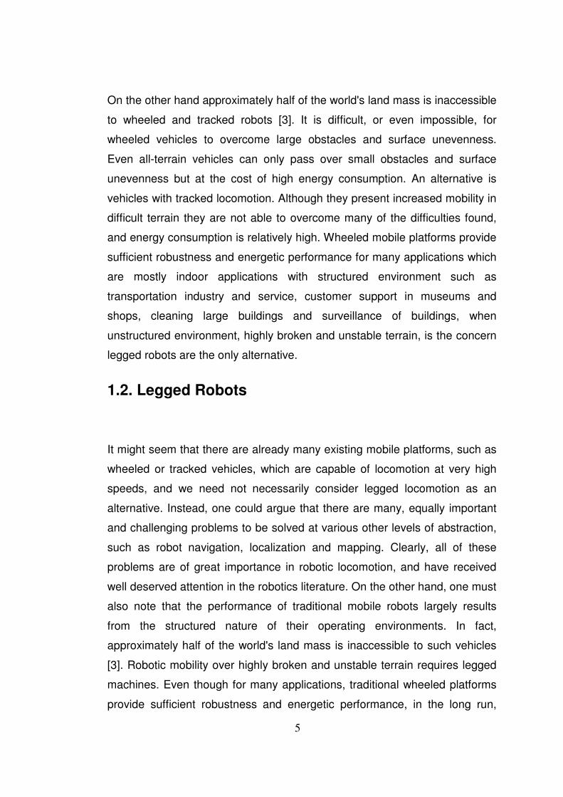
On the other hand approximately half of the world's land mass is inaccessible
to wheeled and tracked robots [3]. It is difficult, or even impossible, for
wheeled vehicles to overcome large obstacles and surface unevenness.
Even all-terrain vehicles can only pass over small obstacles and surface
unevenness but at the cost of high energy consumption. An alternative is
vehicles with tracked locomotion. Although they present increased mobility in
difficult terrain they are not able to overcome many of the difficulties found,
and energy consumption is relatively high. Wheeled mobile platforms provide
sufficient robustness and energetic performance for many applications which
are mostly indoor applications with structured environment such as
transportation industry and service, customer support in museums and
shops, cleaning large buildings and surveillance of buildings, when
unstructured environment, highly broken and unstable terrain, is the concern
legged robots are the only alternative.
1.2. Legged Robots
It might seem that there are already many existing mobile platforms, such as
wheeled or tracked vehicles, which are capable of locomotion at very high
speeds, and we need not necessarily consider legged locomotion as an
alternative. Instead, one could argue that there are many, equally important
and challenging problems to be solved at various other levels of abstraction,
such as robot navigation, localization and mapping. Clearly, all of these
problems are of great importance in robotic locomotion, and have received
well deserved attention in the robotics literature. On the other hand, one must
also note that the performance of traditional mobile robots largely results
from the structured nature of their operating environments. In fact,
approximately half of the world's land mass is inaccessible to such vehicles
[3]. Robotic mobility over highly broken and unstable terrain requires legged
machines. Even though for many applications, traditional wheeled platforms
provide sufficient robustness and energetic performance, in the long run,
6
systems capable of operating in the widest variety of terrain conditions, will
be legged robots. Nonetheless, legged platforms present many difficulties
from an engineering point of view. Unlike traditional mobile robots, the control
of these platforms requires a complete understanding of their dynamics. Most
of their behavioral and energetic performance relies on the inherent
properties of their mechanical structure, for which we currently have very few
well developed analytical tools. The coordination of the large number of joints
and the redundancy in the actuated degrees of freedom compared to the
small number of task degrees of freedom, present novel challenges in the
design of controllers for such systems. [4]
Legged locomotion vehicles present superior mobility in natural terrains,
since these vehicles may use discrete footholds for each foot, in contrast to
wheeled vehicles, which need a continuous support surface. Therefore,
legged vehicles may move over irregular terrain, by varying their legs
configuration in order to adapt themselves to surface irregularities. In
addition, feet may establish contact with the ground at selected points in
accordance with the terrain conditions. For these reasons, legs are inherently
adequate systems for locomotion over irregular ground. When the vehicles
move over soft surfaces, i.e. sandy soil, the ability to use discrete footholds in
the ground can also improve the energy consumption, since they deform the
terrain less than wheeled or tracked vehicles and, therefore, the energy
needed to get out of depressions is lower [5]. Besides, the contact area
between the foot and the ground can be made in such a way that the ground
support pressure can be low. Moreover, the use of multiple degrees of
freedom in the leg joints, allows legged vehicles to change their heading
without slippage. It is also possible to vary the body height, introducing a
damping and decoupling effect between terrain irregularities and the vehicle
body. This is particularly true in the case that they move, for instance, over
the outside surface of pipes, in order to increase their balance ability [6].

7
Another advantage that has recently been investigated, concerns failure
tolerance during static stable locomotion. The consequence of a failure in
one of the wheels of a wheeled vehicle is a severe loss of mobility, since all
wheels on these kinds of vehicles should be in permanent contact with the
ground during locomotion. However, legged vehicles may contain redundant
legs and, therefore, can maintain static balance and continue locomotion
even with one or more legs damaged [7], [8], [9], [10], [11].
Finally, it should be mentioned that legs can be used not only for locomotion,
but also for other purposes. For instance, the body can be actively actuated
while feet are fixed to the ground, working as an active support base to help
the motion of a manipulator [12] or a tool [13] mounted on the body. As an
alternative to the assembly of a manipulator on a robot body, multi-legged
robots can use one or more of its legs to manipulate objects, as is possible
with some animals (several animals use their legs to hold, manipulate and
transport objects). As an example, Takita et al. (2003) [14] present a biped
robot, whose structure is inspired by dinosaurs, on which the tail is used to
help maintain balance during locomotion and during manipulation tasks that
the robot performs with its neck. The tail is also used so that the robot can
stand on it, making a stable support tripod. Hirose and Kato (1998) [15]
propose using the TITAN-VIII quadruped robot in the task of landmine
detection and removal. For this purpose it uses one of the robot legs as a
manipulator arm, with the possibility of being equipped with a set of different
end effectors.
Omata et al. (2002) [16] also propose the adoption of a quadruped robot for
manipulation tasks, in which two of its legs are used for locomotion, while the
body and remaining legs are used for object manipulation. Takahashi et al.
(2000) [17] and Koyachi et al. (2002) [18] present similar solutions to the
previous ones, but for hexapod robots. The solutions described have as
advantages reduction in system weight and a corresponding increase in

8
energetic autonomy, because otherwise it would be necessary to mount arms
on the locomotion system, these devoted only to manipulations tasks.
So far the structure, area of use and properties of the wheeled, tracked and
legged robots are mentioned. To summarize, the majority of mobile robots
are wheeled robots which are easier to design, construct, and control than
legged robots. Wheeled robots are suitable for traversing level terrain. They
need specially designed mechanisms for moving in outdoor environments. In
general, legged robots have more complexity in design and control, but they
are more practical in some applications than wheeled robots. Legged robots
have their advantages and disadvantages compared with wheeled robots.
Legged robots have many advantages over wheeled robots. In order to move
effectively, a wheeled robot must have all wheels contacting the surface all
the time, while a legged robot can travel by using some legs touching the
ground at any given time. As a result, legged robots are more suitable for
traversing on non-continuous surfaces especially the natural terrain and
outdoor environments. In addition, they can step over small obstacles. Also
they can walk up and down stairs or slopes. With well-designed leg
mechanisms, they can step or even jump over wide abysses. They can travel
over irregular terrain while maintaining smooth motion of their center of
gravity by varying the vertical stride of each leg. Legged robots can also
move on soft ground, such as sand, mud, and loose surfaces, where
wheeled robots might slip. Legged robots disturb and do damage to the
ground less than wheel robots. Furthermore, legged robots can maneuver
around using a smaller area than wheeled robots. They can change direction
by changing their foot placement. The average speed of legged robots is the
same for all types of terrain, while the speed of wheeled robots decreases
when they are moving on irregular surfaces. These advantages make legged
robots appealing for natural terrain exploration. On the other hand, legged
robots have some disadvantages as compared to wheeled robots. Legged
robots have more mechanical complexity than wheeled robots because each
leg has many links and joints. Consequently, complex electronic systems for
9
controlling and powering those joints are required as well as sensor systems
for determining the status of each leg. Typically, the more complex the
system is, the more expensive the total cost of the system is. Furthermore,
the control algorithms for legged robots are more complex than wheeled
robots. The movement of all joints must be synchronized and respond to
sensory input from all legs. In addition, on level terrain, legged robots can not
achieve the speed of wheeled robots [23]. Although legged robots have some
disadvantages and may not be suitable for some applications, there are
many advantages of them. Legged robots are by nature strongly non-linear,
high-dimensional systems whose full complexity permits neither tractable
mathematical analysis nor comprehensive numerical study [19].
1.3. Present Day Legged Robots
Today’s legged locomotion vehicles are classified according to the number of
the legs.
• Monopod
• Biped
• Quadruped
• Hexapod
• Multi-legged
1.3.1. Monopod Robots
In the case of one legged robots, locomotion is performed through hops.
Therefore, these machines are also known as hopping robots. Although the
most approximate natural example of hopping locomotion is the kangaroo,
this model can also be applied to running bipeds, which alternate between
one or no foot in contact with the ground. These machines keep an active
balance as they move, achieving dynamic stability, allowing a better
10
understanding of the energy exchanges that occur during a locomotion cycle,
and emphasizing the active and dynamic stability problems, without requiring
leg coordination schemes.
Matsuoka was the first to build a machine according to these concepts, which
means, with ballistic flight periods in which the feet lose contact with the
ground. His objective was to model the cyclic jumps in human locomotion. In
order to achieve this objective, Matsuoka formulated a model, consisting of a
body and a weightless leg (to simplify the problem), and considered that the
support phase duration was short when compared with the ballistic flight
phase. This motion, in which almost the entire cycle is spent on the transfer
phase, minimizes the inclination influence during the support phase [20].
To test the control system, Matsuoka built a planar one legged hopping
machine. The machine stands over an inclined table (10° with the horizontal),
rolling on ball bearings. An electrical solenoid gave a fast impulse to the foot,
in such a way that the support period was small. The machine hopped in
place with a period of 1 hop s-1 and could walk forward and backward over
the table.
Raibert was another researcher working on dynamical locomotion systems
and, in 1983, built at Carnegie Mellon University (CMU) a hopping robot. This
system, formed by a body and a single leg, needed to hop continuously in
order to maintain balance [21]. The body constituted the main structure,
which transported the needed actuators and instrumentation for the machine
operation. The leg could be extended, varying its width, and was equipped
with springs along its axis. Several sensors measured the body inclination
angle, the hip angle, the leg width, the spring leg stiffness and the ground
contact. This first machine was limited to operate on a level surface and,
therefore, could only move up and down, front and back, or rotate in the
plane. A second hopping machine, named Pogostick (Figure 2), had an
additional hip joint to allow the leg to move sideways, as well as forward and
back.
11
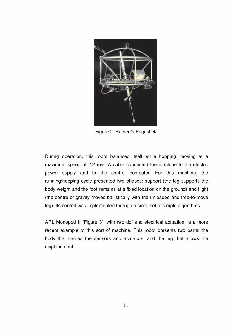
Figure 2 Raibert’s Pogostick
During operation, this robot balanced itself while hopping; moving at a
maximum speed of 2.2 m/s. A cable connected the machine to the electric
power supply and to the control computer. For this machine, the
running/hopping cycle presented two phases: support (the leg supports the
body weight and the foot remains at a fixed location on the ground) and flight
(the centre of gravity moves ballistically with the unloaded and free-to-move
leg). Its control was implemented through a small set of simple algorithms.
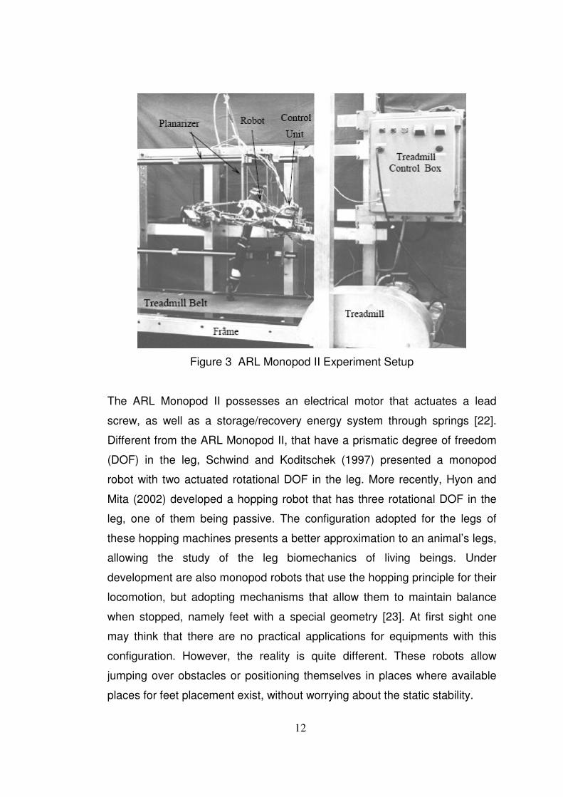
ARL Monopod II (Figure 3), with two dof and electrical actuation, is a more
recent example of this sort of machine. This robot presents two parts: the
body that carries the sensors and actuators, and the leg that allows the
displacement.
12
Figure 3 ARL Monopod II Experiment Setup
The ARL Monopod II possesses an electrical motor that actuates a lead
screw, as well as a storage/recovery energy system through springs [22].
Different from the ARL Monopod II, that have a prismatic degree of freedom
(DOF) in the leg, Schwind and Koditschek (1997) presented a monopod
robot with two actuated rotational DOF in the leg. More recently, Hyon and
Mita (2002) developed a hopping robot that has three rotational DOF in the
leg, one of them being passive. The configuration adopted for the legs of
these hopping machines presents a better approximation to an animal’s legs,
allowing the study of the leg biomechanics of living beings. Under
development are also monopod robots that use the hopping principle for their
locomotion, but adopting mechanisms that allow them to maintain balance
when stopped, namely feet with a special geometry [23]. At first sight one
may think that there are no practical applications for equipments with this
configuration. However, the reality is quite different. These robots allow
jumping over obstacles or positioning themselves in places where available
places for feet placement exist, without worrying about the static stability.
13
1.3.2. Biped Robots Bipeds, or two-legged robots, are mostly biologically inspired by human
anatomy. Many research groups have developed humanoid robots but biped
locomotion has complexity in balance and stability control so the research on
biped locomotion, when compared with the multi-legged case, has advanced
more slowly. Their movement requires considerable sensor information and
dynamic control of the center of gravity motion.
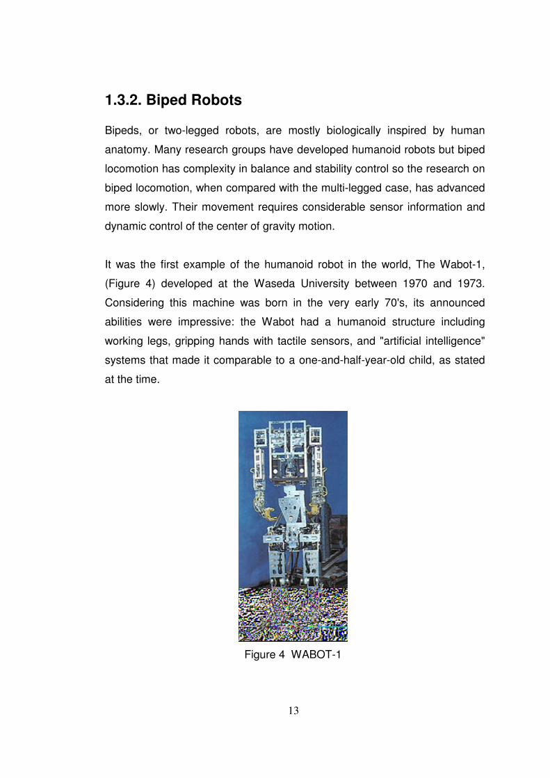
It was the first example of the humanoid robot in the world, The Wabot-1,
(Figure 4) developed at the Waseda University between 1970 and 1973.
Considering this machine was born in the very early 70's, its announced
abilities were impressive: the Wabot had a humanoid structure including
working legs, gripping hands with tactile sensors, and "artificial intelligence"
systems that made it comparable to a one-and-half-year-old child, as stated
at the time.
Figure 4 WABOT-1
14
Wabot-1 is able to achieve "static walking", that is, transferring its center of
gravity from one leg to another and moving the leg/raising the feet
accordingly. AI interaction systems included a communication system
(speech synthesis, speech recognition) and a visual system. It was able to
"communicate" in Japanese. The development that led to the Wabot-1
actually began in 1967 with the WL-1 "biped robot" project. The experiments
at the Waseda University first focused on the developments of robotic legs.
The WL-5 was used as the Wabot-1 lower limb, and development of the WL
series lasted long after the Wabot-1 was introduced.
In 1984, Waseda University presented the Wabot-2 (Figure 5). This machine
was the first attempt of specializing a robot for domestic use. The chosen
activity was music, and the Wabot-2 got worldwide famous as the first robot
in the world which played piano. Playing a keyboard instrument was set up
as an intelligent task that the WABOT-2 aimed to accomplish, since an
artistic activity such as playing a keyboard instrument would require human-
like intelligence and ability. Therefore the WABOT-2 was defined as a
"specialist robot" rather than a versatile robot like the WABOT-1.
Figure 5 WABOT-2
15
The robot musician WABOT-2 can talk with a person, read a normal musical
score with his eye and play tunes of average difficulty on an electronic organ.
The WABOT-2 is also able of accompanying a person while he listens to the
person singing. The WABOT-2 was the first milestone in developing a
"personal robot”. The development of new robots researches continues at the
Waseda University. Since 1985, new robots from the Waseda University are
presented under the "Wabian" name.
Nowadays there is a large variety of biped robots presenting humanoid
shape and having good locomotion capabilities.
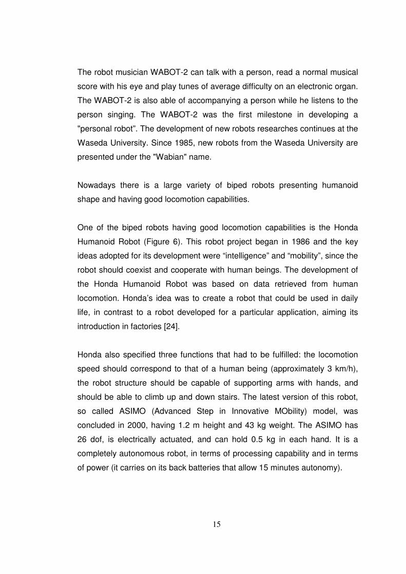
One of the biped robots having good locomotion capabilities is the Honda
Humanoid Robot (Figure 6). This robot project began in 1986 and the key
ideas adopted for its development were “intelligence” and “mobility”, since the
robot should coexist and cooperate with human beings. The development of
the Honda Humanoid Robot was based on data retrieved from human
locomotion. Honda’s idea was to create a robot that could be used in daily
life, in contrast to a robot developed for a particular application, aiming its
introduction in factories [24].
Honda also specified three functions that had to be fulfilled: the locomotion
speed should correspond to that of a human being (approximately 3 km/h),
the robot structure should be capable of supporting arms with hands, and
should be able to climb up and down stairs. The latest version of this robot,
so called ASIMO (Advanced Step in Innovative MObility) model, was
concluded in 2000, having 1.2 m height and 43 kg weight. The ASIMO has
26 dof, is electrically actuated, and can hold 0.5 kg in each hand. It is a
completely autonomous robot, in terms of processing capability and in terms
of power (it carries on its back batteries that allow 15 minutes autonomy).
16
Figure 6 ASIMO (Advanced Step in Innovative MObility)
Sakagami present an evolved version of the ASIMO model, prepared to
perform people attendance tasks and museum visit guiding, due to the
integration of a vision and audition sensors set and a human gesture
recognition system, allowing this humanoid to interact with human beings.
[25]
1.3.3. Quadruped Robots
Quadrupeds, or four-legged robots, are similar to some reptiles and
mammals [26]. Reptiles evolved their leg arrangement to be wide and stable
which is appropriate to their environment. The disadvantages of reptilian
motions are the twisting movement of the bodyline, and the hip has to
support the body weight. Dissimilar to reptiles, the mammalian leg
arrangement has no disadvantages except difficulty in stability control [27].
17
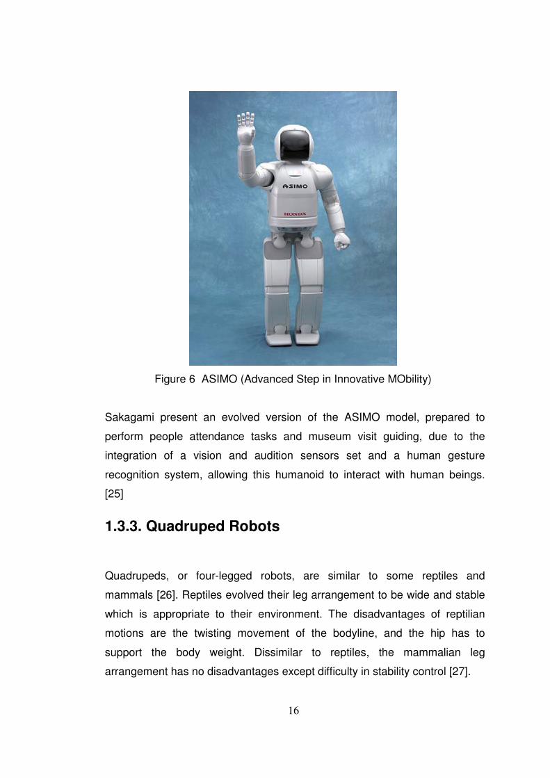
Figure 7 First Quadruped Machine
Figure 7 shows a drawing of the first quadruped machine, named The
Mechanical Horse, proposed by L. A. Rygg. This machine was patented on
14 February 1893, but there is no evidence to prove that he actually built this
machine [28]
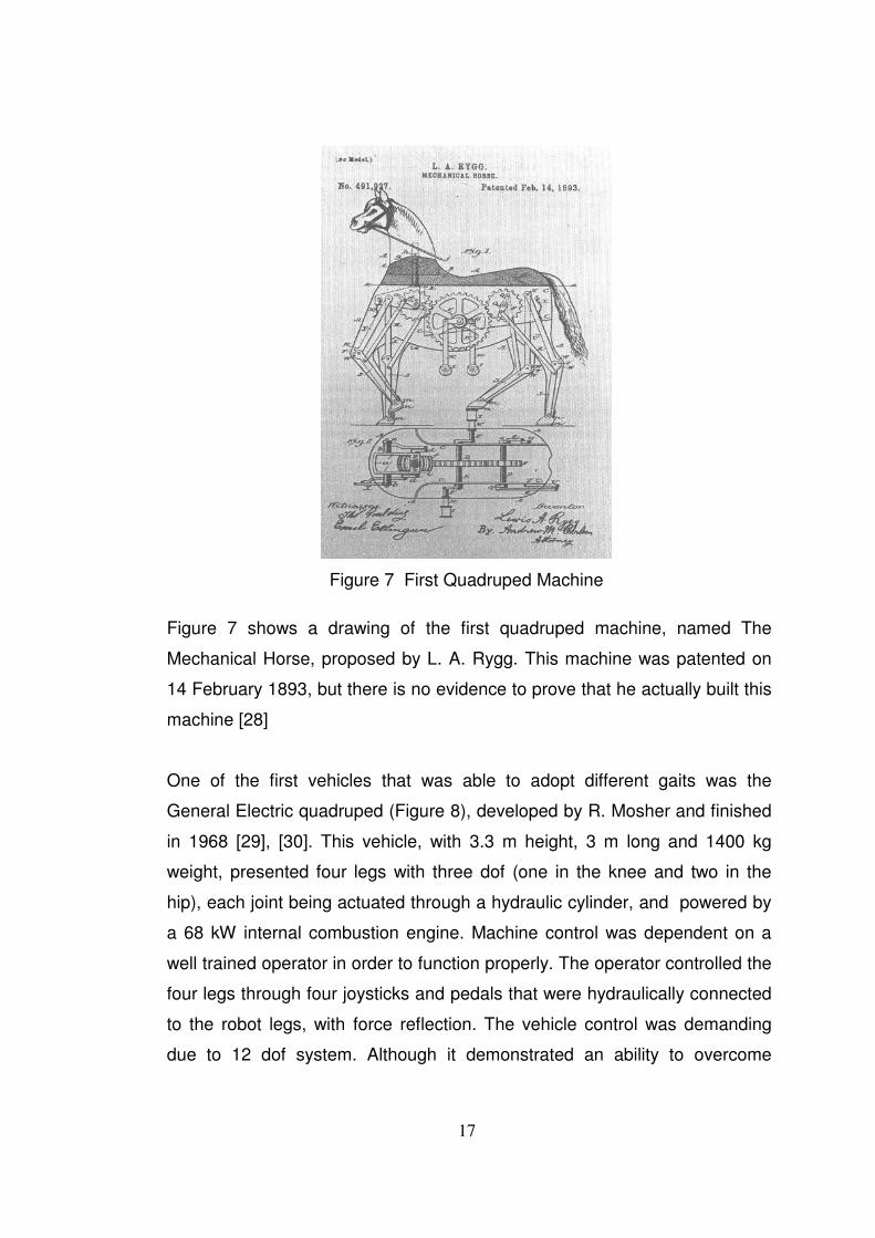
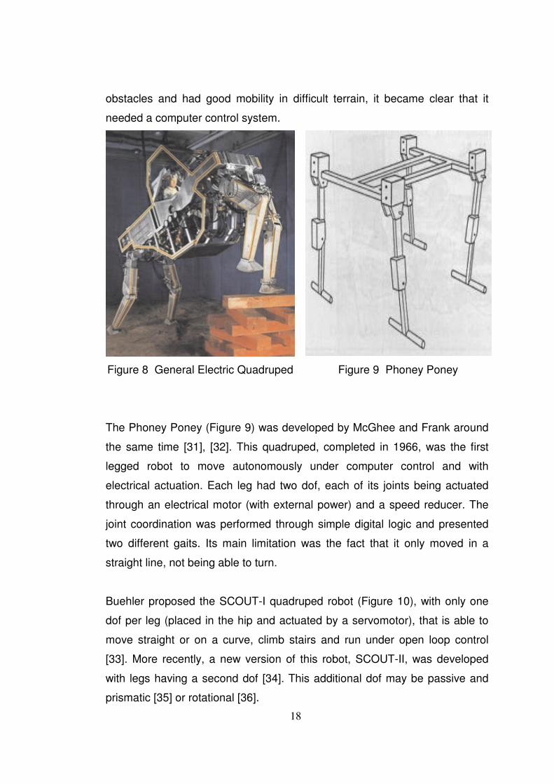
One of the first vehicles that was able to adopt different gaits was the
General Electric quadruped (Figure 8), developed by R. Mosher and finished
in 1968 [29], [30]. This vehicle, with 3.3 m height, 3 m long and 1400 kg
weight, presented four legs with three dof (one in the knee and two in the
hip), each joint being actuated through a hydraulic cylinder, and powered by
a 68 kW internal combustion engine. Machine control was dependent on a
well trained operator in order to function properly. The operator controlled the
four legs through four joysticks and pedals that were hydraulically connected
to the robot legs, with force reflection. The vehicle control was demanding
due to 12 dof system. Although it demonstrated an ability to overcome
18
obstacles and had good mobility in difficult terrain, it became clear that it
needed a computer control system.
Figure 8 General Electric Quadruped Figure 9 Phoney Poney
The Phoney Poney (Figure 9) was developed by McGhee and Frank around
the same time [31], [32]. This quadruped, completed in 1966, was the first
legged robot to move autonomously under computer control and with
electrical actuation. Each leg had two dof, each of its joints being actuated
through an electrical motor (with external power) and a speed reducer. The
joint coordination was performed through simple digital logic and presented
two different gaits. Its main limitation was the fact that it only moved in a
straight line, not being able to turn.
Buehler proposed the SCOUT-I quadruped robot (Figure 10), with only one
dof per leg (placed in the hip and actuated by a servomotor), that is able to
move straight or on a curve, climb stairs and run under open loop control
[33]. More recently, a new version of this robot, SCOUT-II, was developed
with legs having a second dof [34]. This additional dof may be passive and
prismatic [35] or rotational [36].
19
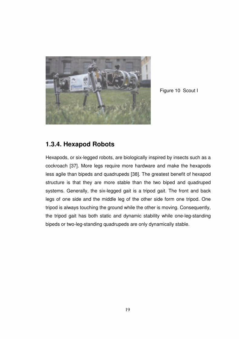
Figure 10 Scout I
1.3.4. Hexapod Robots Hexapods, or six-legged robots, are biologically inspired by insects such as a
cockroach [37]. More legs require more hardware and make the hexapods
less agile than bipeds and quadrupeds [38]. The greatest benefit of hexapod
structure is that they are more stable than the two biped and quadruped
systems. Generally, the six-legged gait is a tripod gait. The front and back
legs of one side and the middle leg of the other side form one tripod. One
tripod is always touching the ground while the other is moving. Consequently,
the tripod gait has both static and dynamic stability while one-leg-standing
bipeds or two-leg-standing quadrupeds are only dynamically stable.
20
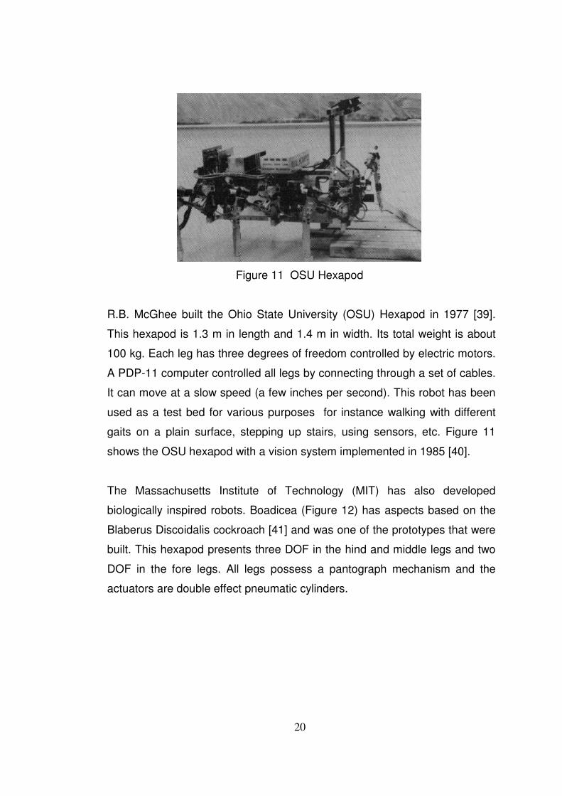
Figure 11 OSU Hexapod
R.B. McGhee built the Ohio State University (OSU) Hexapod in 1977 [39].
This hexapod is 1.3 m in length and 1.4 m in width. Its total weight is about
100 kg. Each leg has three degrees of freedom controlled by electric motors.
A PDP-11 computer controlled all legs by connecting through a set of cables.
It can move at a slow speed (a few inches per second). This robot has been
used as a test bed for various purposes for instance walking with different
gaits on a plain surface, stepping up stairs, using sensors, etc. Figure 11
shows the OSU hexapod with a vision system implemented in 1985 [40].
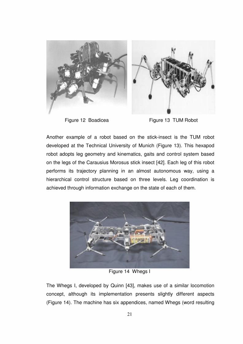
The Massachusetts Institute of Technology (MIT) has also developed
biologically inspired robots. Boadicea (Figure 12) has aspects based on the
Blaberus Discoidalis cockroach [41] and was one of the prototypes that were
built. This hexapod presents three DOF in the hind and middle legs and two
DOF in the fore legs. All legs possess a pantograph mechanism and the
actuators are double effect pneumatic cylinders.
21
Figure 12 Boadicea Figure 13 TUM Robot
Another example of a robot based on the stick-insect is the TUM robot
developed at the Technical University of Munich (Figure 13). This hexapod
robot adopts leg geometry and kinematics, gaits and control system based
on the legs of the Carausius Morosus stick insect [42]. Each leg of this robot
performs its trajectory planning in an almost autonomous way, using a
hierarchical control structure based on three levels. Leg coordination is
achieved through information exchange on the state of each of them.
Figure 14 Whegs I
The Whegs I, developed by Quinn [43], makes use of a similar locomotion
concept, although its implementation presents slightly different aspects
(Figure 14). The machine has six appendices, named Whegs (word resulting
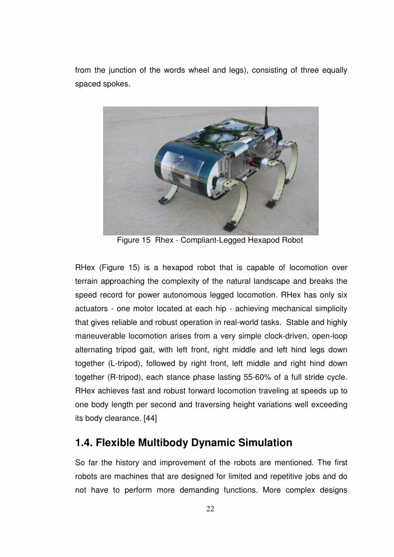
22
from the junction of the words wheel and legs), consisting of three equally
spaced spokes.
Figure 15 Rhex - Compliant-Legged Hexapod Robot
RHex (Figure 15) is a hexapod robot that is capable of locomotion over
terrain approaching the complexity of the natural landscape and breaks the
speed record for power autonomous legged locomotion. RHex has only six
actuators - one motor located at each hip - achieving mechanical simplicity
that gives reliable and robust operation in real-world tasks. Stable and highly
maneuverable locomotion arises from a very simple clock-driven, open-loop
alternating tripod gait, with left front, right middle and left hind legs down
together (L-tripod), followed by right front, left middle and right hind down
together (R-tripod), each stance phase lasting 55-60% of a full stride cycle.
RHex achieves fast and robust forward locomotion traveling at speeds up to
one body length per second and traversing height variations well exceeding
its body clearance. [44]
1.4. Flexible Multibody Dynamic Simulation
So far the history and improvement of the robots are mentioned. The first
robots are machines that are designed for limited and repetitive jobs and do
not have to perform more demanding functions. More complex designs
23
appear in the 15th century with Leonardo da Vinci. Finally today’s robots arise
which are complex enough to behave autonomously with the development in
the computerized control systems. Today’s robotic systems are classified,
generically, into two major areas: manipulation robotics and mobile robotics.
Mobile robots, that have the capability to move around in their environment
and are not fixed to one physical location, can be classified according to the
way that they use to move. Wheeled robots, Tracked robots and Legged
robots. The advantages of each type of robots are discussed. The legged
locomotion is the only choice when rough surfaces are considered. Monopod,
biped, quadruped and hexapod robots are studied in this section. Hexapod
robots have the advantage being statically stable because of the tripod gait.
They are biologically inspired from insects. So the most realistic type of
legged locomotion is the hexapods.
This thesis concerns the hexapod robot with compliant legs, RHex. The
present design of RHex has been changed according to its known limitation.
RHex achieves fast and robust forward locomotion traveling at speeds up to
several body lengths per second and traversing height variations well
exceeding its body clearance. The actuators and the body dimensions are
the handicaps that RHex could run faster and traverse higher barriers.
The study is mostly focused on the flexible multi-body dynamic modeling of
the RHex. The most important property of this work is using of a finite
element and dynamic simulation program together. There are previous
examples of this kind of implementation.
ANSYS is a software product for solving physical problems through the Finite
Element Method (FEM). ADAMS is also a software product, applied among
others for static, kinematic and dynamic analysis of mechanisms, usually with
rigid members, but it also enables to calculate generally with non-rigid links
between the members or between a mechanism and its surroundings.
However, with ADAMS/FLEX module, the system ADAMS makes possible to
24
find solutions of mechanisms with flexible members by means of a method of
modal synthesis. The condition is, though, that flexibility of such bodies in the
data files communicating with the ADAMS environment was presented in a
previously prepared form, ''Modal neutral file'' (''MNF'') has been chosen as
such a form, which results from several previously realized analyses in FEM
and contains information about geometry, weight characteristics and modal
shapes of a flexible body. When using ANSYS, ''MNF'' is generated directly,
after the analyses in the following order: modal analysis, reduction of FEM
object to a super-element and spectral analysis. However, flexibility of the
corresponding object/member of the mechanism has to be considered in the
frequency range, i.e. the user has to be aware of what frequency range the
system/mechanism should operate.
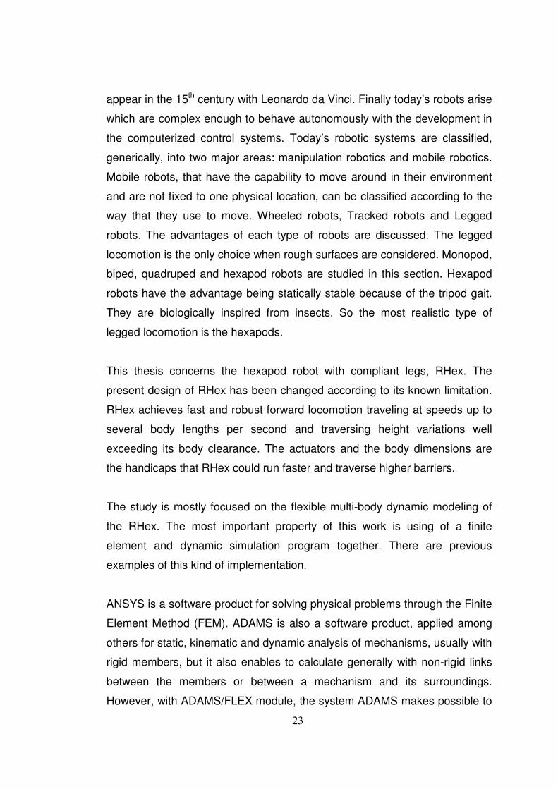
Figure 16 ADAMS Model Figure 17 Experimental Setup
Using this phenomenon the behavior of distribution systems OHV and OHC
are studied by Antonin Potesil and Vaclav Hanzlik. [45] By means of the FEM
and ADAMS models (Figure 16);
• kinematic quantities could be predicted,
25
• loading and stresses of individual parts of the system could be
identified,
• the weight, dimension and the strength characteristic of the parts
could be optimized,
• a cheaper and faster test method is used compared to running the
real experiment (Figure 17).
In the past Finite Element Analysis (FEA) and Multibody System Simulation
(MBS) were two isolated approaches in the field of mechanical system
simulation. While multibody analysis codes focused on the nonlinear
dynamics of entire systems of interconnected rigid bodies, FEA solvers were
used to investigate the elastic/plastic behavior of single deformable
components. In recent years different software products e.g. ADAMS/Flex
have come into the market that utilize sub-structuring techniques to combine
the benefits of both FEA and MBS. In the field of multibody system simulation
the intention is the realistic representation of component level flexibility. For
FEA purposes this method can be used to derive complex dynamic loading
conditions for these flexible components, which cannot be done manually in
general. Particularly in the field of finite element based structural
optimization, the formulation of realistic boundary and loading conditions is of
vital interest as these significantly influence the final design. Since structural
optimization implies a change of the components shape (i.e. the mass
distribution) during each iterations, the dynamic inertia loads and the
components’ dynamical properties will change accordingly. In traditional
structural optimization, usually constant loads and boundary conditions are
used. A coupled MBS-FEA optimization approach opens up the possibility to
take these iteration dependent load changes into account while optimizing
the component. This leads to an improved design of the considered
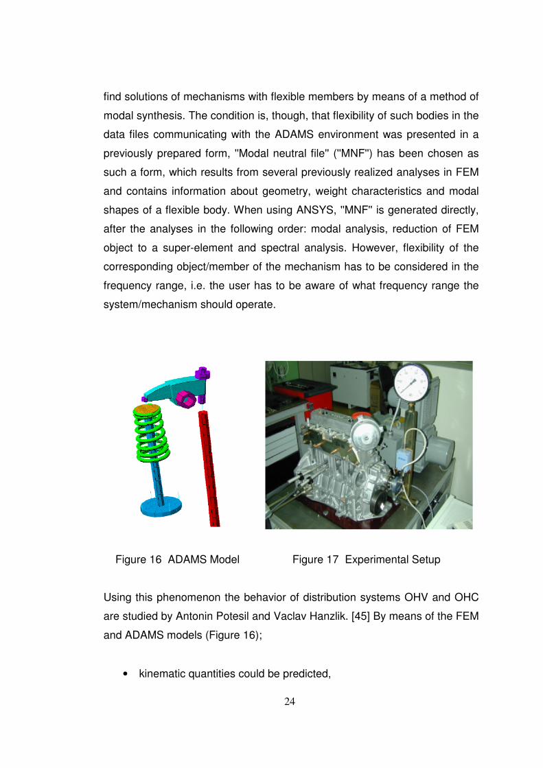
component and shorter product development time. Another study was
performed by Albers, A. [46] about shape optimization of a simple crank drive
mechanism (Figure 18) using this FEM-MBS optimization approach. In this
study, the structural optimization of dynamically loaded finite element flexible
26
components embedded in a multibody system by means of an automated
coupling of MSC.ADAMS with MSC.NASTRAN Sol200 as optimizer is
described.
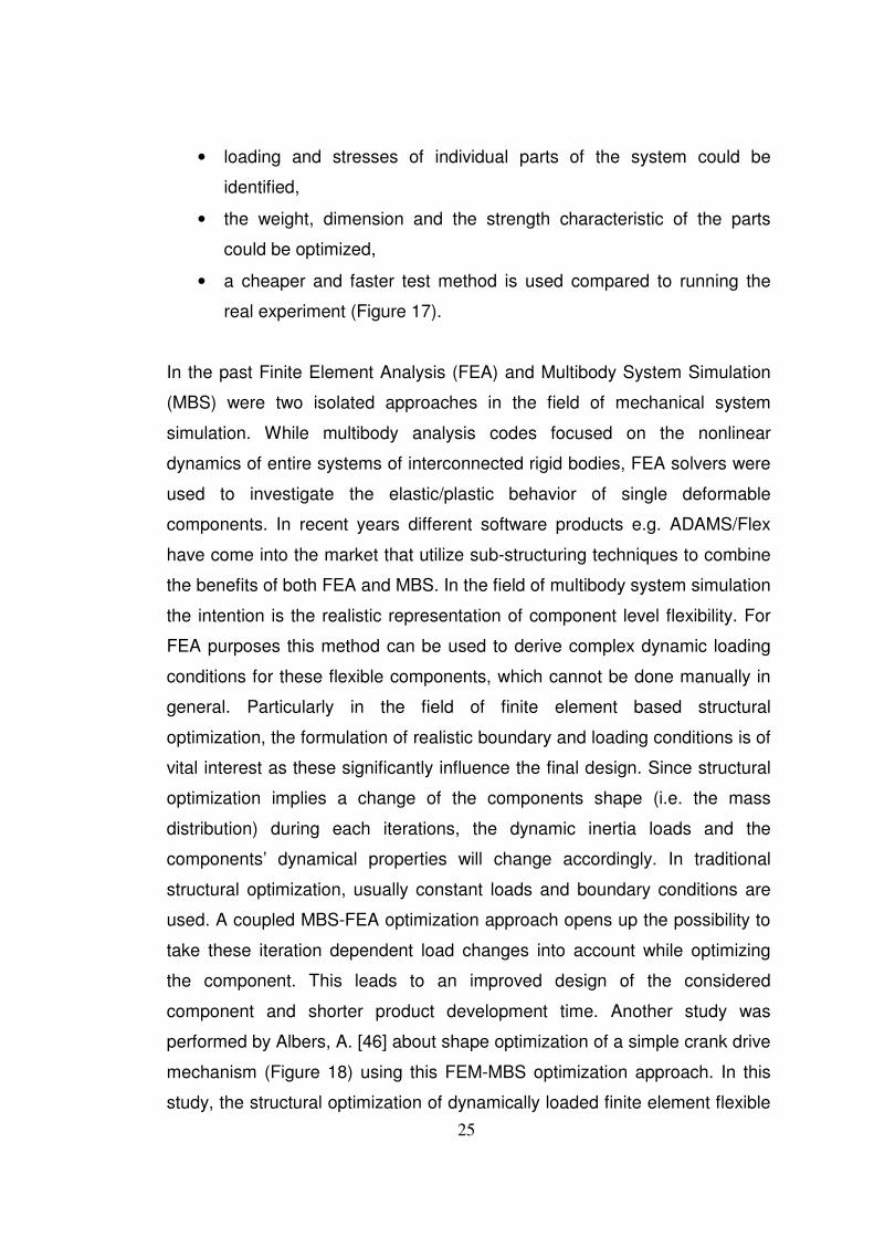
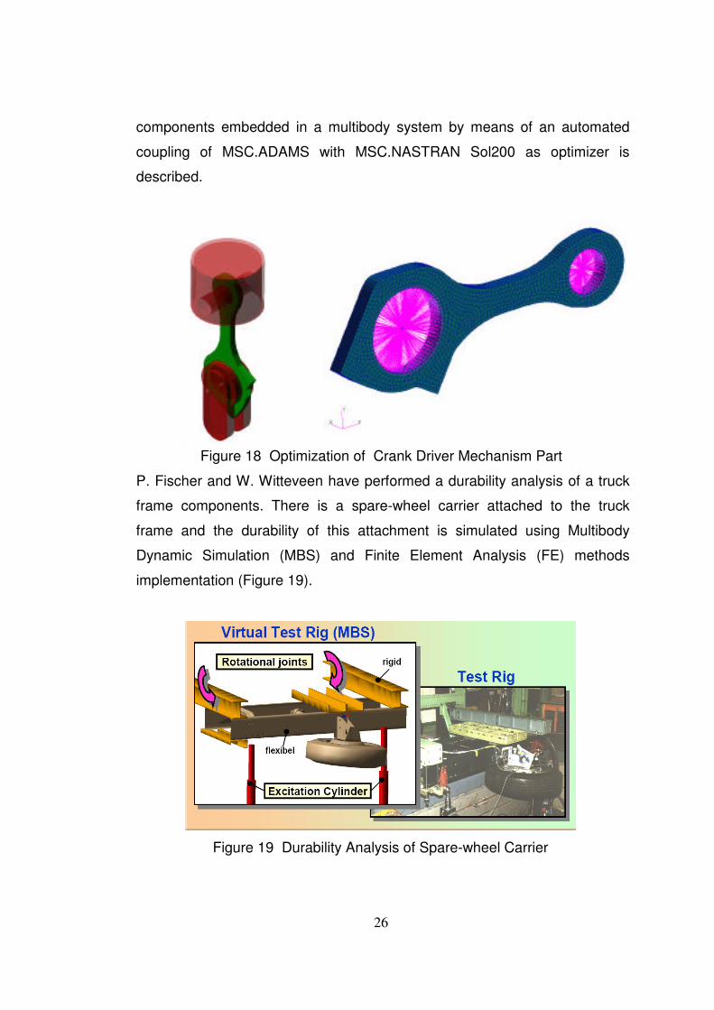
Figure 18 Optimization of Crank Driver Mechanism Part
P. Fischer and W. Witteveen have performed a durability analysis of a truck
frame components. There is a spare-wheel carrier attached to the truck
frame and the durability of this attachment is simulated using Multibody
Dynamic Simulation (MBS) and Finite Element Analysis (FE) methods
implementation (Figure 19).
Figure 19 Durability Analysis of Spare-wheel Carrier
27
The idea is the same. First the finite element analysis is performed and the
deformations are calculated to the corresponding loads. Then the shapes
and positions of the parts are updated in the multibody simulation according
to the FE analysis. After performing the dynamic simulation with the updated
information the new calculated loads are transferred to the FE analysis.
Same procedure repeats itself until a failure is detected.
Although in the past MBS and FE analysis were different approaches,
nowadays they are used together to perform studies about flexible multibody
dynamic systems. The focus of this thesis is to build a virtual prototype of
RHex which is a multibody system with six compliant legs. MSC ADAMS
software is used for dynamic simulation of the robot, the finite element model
of the flexible legs is created with MSC Patran and the useful MNF file is built
with MSC Nastran. The details of this study and implementation of these
programs are discussed in the following section.
28
CHAPTER 2
2. MECHANICAL DESIGN OF RHEX
RHex is primarily a research platform that is based on over five years of
previous research. The purpose of the present task is to design the next
iteration of the successful RHex hexapod mobile robot platform. Previous
versions of RHex successively completed the primary mission which is to
operate on rugged, fractured terrain through statically and dynamically stable
gaits while stability of locomotion is preserved. Although RHex meets the
basic requirements to accomplish the primary task, there are lots of known
limitations or points that could be improved. Modularity of the design is of
utmost importance in order to give the ability to experiment with design
choices concerning electrical system, sensors, actuators, computational
hardware as well as body mechanical design features. Therefore mechanical
parts are designed such that the components could be easily detached and
changed or at least reachable without demounting another part. This valuable
information illuminate the way for the next mechanical design iteration. In the
following section, mechanical design optimizations of RHex are discussed.
2.1 Overall Description of the Design
The platform RHex consist of base frame, crash frame, motor mounting
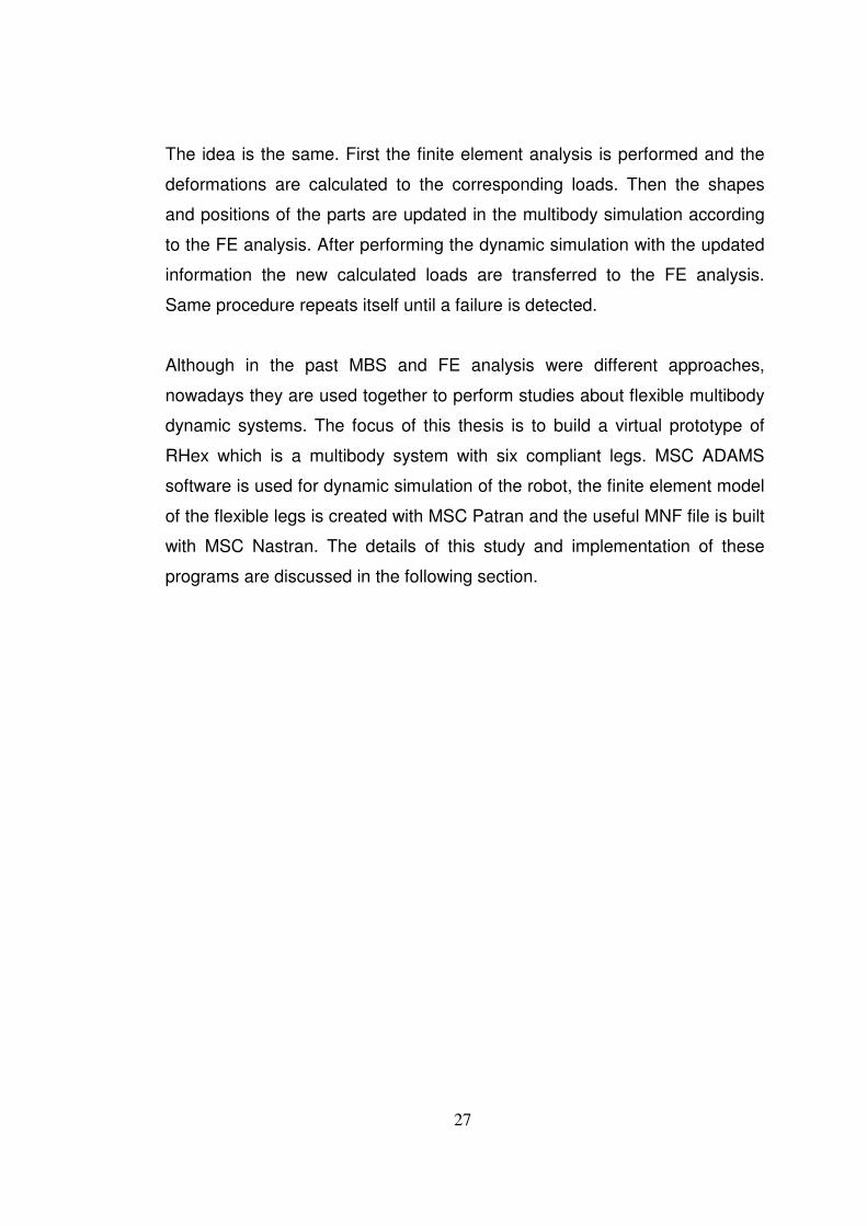
parts, interior mounting parts, legs and leg mounting parts. The base and
crash frame form the main body of RHex (Figure 20) with the base frame
being the main carrier of critical drive-train components. The six motors and
gearboxes are mounted hence to the base frame. This frame has three cross
members each carrying a pair of motor and gear box combination. Motor
mounting parts consist of two parts, a ball bearing and a shaft collar. This
sub-assembly is held together by four screws to the motor body and is
29
mounted with two M3 screws to the end of the cross members of the base
frame.
Figure 20 The base and crash frame assembly
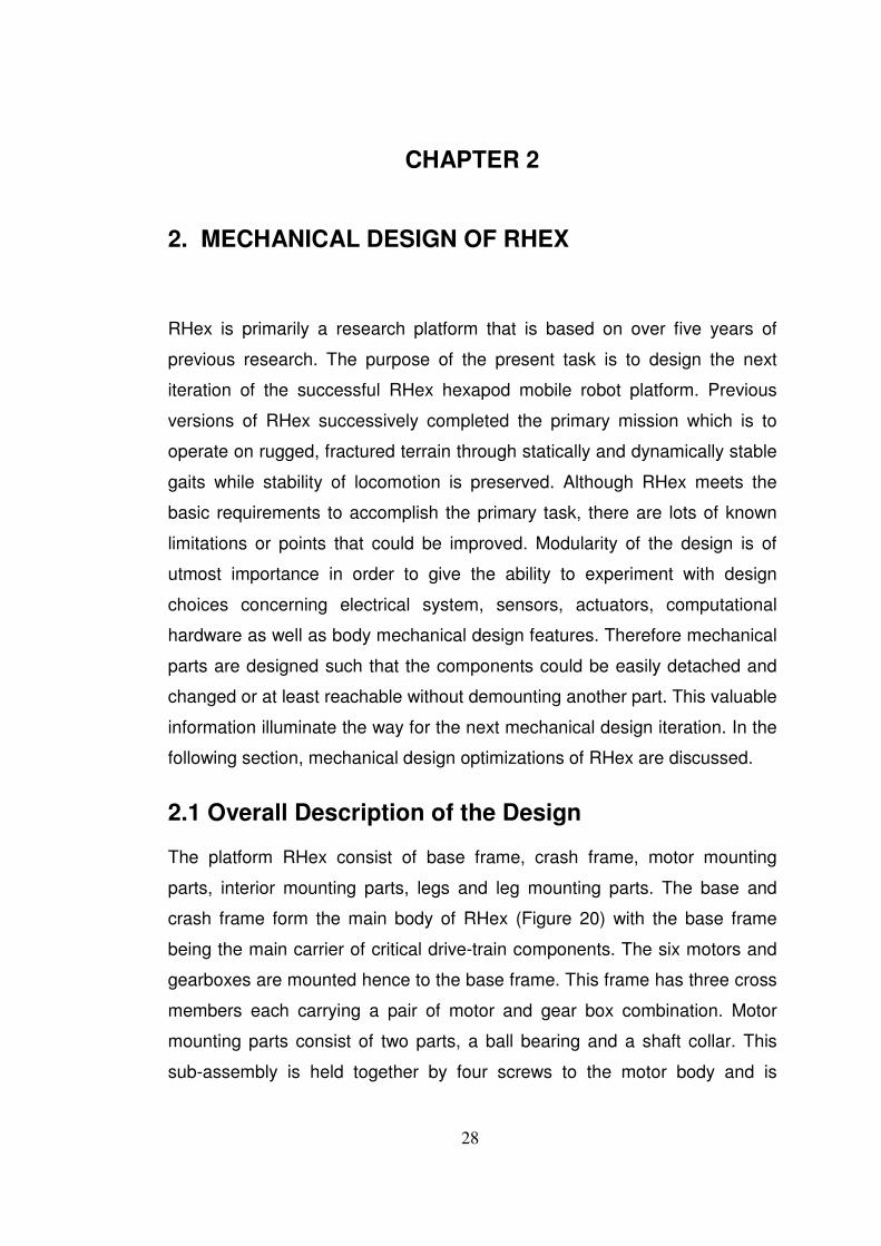
In addition to the motors and gearboxes battery packs are also carried by the
base frame. For the time being three battery packs are used and each are
mounted below the cross member. Figure 21 shows clearly the produced
motor assemblies under which the batteries will be carried.
Figure 21 The photograph of the main body of Rhex (base and crash frame)
with motor and gearbox assemblies.
30
2.2. Crash Frame
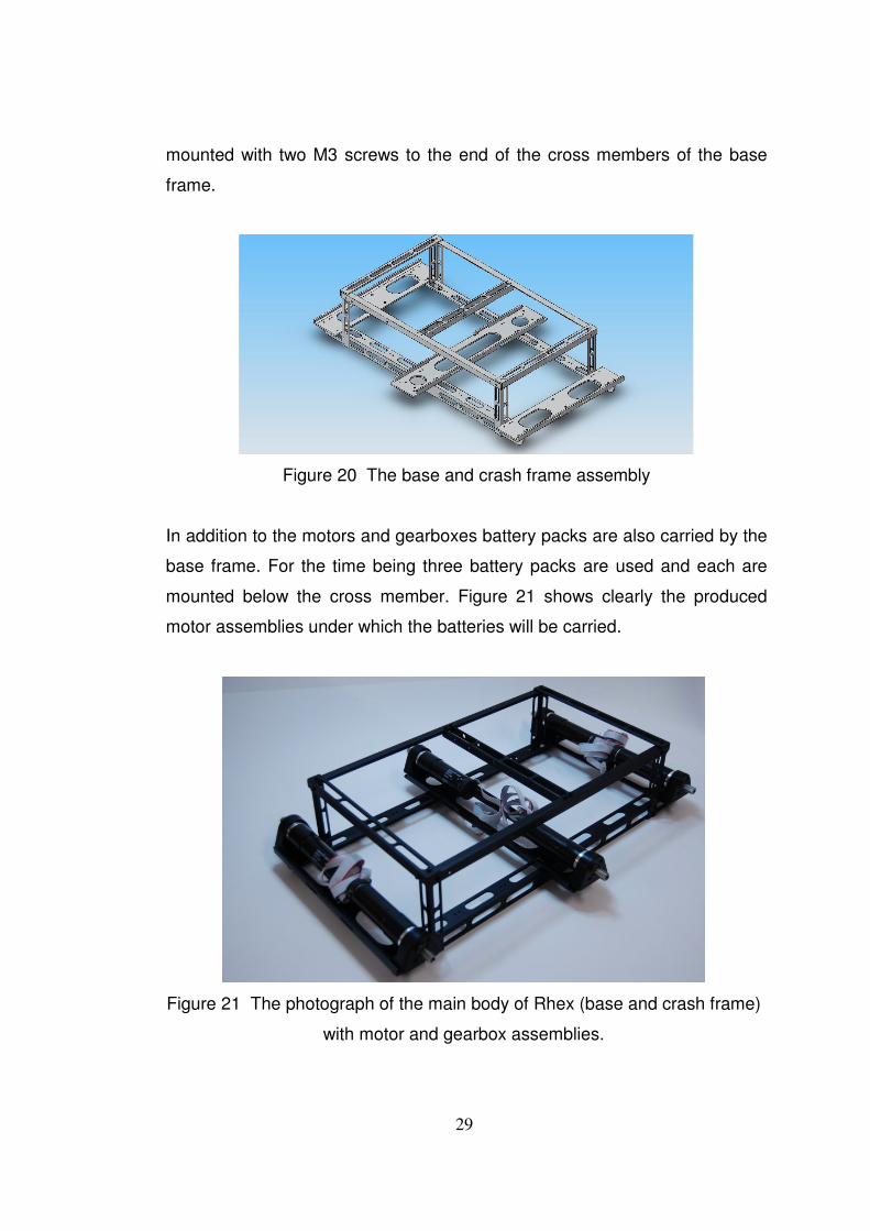
The crash frame, as the name implies, is protecting the interior electronic
parts. The experimental results with the previous version of RHex showed
that crash frame could be damaged or even broken when the robot rolls over.
Therefore this frame should be both structurally protective and modular. In
case of a crash, parts should be easily exchangeable. The crash frame
consists of nine parts as could be seen from the Figure 22.
Figure 22 The crash frame of RHex
The design is updated such that the whole mechanical system is modular.
One mechanical part or an electronics component should be reachable and
could be detached without demounting any other component. Keeping this
principle in mind, all the mechanical parts are reviewed and subjected to
slight changes to accomplish this criterion. The previous experimental data
and outdoor run results are used to perform this study. One of the examples
of this design modification is with the motor mounting parts. The mounting
holes of this sub-assembly used to attach it to the base frame could not be
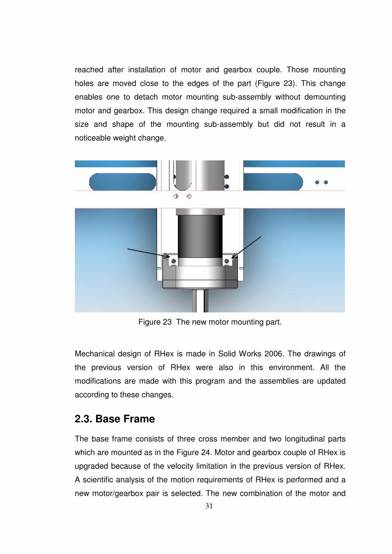
31
reached after installation of motor and gearbox couple. Those mounting
holes are moved close to the edges of the part (Figure 23). This change
enables one to detach motor mounting sub-assembly without demounting
motor and gearbox. This design change required a small modification in the
size and shape of the mounting sub-assembly but did not result in a
noticeable weight change.
Figure 23 The new motor mounting part.
Mechanical design of RHex is made in Solid Works 2006. The drawings of
the previous version of RHex were also in this environment. All the
modifications are made with this program and the assemblies are updated
according to these changes.
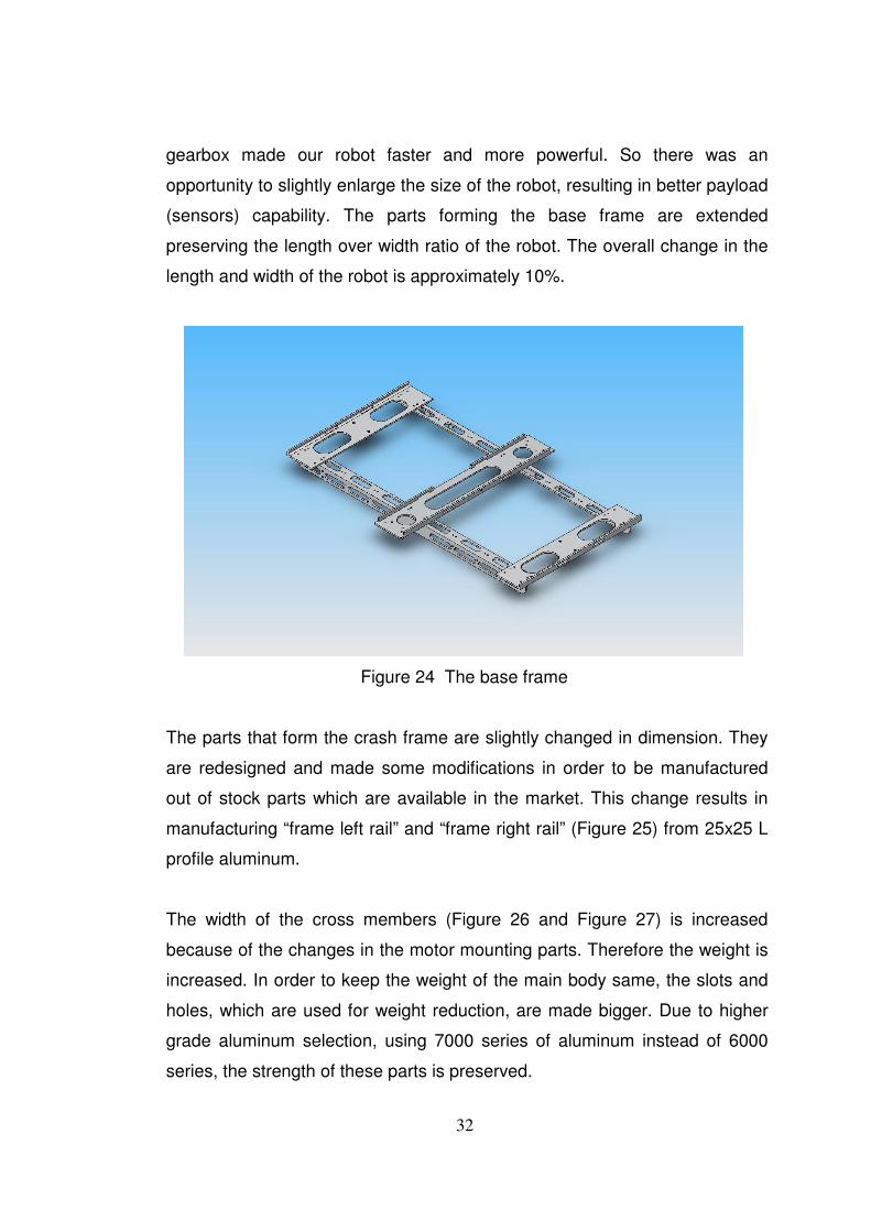
2.3. Base Frame
The base frame consists of three cross member and two longitudinal parts
which are mounted as in the Figure 24. Motor and gearbox couple of RHex is
upgraded because of the velocity limitation in the previous version of RHex.
A scientific analysis of the motion requirements of RHex is performed and a
new motor/gearbox pair is selected. The new combination of the motor and
32
gearbox made our robot faster and more powerful. So there was an
opportunity to slightly enlarge the size of the robot, resulting in better payload
(sensors) capability. The parts forming the base frame are extended
preserving the length over width ratio of the robot. The overall change in the
length and width of the robot is approximately 10%.
Figure 24 The base frame
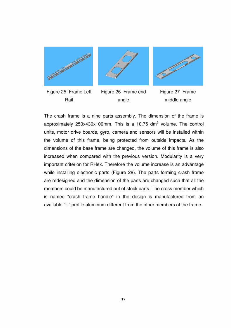
The parts that form the crash frame are slightly changed in dimension. They
are redesigned and made some modifications in order to be manufactured
out of stock parts which are available in the market. This change results in
manufacturing “frame left rail” and “frame right rail” (Figure 25) from 25x25 L
profile aluminum.
The width of the cross members (Figure 26 and Figure 27) is increased
because of the changes in the motor mounting parts. Therefore the weight is
increased. In order to keep the weight of the main body same, the slots and
holes, which are used for weight reduction, are made bigger. Due to higher
grade aluminum selection, using 7000 series of aluminum instead of 6000
series, the strength of these parts is preserved.
33
Figure 25 Frame Left
Rail
Figure 26 Frame end
angle
Figure 27 Frame
middle angle
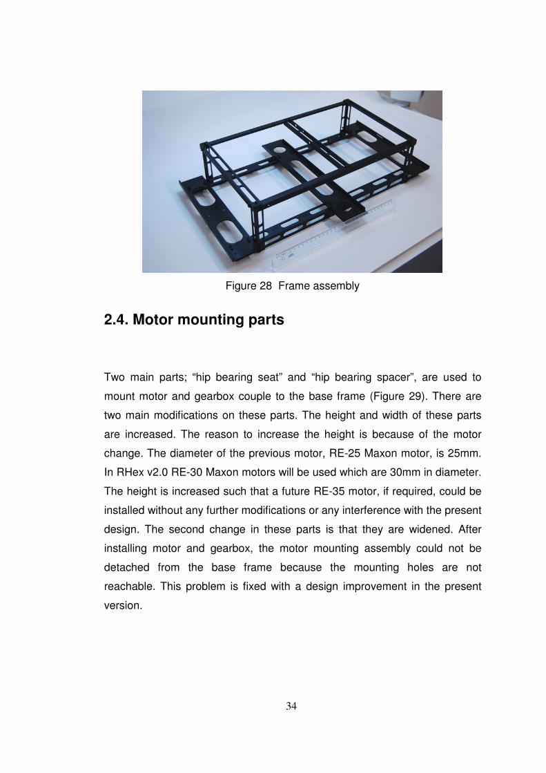
The crash frame is a nine parts assembly. The dimension of the frame is
approximately 250x430x100mm. This is a 10.75 dm3 volume. The control
units, motor drive boards, gyro, camera and sensors will be installed within
the volume of this frame, being protected from outside impacts. As the
dimensions of the base frame are changed, the volume of this frame is also
increased when compared with the previous version. Modularity is a very
important criterion for RHex. Therefore the volume increase is an advantage
while installing electronic parts (Figure 28). The parts forming crash frame
are redesigned and the dimension of the parts are changed such that all the
members could be manufactured out of stock parts. The cross member which
is named “crash frame handle” in the design is manufactured from an
available “U” profile aluminum different from the other members of the frame.
34
Figure 28 Frame assembly
2.4. Motor mounting parts
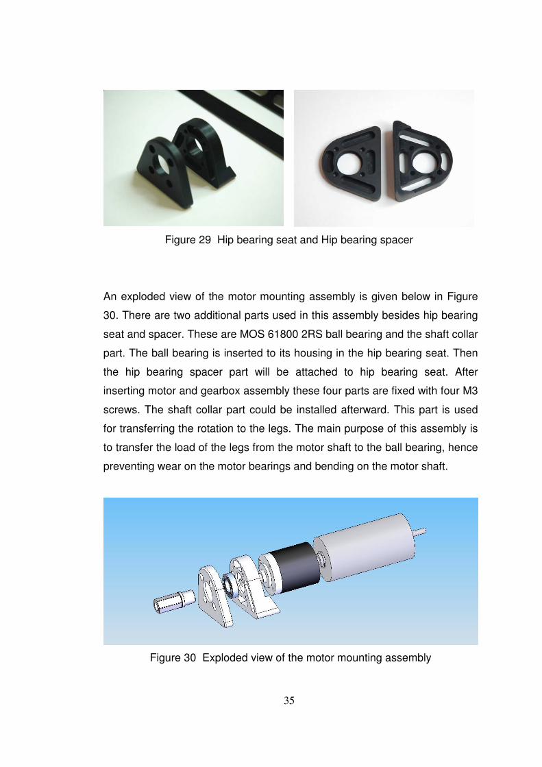
Two main parts; “hip bearing seat” and “hip bearing spacer”, are used to
mount motor and gearbox couple to the base frame (Figure 29). There are
two main modifications on these parts. The height and width of these parts
are increased. The reason to increase the height is because of the motor
change. The diameter of the previous motor, RE-25 Maxon motor, is 25mm.
In RHex v2.0 RE-30 Maxon motors will be used which are 30mm in diameter.
The height is increased such that a future RE-35 motor, if required, could be
installed without any further modifications or any interference with the present
design. The second change in these parts is that they are widened. After
installing motor and gearbox, the motor mounting assembly could not be
detached from the base frame because the mounting holes are not
reachable. This problem is fixed with a design improvement in the present
version.
35
Figure 29 Hip bearing seat and Hip bearing spacer
An exploded view of the motor mounting assembly is given below in Figure
30. There are two additional parts used in this assembly besides hip bearing
seat and spacer. These are MOS 61800 2RS ball bearing and the shaft collar
part. The ball bearing is inserted to its housing in the hip bearing seat. Then
the hip bearing spacer part will be attached to hip bearing seat. After
inserting motor and gearbox assembly these four parts are fixed with four M3
screws. The shaft collar part could be installed afterward. This part is used
for transferring the rotation to the legs. The main purpose of this assembly is
to transfer the load of the legs from the motor shaft to the ball bearing, hence
preventing wear on the motor bearings and bending on the motor shaft.
Figure 30 Exploded view of the motor mounting assembly
36
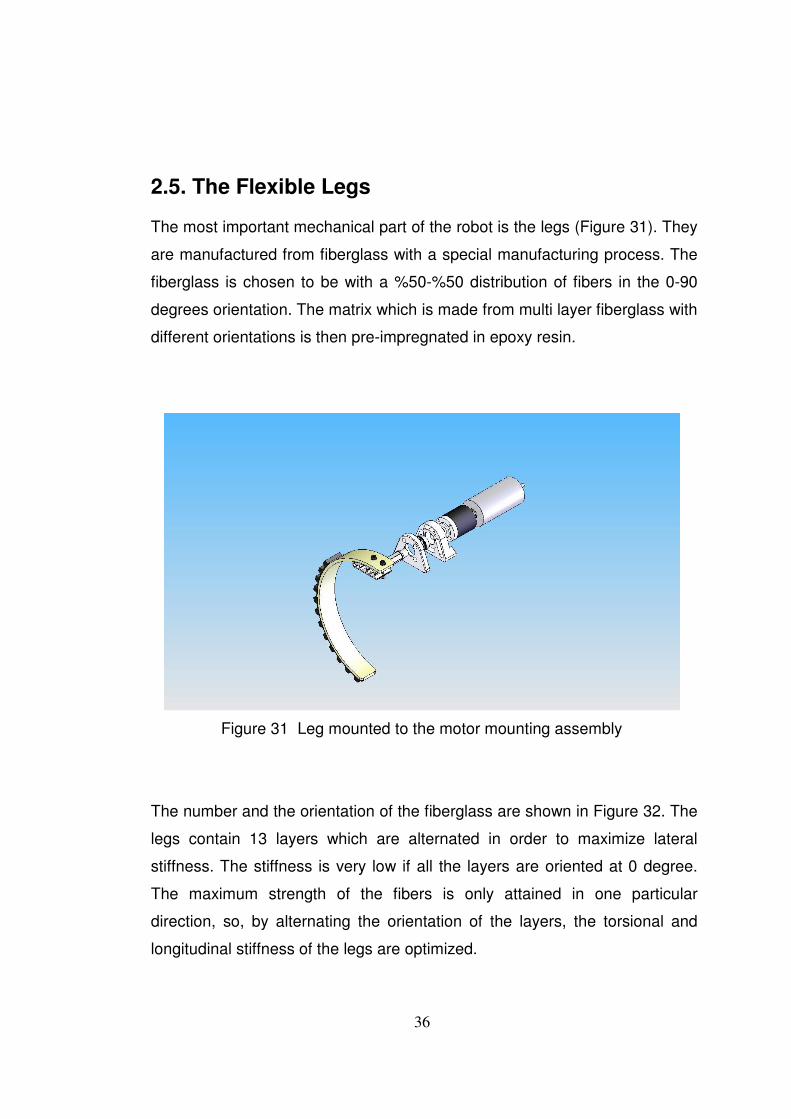
2.5. The Flexible Legs
The most important mechanical part of the robot is the legs (Figure 31). They
are manufactured from fiberglass with a special manufacturing process. The
fiberglass is chosen to be with a %50-%50 distribution of fibers in the 0-90
degrees orientation. The matrix which is made from multi layer fiberglass with
different orientations is then pre-impregnated in epoxy resin.
Figure 31 Leg mounted to the motor mounting assembly
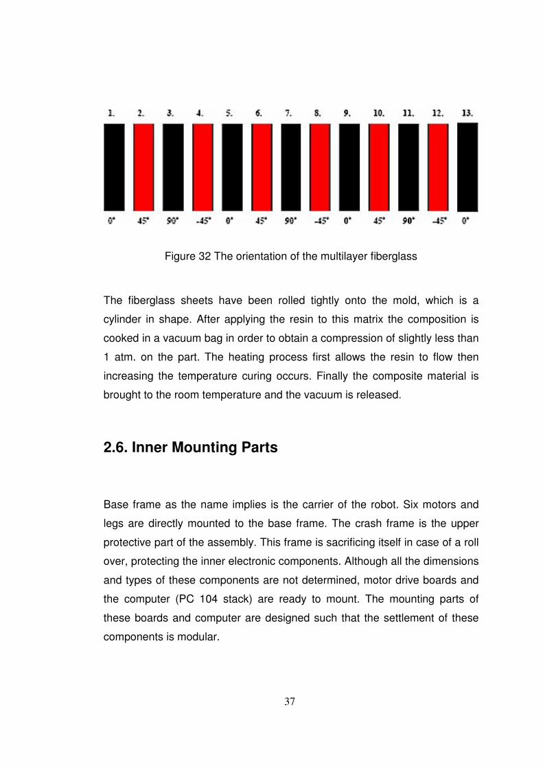
The number and the orientation of the fiberglass are shown in Figure 32. The
legs contain 13 layers which are alternated in order to maximize lateral
stiffness. The stiffness is very low if all the layers are oriented at 0 degree.
The maximum strength of the fibers is only attained in one particular
direction, so, by alternating the orientation of the layers, the torsional and
longitudinal stiffness of the legs are optimized.
37
Figure 32 The orientation of the multilayer fiberglass
The fiberglass sheets have been rolled tightly onto the mold, which is a
cylinder in shape. After applying the resin to this matrix the composition is
cooked in a vacuum bag in order to obtain a compression of slightly less than
1 atm. on the part. The heating process first allows the resin to flow then
increasing the temperature curing occurs. Finally the composite material is
brought to the room temperature and the vacuum is released.
2.6. Inner Mounting Parts
Base frame as the name implies is the carrier of the robot. Six motors and
legs are directly mounted to the base frame. The crash frame is the upper
protective part of the assembly. This frame is sacrificing itself in case of a roll
over, protecting the inner electronic components. Although all the dimensions
and types of these components are not determined, motor drive boards and
the computer (PC 104 stack) are ready to mount. The mounting parts of
these boards and computer are designed such that the settlement of these
components is modular.
38
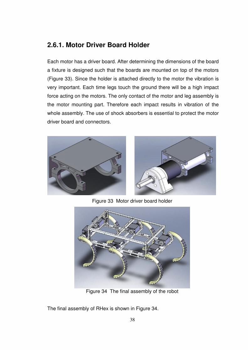
2.6.1. Motor Driver Board Holder
Each motor has a driver board. After determining the dimensions of the board
a fixture is designed such that the boards are mounted on top of the motors
(Figure 33). Since the holder is attached directly to the motor the vibration is
very important. Each time legs touch the ground there will be a high impact
force acting on the motors. The only contact of the motor and leg assembly is
the motor mounting part. Therefore each impact results in vibration of the
whole assembly. The use of shock absorbers is essential to protect the motor
driver board and connectors.
Figure 33 Motor driver board holder
Figure 34 The final assembly of the robot
The final assembly of RHex is shown in Figure 34.
39
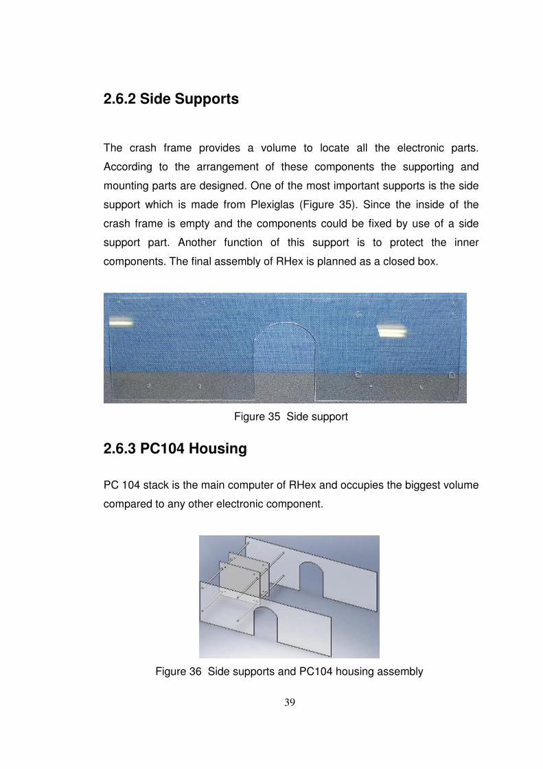
2.6.2 Side Supports
The crash frame provides a volume to locate all the electronic parts.
According to the arrangement of these components the supporting and
mounting parts are designed. One of the most important supports is the side
support which is made from Plexiglas (Figure 35). Since the inside of the
crash frame is empty and the components could be fixed by use of a side
support part. Another function of this support is to protect the inner
components. The final assembly of RHex is planned as a closed box.
Figure 35 Side support
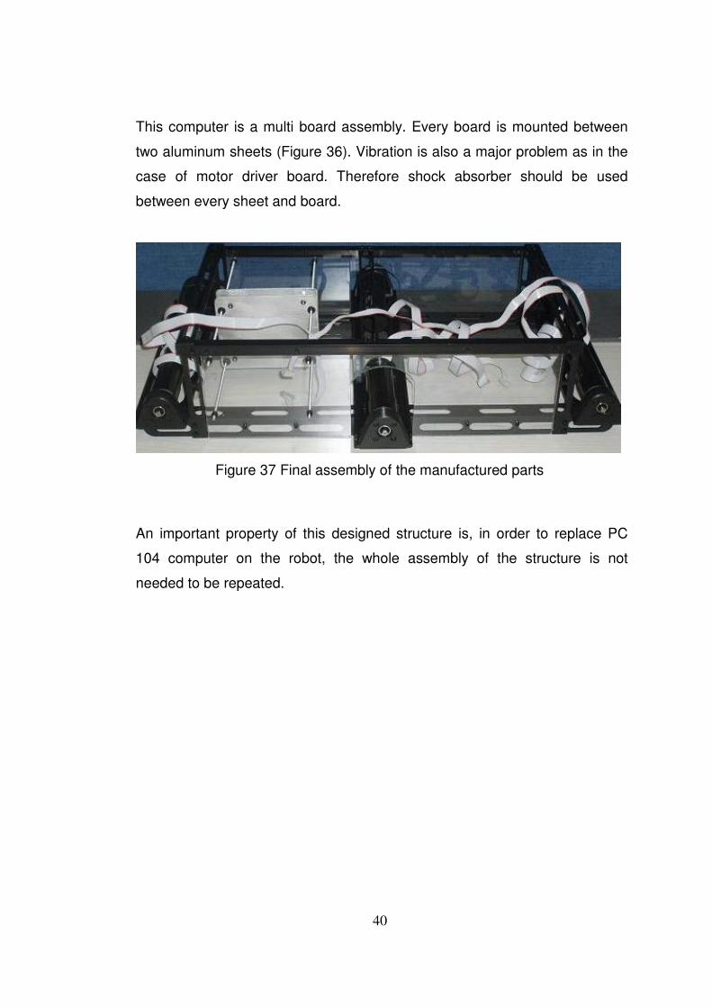
2.6.3 PC104 Housing
PC 104 stack is the main computer of RHex and occupies the biggest volume
compared to any other electronic component.
Figure 36 Side supports and PC104 housing assembly
40
This computer is a multi board assembly. Every board is mounted between
two aluminum sheets (Figure 36). Vibration is also a major problem as in the
case of motor driver board. Therefore shock absorber should be used
between every sheet and board.
Figure 37 Final assembly of the manufactured parts
An important property of this designed structure is, in order to replace PC
104 computer on the robot, the whole assembly of the structure is not
needed to be repeated.
41
CHAPTER 3
FLEXIBLE MULTIBODY DYNAMIC SIMULATION
3.1. Motivation
Multibody Dynamics is an exciting area of Computational Mechanics, which
merges and blends various disciplines such as structural dynamics, multi-
physic mechanics, computational mathematics, control theory and computer
science in order to deliver methods and tools for the virtual prototyping of
complex mechanical systems. Multibody dynamics plays today a central role
in the modeling, analysis, simulation and optimization of mechanical systems
in a variety of fields and for a wide range of industrial applications.
The focus of interest in this study is the Rhex robot, which is an autonomous
hexapod robot with compliant legs. It consists of different rigid bodies
assembled together to build base frame and crash frame for the first part. For
the second part six compliant (currently half-circular and made from
composite material) legs are attached to the base frame with a rotating hip
mechanism and are actuated by one motor per leg. The half circular and
flexible legs contribute to the dynamic stability of the robot and act as a
suspension system. So Rhex, being a complex mechanical system, is
modeled in ADAMS software to be able to analyze and optimize the design.
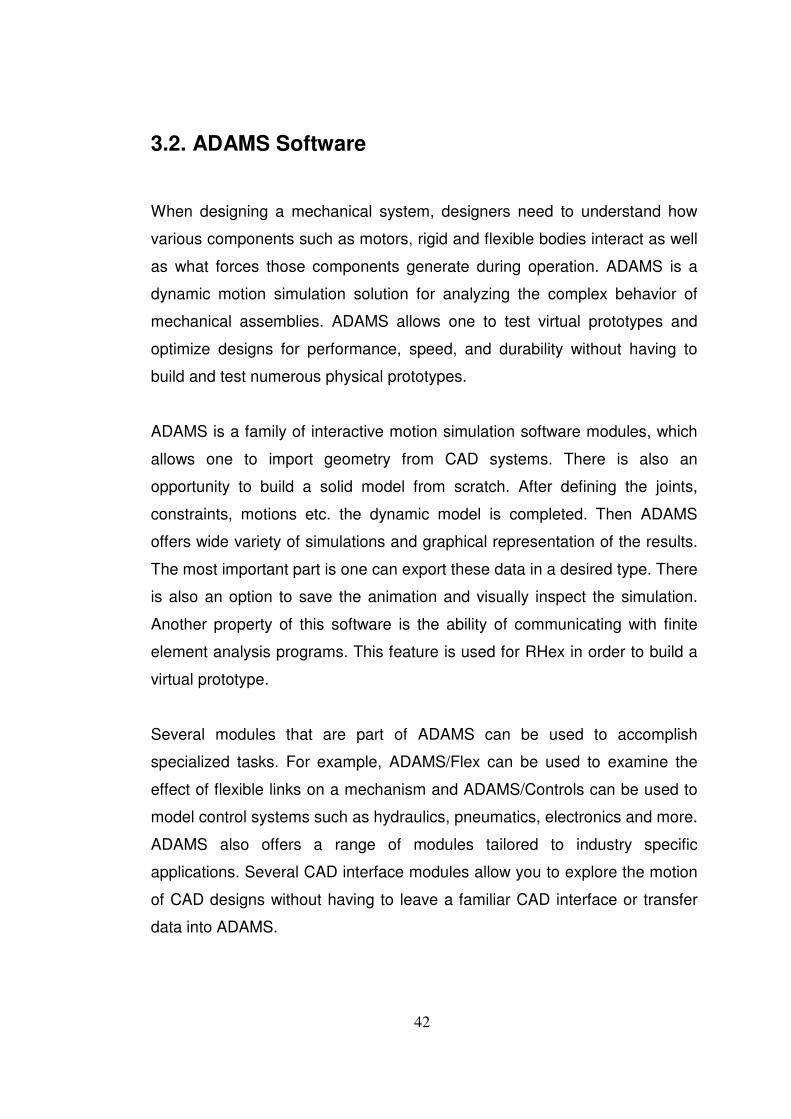
42
3.2. ADAMS Software
When designing a mechanical system, designers need to understand how
various components such as motors, rigid and flexible bodies interact as well
as what forces those components generate during operation. ADAMS is a
dynamic motion simulation solution for analyzing the complex behavior of
mechanical assemblies. ADAMS allows one to test virtual prototypes and
optimize designs for performance, speed, and durability without having to
build and test numerous physical prototypes.
ADAMS is a family of interactive motion simulation software modules, which
allows one to import geometry from CAD systems. There is also an
opportunity to build a solid model from scratch. After defining the joints,
constraints, motions etc. the dynamic model is completed. Then ADAMS
offers wide variety of simulations and graphical representation of the results.
The most important part is one can export these data in a desired type. There
is also an option to save the animation and visually inspect the simulation.
Another property of this software is the ability of communicating with finite
element analysis programs. This feature is used for RHex in order to build a
virtual prototype.
Several modules that are part of ADAMS can be used to accomplish
specialized tasks. For example, ADAMS/Flex can be used to examine the
effect of flexible links on a mechanism and ADAMS/Controls can be used to
model control systems such as hydraulics, pneumatics, electronics and more.
ADAMS also offers a range of modules tailored to industry specific
applications. Several CAD interface modules allow you to explore the motion
of CAD designs without having to leave a familiar CAD interface or transfer
data into ADAMS.
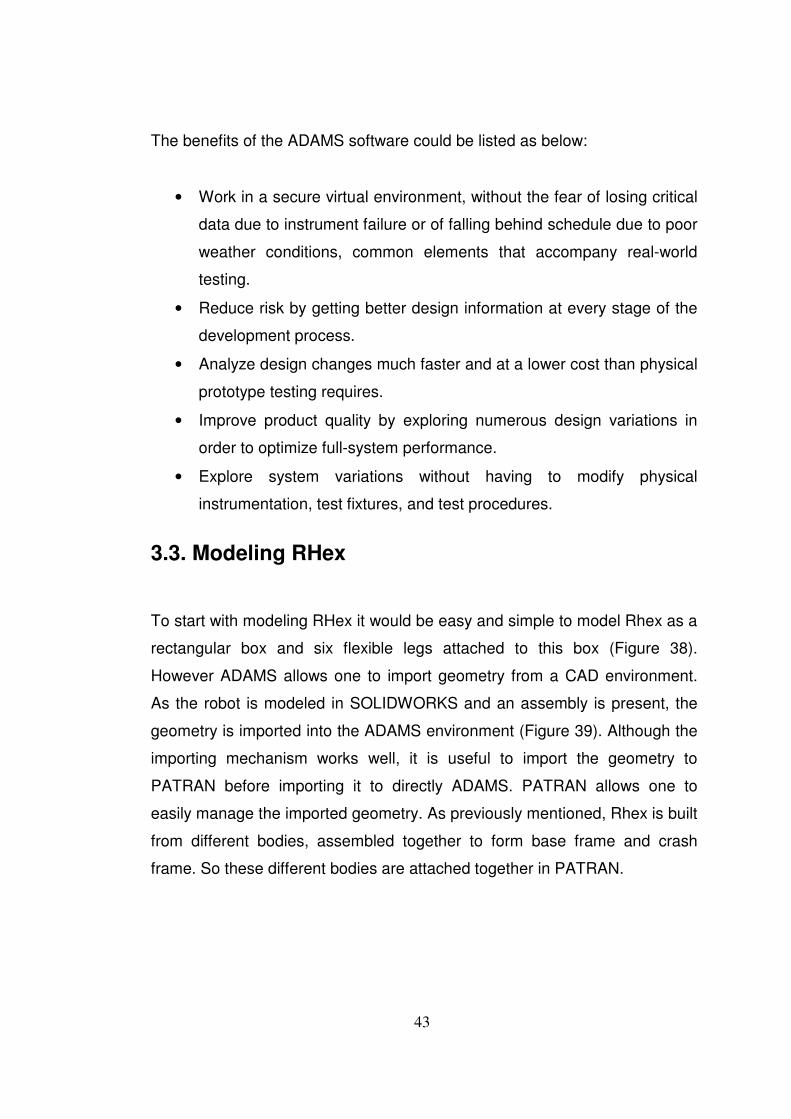
43
The benefits of the ADAMS software could be listed as below:
• Work in a secure virtual environment, without the fear of losing critical
data due to instrument failure or of falling behind schedule due to poor
weather conditions, common elements that accompany real-world
testing.
• Reduce risk by getting better design information at every stage of the
development process.
• Analyze design changes much faster and at a lower cost than physical
prototype testing requires.
• Improve product quality by exploring numerous design variations in
order to optimize full-system performance.
• Explore system variations without having to modify physical
instrumentation, test fixtures, and test procedures.
3.3. Modeling RHex
To start with modeling RHex it would be easy and simple to model Rhex as a
rectangular box and six flexible legs attached to this box (Figure 38).
However ADAMS allows one to import geometry from a CAD environment.
As the robot is modeled in SOLIDWORKS and an assembly is present, the
geometry is imported into the ADAMS environment (Figure 39). Although the
importing mechanism works well, it is useful to import the geometry to
PATRAN before importing it to directly ADAMS. PATRAN allows one to
easily manage the imported geometry. As previously mentioned, Rhex is built
from different bodies, assembled together to form base frame and crash
frame. So these different bodies are attached together in PATRAN.
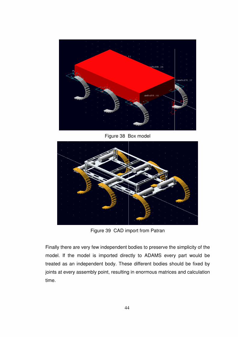
44
Figure 38 Box model
Figure 39 CAD import from Patran
Finally there are very few independent bodies to preserve the simplicity of the
model. If the model is imported directly to ADAMS every part would be
treated as an independent body. These different bodies should be fixed by
joints at every assembly point, resulting in enormous matrices and calculation
time.
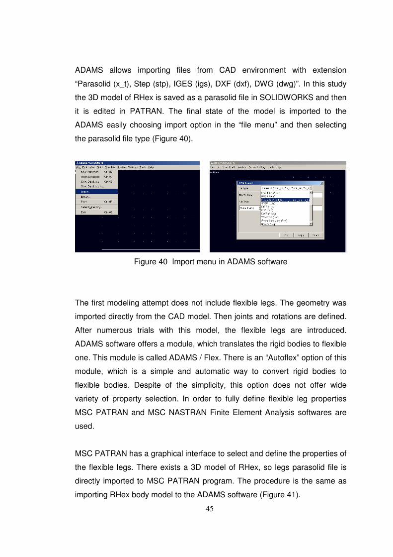
45
ADAMS allows importing files from CAD environment with extension
“Parasolid (x_t), Step (stp), IGES (igs), DXF (dxf), DWG (dwg)”. In this study
the 3D model of RHex is saved as a parasolid file in SOLIDWORKS and then
it is edited in PATRAN. The final state of the model is imported to the
ADAMS easily choosing import option in the “file menu” and then selecting
the parasolid file type (Figure 40).
Figure 40 Import menu in ADAMS software
The first modeling attempt does not include flexible legs. The geometry was
imported directly from the CAD model. Then joints and rotations are defined.
After numerous trials with this model, the flexible legs are introduced.
ADAMS software offers a module, which translates the rigid bodies to flexible
one. This module is called ADAMS / Flex. There is an “Autoflex” option of this
module, which is a simple and automatic way to convert rigid bodies to
flexible bodies. Despite of the simplicity, this option does not offer wide
variety of property selection. In order to fully define flexible leg properties
MSC PATRAN and MSC NASTRAN Finite Element Analysis softwares are
used.
MSC PATRAN has a graphical interface to select and define the properties of
the flexible legs. There exists a 3D model of RHex, so legs parasolid file is
directly imported to MSC PATRAN program. The procedure is the same as
importing RHex body model to the ADAMS software (Figure 41).
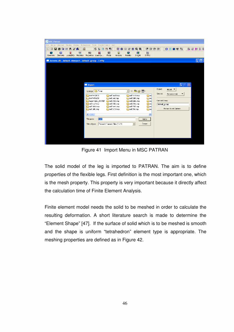
46
Figure 41 Import Menu in MSC PATRAN
The solid model of the leg is imported to PATRAN. The aim is to define
properties of the flexible legs. First definition is the most important one, which
is the mesh property. This property is very important because it directly affect
the calculation time of Finite Element Analysis.
Finite element model needs the solid to be meshed in order to calculate the
resulting deformation. A short literature search is made to determine the
“Element Shape” [47]. If the surface of solid which is to be meshed is smooth
and the shape is uniform “tetrahedron” element type is appropriate. The
meshing properties are defined as in Figure 42.
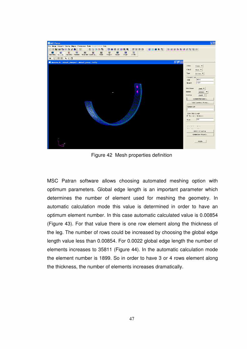
47
Figure 42 Mesh properties definition
MSC Patran software allows choosing automated meshing option with
optimum parameters. Global edge length is an important parameter which
determines the number of element used for meshing the geometry. In
automatic calculation mode this value is determined in order to have an
optimum element number. In this case automatic calculated value is 0.00854
(Figure 43). For that value there is one row element along the thickness of
the leg. The number of rows could be increased by choosing the global edge
length value less than 0.00854. For 0.0022 global edge length the number of
elements increases to 35811 (Figure 44). In the automatic calculation mode
the element number is 1899. So in order to have 3 or 4 rows element along
the thickness, the number of elements increases dramatically.
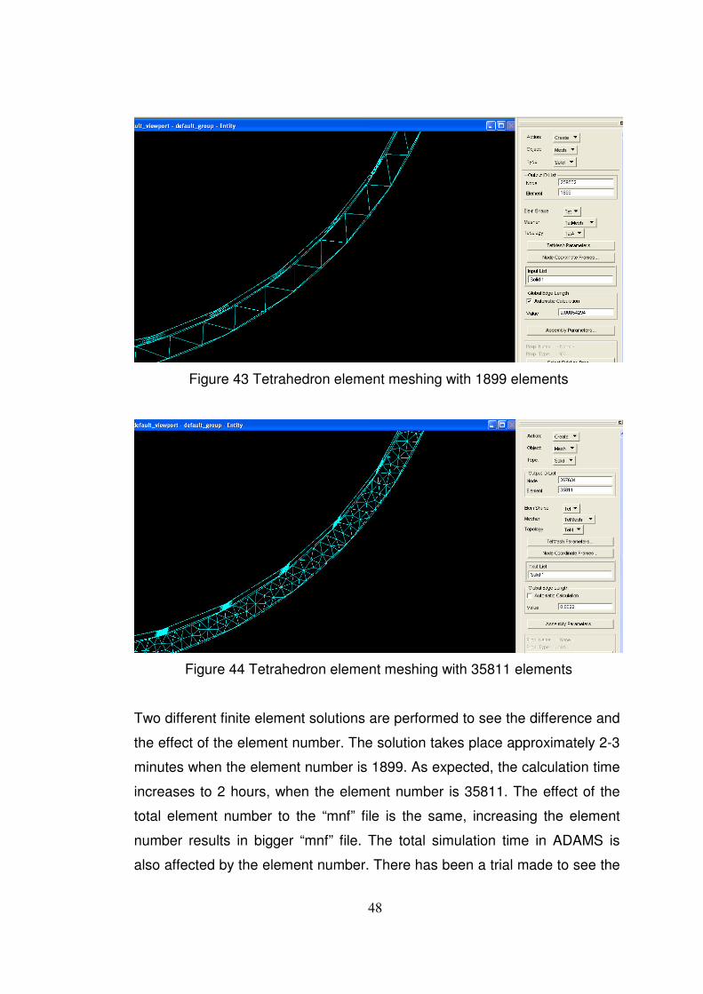
48
Figure 43 Tetrahedron element meshing with 1899 elements
Figure 44 Tetrahedron element meshing with 35811 elements
Two different finite element solutions are performed to see the difference and
the effect of the element number. The solution takes place approximately 2-3
minutes when the element number is 1899. As expected, the calculation time
increases to 2 hours, when the element number is 35811. The effect of the
total element number to the “mnf” file is the same, increasing the element
number results in bigger “mnf” file. The total simulation time in ADAMS is
also affected by the element number. There has been a trial made to see the
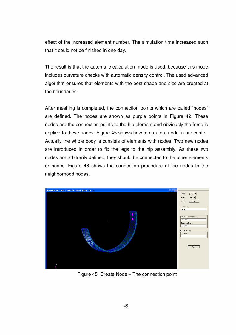
49
effect of the increased element number. The simulation time increased such
that it could not be finished in one day.
The result is that the automatic calculation mode is used, because this mode
includes curvature checks with automatic density control. The used advanced
algorithm ensures that elements with the best shape and size are created at
the boundaries.
After meshing is completed, the connection points which are called “nodes”
are defined. The nodes are shown as purple points in Figure 42. These
nodes are the connection points to the hip element and obviously the force is
applied to these nodes. Figure 45 shows how to create a node in arc center.
Actually the whole body is consists of elements with nodes. Two new nodes
are introduced in order to fix the legs to the hip assembly. As these two
nodes are arbitrarily defined, they should be connected to the other elements
or nodes. Figure 46 shows the connection procedure of the nodes to the
neighborhood nodes.
Figure 45 Create Node – The connection point
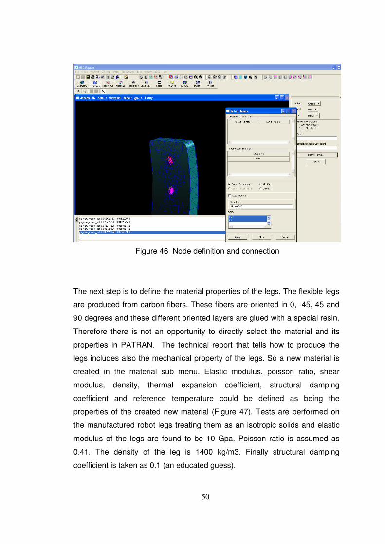
50
Figure 46 Node definition and connection
The next step is to define the material properties of the legs. The flexible legs
are produced from carbon fibers. These fibers are oriented in 0, -45, 45 and
90 degrees and these different oriented layers are glued with a special resin.
Therefore there is not an opportunity to directly select the material and its
properties in PATRAN. The technical report that tells how to produce the
legs includes also the mechanical property of the legs. So a new material is
created in the material sub menu. Elastic modulus, poisson ratio, shear
modulus, density, thermal expansion coefficient, structural damping
coefficient and reference temperature could be defined as being the
properties of the created new material (Figure 47). Tests are performed on
the manufactured robot legs treating them as an isotropic solids and elastic
modulus of the legs are found to be 10 Gpa. Poisson ratio is assumed as
0.41. The density of the leg is 1400 kg/m3. Finally structural damping
coefficient is taken as 0.1 (an educated guess).
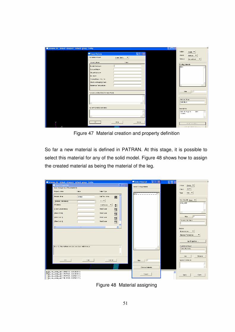
51
Figure 47 Material creation and property definition
So far a new material is defined in PATRAN. At this stage, it is possible to
select this material for any of the solid model. Figure 48 shows how to assign
the created material as being the material of the leg.
Figure 48 Material assigning
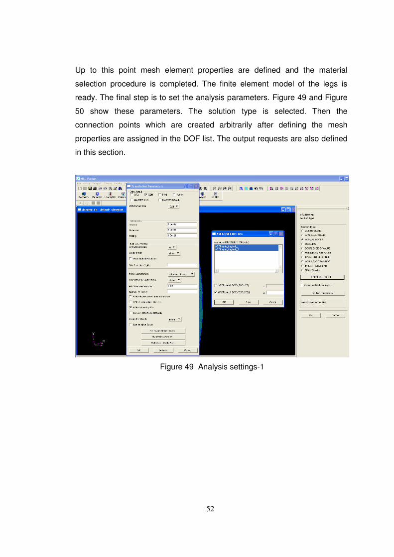
52
Up to this point mesh element properties are defined and the material
selection procedure is completed. The finite element model of the legs is
ready. The final step is to set the analysis parameters. Figure 49 and Figure
50 show these parameters. The solution type is selected. Then the
connection points which are created arbitrarily after defining the mesh
properties are assigned in the DOF list. The output requests are also defined
in this section.
Figure 49 Analysis settings-1
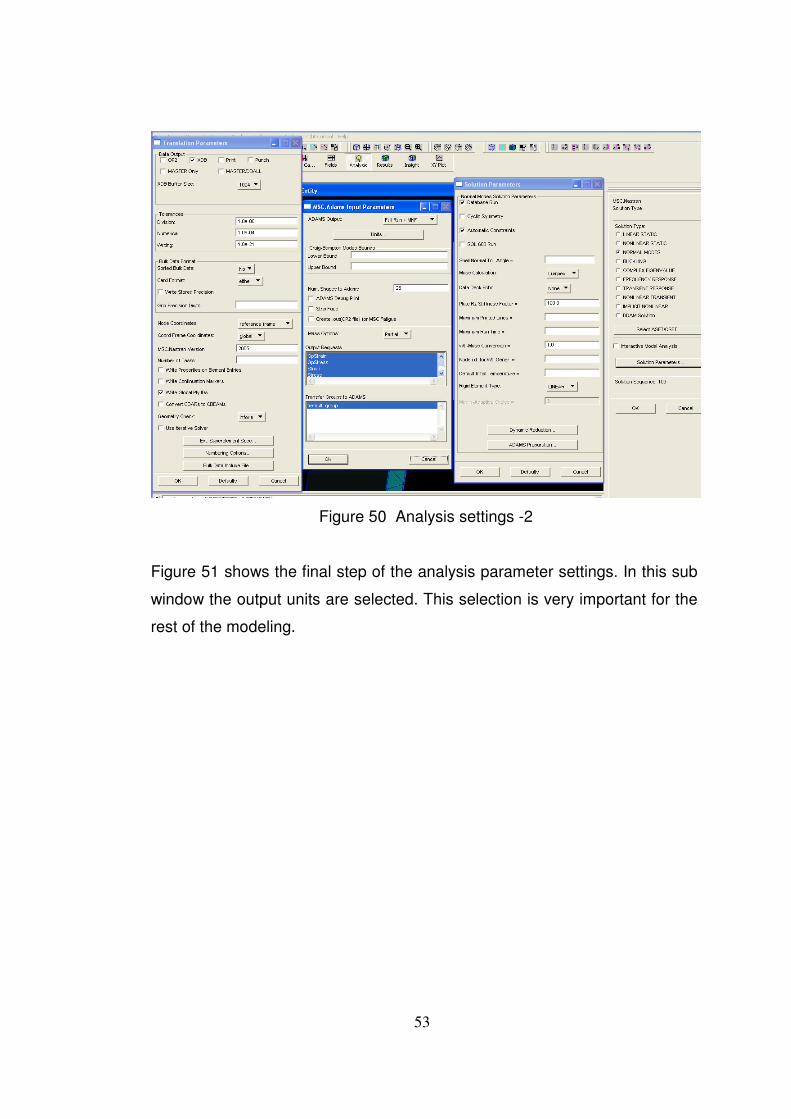
53
Figure 50 Analysis settings -2
Figure 51 shows the final step of the analysis parameter settings. In this sub
window the output units are selected. This selection is very important for the
rest of the modeling.
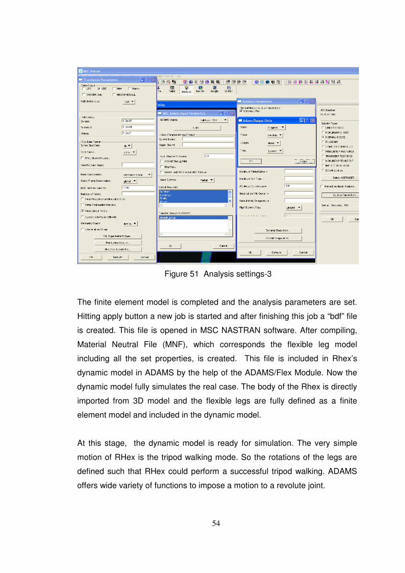
54
Figure 51 Analysis settings-3
The finite element model is completed and the analysis parameters are set.
Hitting apply button a new job is started and after finishing this job a “bdf” file
is created. This file is opened in MSC NASTRAN software. After compiling,
Material Neutral File (MNF), which corresponds the flexible leg model
including all the set properties, is created. This file is included in Rhex’s
dynamic model in ADAMS by the help of the ADAMS/Flex Module. Now the
dynamic model fully simulates the real case. The body of the Rhex is directly
imported from 3D model and the flexible legs are fully defined as a finite
element model and included in the dynamic model.
At this stage, the dynamic model is ready for simulation. The very simple
motion of RHex is the tripod walking mode. So the rotations of the legs are
defined such that RHex could perform a successful tripod walking. ADAMS
offers wide variety of functions to impose a motion to a revolute joint.
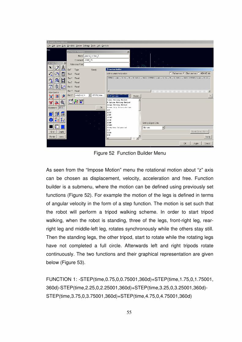
55
Figure 52 Function Builder Menu
As seen from the “Impose Motion” menu the rotational motion about “z” axis
can be chosen as displacement, velocity, acceleration and free. Function
builder is a submenu, where the motion can be defined using previously set
functions (Figure 52). For example the motion of the legs is defined in terms
of angular velocity in the form of a step function. The motion is set such that
the robot will perform a tripod walking scheme. In order to start tripod
walking, when the robot is standing, three of the legs, front-right leg, rear-
right leg and middle-left leg, rotates synchronously while the others stay still.
Then the standing legs, the other tripod, start to rotate while the rotating legs
have not completed a full circle. Afterwards left and right tripods rotate
continuously. The two functions and their graphical representation are given
below (Figure 53).
FUNCTION 1: -STEP(time,0.75,0,0.75001,360d)+STEP(time,1.75,0,1.75001,
360d)-STEP(time,2.25,0,2.25001,360d)+STEP(time,3.25,0,3.25001,360d)-
STEP(time,3.75,0,3.75001,360d)+STEP(time,4.75,0,4.75001,360d)
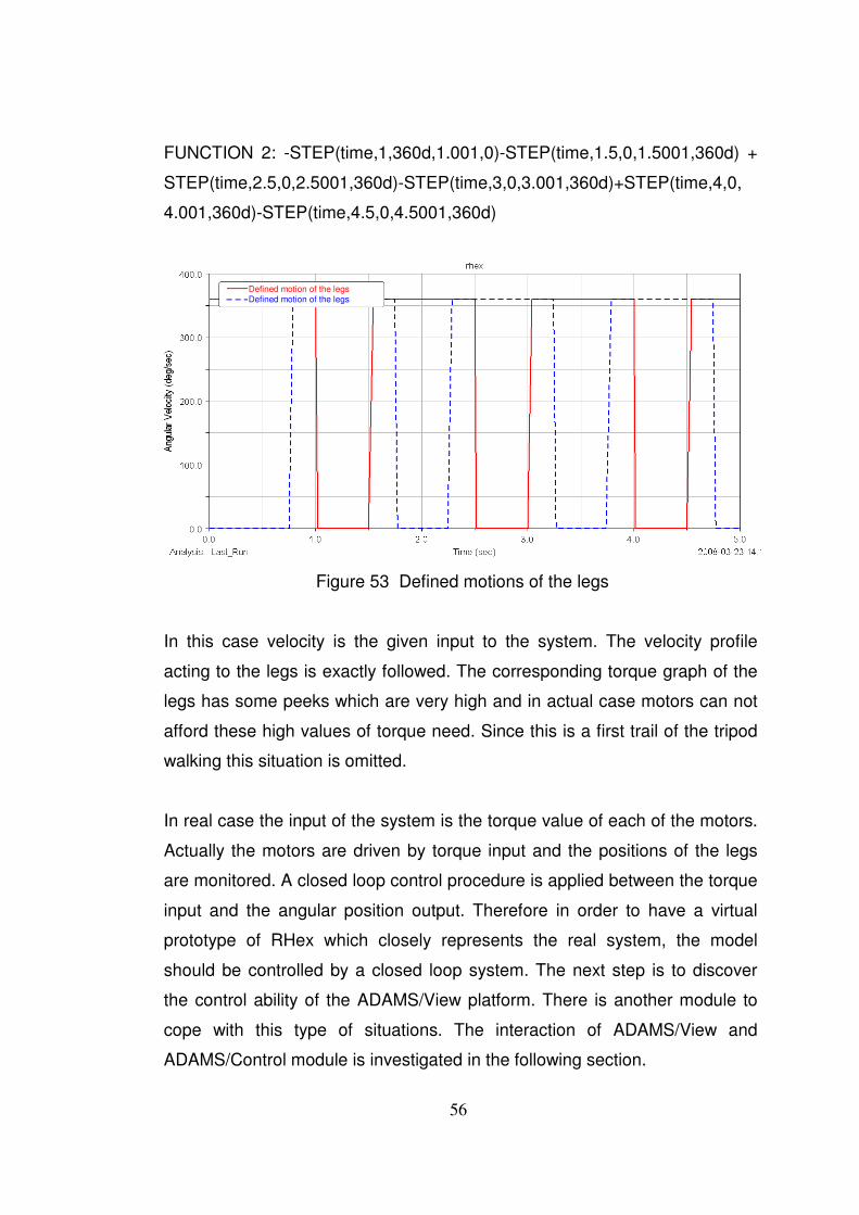
56
FUNCTION 2: -STEP(time,1,360d,1.001,0)-STEP(time,1.5,0,1.5001,360d) +
STEP(time,2.5,0,2.5001,360d)-STEP(time,3,0,3.001,360d)+STEP(time,4,0,
4.001,360d)-STEP(time,4.5,0,4.5001,360d)
Figure 53 Defined motions of the legs
In this case velocity is the given input to the system. The velocity profile
acting to the legs is exactly followed. The corresponding torque graph of the
legs has some peeks which are very high and in actual case motors can not
afford these high values of torque need. Since this is a first trail of the tripod
walking this situation is omitted.
In real case the input of the system is the torque value of each of the motors.
Actually the motors are driven by torque input and the positions of the legs
are monitored. A closed loop control procedure is applied between the torque
input and the angular position output. Therefore in order to have a virtual
prototype of RHex which closely represents the real system, the model
should be controlled by a closed loop system. The next step is to discover
the control ability of the ADAMS/View platform. There is another module to
cope with this type of situations. The interaction of ADAMS/View and
ADAMS/Control module is investigated in the following section.
Defined motion of the legs Defined motion of the legs
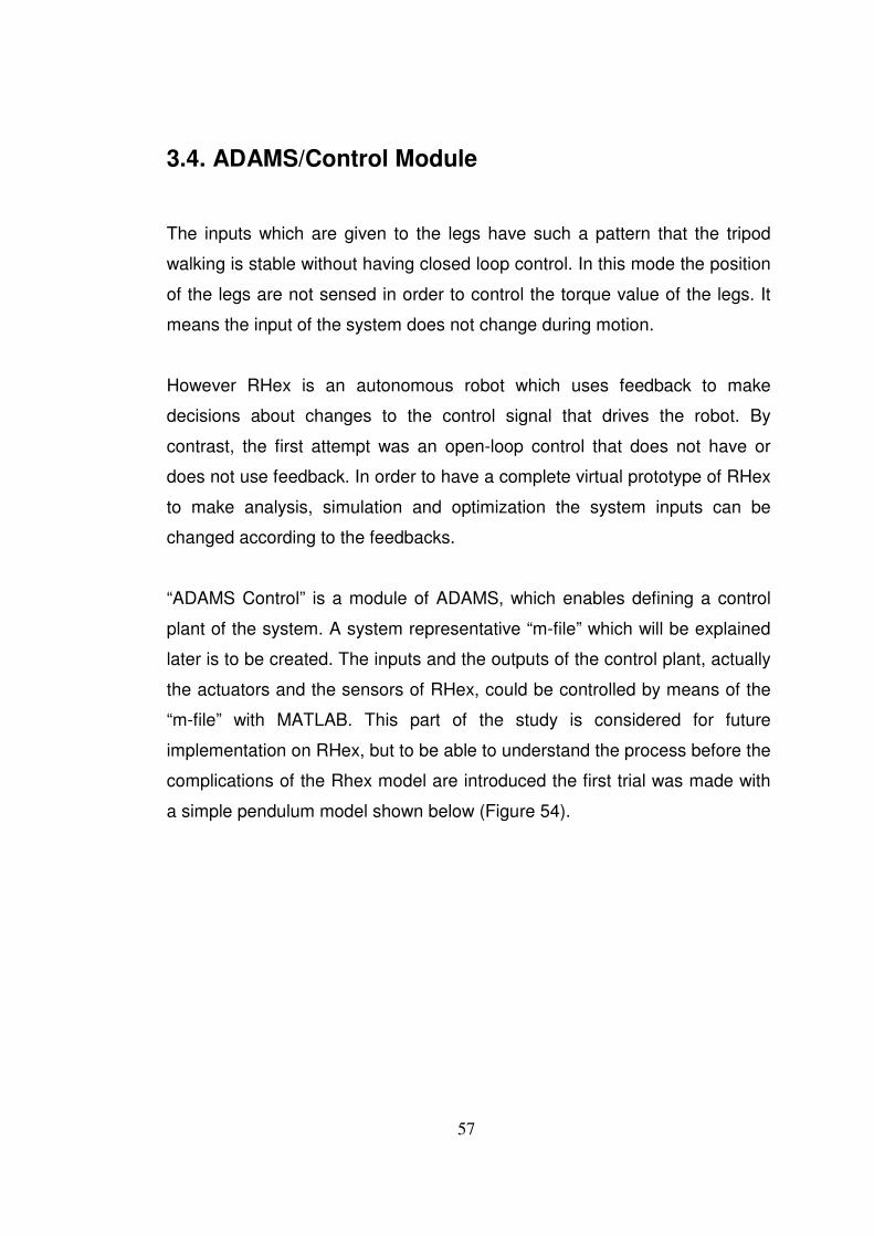
57
3.4. ADAMS/Control Module
The inputs which are given to the legs have such a pattern that the tripod
walking is stable without having closed loop control. In this mode the position
of the legs are not sensed in order to control the torque value of the legs. It
means the input of the system does not change during motion.
However RHex is an autonomous robot which uses feedback to make
decisions about changes to the control signal that drives the robot. By
contrast, the first attempt was an open-loop control that does not have or
does not use feedback. In order to have a complete virtual prototype of RHex
to make analysis, simulation and optimization the system inputs can be
changed according to the feedbacks.
“ADAMS Control” is a module of ADAMS, which enables defining a control
plant of the system. A system representative “m-file” which will be explained
later is to be created. The inputs and the outputs of the control plant, actually
the actuators and the sensors of RHex, could be controlled by means of the
“m-file” with MATLAB. This part of the study is considered for future
implementation on RHex, but to be able to understand the process before the
complications of the Rhex model are introduced the first trial was made with
a simple pendulum model shown below (Figure 54).
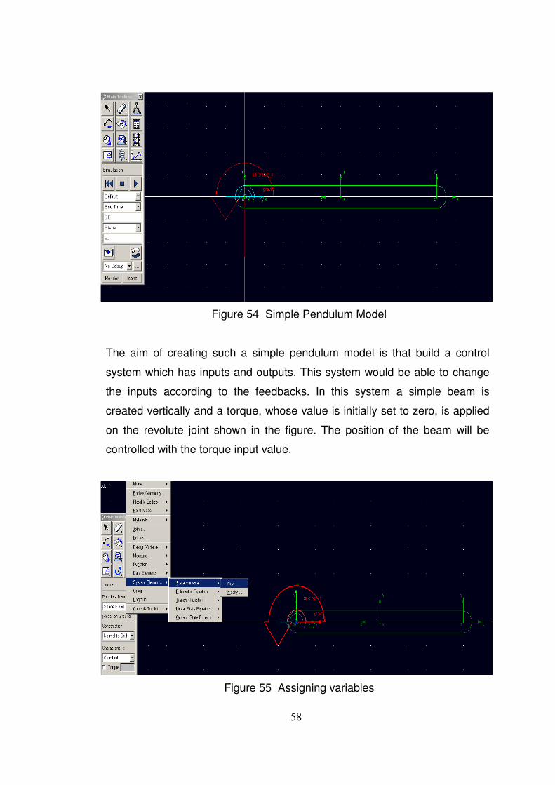
58
Figure 54 Simple Pendulum Model
The aim of creating such a simple pendulum model is that build a control
system which has inputs and outputs. This system would be able to change
the inputs according to the feedbacks. In this system a simple beam is
created vertically and a torque, whose value is initially set to zero, is applied
on the revolute joint shown in the figure. The position of the beam will be
controlled with the torque input value.
Figure 55 Assigning variables
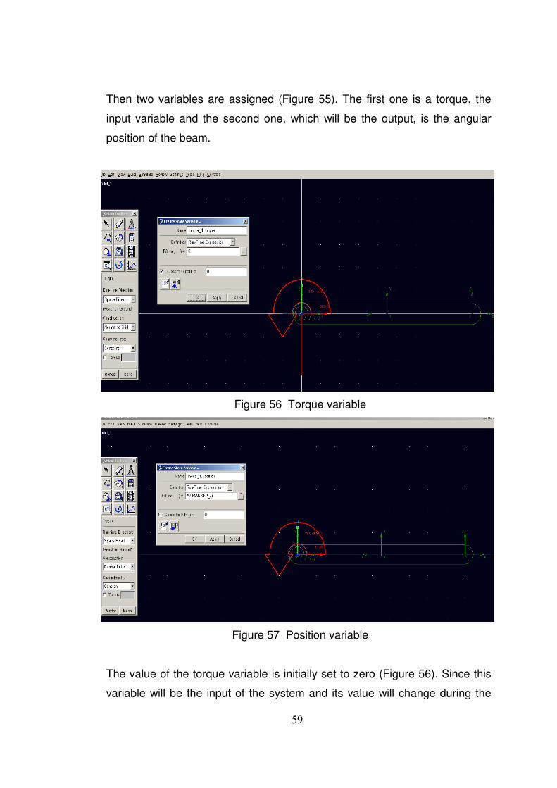
59
Then two variables are assigned (Figure 55). The first one is a torque, the
input variable and the second one, which will be the output, is the angular
position of the beam.
Figure 56 Torque variable
Figure 57 Position variable
The value of the torque variable is initially set to zero (Figure 56). Since this
variable will be the input of the system and its value will change during the
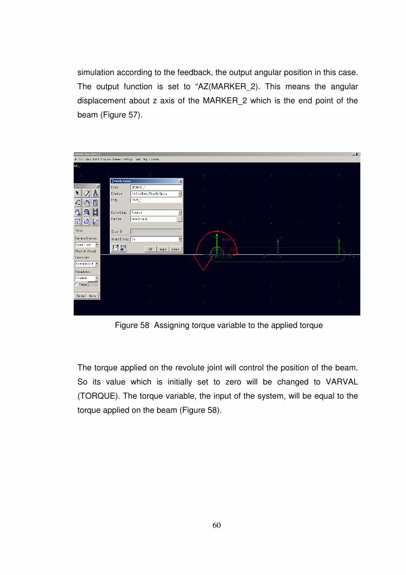
60
simulation according to the feedback, the output angular position in this case.
The output function is set to “AZ(MARKER_2). This means the angular
displacement about z axis of the MARKER_2 which is the end point of the
beam (Figure 57).
Figure 58 Assigning torque variable to the applied torque
The torque applied on the revolute joint will control the position of the beam.
So its value which is initially set to zero will be changed to VARVAL
(TORQUE). The torque variable, the input of the system, will be equal to the
torque applied on the beam (Figure 58).
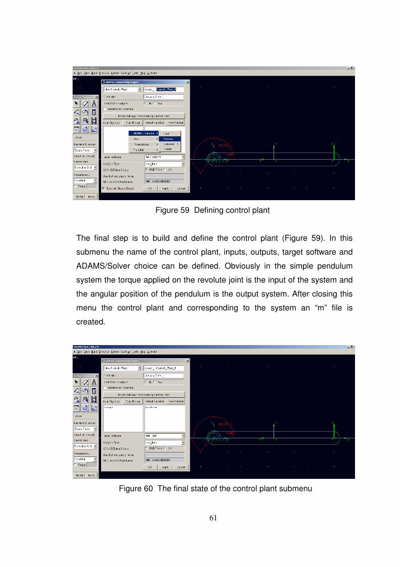
61
Figure 59 Defining control plant
The final step is to build and define the control plant (Figure 59). In this
submenu the name of the control plant, inputs, outputs, target software and
ADAMS/Solver choice can be defined. Obviously in the simple pendulum
system the torque applied on the revolute joint is the input of the system and
the angular position of the pendulum is the output system. After closing this
menu the control plant and corresponding to the system an “m” file is
created.
Figure 60 The final state of the control plant submenu
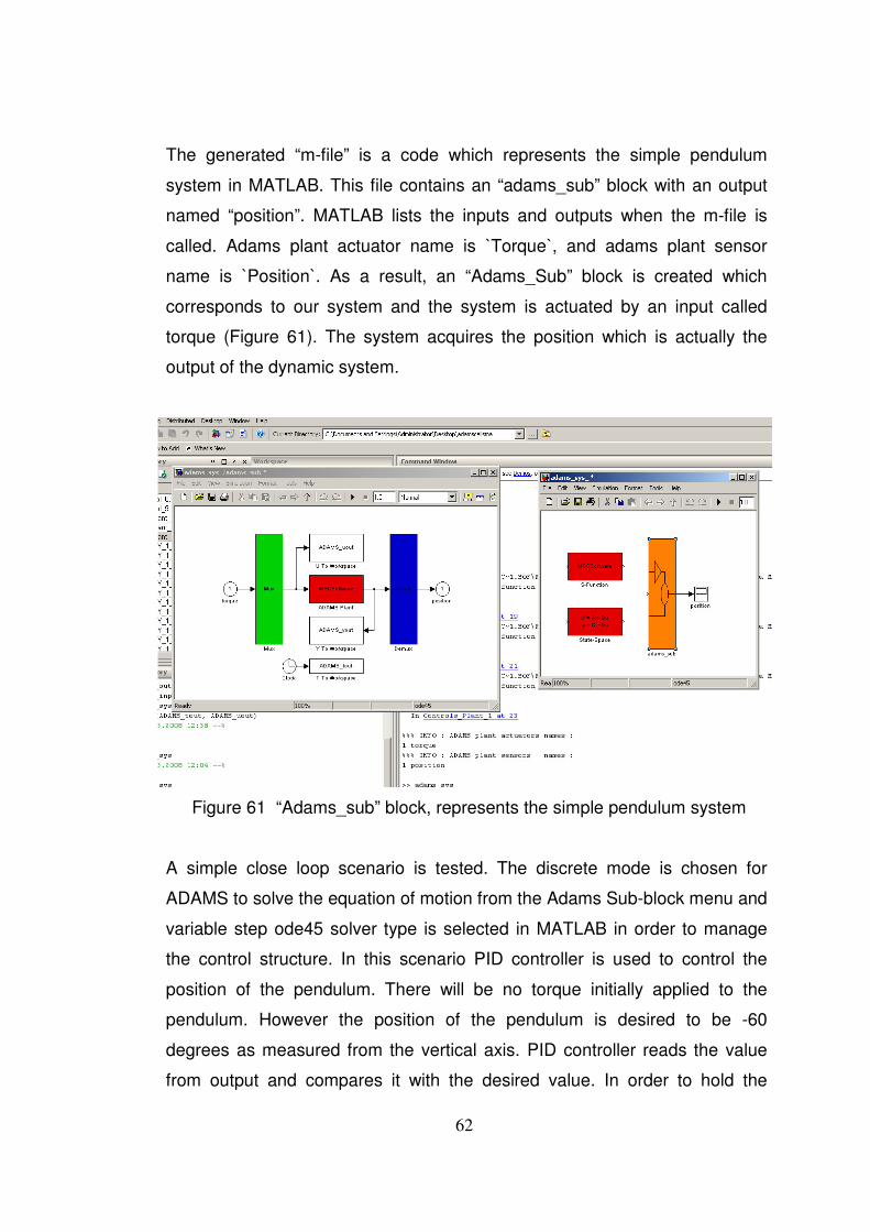
62
The generated “m-file” is a code which represents the simple pendulum
system in MATLAB. This file contains an “adams_sub” block with an output
named “position”. MATLAB lists the inputs and outputs when the m-file is
called. Adams plant actuator name is `Torque`, and adams plant sensor
name is `Position`. As a result, an “Adams_Sub” block is created which
corresponds to our system and the system is actuated by an input called
torque (Figure 61). The system acquires the position which is actually the
output of the dynamic system.
Figure 61 “Adams_sub” block, represents the simple pendulum system
A simple close loop scenario is tested. The discrete mode is chosen for
ADAMS to solve the equation of motion from the Adams Sub-block menu and
variable step ode45 solver type is selected in MATLAB in order to manage
the control structure. In this scenario PID controller is used to control the
position of the pendulum. There will be no torque initially applied to the
pendulum. However the position of the pendulum is desired to be -60
degrees as measured from the vertical axis. PID controller reads the value
from output and compares it with the desired value. In order to hold the
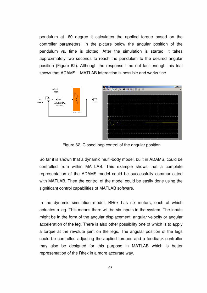
63
pendulum at -60 degree it calculates the applied torque based on the
controller parameters. In the picture below the angular position of the
pendulum vs. time is plotted. After the simulation is started, it takes
approximately two seconds to reach the pendulum to the desired angular
position (Figure 62). Although the response time not fast enough this trial
shows that ADAMS – MATLAB interaction is possible and works fine.
Figure 62 Closed loop control of the angular position
So far it is shown that a dynamic multi-body model, built in ADAMS, could be
controlled from within MATLAB. This example shows that a complete
representation of the ADAMS model could be successfully communicated
with MATLAB. Then the control of the model could be easily done using the
significant control capabilities of MATLAB software.
In the dynamic simulation model, RHex has six motors, each of which
actuates a leg. This means there will be six inputs in the system. The inputs
might be in the form of the angular displacement, angular velocity or angular
acceleration of the leg. There is also other possibility one of which is to apply
a torque at the revolute joint on the legs. The angular position of the legs
could be controlled adjusting the applied torques and a feedback controller
may also be designed for this purpose in MATLAB which is better
representation of the Rhex in a more accurate way.
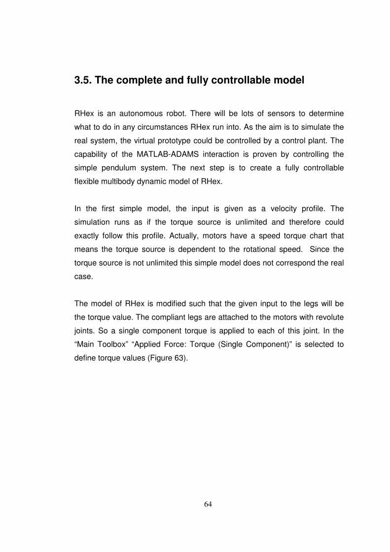
64
3.5. The complete and fully controllable model
RHex is an autonomous robot. There will be lots of sensors to determine
what to do in any circumstances RHex run into. As the aim is to simulate the
real system, the virtual prototype could be controlled by a control plant. The
capability of the MATLAB-ADAMS interaction is proven by controlling the
simple pendulum system. The next step is to create a fully controllable
flexible multibody dynamic model of RHex.
In the first simple model, the input is given as a velocity profile. The
simulation runs as if the torque source is unlimited and therefore could
exactly follow this profile. Actually, motors have a speed torque chart that
means the torque source is dependent to the rotational speed. Since the
torque source is not unlimited this simple model does not correspond the real
case.
The model of RHex is modified such that the given input to the legs will be
the torque value. The compliant legs are attached to the motors with revolute
joints. So a single component torque is applied to each of this joint. In the
“Main Toolbox” “Applied Force: Torque (Single Component)” is selected to
define torque values (Figure 63).
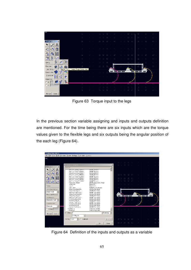
65
Figure 63 Torque input to the legs
In the previous section variable assigning and inputs and outputs definition
are mentioned. For the time being there are six inputs which are the torque
values given to the flexible legs and six outputs being the angular position of
the each leg (Figure 64).
Figure 64 Definition of the inputs and outputs as a variable
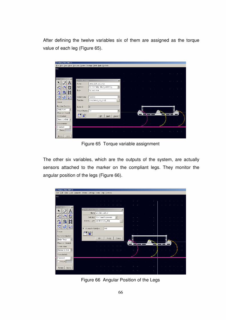
66
After defining the twelve variables six of them are assigned as the torque
value of each leg (Figure 65).
Figure 65 Torque variable assignment
The other six variables, which are the outputs of the system, are actually
sensors attached to the marker on the compliant legs. They monitor the
angular position of the legs (Figure 66).
Figure 66 Angular Position of the Legs
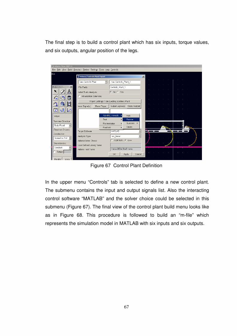
67
The final step is to build a control plant which has six inputs, torque values,
and six outputs, angular position of the legs.
Figure 67 Control Plant Definition
In the upper menu “Controls” tab is selected to define a new control plant.
The submenu contains the input and output signals list. Also the interacting
control software “MATLAB” and the solver choice could be selected in this
submenu (Figure 67). The final view of the control plant build menu looks like
as in Figure 68. This procedure is followed to build an “m-file” which
represents the simulation model in MATLAB with six inputs and six outputs.
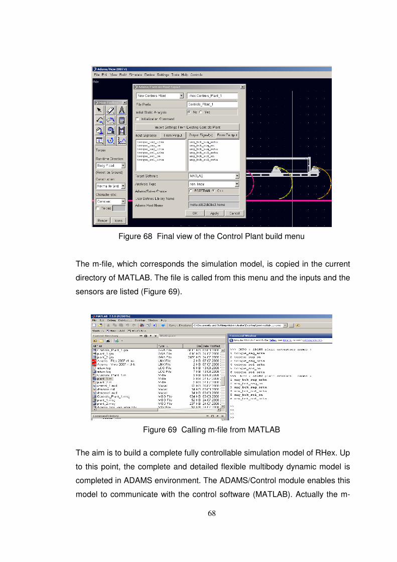
68
Figure 68 Final view of the Control Plant build menu
The m-file, which corresponds the simulation model, is copied in the current
directory of MATLAB. The file is called from this menu and the inputs and the
sensors are listed (Figure 69).
Figure 69 Calling m-file from MATLAB
The aim is to build a complete fully controllable simulation model of RHex. Up
to this point, the complete and detailed flexible multibody dynamic model is
completed in ADAMS environment. The ADAMS/Control module enables this
model to communicate with the control software (MATLAB). Actually the m-
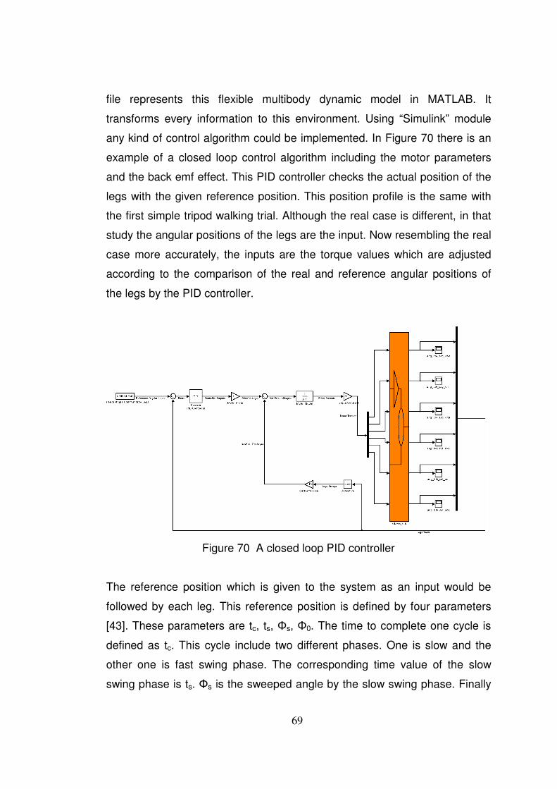
69
file represents this flexible multibody dynamic model in MATLAB. It
transforms every information to this environment. Using “Simulink” module
any kind of control algorithm could be implemented. In Figure 70 there is an
example of a closed loop control algorithm including the motor parameters
and the back emf effect. This PID controller checks the actual position of the
legs with the given reference position. This position profile is the same with
the first simple tripod walking trial. Although the real case is different, in that
study the angular positions of the legs are the input. Now resembling the real
case more accurately, the inputs are the torque values which are adjusted
according to the comparison of the real and reference angular positions of
the legs by the PID controller.
Figure 70 A closed loop PID controller
The reference position which is given to the system as an input would be
followed by each leg. This reference position is defined by four parameters
[43]. These parameters are tc, ts, Φs, Φ0. The time to complete one cycle is
defined as tc. This cycle include two different phases. One is slow and the
other one is fast swing phase. The corresponding time value of the slow
swing phase is ts. Φs is the sweeped angle by the slow swing phase. Finally
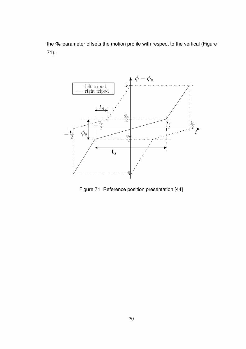
70
the Φ0 parameter offsets the motion profile with respect to the vertical (Figure
71).
Figure 71 Reference position presentation [44]
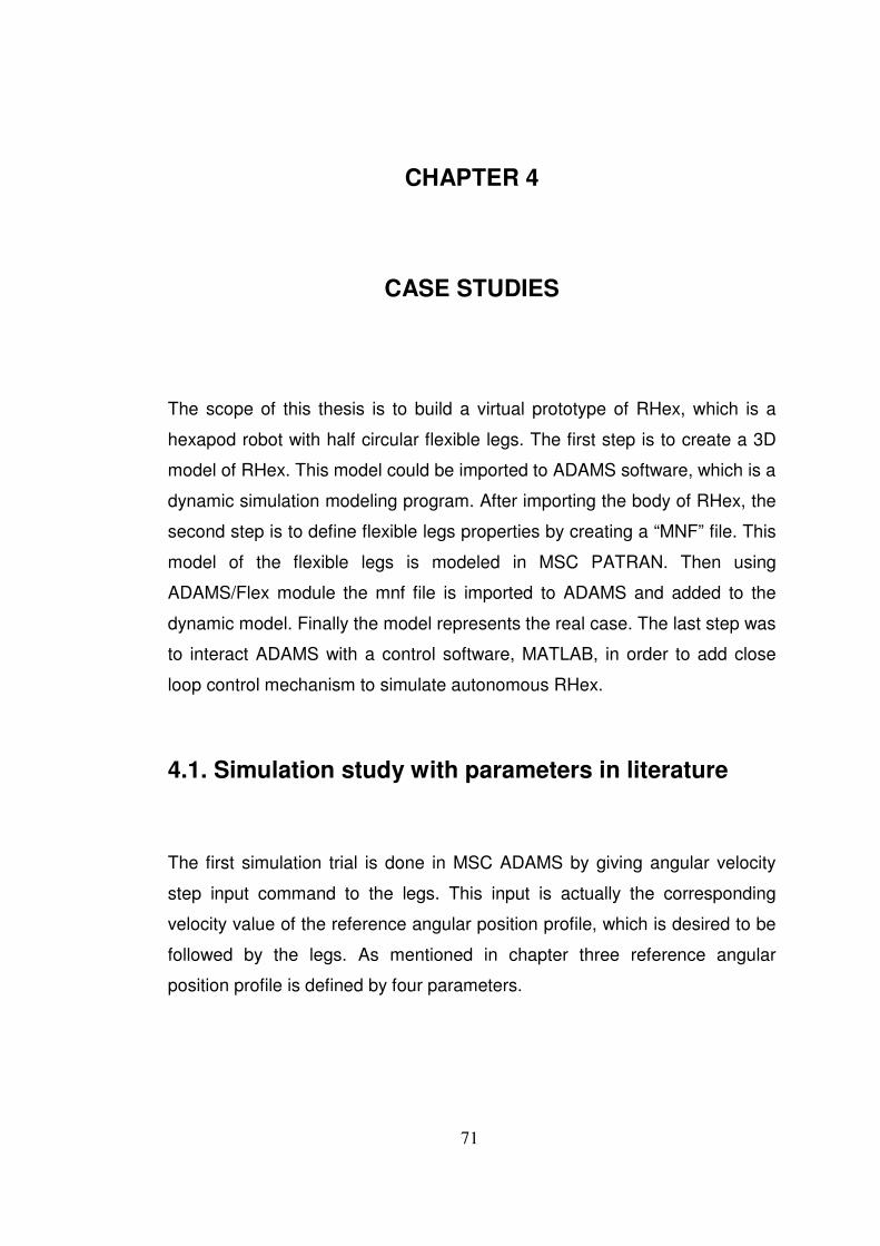
71
CHAPTER 4
CASE STUDIES
The scope of this thesis is to build a virtual prototype of RHex, which is a
hexapod robot with half circular flexible legs. The first step is to create a 3D
model of RHex. This model could be imported to ADAMS software, which is a
dynamic simulation modeling program. After importing the body of RHex, the
second step is to define flexible legs properties by creating a “MNF” file. This
model of the flexible legs is modeled in MSC PATRAN. Then using
ADAMS/Flex module the mnf file is imported to ADAMS and added to the
dynamic model. Finally the model represents the real case. The last step was
to interact ADAMS with a control software, MATLAB, in order to add close
loop control mechanism to simulate autonomous RHex.
4.1. Simulation study with parameters in literature
The first simulation trial is done in MSC ADAMS by giving angular velocity
step input command to the legs. This input is actually the corresponding
velocity value of the reference angular position profile, which is desired to be
followed by the legs. As mentioned in chapter three reference angular
position profile is defined by four parameters.
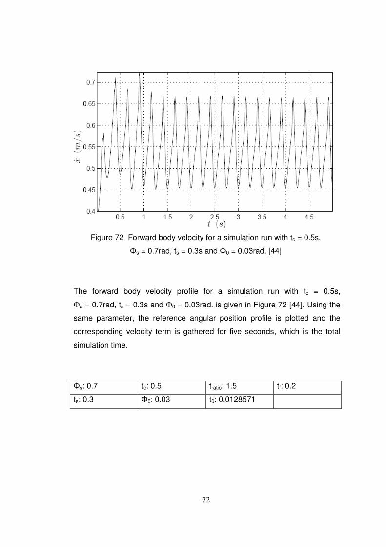
72
Figure 72 Forward body velocity for a simulation run with tc = 0.5s,
Φs = 0.7rad, ts = 0.3s and Φ0 = 0.03rad. [44]
The forward body velocity profile for a simulation run with tc = 0.5s,
Φs = 0.7rad, ts = 0.3s and Φ0 = 0.03rad. is given in Figure 72 [44]. Using the
same parameter, the reference angular position profile is plotted and the
corresponding velocity term is gathered for five seconds, which is the total
simulation time.
Φs: 0.7 tc: 0.5 tratio: 1.5 tf: 0.2
ts: 0.3 Φ0: 0.03 t0: 0.0128571
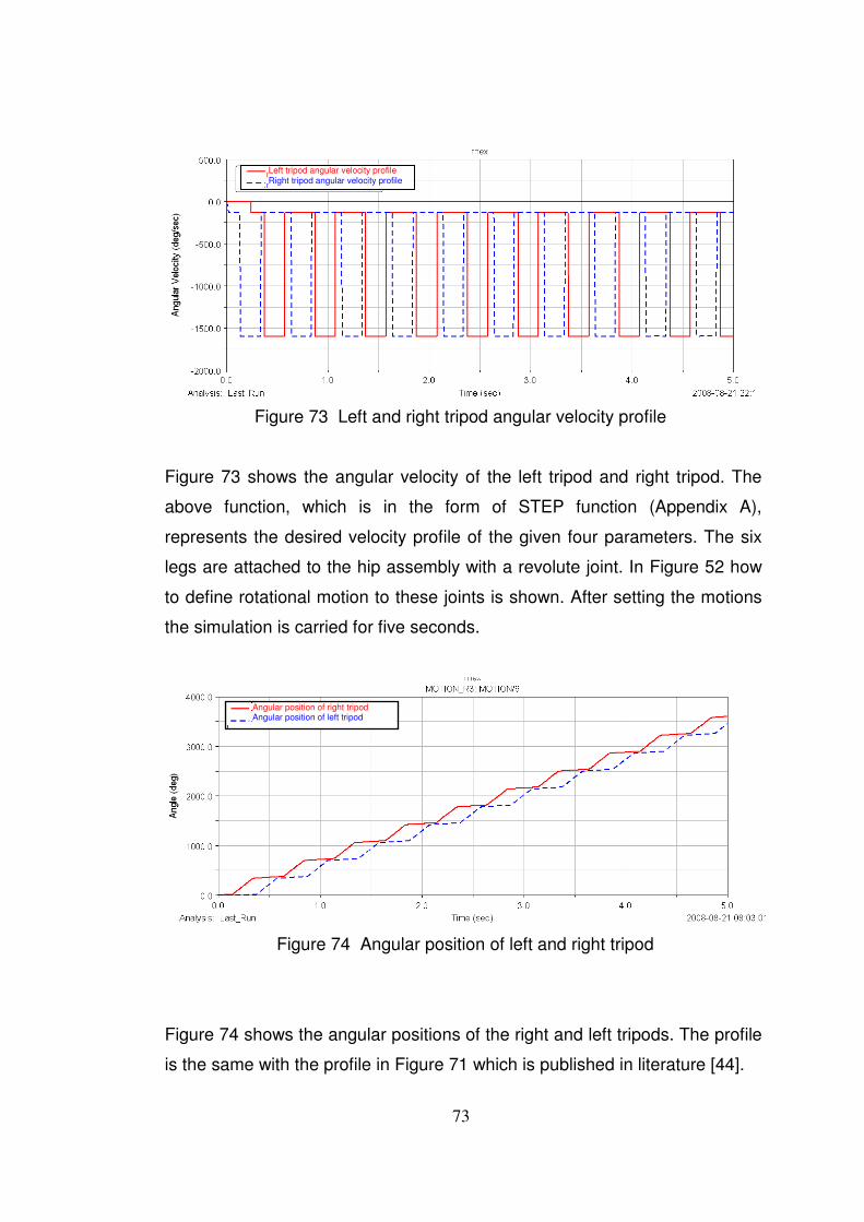
73
Figure 73 Left and right tripod angular velocity profile
Figure 73 shows the angular velocity of the left tripod and right tripod. The
above function, which is in the form of STEP function (Appendix A),
represents the desired velocity profile of the given four parameters. The six
legs are attached to the hip assembly with a revolute joint. In Figure 52 how
to define rotational motion to these joints is shown. After setting the motions
the simulation is carried for five seconds.
Figure 74 Angular position of left and right tripod
Figure 74 shows the angular positions of the right and left tripods. The profile
is the same with the profile in Figure 71 which is published in literature [44].
Left tripod angular velocity profile Right tripod angular velocity profile
Angular position of right tripod Angular position of left tripod
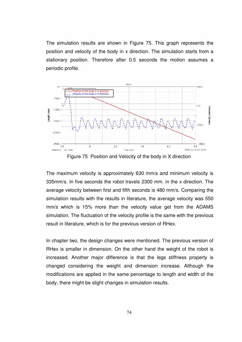
74
The simulation results are shown in Figure 75. This graph represents the
position and velocity of the body in x direction. The simulation starts from a
stationary position. Therefore after 0.5 seconds the motion assumes a
periodic profile.
Figure 75 Position and Velocity of the body in X direction
The maximum velocity is approximately 630 mm/s and minimum velocity is
335mm/s. In five seconds the robot travels 2300 mm. in the x direction. The
average velocity between first and fifth seconds is 480 mm/s. Comparing the
simulation results with the results in literature, the average velocity was 550
mm/s which is 15% more than the velocity value get from the ADAMS
simulation. The fluctuation of the velocity profile is the same with the previous
result in literature, which is for the previous version of RHex.
In chapter two, the design changes were mentioned. The previous version of
RHex is smaller in dimension. On the other hand the weight of the robot is
increased. Another major difference is that the legs stiffness property is
changed considering the weight and dimension increase. Although the
modifications are applied in the same percentage to length and width of the
body, there might be slight changes in simulation results.
Position of the body in X direction Velocity of the body in X direction
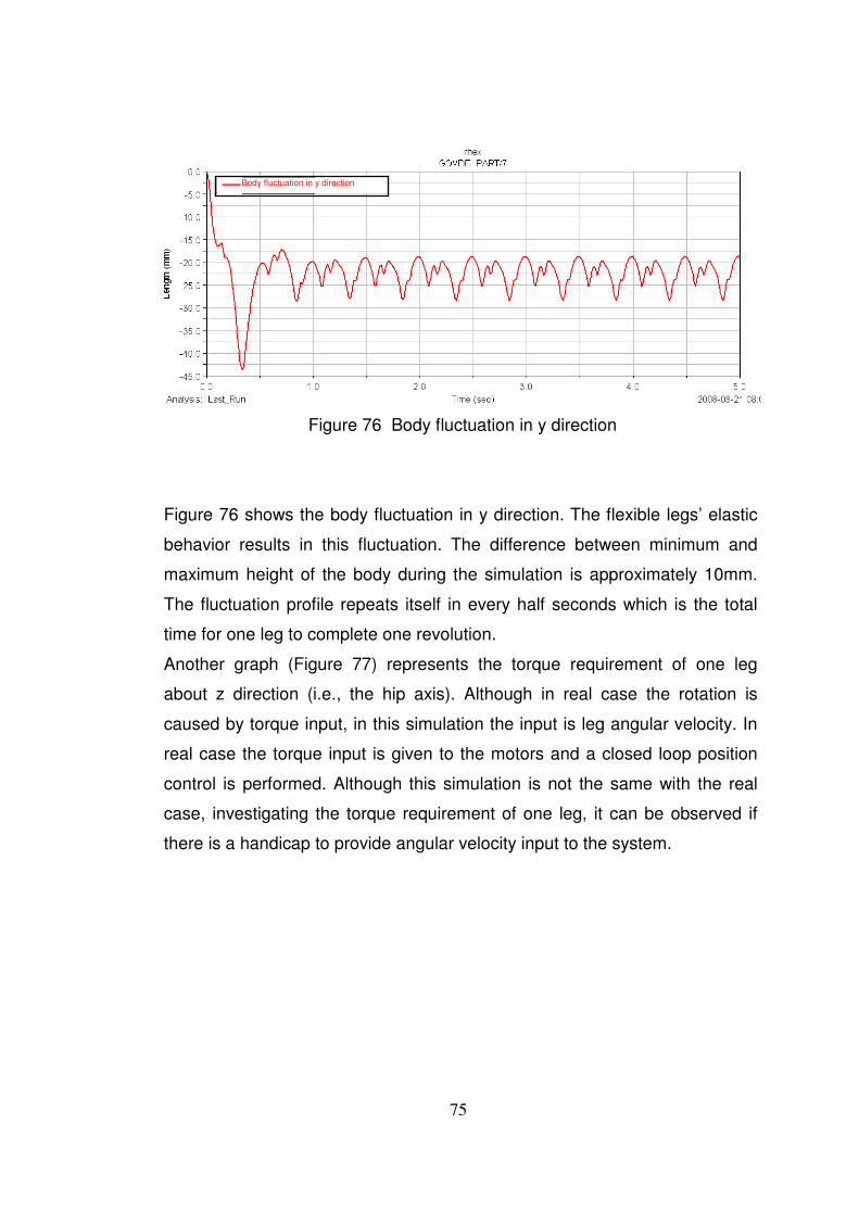
75
Figure 76 Body fluctuation in y direction
Figure 76 shows the body fluctuation in y direction. The flexible legs’ elastic
behavior results in this fluctuation. The difference between minimum and
maximum height of the body during the simulation is approximately 10mm.
The fluctuation profile repeats itself in every half seconds which is the total
time for one leg to complete one revolution.
Another graph (Figure 77) represents the torque requirement of one leg
about z direction (i.e., the hip axis). Although in real case the rotation is
caused by torque input, in this simulation the input is leg angular velocity. In
real case the torque input is given to the motors and a closed loop position
control is performed. Although this simulation is not the same with the real
case, investigating the torque requirement of one leg, it can be observed if
there is a handicap to provide angular velocity input to the system.
Body fluctuation in y direction
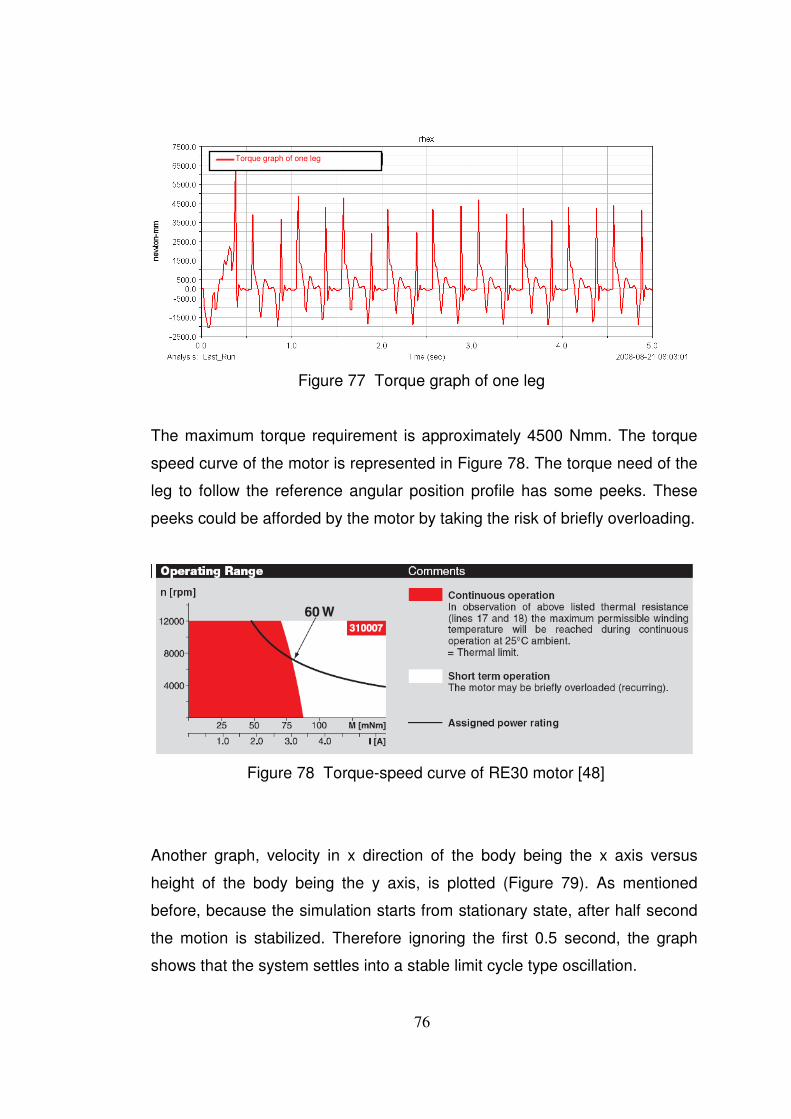
76
Figure 77 Torque graph of one leg
The maximum torque requirement is approximately 4500 Nmm. The torque
speed curve of the motor is represented in Figure 78. The torque need of the
leg to follow the reference angular position profile has some peeks. These
peeks could be afforded by the motor by taking the risk of briefly overloading.
Figure 78 Torque-speed curve of RE30 motor [48]
Another graph, velocity in x direction of the body being the x axis versus
height of the body being the y axis, is plotted (Figure 79). As mentioned
before, because the simulation starts from stationary state, after half second
the motion is stabilized. Therefore ignoring the first 0.5 second, the graph
shows that the system settles into a stable limit cycle type oscillation.
Torque graph of one leg
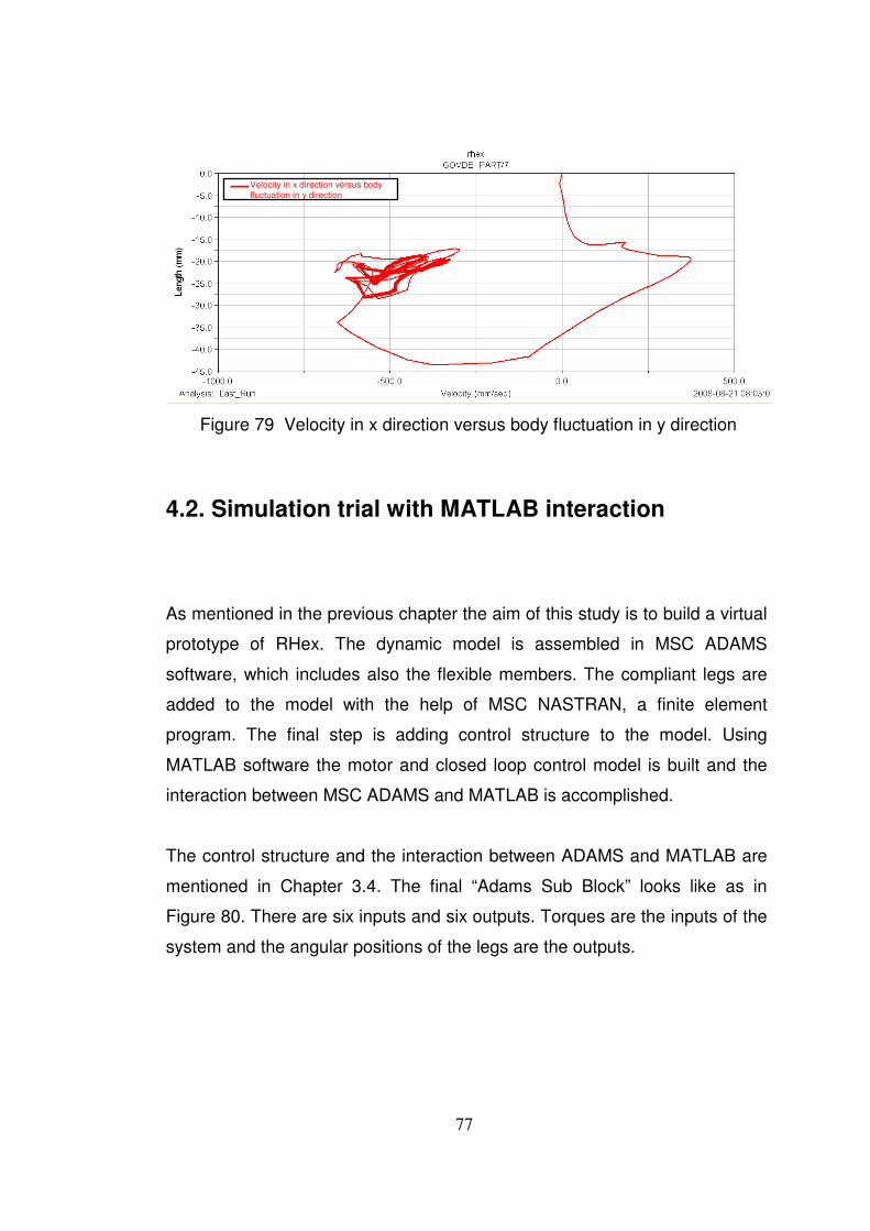
77
Figure 79 Velocity in x direction versus body fluctuation in y direction
4.2. Simulation trial with MATLAB interaction
As mentioned in the previous chapter the aim of this study is to build a virtual
prototype of RHex. The dynamic model is assembled in MSC ADAMS
software, which includes also the flexible members. The compliant legs are
added to the model with the help of MSC NASTRAN, a finite element
program. The final step is adding control structure to the model. Using
MATLAB software the motor and closed loop control model is built and the
interaction between MSC ADAMS and MATLAB is accomplished.
The control structure and the interaction between ADAMS and MATLAB are
mentioned in Chapter 3.4. The final “Adams Sub Block” looks like as in
Figure 80. There are six inputs and six outputs. Torques are the inputs of the
system and the angular positions of the legs are the outputs.
Velocity in x direction versus body fluctuation in y direction
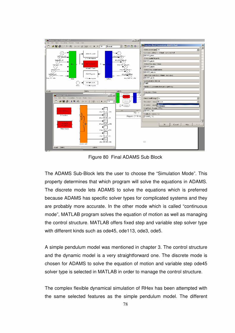
78
Figure 80 Final ADAMS Sub Block
The ADAMS Sub-Block lets the user to choose the “Simulation Mode”. This
property determines that which program will solve the equations in ADAMS.
The discrete mode lets ADAMS to solve the equations which is preferred
because ADAMS has specific solver types for complicated systems and they
are probably more accurate. In the other mode which is called “continuous
mode”, MATLAB program solves the equation of motion as well as managing
the control structure. MATLAB offers fixed step and variable step solver type
with different kinds such as ode45, ode113, ode3, ode5.
A simple pendulum model was mentioned in chapter 3. The control structure
and the dynamic model is a very straightforward one. The discrete mode is
chosen for ADAMS to solve the equation of motion and variable step ode45
solver type is selected in MATLAB in order to manage the control structure.
The complex flexible dynamical simulation of RHex has been attempted with
the same selected features as the simple pendulum model. The different
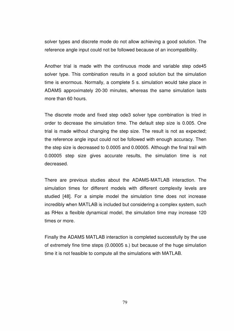
79
solver types and discrete mode do not allow achieving a good solution. The
reference angle input could not be followed because of an incompatibility.
Another trial is made with the continuous mode and variable step ode45
solver type. This combination results in a good solution but the simulation
time is enormous. Normally, a complete 5 s. simulation would take place in
ADAMS approximately 20-30 minutes, whereas the same simulation lasts
more than 60 hours.
The discrete mode and fixed step ode3 solver type combination is tried in
order to decrease the simulation time. The default step size is 0.005. One
trial is made without changing the step size. The result is not as expected;
the reference angle input could not be followed with enough accuracy. Then
the step size is decreased to 0.0005 and 0.00005. Although the final trail with
0.00005 step size gives accurate results, the simulation time is not
decreased.
There are previous studies about the ADAMS-MATLAB interaction. The
simulation times for different models with different complexity levels are
studied [48]. For a simple model the simulation time does not increase
incredibly when MATLAB is included but considering a complex system, such
as RHex a flexible dynamical model, the simulation time may increase 120
times or more.
Finally the ADAMS MATLAB interaction is completed successfully by the use
of extremely fine time steps (0.00005 s.) but because of the huge simulation
time it is not feasible to compute all the simulations with MATLAB.
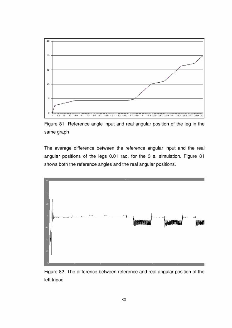
80
Figure 81 Reference angle input and real angular position of the leg in the
same graph
The average difference between the reference angular input and the real
angular positions of the legs 0.01 rad. for the 3 s. simulation. Figure 81
shows both the reference angles and the real angular positions.
Figure 82 The difference between reference and real angular position of the
left tripod
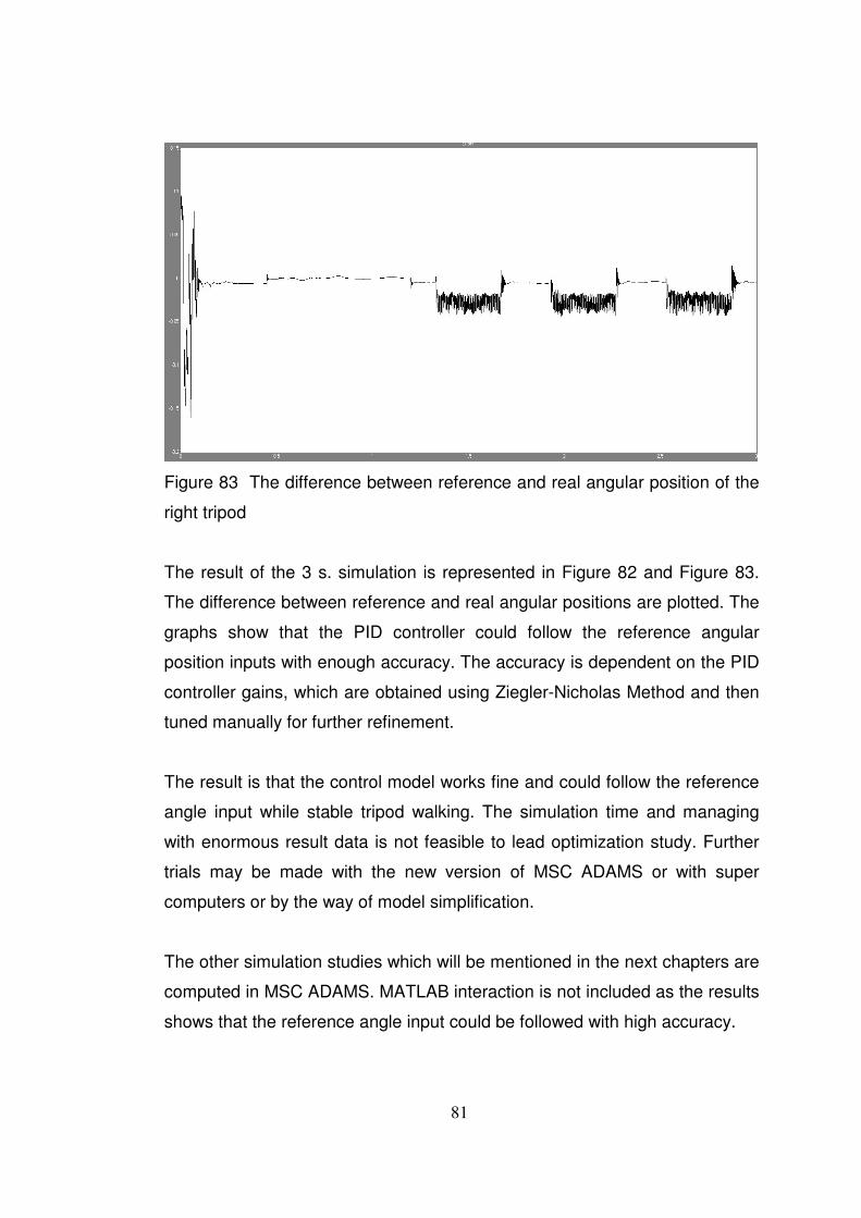
81
Figure 83 The difference between reference and real angular position of the
right tripod
The result of the 3 s. simulation is represented in Figure 82 and Figure 83.
The difference between reference and real angular positions are plotted. The
graphs show that the PID controller could follow the reference angular
position inputs with enough accuracy. The accuracy is dependent on the PID
controller gains, which are obtained using Ziegler-Nicholas Method and then
tuned manually for further refinement.
The result is that the control model works fine and could follow the reference
angle input while stable tripod walking. The simulation time and managing
with enormous result data is not feasible to lead optimization study. Further
trials may be made with the new version of MSC ADAMS or with super
computers or by the way of model simplification.
The other simulation studies which will be mentioned in the next chapters are
computed in MSC ADAMS. MATLAB interaction is not included as the results
shows that the reference angle input could be followed with high accuracy.
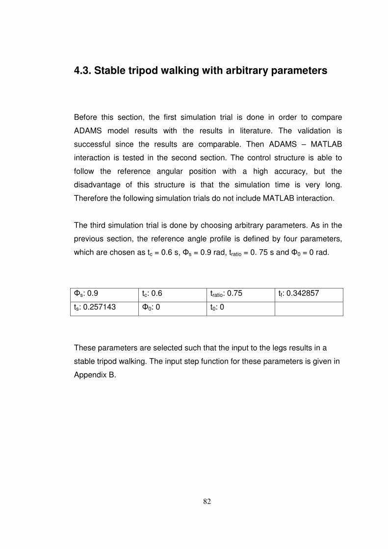
82
4.3. Stable tripod walking with arbitrary parameters
Before this section, the first simulation trial is done in order to compare
ADAMS model results with the results in literature. The validation is
successful since the results are comparable. Then ADAMS – MATLAB
interaction is tested in the second section. The control structure is able to
follow the reference angular position with a high accuracy, but the
disadvantage of this structure is that the simulation time is very long.
Therefore the following simulation trials do not include MATLAB interaction.
The third simulation trial is done by choosing arbitrary parameters. As in the
previous section, the reference angle profile is defined by four parameters,
which are chosen as tc = 0.6 s, Φs = 0.9 rad, tratio = 0. 75 s and Φ0 = 0 rad.
Φs: 0.9 tc: 0.6 tratio: 0.75 tf: 0.342857
ts: 0.257143 Φ0: 0 t0: 0
These parameters are selected such that the input to the legs results in a
stable tripod walking. The input step function for these parameters is given in
Appendix B.
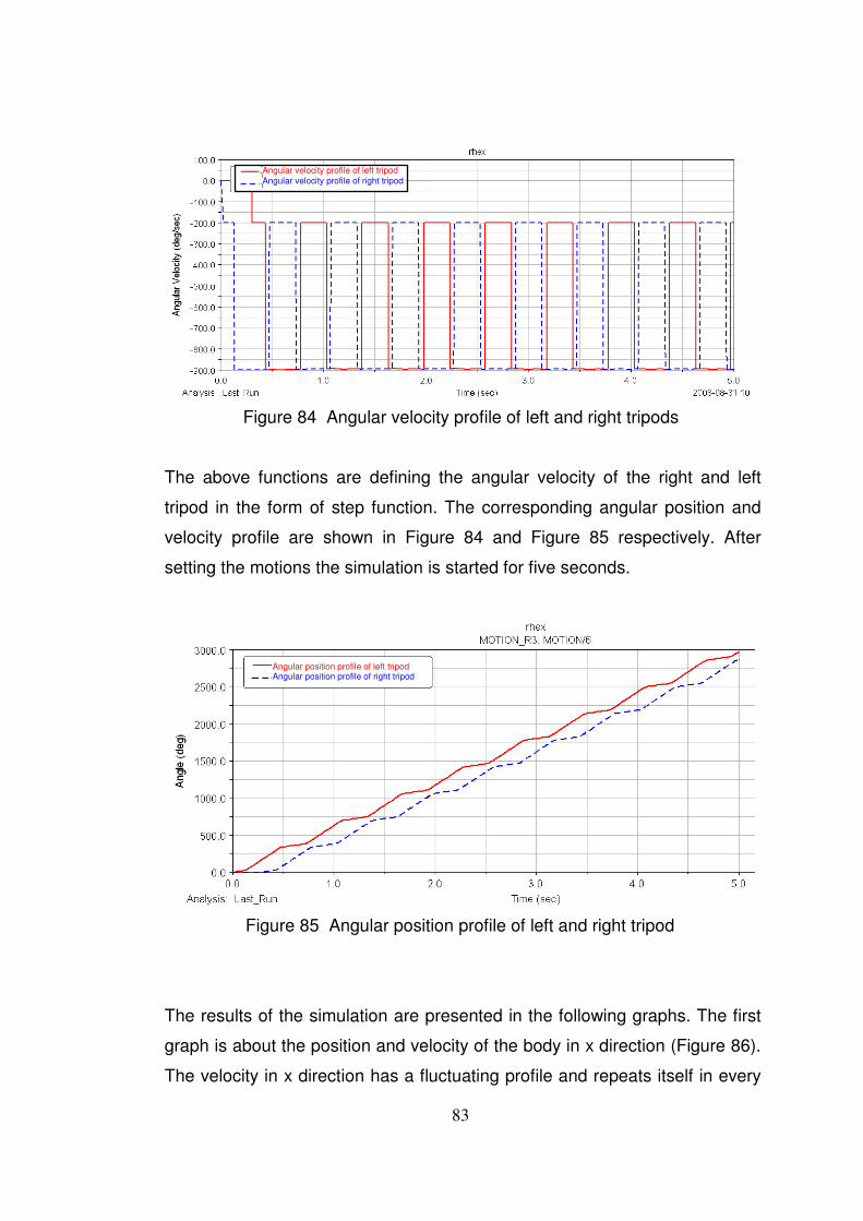
83
Figure 84 Angular velocity profile of left and right tripods
The above functions are defining the angular velocity of the right and left
tripod in the form of step function. The corresponding angular position and
velocity profile are shown in Figure 84 and Figure 85 respectively. After
setting the motions the simulation is started for five seconds.
Figure 85 Angular position profile of left and right tripod
The results of the simulation are presented in the following graphs. The first
graph is about the position and velocity of the body in x direction (Figure 86).
The velocity in x direction has a fluctuating profile and repeats itself in every
Angular velocity profile of left tripod Angular velocity profile of right tripod
Angular position profile of left tripod Angular position profile of right tripod
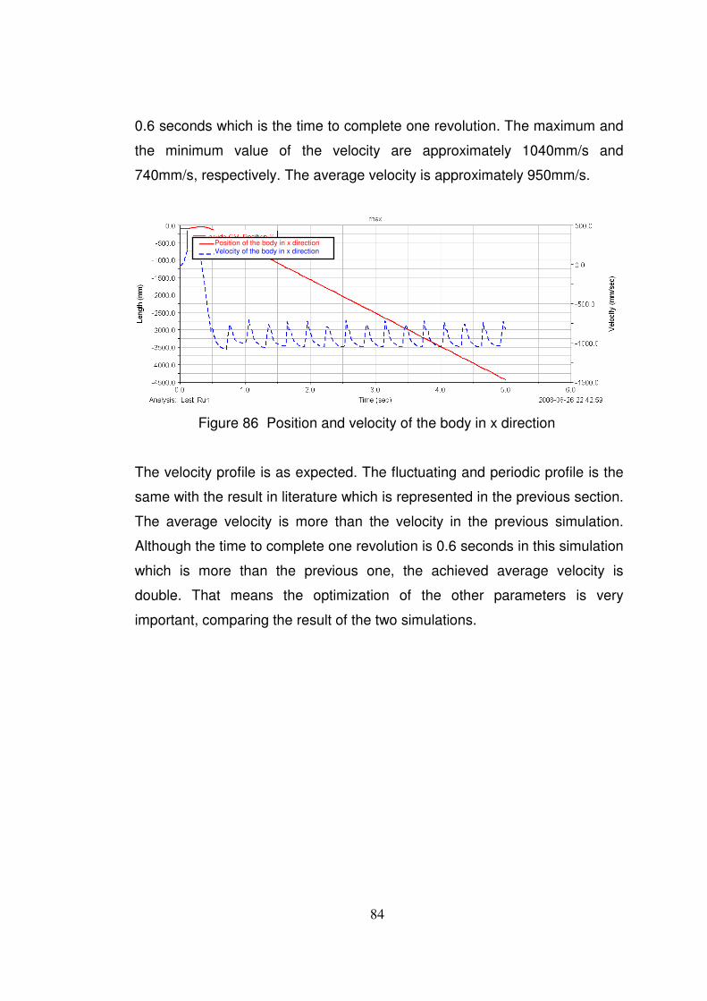
84
0.6 seconds which is the time to complete one revolution. The maximum and
the minimum value of the velocity are approximately 1040mm/s and
740mm/s, respectively. The average velocity is approximately 950mm/s.
Figure 86 Position and velocity of the body in x direction
The velocity profile is as expected. The fluctuating and periodic profile is the
same with the result in literature which is represented in the previous section.
The average velocity is more than the velocity in the previous simulation.
Although the time to complete one revolution is 0.6 seconds in this simulation
which is more than the previous one, the achieved average velocity is
double. That means the optimization of the other parameters is very
important, comparing the result of the two simulations.
Position of the body in x direction Velocity of the body in x direction
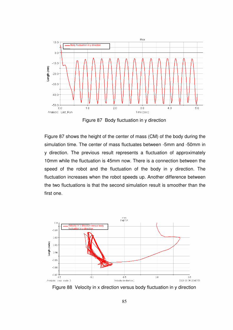
85
Figure 87 Body fluctuation in y direction
Figure 87 shows the height of the center of mass (CM) of the body during the
simulation time. The center of mass fluctuates between -5mm and -50mm in
y direction. The previous result represents a fluctuation of approximately
10mm while the fluctuation is 45mm now. There is a connection between the
speed of the robot and the fluctuation of the body in y direction. The
fluctuation increases when the robot speeds up. Another difference between
the two fluctuations is that the second simulation result is smoother than the
first one.
Figure 88 Velocity in x direction versus body fluctuation in y direction
Body fluctuation in y direction
Velocity in x direction versus body fluctuation in y direction
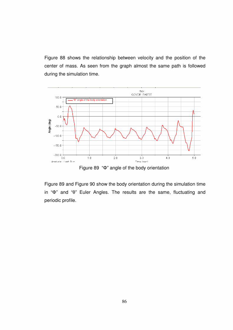
86
Figure 88 shows the relationship between velocity and the position of the
center of mass. As seen from the graph almost the same path is followed
during the simulation time.
Figure 89 “Φ” angle of the body orientation
Figure 89 and Figure 90 show the body orientation during the simulation time
in “Φ” and “θ” Euler Angles. The results are the same, fluctuating and
periodic profile.
“Φ” angle of the body orientation
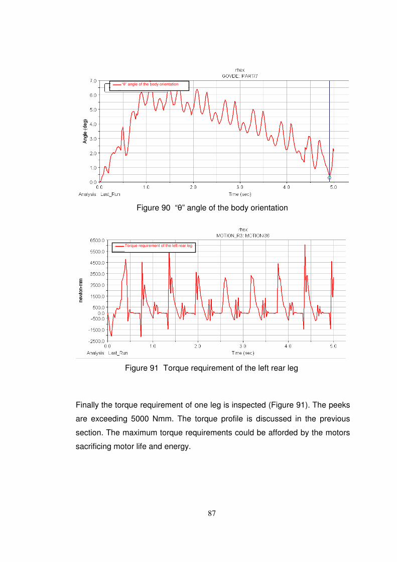
87
Figure 90 “θ” angle of the body orientation
Figure 91 Torque requirement of the left rear leg
Finally the torque requirement of one leg is inspected (Figure 91). The peeks
are exceeding 5000 Nmm. The torque profile is discussed in the previous
section. The maximum torque requirements could be afforded by the motors
sacrificing motor life and energy.
“θ” angle of the body orientation
Torque requirement of the left rear leg
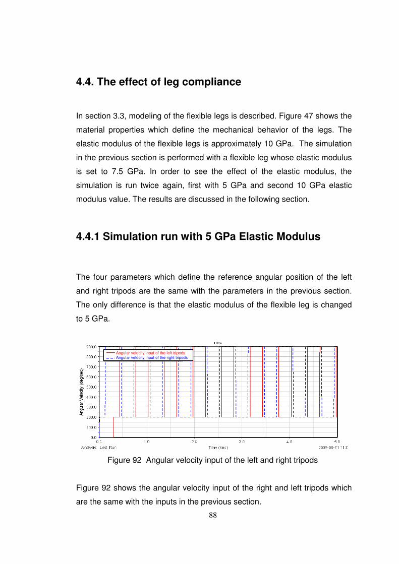
88
4.4. The effect of leg compliance
In section 3.3, modeling of the flexible legs is described. Figure 47 shows the
material properties which define the mechanical behavior of the legs. The
elastic modulus of the flexible legs is approximately 10 GPa. The simulation
in the previous section is performed with a flexible leg whose elastic modulus
is set to 7.5 GPa. In order to see the effect of the elastic modulus, the
simulation is run twice again, first with 5 GPa and second 10 GPa elastic
modulus value. The results are discussed in the following section.
4.4.1 Simulation run with 5 GPa Elastic Modulus
The four parameters which define the reference angular position of the left
and right tripods are the same with the parameters in the previous section.
The only difference is that the elastic modulus of the flexible leg is changed
to 5 GPa.
Figure 92 Angular velocity input of the left and right tripods
Figure 92 shows the angular velocity input of the right and left tripods which
are the same with the inputs in the previous section.
Angular velocity input of the left tripods Angular velocity input of the right tripods
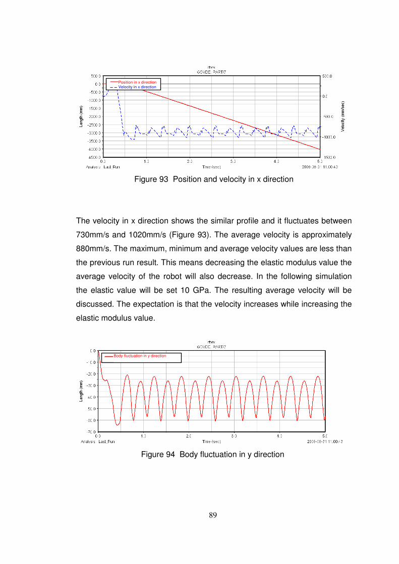
89
Figure 93 Position and velocity in x direction
The velocity in x direction shows the similar profile and it fluctuates between
730mm/s and 1020mm/s (Figure 93). The average velocity is approximately
880mm/s. The maximum, minimum and average velocity values are less than
the previous run result. This means decreasing the elastic modulus value the
average velocity of the robot will also decrease. In the following simulation
the elastic value will be set 10 GPa. The resulting average velocity will be
discussed. The expectation is that the velocity increases while increasing the
elastic modulus value.
Figure 94 Body fluctuation in y direction
Position in x direction Velocity in x direction
Body fluctuation in y direction
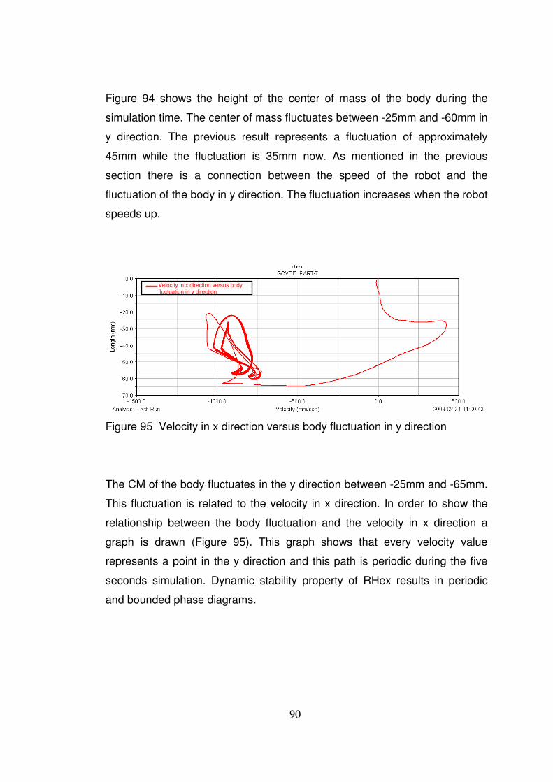
90
Figure 94 shows the height of the center of mass of the body during the
simulation time. The center of mass fluctuates between -25mm and -60mm in
y direction. The previous result represents a fluctuation of approximately
45mm while the fluctuation is 35mm now. As mentioned in the previous
section there is a connection between the speed of the robot and the
fluctuation of the body in y direction. The fluctuation increases when the robot
speeds up.
Figure 95 Velocity in x direction versus body fluctuation in y direction
The CM of the body fluctuates in the y direction between -25mm and -65mm.
This fluctuation is related to the velocity in x direction. In order to show the
relationship between the body fluctuation and the velocity in x direction a
graph is drawn (Figure 95). This graph shows that every velocity value
represents a point in the y direction and this path is periodic during the five
seconds simulation. Dynamic stability property of RHex results in periodic
and bounded phase diagrams.
Velocity in x direction versus body fluctuation in y direction
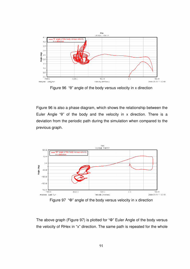
91
Figure 96 “θ” angle of the body versus velocity in x direction
Figure 96 is also a phase diagram, which shows the relationship between the
Euler Angle “θ” of the body and the velocity in x direction. There is a
deviation from the periodic path during the simulation when compared to the
previous graph.
Figure 97 “Φ” angle of the body versus velocity in x direction
The above graph (Figure 97) is plotted for “Φ” Euler Angle of the body versus
the velocity of RHex in “x” direction. The same path is repeated for the whole
“θ” angle of the body versus velocity in x direction
“Φ” angle of the body versus velocity in x direction
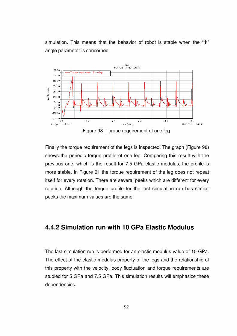
92
simulation. This means that the behavior of robot is stable when the “Φ”
angle parameter is concerned.
Figure 98 Torque requirement of one leg
Finally the torque requirement of the legs is inspected. The graph (Figure 98)
shows the periodic torque profile of one leg. Comparing this result with the
previous one, which is the result for 7.5 GPa elastic modulus, the profile is
more stable. In Figure 91 the torque requirement of the leg does not repeat
itself for every rotation. There are several peeks which are different for every
rotation. Although the torque profile for the last simulation run has similar
peeks the maximum values are the same.
4.4.2 Simulation run with 10 GPa Elastic Modulus
The last simulation run is performed for an elastic modulus value of 10 GPa.
The effect of the elastic modulus property of the legs and the relationship of
this property with the velocity, body fluctuation and torque requirements are
studied for 5 GPa and 7.5 GPa. This simulation results will emphasize these
dependencies.
Torque requirement of one leg
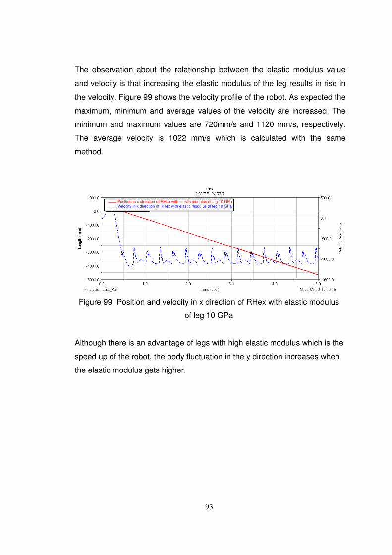
93
The observation about the relationship between the elastic modulus value
and velocity is that increasing the elastic modulus of the leg results in rise in
the velocity. Figure 99 shows the velocity profile of the robot. As expected the
maximum, minimum and average values of the velocity are increased. The
minimum and maximum values are 720mm/s and 1120 mm/s, respectively.
The average velocity is 1022 mm/s which is calculated with the same
method.
Figure 99 Position and velocity in x direction of RHex with elastic modulus
of leg 10 GPa
Although there is an advantage of legs with high elastic modulus which is the
speed up of the robot, the body fluctuation in the y direction increases when
the elastic modulus gets higher.
Position in x direction of RHex with elastic modulus of leg 10 GPa Velocity in x direction of RHex with elastic modulus of leg 10 GPa
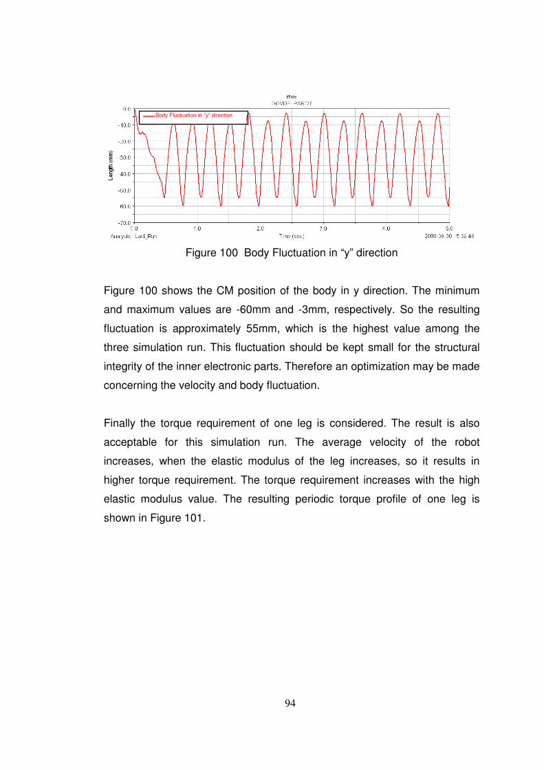
94
Figure 100 Body Fluctuation in “y” direction
Figure 100 shows the CM position of the body in y direction. The minimum
and maximum values are -60mm and -3mm, respectively. So the resulting
fluctuation is approximately 55mm, which is the highest value among the
three simulation run. This fluctuation should be kept small for the structural
integrity of the inner electronic parts. Therefore an optimization may be made
concerning the velocity and body fluctuation.
Finally the torque requirement of one leg is considered. The result is also
acceptable for this simulation run. The average velocity of the robot
increases, when the elastic modulus of the leg increases, so it results in
higher torque requirement. The torque requirement increases with the high
elastic modulus value. The resulting periodic torque profile of one leg is
shown in Figure 101.
Body Fluctuation in “y” direction
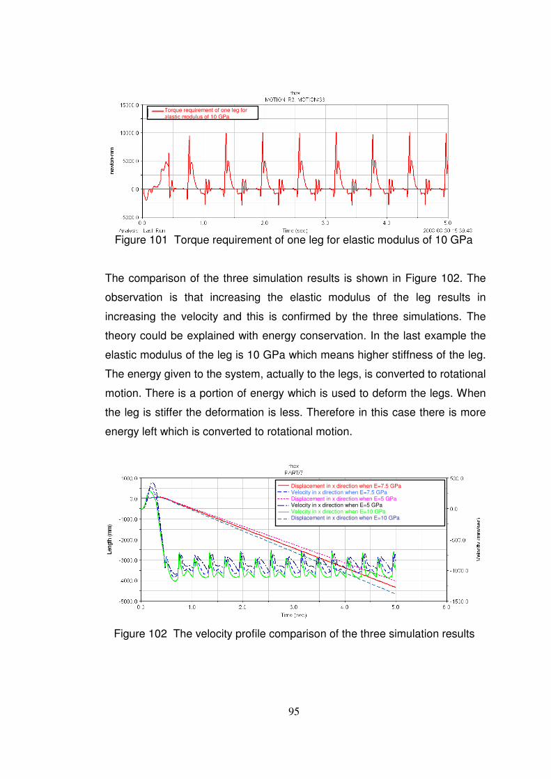
95
Figure 101 Torque requirement of one leg for elastic modulus of 10 GPa
The comparison of the three simulation results is shown in Figure 102. The
observation is that increasing the elastic modulus of the leg results in
increasing the velocity and this is confirmed by the three simulations. The
theory could be explained with energy conservation. In the last example the
elastic modulus of the leg is 10 GPa which means higher stiffness of the leg.
The energy given to the system, actually to the legs, is converted to rotational
motion. There is a portion of energy which is used to deform the legs. When
the leg is stiffer the deformation is less. Therefore in this case there is more
energy left which is converted to rotational motion.
Figure 102 The velocity profile comparison of the three simulation results
Torque requirement of one leg for elastic modulus of 10 GPa
Displacement in x direction when E=7.5 GPa Velocity in x direction when E=7.5 GPa Displacement in x direction when E=5 GPa Velocity in x direction when E=5 GPa Velocity in x direction when E=10 GPa Displacement in x direction when E=10 GPa
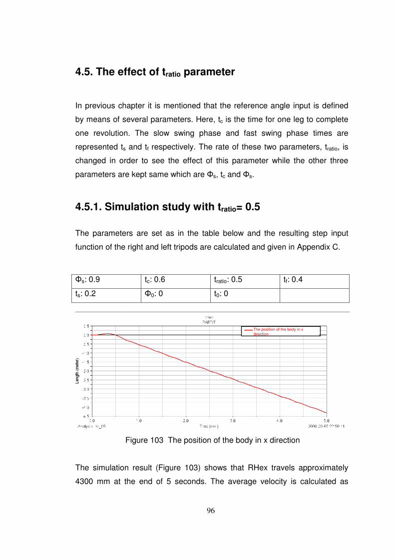
96
4.5. The effect of tratio parameter
In previous chapter it is mentioned that the reference angle input is defined
by means of several parameters. Here, tc is the time for one leg to complete
one revolution. The slow swing phase and fast swing phase times are
represented ts and tf respectively. The rate of these two parameters, tratio, is
changed in order to see the effect of this parameter while the other three
parameters are kept same which are Φs, tc and Φs.
4.5.1. Simulation study with tratio= 0.5
The parameters are set as in the table below and the resulting step input
function of the right and left tripods are calculated and given in Appendix C.
Φs: 0.9 tc: 0.6 tratio: 0.5 tf: 0.4
ts: 0.2 Φ0: 0 t0: 0
Figure 103 The position of the body in x direction
The simulation result (Figure 103) shows that RHex travels approximately
4300 mm at the end of 5 seconds. The average velocity is calculated as
The position of the body in x direction
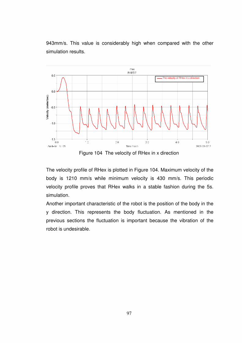
97
943mm/s. This value is considerably high when compared with the other
simulation results.
Figure 104 The velocity of RHex in x direction
The velocity profile of RHex is plotted in Figure 104. Maximum velocity of the
body is 1210 mm/s while minimum velocity is 430 mm/s. This periodic
velocity profile proves that RHex walks in a stable fashion during the 5s.
simulation.
Another important characteristic of the robot is the position of the body in the
y direction. This represents the body fluctuation. As mentioned in the
previous sections the fluctuation is important because the vibration of the
robot is undesirable.
The velocity of RHex in x direction
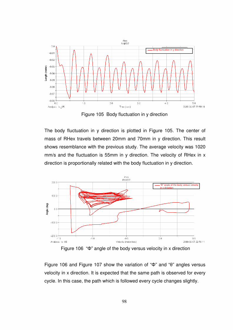
98
Figure 105 Body fluctuation in y direction
The body fluctuation in y direction is plotted in Figure 105. The center of
mass of RHex travels between 20mm and 70mm in y direction. This result
shows resemblance with the previous study. The average velocity was 1020
mm/s and the fluctuation is 55mm in y direction. The velocity of RHex in x
direction is proportionally related with the body fluctuation in y direction.
Figure 106 “Φ” angle of the body versus velocity in x direction
Figure 106 and Figure 107 show the variation of “Φ” and “θ” angles versus
velocity in x direction. It is expected that the same path is observed for every
cycle. In this case, the path which is followed every cycle changes slightly.
Body fluctuation in y direction
“Φ” angle of the body versus velocity in x direction
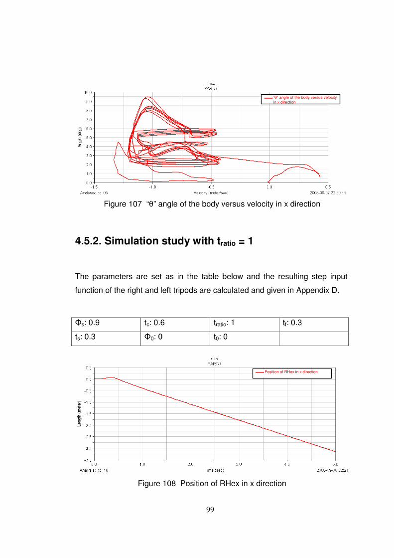
99
Figure 107 “θ” angle of the body versus velocity in x direction
4.5.2. Simulation study with tratio = 1
The parameters are set as in the table below and the resulting step input
function of the right and left tripods are calculated and given in Appendix D.
Φs: 0.9 tc: 0.6 tratio: 1 tf: 0.3
ts: 0.3 Φ0: 0 t0: 0
Figure 108 Position of RHex in x direction
Position of RHex in x direction
“θ” angle of the body versus velocity in x direction
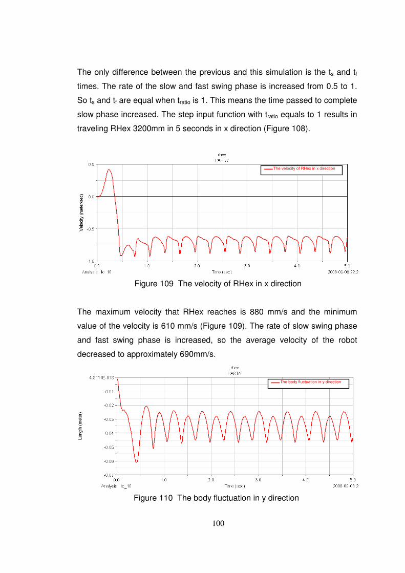
100
The only difference between the previous and this simulation is the ts and tf
times. The rate of the slow and fast swing phase is increased from 0.5 to 1.
So ts and tf are equal when tratio is 1. This means the time passed to complete
slow phase increased. The step input function with tratio equals to 1 results in
traveling RHex 3200mm in 5 seconds in x direction (Figure 108).
Figure 109 The velocity of RHex in x direction
The maximum velocity that RHex reaches is 880 mm/s and the minimum
value of the velocity is 610 mm/s (Figure 109). The rate of slow swing phase
and fast swing phase is increased, so the average velocity of the robot
decreased to approximately 690mm/s.
Figure 110 The body fluctuation in y direction
The velocity of RHex in x direction
The body fluctuation in y direction
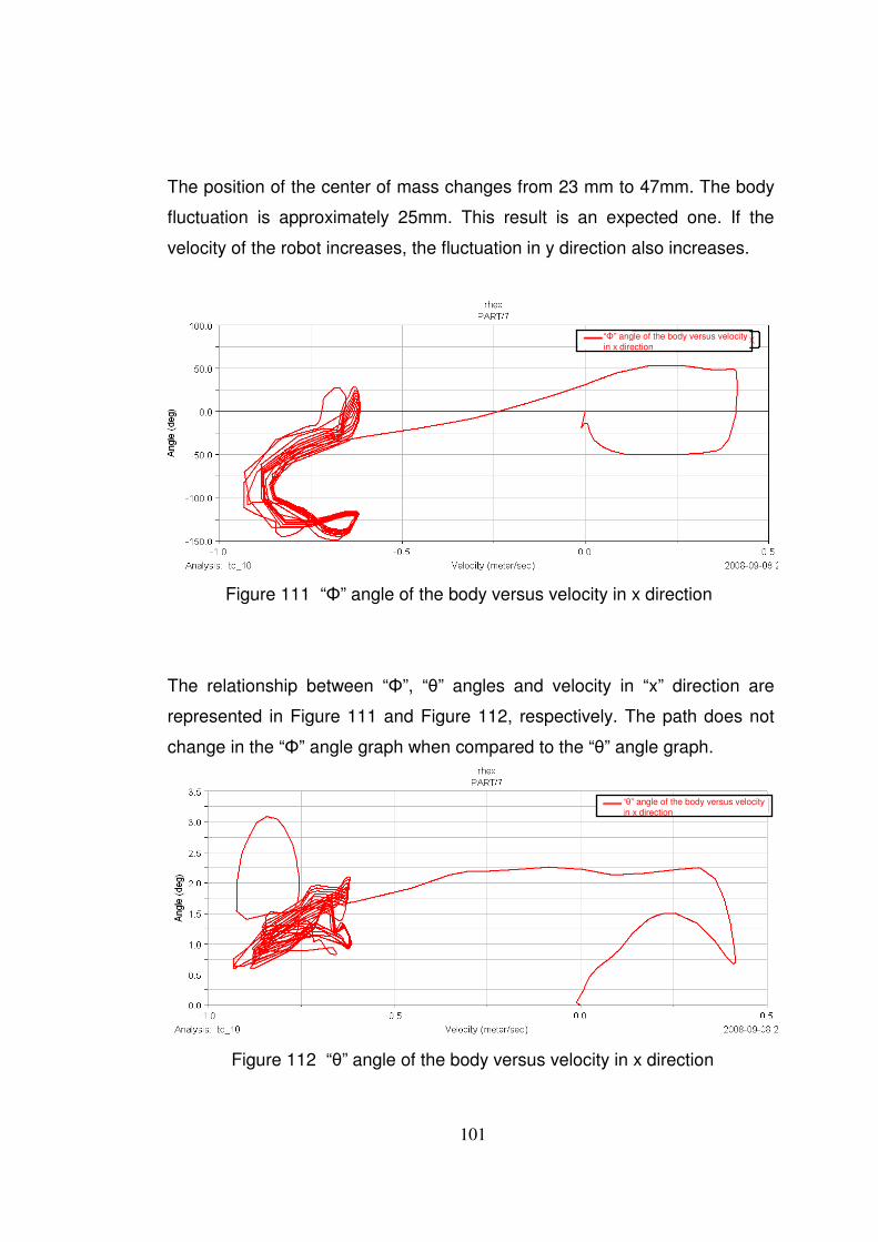
101
The position of the center of mass changes from 23 mm to 47mm. The body
fluctuation is approximately 25mm. This result is an expected one. If the
velocity of the robot increases, the fluctuation in y direction also increases.
Figure 111 “Φ” angle of the body versus velocity in x direction
The relationship between “Φ”, “θ” angles and velocity in “x” direction are
represented in Figure 111 and Figure 112, respectively. The path does not
change in the “Φ” angle graph when compared to the “θ” angle graph.
Figure 112 “θ” angle of the body versus velocity in x direction
“Φ” angle of the body versus velocity in x direction
“θ” angle of the body versus velocity in x direction
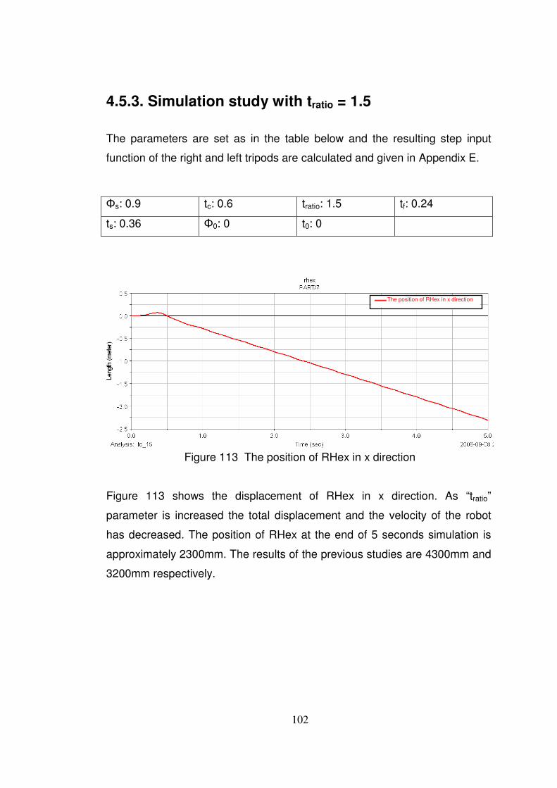
102
4.5.3. Simulation study with tratio = 1.5
The parameters are set as in the table below and the resulting step input
function of the right and left tripods are calculated and given in Appendix E.
Φs: 0.9 tc: 0.6 tratio: 1.5 tf: 0.24
ts: 0.36 Φ0: 0 t0: 0
Figure 113 The position of RHex in x direction
Figure 113 shows the displacement of RHex in x direction. As “tratio”
parameter is increased the total displacement and the velocity of the robot
has decreased. The position of RHex at the end of 5 seconds simulation is
approximately 2300mm. The results of the previous studies are 4300mm and
3200mm respectively.
The position of RHex in x direction

103
Figure 114 The velocity of RHex in x direction
The lowest velocity has occurred in this simulation. The minimum and
maximum velocities are 410mm/s and 640mm/s respectively. The previous
velocity results are 943 mm/s and 690 mm/s while the last study result is 508
mm/s.
Figure 115 The body fluctuation in y direction
The displacement of the center of mass is shown in Figure 115. In this case
the total displacement is approximately 15mm which is the lowest result
among the last three simulations. The relationship between velocity and body
fluctuation is shown one more time, decreasing the velocity results in
decrease of the body fluctuation.
The velocity of RHex in x direction
The body fluctuation in y direction
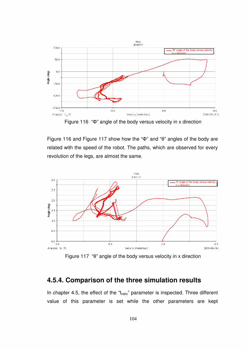
104
Figure 116 “Φ” angle of the body versus velocity in x direction
Figure 116 and Figure 117 show how the “Φ” and “θ” angles of the body are
related with the speed of the robot. The paths, which are observed for every
revolution of the legs, are almost the same.
Figure 117 “θ” angle of the body versus velocity in x direction
4.5.4. Comparison of the three simulation results
In chapter 4.5, the effect of the “tratio” parameter is inspected. Three different
value of this parameter is set while the other parameters are kept
“Φ” angle of the body versus velocity in x direction
“θ” angle of the body versus velocity in x direction
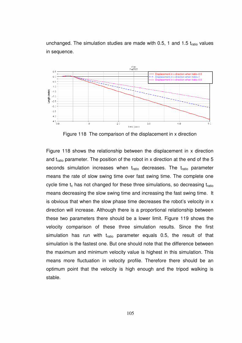
105
unchanged. The simulation studies are made with 0.5, 1 and 1.5 tratio values
in sequence.
Figure 118 The comparison of the displacement in x direction
Figure 118 shows the relationship between the displacement in x direction
and tratio parameter. The position of the robot in x direction at the end of the 5
seconds simulation increases when tratio decreases. The tratio parameter
means the rate of slow swing time over fast swing time. The complete one
cycle time tc has not changed for these three simulations, so decreasing tratio
means decreasing the slow swing time and increasing the fast swing time. It
is obvious that when the slow phase time decreases the robot’s velocity in x
direction will increase. Although there is a proportional relationship between
these two parameters there should be a lower limit. Figure 119 shows the
velocity comparison of these three simulation results. Since the first
simulation has run with tratio parameter equals 0.5, the result of that
simulation is the fastest one. But one should note that the difference between
the maximum and minimum velocity value is highest in this simulation. This
means more fluctuation in velocity profile. Therefore there should be an
optimum point that the velocity is high enough and the tripod walking is
stable.
Displacement in x direction when tratio=0.5 Displacement in x direction when tratio=1 Displacement in x direction when tratio=0.5
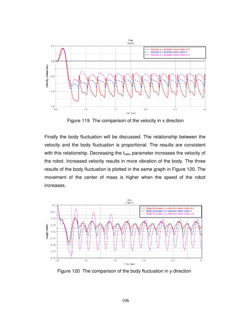
106
Figure 119 The comparison of the velocity in x direction
Finally the body fluctuation will be discussed. The relationship between the
velocity and the body fluctuation is proportional. The results are consistent
with this relationship. Decreasing the tratio parameter increases the velocity of
the robot. Increased velocity results in more vibration of the body. The three
results of the body fluctuation is plotted in the same graph in Figure 120. The
movement of the center of mass is higher when the speed of the robot
increases.
Figure 120 The comparison of the body fluctuation in y direction
Velocity in x direction when tratio=0.5 Velocity in x direction when tratio=1 Velocity in x direction when tratio=1.5
Body fluctuation in y direction when tratio=0.5 Body fluctuation in y direction when tratio=1 Body fluctuation in y direction when tratio=1.5
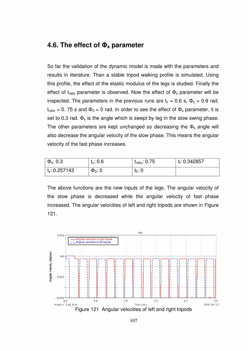
107
4.6. The effect of Φs parameter
So far the validation of the dynamic model is made with the parameters and
results in literature. Than a stable tripod walking profile is simulated. Using
this profile, the effect of the elastic modulus of the legs is studied. Finally the
effect of tratio parameter is observed. Now the effect of Φs parameter will be
inspected. The parameters in the previous runs are tc = 0.6 s, Φs = 0.9 rad,
tratio = 0. 75 s and Φ0 = 0 rad. In order to see the effect of Φs parameter, it is
set to 0.3 rad. Φs is the angle which is swept by leg in the slow swing phase.
The other parameters are kept unchanged so decreasing the Φs angle will
also decrease the angular velocity of the slow phase. This means the angular
velocity of the fast phase increases.
Φs: 0.3 tc: 0.6 tratio: 0.75 tf: 0.342857
ts: 0.257143 Φ0: 0 t0: 0
The above functions are the new inputs of the legs. The angular velocity of
the slow phase is decreased while the angular velocity of fast phase
increased. The angular velocities of left and right tripods are shown in Figure
121.
Figure 121 Angular velocities of left and right tripods
Angular velocities of right tripods Angular velocities of left tripods
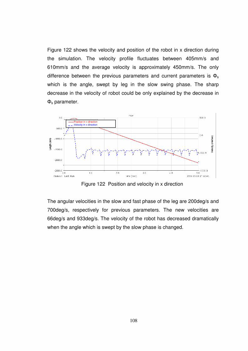
108
Figure 122 shows the velocity and position of the robot in x direction during
the simulation. The velocity profile fluctuates between 405mm/s and
610mm/s and the average velocity is approximately 450mm/s. The only
difference between the previous parameters and current parameters is Φs
which is the angle, swept by leg in the slow swing phase. The sharp
decrease in the velocity of robot could be only explained by the decrease in
Φs parameter.
Figure 122 Position and velocity in x direction
The angular velocities in the slow and fast phase of the leg are 200deg/s and
700deg/s, respectively for previous parameters. The new velocities are
66deg/s and 933deg/s. The velocity of the robot has decreased dramatically
when the angle which is swept by the slow phase is changed.
Position in x direction Velocity in x direction
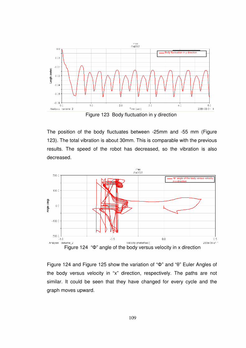
109
Figure 123 Body fluctuation in y direction
The position of the body fluctuates between -25mm and -55 mm (Figure
123). The total vibration is about 30mm. This is comparable with the previous
results. The speed of the robot has decreased, so the vibration is also
decreased.
Figure 124 “Φ” angle of the body versus velocity in x direction
Figure 124 and Figure 125 show the variation of “Φ” and “θ” Euler Angles of
the body versus velocity in “x” direction, respectively. The paths are not
similar. It could be seen that they have changed for every cycle and the
graph moves upward.
Body fluctuation in y direction
“Φ” angle of the body versus velocity in x direction
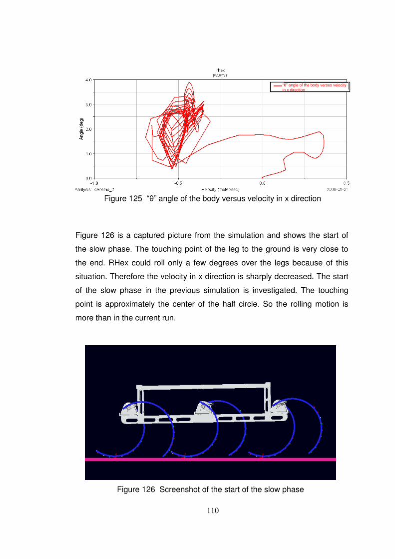
110
Figure 125 “θ” angle of the body versus velocity in x direction
Figure 126 is a captured picture from the simulation and shows the start of
the slow phase. The touching point of the leg to the ground is very close to
the end. RHex could roll only a few degrees over the legs because of this
situation. Therefore the velocity in x direction is sharply decreased. The start
of the slow phase in the previous simulation is investigated. The touching
point is approximately the center of the half circle. So the rolling motion is
more than in the current run.
Figure 126 Screenshot of the start of the slow phase
“θ” angle of the body versus velocity in x direction
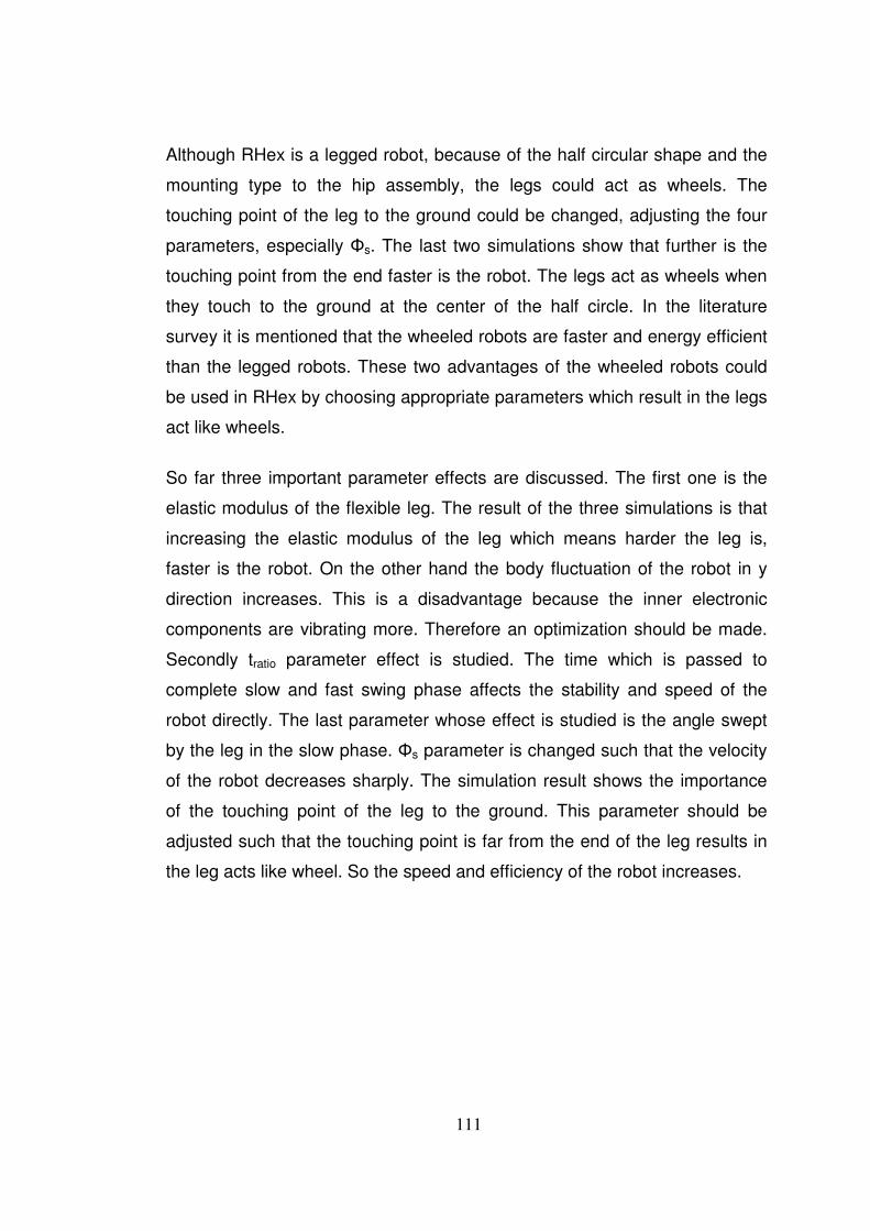
111
Although RHex is a legged robot, because of the half circular shape and the
mounting type to the hip assembly, the legs could act as wheels. The
touching point of the leg to the ground could be changed, adjusting the four
parameters, especially Φs. The last two simulations show that further is the
touching point from the end faster is the robot. The legs act as wheels when
they touch to the ground at the center of the half circle. In the literature
survey it is mentioned that the wheeled robots are faster and energy efficient
than the legged robots. These two advantages of the wheeled robots could
be used in RHex by choosing appropriate parameters which result in the legs
act like wheels.
So far three important parameter effects are discussed. The first one is the
elastic modulus of the flexible leg. The result of the three simulations is that
increasing the elastic modulus of the leg which means harder the leg is,
faster is the robot. On the other hand the body fluctuation of the robot in y
direction increases. This is a disadvantage because the inner electronic
components are vibrating more. Therefore an optimization should be made.
Secondly tratio parameter effect is studied. The time which is passed to
complete slow and fast swing phase affects the stability and speed of the
robot directly. The last parameter whose effect is studied is the angle swept
by the leg in the slow phase. Φs parameter is changed such that the velocity
of the robot decreases sharply. The simulation result shows the importance
of the touching point of the leg to the ground. This parameter should be
adjusted such that the touching point is far from the end of the leg results in
the leg acts like wheel. So the speed and efficiency of the robot increases.
112
CHAPTER 5
CONCLUSION
The aim of this study is to build a virtual prototype of RHex robot. As is
known, RHex is a hexapod robot with flexible legs, which are manufactured
from composite material with a special process. Therefore the dynamic
model of RHex should include compliant parts. This means a dynamic
simulation program should interact with a finite element software. MSC
ADAMS is used in order to build the dynamic model. The flexible members
are added with the use of MSC PATRAN and MSC NASTRAN programs. At
this stage the flexible multi body dynamic model is ready to simulate RHex.
Finally it is needed to control the robot with a control structure. The real case
could be fully simulated after completing the ADAMS – MATLAB interaction.
A closed loop control structure is built in MATLAB, which also includes the
motor model.
First, the model is tested with the results in literature. In this case MATLAB
interaction is not included, because the validation of the model should be
made. The parameters in literature are set and a simulation run has been
performed. The results in literature are for the previous version of RHex. The
differences are that the body dimensions, motors, weight and flexible leg
dimensions and properties have been changed. The simulation results are
comparable with results in literature considering the version difference of the
robot.
Second, MATLAB program is included as a closed loop controller. In that
case the solver types and step times are very important. The synchronization
of the two programs should be adjusted very carefully. Otherwise the
113
controller could not be able to follow the reference angular velocity. ADAMS
software has only one solver type, fixed step. There are two choices. One is
that MATLAB solves the dynamic model and the controller equations. The
second choice is that ADAMS solves the dynamic model and MATLAB deals
with the controller part. The two choices are tried to simulate the dynamic
model. In both cases step time should be less than 0.00005s. This results in
enormous number of equations and huge simulation time. A “3s. simulation”
is performed in order to see that the controller could follow the reference
angular position input accurately. Although the result is satisfactory, the error
between the real and reference angular position is less than 0.01 rad., the
total simulation has taken place in approximately 3 days. Therefore the other
simulation trials do not include MATLAB, closed loop controller.
A stable tripod walking parameter set is found and used for inspecting the
effect of the elastic modulus of the flexible legs. The elastic modulus of the
flexible legs is calculated as 10 GPa. Three simulations are performed with
three different elastic modulus values, 5 GPa, 7.5 GPa, 10 GPa. The results
show that if the elastic modulus is higher, the velocity of the robot would
increase. Another observation is about the body fluctuation. The position of
the center of mass is plotted. This parameter is important because vibration
of the electronic components is not wanted. The plotted graphs show the
speed of the robot is directly related with the body fluctuation. When the
speed of the robot increases, so does the fluctuation. Therefore an
optimization can be made here. In these three case studies, the torque
requirements are observed. MATLAB is not included for these simulations; so
it is assumed that the reference angular position is exactly followed and
motor torque is unlimited. Therefore torque graphs are very important. The
torque speed curve of the motor is used as a reference in order to see that
the torque requirement could be afforded by the motors. It is seen that the
peaks of the torque graphs is less than the motor maximum torque. So, as a
result, if MATLAB was included in this simulation there should be minimal
differences in the behavior of the robot.
114
Another parameter, traito, is inspected in order to see its effect. Actually the
four parameters which are used to define the reference angular position are
tc, ts, Φs, Φ0. “traito” is not one of them. It is the ratio of the slow swing time, ts,
over fast swing time, tf. A meaningful parameter is tried to derive. This ratio is
set 0.5, 1 and 1,5 respectively and three simulations are performed. The
results are inspected to comment on the effect of this parameter. The
increase of traito parameter means decreasing the fast swing time. Although
the time which is passed to complete one revolution of the leg, tc, is kept
unchanged, decreasing tratio parameter results in increase of the speed of the
robot. It is related with the difference between slow and fast swing angular
velocities. If this difference increases, the speed of the robot decreases
dramatically.
Finally the effect of Φs parameter is inspected. This parameter defines the
angle which is swept by the slow swing phase. It is more related with the
touching point of the leg to the ground. So far Φs parameter is used as 0.9
rad. and in this trial the parameter is set to 0.3 rad. In this case the touching
point of the leg to the ground is very close to the end of the leg. This results
in decreasing of the speed of the robot. Farther the touching point from the
end of the leg, higher is the velocity in “x” direction. At this stage, the rolling
motion increases the speed of the robot.
So far a virtual prototype of RHex robot is built and the validation of this
model is done. Then a stable tripod walking parameter set is found. The
effects of leg stiffness, tratio and Φs parameters are inspected using the stable
parameter set, while the other parameters are kept unchanged. The behavior
of the RHex robot is observed under different circumstances.
For future work the refinement of this model could be made in order to
decrease the simulation time. In that case a mathematical approach could be
used in order to find the most efficient stable tripod walking parameters with
running multiple simulations.
115
REFERENCES
[1] Manuel F. Silva and J.A. Tenreiro Machado. A Historical Perspective of
Legged Robots. Journal of Vibration and Control 2007; 13; 1447
[2] Rosheim M. E., 1994, Robot Evolution: The Development of Anthrobotics,
1st edition, Wiley, New York
[3] K. J. Waldron and V. J. Vohnout. Configuration design of the Adaptive
Suspension Vehicle. International Journal of Robotics Research, 3(2):37{48,
1984
[4] Saranli, U., Dynamic locomotion with a Hexapod Robot, A dissertation
submitted in partial fulfillment of the requirements for the degree of Doctor of
Philosophy, Computer Science and Engineering in The University of
Michigan, 2002
[5] Bekker, M. G., 1960, Off-The-Road Locomotion, University of Michigan
Press, Ann Arbor, MI.
[6] Kaneko, M., Mizuno, A. and Harada, K., 2002, “Torque distribution for
achieving a hugging walk,” in Proceedings of the 2002 IEEE/RSJ
International Conference on Intelligent Robots and Systems, Lausanne,
Switzerland, September 30–October 4, pp. 2613–2618
[7] Yang, J.-M. and Kim, J.-H., 1998, “A strategy of optimal fault tolerant gait
for the hexapod robot in crab walking,” in Proceedings of the 1998 IEEE
International Conference on Robotics and Automation, Leuven, Belgium, May
16–20, pp. 1695–1700
116
[8] Hirose, S. and Kato, K., 1998, “Development of quadruped walking robot
with the mission of mine detection and removal – proposal of shape-feedback
master-slave arm,” in Proceedings of the 1998 IEEE International
Conference on Robotics and Automation, Leuven, Belgium, May 16–20, pp.
1713–1718
[9] Lee, Y.-J. and Hirose, S., 2000, “Three-legged walking for fault tolerant
locomotion of a quadruped robot with demining mission,” in Proceedings of
the 2000 IEEE/RSJ International Conference on Intelligent Robots and
Systems, Takamatsu, Japan, October 30–November 5, pp. 973–978
[10] Yang, J.-M., 2003, “Fault-tolerant gait generation for locked joint
failures,” in Proceedings of the 2003 IEEE International Conference on
Systems, Man and Cybernetics, Washington, DC, USA, October 5–8, pp.
2237–2242.
[11] Spenneberg, D., McCullough, K., and Kirchner, F., 2004, “Stability of
walking in a multilegged robot suffering leg loss,” in Proceedings of the 2004
IEEE International Conference on Robotics and Automation, NewOrleans,
LA, April 26–May 1, pp. 2159–2164
[12] Nonami, K. and Huang, Q.-J., 2001, “Humanitarian mine detection six-
legged walking robot COMET-II with two manipulators,” in Proceedings
CLAWAR’2001 – 4th International Conference on Climbing and Walking
Robots, Karlsruhe, Germany, September 24–26, pp. 989–996.
[13] Ihme, T., 2003, “Posture control and distributed force sensing for
technical applications of walking robots,” in Proceedings of the ICAR 2003 –
11th International Conference on Advanced Robotics, Coimbra, Portugal,
June 30–July 3, pp. 1032–1037.
117
[14] Takita, K., Katayama, T., and Hirose, S., 2003, “Development of
dinosaur-like robot TITRUS–the efficacy of the neck and tail of miniature
dinosaur-like robot TITRUS-III,” in Proceedings of the 2003 IEEE
International Conference on Robotics and Automation, Taipei, Taiwan,
September 14–19, pp. 2466–2471.
[15] Hirose, S. and Kato, K., 1998, “Development of quadruped walking robot
with the mission of mine detection and removal – proposal of shape-feedback
master-slave arm,” in Proceedings of the 1998 IEEE International
Conference on Robotics and Automation, Leuven, Belgium, May 16–20, pp.
1713–1718.
[16] Omata, T., Tsukagoshi, K., and Mori, O., 2002, “Whole quadruped
manipulation,” in Proceedings of the 2002 IEEE International Conference on
Robotics and Automation, Washington, DC, May 11–15, pp. 2028–2033.
[17] Takahashi, Y., Arai, T., Mae, Y., Inoue, K., and Koyachi, N., 2000,
“Development of multi-limb robot with omnidirectional manipulability and
mobility,” in Proceedings of the 2000 IEEE/RSJ International Conference on
Intelligent Robots and Systems, Takamatsu, Japan, October 30–November
5, pp. 2012–2017.
[18] Koyachi, N., Adachi, H., Senjo, N., Murata, R., Izumi, M., Hirose, T., and
Arai, T., 2002, “Control of walk and manipulation by a hexapod with
integrated limb mechanism: MELMANTIS-1,” in Proceedings of the 2002
IEEE International Conference on Robotics and Automation, Washington,
DC, May 11–15, pp. 3553–3558.
[19] Janrathitikarn,O., The Use of a Cognitive Architecture To Control A Six-
legged Robot, A dissertation submitted in Partial Fulfillment of the
Requirements for the Degree of Master of Science, Aerospace Engineering
in The Pennsylvania State University,2007.
118
[20] Matsuoka, K., 1979, “A model of repetitive hopping movements in man,”
in Fifth World Congress on Theory of Machines and Mechanisms,
International Federation for Information Processing
[21] Raibert, M. H., 1986, Legged Robots that Balance, The MIT Press,
Cambridge, MA.
[22] Ahmadi, M. and Buehler, M., 2006, “Controlled passive dynamic running
experiments with ARL Monopod II,” IEEE Transactions on Robotics 22(5),
974–986
[23] Iida, F., Dravid, R., and Paul, C., 2002, “Design and control of a
pendulum driven hopping robot,” in Proceedings of the 2002 IEEE/RSJ
International Conference on Intelligent Robots and Systems, Lausanne,
Switzerland, September 30–October 4, pp. 2141–2146
[24] Hirai, K., Hirose, M., Haikawa, Y. and Takenaka, T., 1998, “The
development of Honda humanoid robot,” in Proceedings of the 1998 IEEE
International Conference on Robotics and Automation, Leuven, Belgium, May
16–20, pp. 1321–1326.
[25] Sakagami, Y., Watanabe, R., Aoyama, C., Matsunaga, S., Higaki, N.,
and Fujimura, K., 2002, “The intelligent ASIMO: system overview and
integration,” in Proceedings of the 2002 IEEE/RSJ International Conference
on Intelligent Robots and Systems, Lausanne, Switzerland, September 30–
October 4, pp. 2478–2483.
[26] P. G. d. Santos, E. Garcia, and J. Estremera, "Quadrupedal locomotion:
An introduction to the control four-legged robots," Germany: Springer, 2006,
pp. 3, 29-31.
119
[27] D. J. Todd, Walking Machines: An Introduction to Legged Robots. New
York: Chapman and Hall,1985.
[28] Raibert, M. H., 1986, Legged Robots that Balance, The MIT Press,
Cambridge, MA.
[29] Liston, R. A. and Mosher, R. S., 1968, “A Versatile Walking Truck,” in
Proceedings of the Transportation Engineering Conference, Institute of Civil
Engineers, London.
[30] Mosher, R. S., 1968, “Test and evaluation of a versatile walking truck,” in
Proceedings of the Off-Road Mobility Research Symposium, International
Society for Terrain Vehicle Systems, Washington, DC, May, pp. 359–379.
[31] McGhee, R. B., 1966, “Finite state control of quadruped locomotion,” in
Second International Symposium on External Control of Extremities.
[32] Frank, A. A., 1968, Automatic Control Systems for Legged Locomotion.
USCEE Report No. 273, University of Southern California, Los Angeles, CA.
[33] Buehler, M., Cocosco, A., Yamazaki, K., and Battaglia, R., 1999, “Stable
open loop walking in quadruped robots with stick legs,” in Proceedings of the
1999 IEEE International Conference on Robotics and Automation, Detroit,
MI, May 10–15, pp. 2348–2353.
[34] Poulakakis, I., Smith, J. A., and Buehler, M., 2005, “Modeling and
experiments of untethered quadrupedal running with a bounding gait: The
Scout II robot,” International Journal of Robotics Research 24(4), 239–256.
[35] Papadopoulos, D. and Buehler,M., 2000, “Stable running in a quadruped
robot with compliant legs,” in Proceedings of the 2000 IEEE International
120
Conference on Robotics and Automation, San Francisco, CA, April 24–28,
pp. 444–449.
[36] Hawker, G. and Buehler, M., 2000, “Quadruped trotting with passive
knees–design, control, and experiments,” in Proceedings of the 2000 IEEE
International Conference on Robotics and Automation, San Francisco, CA,
April 24–28, pp. 3046–3051.
[37] A. A. Yumaryanto, J. An, and L. Sangyoon, "A cockroach-inspired
hexapod robot actuated by LIPCA," in IEEE Conference on Robotics,
Automation and Mechatronics, 2006, pp. 1-6.
[38] P. G. d. Santos, E. Garcia, and J. Estremera, "Quadrupedal locomotion:
An introduction to the control four-legged robots," Germany: Springer, 2006,
pp. 3, 29-31.
[39] D. J. Todd, Walking Machines: An Introduction to Legged Robots. New
York: Chapman and Hall, 1985.
[40] F. Ozguner and S.-J, 1985. Tsai, "Design and implementation of a
binocular-vision system for locating footholds of a multi-legged walking
robot," IEEE Transactions on Industrial Electronics, vol. IE- 32, pp. 26-31,
[41] Binnard,M. B., 1995, Design of a Small PneumaticWalking Robot.MSc
thesis,Massachusetts Institute of Technology – Department of Mechanical
Engineering, Cambridge, MA.
[42] Pfeiffer, F., Eltze, J., and Weidemann, H.-J., 1995, “The TUM-walking
machine,” Intelligent Automation and Soft Computing 1(3), 307–323.
[43] Quinn, R. D., Offi, J. T., Kingsley, D. A., and Ritzmann, R. E., 2002,
“Improved mobility through abstracted biological principles,” in Proceedings
121
of the 2002 IEEE/RSJ International Conference on Intelligent Robots and
Systems, Lausanne, Switzerland, September 30–October 4, pp. 2652–2657.
[44] Saranli, U., Buehler, M., and Koditschek, D. E., 2001, “RHex–a simple
and highly mobile hexapod robot,” The International Journal of Robotics
Research 20(7), 616–631.
[45] Potesil, A., Hanzlik, V. Application of Expert Systems ANSYS and
ADAMS in Optimization of Mechanisms With Elastic Member
[46] Albers, A., Emmrich, D. and Häußler, P. Automated Structural
Optimization of Flexible Components using MSC.Adams/Flex and
MSC.Nastran Sol200
[47] Joldes, G. R., Improved Linear Tetrahedral Element for Surgical
Simulation, Intelligent Systems for Medicine Lab., The University of Western
Australia
[48] R.J. Pulles Controller Design for ADAMS models using
MATLAB/SIMULINK interaction DCT-2003-29
[49] Maxon motor, RE 30 _30 mm, Graphite Brushes, 60 Watt catalog.
www.maxonmotor.com
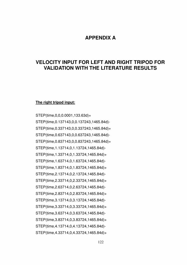
122
APPENDIX A
VELOCITY INPUT FOR LEFT AND RIGHT TRIPOD FOR VALIDATION WITH THE LITERATURE RESULTS
The right tripod input:
STEP(time,0,0,0.0001,133.63d)+
STEP(time,0.137143,0,0.137243,1465.84d)-
STEP(time,0.337143,0,0.337243,1465.84d)+
STEP(time,0.637143,0,0.637243,1465.84d)-
STEP(time,0.837143,0,0.837243,1465.84d)+
STEP(time,1.13714,0,1.13724,1465.84d)-
STEP(time,1.33714,0,1.33724,1465.84d)+
STEP(time,1.63714,0,1.63724,1465.84d)-
STEP(time,1.83714,0,1.83724,1465.84d)+
STEP(time,2.13714,0,2.13724,1465.84d)-
STEP(time,2.33714,0,2.33724,1465.84d)+
STEP(time,2.63714,0,2.63724,1465.84d)-
STEP(time,2.83714,0,2.83724,1465.84d)+
STEP(time,3.13714,0,3.13724,1465.84d)-
STEP(time,3.33714,0,3.33724,1465.84d)+
STEP(time,3.63714,0,3.63724,1465.84d)-
STEP(time,3.83714,0,3.83724,1465.84d)+
STEP(time,4.13714,0,4.13724,1465.84d)-
STEP(time,4.33714,0,4.33724,1465.84d)+
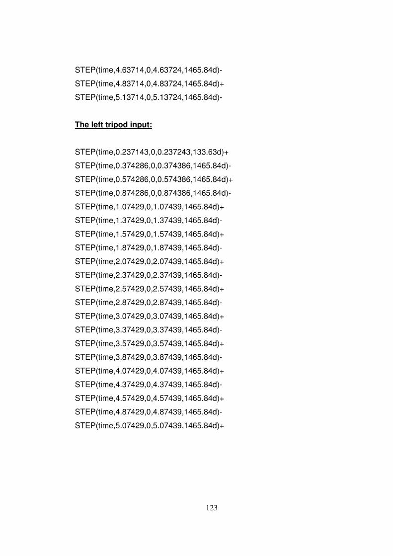
123
STEP(time,4.63714,0,4.63724,1465.84d)-
STEP(time,4.83714,0,4.83724,1465.84d)+
STEP(time,5.13714,0,5.13724,1465.84d)-
The left tripod input:
STEP(time,0.237143,0,0.237243,133.63d)+
STEP(time,0.374286,0,0.374386,1465.84d)-
STEP(time,0.574286,0,0.574386,1465.84d)+
STEP(time,0.874286,0,0.874386,1465.84d)-
STEP(time,1.07429,0,1.07439,1465.84d)+
STEP(time,1.37429,0,1.37439,1465.84d)-
STEP(time,1.57429,0,1.57439,1465.84d)+
STEP(time,1.87429,0,1.87439,1465.84d)-
STEP(time,2.07429,0,2.07439,1465.84d)+
STEP(time,2.37429,0,2.37439,1465.84d)-
STEP(time,2.57429,0,2.57439,1465.84d)+
STEP(time,2.87429,0,2.87439,1465.84d)-
STEP(time,3.07429,0,3.07439,1465.84d)+
STEP(time,3.37429,0,3.37439,1465.84d)-
STEP(time,3.57429,0,3.57439,1465.84d)+
STEP(time,3.87429,0,3.87439,1465.84d)-
STEP(time,4.07429,0,4.07439,1465.84d)+
STEP(time,4.37429,0,4.37439,1465.84d)-
STEP(time,4.57429,0,4.57439,1465.84d)+
STEP(time,4.87429,0,4.87439,1465.84d)-
STEP(time,5.07429,0,5.07439,1465.84d)+
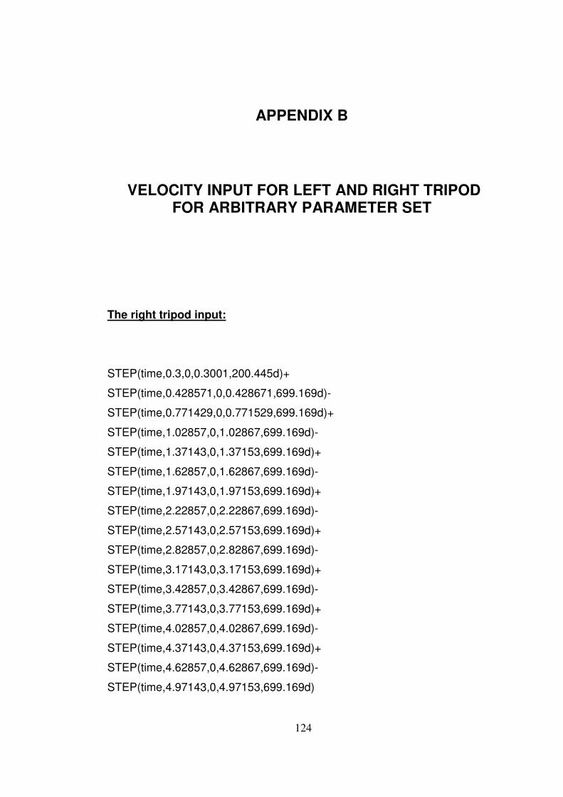
124
APPENDIX B
VELOCITY INPUT FOR LEFT AND RIGHT TRIPOD FOR ARBITRARY PARAMETER SET
The right tripod input:
STEP(time,0.3,0,0.3001,200.445d)+
STEP(time,0.428571,0,0.428671,699.169d)-
STEP(time,0.771429,0,0.771529,699.169d)+
STEP(time,1.02857,0,1.02867,699.169d)-
STEP(time,1.37143,0,1.37153,699.169d)+
STEP(time,1.62857,0,1.62867,699.169d)-
STEP(time,1.97143,0,1.97153,699.169d)+
STEP(time,2.22857,0,2.22867,699.169d)-
STEP(time,2.57143,0,2.57153,699.169d)+
STEP(time,2.82857,0,2.82867,699.169d)-
STEP(time,3.17143,0,3.17153,699.169d)+
STEP(time,3.42857,0,3.42867,699.169d)-
STEP(time,3.77143,0,3.77153,699.169d)+
STEP(time,4.02857,0,4.02867,699.169d)-
STEP(time,4.37143,0,4.37153,699.169d)+
STEP(time,4.62857,0,4.62867,699.169d)-
STEP(time,4.97143,0,4.97153,699.169d)
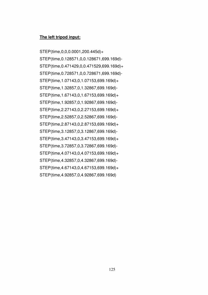
125
The left tripod input:
STEP(time,0,0,0.0001,200.445d)+
STEP(time,0.128571,0,0.128671,699.169d)-
STEP(time,0.471429,0,0.471529,699.169d)+
STEP(time,0.728571,0,0.728671,699.169d)-
STEP(time,1.07143,0,1.07153,699.169d)+
STEP(time,1.32857,0,1.32867,699.169d)-
STEP(time,1.67143,0,1.67153,699.169d)+
STEP(time,1.92857,0,1.92867,699.169d)-
STEP(time,2.27143,0,2.27153,699.169d)+
STEP(time,2.52857,0,2.52867,699.169d)-
STEP(time,2.87143,0,2.87153,699.169d)+
STEP(time,3.12857,0,3.12867,699.169d)-
STEP(time,3.47143,0,3.47153,699.169d)+
STEP(time,3.72857,0,3.72867,699.169d)-
STEP(time,4.07143,0,4.07153,699.169d)+
STEP(time,4.32857,0,4.32867,699.169d)-
STEP(time,4.67143,0,4.67153,699.169d)+
STEP(time,4.92857,0,4.92867,699.169d)
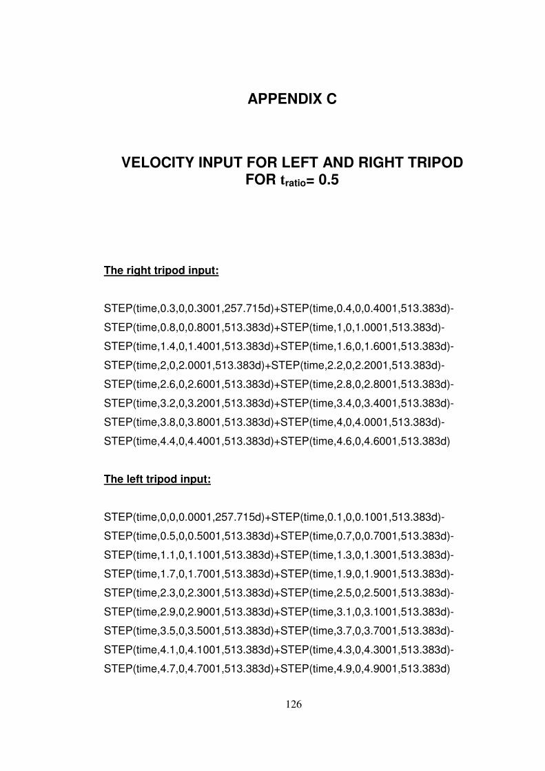
126
APPENDIX C
VELOCITY INPUT FOR LEFT AND RIGHT TRIPOD FOR tratio= 0.5
The right tripod input:
STEP(time,0.3,0,0.3001,257.715d)+STEP(time,0.4,0,0.4001,513.383d)-
STEP(time,0.8,0,0.8001,513.383d)+STEP(time,1,0,1.0001,513.383d)-
STEP(time,1.4,0,1.4001,513.383d)+STEP(time,1.6,0,1.6001,513.383d)-
STEP(time,2,0,2.0001,513.383d)+STEP(time,2.2,0,2.2001,513.383d)-
STEP(time,2.6,0,2.6001,513.383d)+STEP(time,2.8,0,2.8001,513.383d)-
STEP(time,3.2,0,3.2001,513.383d)+STEP(time,3.4,0,3.4001,513.383d)-
STEP(time,3.8,0,3.8001,513.383d)+STEP(time,4,0,4.0001,513.383d)-
STEP(time,4.4,0,4.4001,513.383d)+STEP(time,4.6,0,4.6001,513.383d)
The left tripod input:
STEP(time,0,0,0.0001,257.715d)+STEP(time,0.1,0,0.1001,513.383d)-
STEP(time,0.5,0,0.5001,513.383d)+STEP(time,0.7,0,0.7001,513.383d)-
STEP(time,1.1,0,1.1001,513.383d)+STEP(time,1.3,0,1.3001,513.383d)-
STEP(time,1.7,0,1.7001,513.383d)+STEP(time,1.9,0,1.9001,513.383d)-
STEP(time,2.3,0,2.3001,513.383d)+STEP(time,2.5,0,2.5001,513.383d)-
STEP(time,2.9,0,2.9001,513.383d)+STEP(time,3.1,0,3.1001,513.383d)-
STEP(time,3.5,0,3.5001,513.383d)+STEP(time,3.7,0,3.7001,513.383d)-
STEP(time,4.1,0,4.1001,513.383d)+STEP(time,4.3,0,4.3001,513.383d)-
STEP(time,4.7,0,4.7001,513.383d)+STEP(time,4.9,0,4.9001,513.383d)
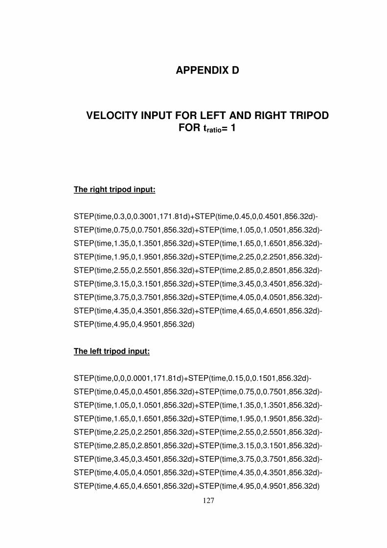
127
APPENDIX D
VELOCITY INPUT FOR LEFT AND RIGHT TRIPOD FOR tratio= 1
The right tripod input:
STEP(time,0.3,0,0.3001,171.81d)+STEP(time,0.45,0,0.4501,856.32d)-
STEP(time,0.75,0,0.7501,856.32d)+STEP(time,1.05,0,1.0501,856.32d)-
STEP(time,1.35,0,1.3501,856.32d)+STEP(time,1.65,0,1.6501,856.32d)-
STEP(time,1.95,0,1.9501,856.32d)+STEP(time,2.25,0,2.2501,856.32d)-
STEP(time,2.55,0,2.5501,856.32d)+STEP(time,2.85,0,2.8501,856.32d)-
STEP(time,3.15,0,3.1501,856.32d)+STEP(time,3.45,0,3.4501,856.32d)-
STEP(time,3.75,0,3.7501,856.32d)+STEP(time,4.05,0,4.0501,856.32d)-
STEP(time,4.35,0,4.3501,856.32d)+STEP(time,4.65,0,4.6501,856.32d)-
STEP(time,4.95,0,4.9501,856.32d)
The left tripod input:
STEP(time,0,0,0.0001,171.81d)+STEP(time,0.15,0,0.1501,856.32d)-
STEP(time,0.45,0,0.4501,856.32d)+STEP(time,0.75,0,0.7501,856.32d)-
STEP(time,1.05,0,1.0501,856.32d)+STEP(time,1.35,0,1.3501,856.32d)-
STEP(time,1.65,0,1.6501,856.32d)+STEP(time,1.95,0,1.9501,856.32d)-
STEP(time,2.25,0,2.2501,856.32d)+STEP(time,2.55,0,2.5501,856.32d)-
STEP(time,2.85,0,2.8501,856.32d)+STEP(time,3.15,0,3.1501,856.32d)-
STEP(time,3.45,0,3.4501,856.32d)+STEP(time,3.75,0,3.7501,856.32d)-
STEP(time,4.05,0,4.0501,856.32d)+STEP(time,4.35,0,4.3501,856.32d)-
STEP(time,4.65,0,4.6501,856.32d)+STEP(time,4.95,0,4.9501,856.32d)
128
APPENDIX E
VELOCITY INPUT FOR LEFT AND RIGHT TRIPOD FOR tratio= 1.5
The right tripod input:
STEP(time,0.3,0,0.3001,143.175d)+STEP(time,0.48,0,0.4801,1141.99d)-
STEP(time,0.72,0,0.7201,1141.99d)+STEP(time,1.08,0,1.0801,1141.99d)-
STEP(time,1.32,0,1.3201,1141.99d)+STEP(time,1.68,0,1.6801,1141.99d)-
STEP(time,1.92,0,1.9201,1141.99d)+STEP(time,2.28,0,2.2801,1141.99d)-
STEP(time,2.52,0,2.5201,1141.99d)+STEP(time,2.88,0,2.8801,1141.99d)-
STEP(time,3.12,0,3.1201,1141.99d)+STEP(time,3.48,0,3.4801,1141.99d)-
STEP(time,3.72,0,3.7201,1141.99d)+STEP(time,4.08,0,4.0801,1141.99d)-
STEP(time,4.32,0,4.3201,1141.99d)+STEP(time,4.68,0,4.6801,1141.99d)-
STEP(time,4.92,0,4.9201,1141.99d)
The left tripod input:
STEP(time,0,0,0.0001,143.175d)+STEP(time,0.18,0,0.1801,1141.99d)-
STEP(time,0.42,0,0.4201,1141.99d)+STEP(time,0.78,0,0.7801,1141.99d)-
STEP(time,1.02,0,1.0201,1141.99d)+STEP(time,1.38,0,1.3801,1141.99d)-
STEP(time,1.62,0,1.6201,1141.99d)+STEP(time,1.98,0,1.9801,1141.99d)-
STEP(time,2.22,0,2.2201,1141.99d)+STEP(time,2.58,0,2.5801,1141.99d)-
STEP(time,2.82,0,2.8201,1141.99d)+STEP(time,3.18,0,3.1801,1141.99d)-
STEP(time,3.42,0,3.4201,1141.99d)+STEP(time,3.78,0,3.7801,1141.99d)-
STEP(time,4.02,0,4.0201,1141.99d)+STEP(time,4.38,0,4.3801,1141.99d)-
STEP(time,4.62,0,4.6201,1141.99d)+STEP(time,4.98,0,4.9801,1141.99d)
129
APPENDIX F
VELOCITY INPUT FOR LEFT AND RIGHT TRIPOD FOR Φs PARAMETER
The right tripod input:
STEP(time,0.3,0,0.3001,66.815d)+
STEP(time,0.428571,0,0.428671,933.021d)-
STEP(time,0.771429,0,0.771529,933.021d)+
STEP(time,1.02857,0,1.02867,933.021d)-
STEP(time,1.37143,0,1.37153,933.021d)+
STEP(time,1.62857,0,1.62867,933.021d)-
STEP(time,1.97143,0,1.97153,933.021d)+
STEP(time,2.22857,0,2.22867,933.021d)-
STEP(time,2.57143,0,2.57153,933.021d)+
STEP(time,2.82857,0,2.82867,933.021d)-
STEP(time,3.17143,0,3.17153,933.021d)+
STEP(time,3.42857,0,3.42867,933.021d)-
STEP(time,3.77143,0,3.77153,933.021d)+
STEP(time,4.02857,0,4.02867,933.021d)-
STEP(time,4.37143,0,4.37153,933.021d)+
STEP(time,4.62857,0,4.62867,933.021d)-
STEP(time,4.97143,0,4.97153,933.021d)

130
The left tripod input:
STEP(time,0,0,0.0001,66.815d)+
STEP(time,0.128571,0,0.128671,933.021d)-
STEP(time,0.471429,0,0.471529,933.021d)+
STEP(time,0.728571,0,0.728671,933.021d)-
STEP(time,1.07143,0,1.07153,933.021d)+
STEP(time,1.32857,0,1.32867,933.021d)-
STEP(time,1.67143,0,1.67153,933.021d)+
STEP(time,1.92857,0,1.92867,933.021d)-
STEP(time,2.27143,0,2.27153,933.021d)+
STEP(time,2.52857,0,2.52867,933.021d)-
STEP(time,2.87143,0,2.87153,933.021d)+
STEP(time,3.12857,0,3.12867,933.021d)-
STEP(time,3.47143,0,3.47153,933.021d)+
STEP(time,3.72857,0,3.72867,933.021d)-
STEP(time,4.07143,0,4.07153,933.021d)+
STEP(time,4.32857,0,4.32867,933.021d)-
STEP(time,4.67143,0,4.67153,933.021d)+
STEP(time,4.92857,0,4.92867,933.021d)