fixed-income portfolio optimization based on dynamic ... · modeling and forecasting the term...

Fixed-income portfolio optimization based on dynamic Nelson-Siegel models with

macroeconomic factors for the Brazilian yield curve

Richard Schnorrenberger∗ Guilherme Valle Moura†

AbstractThe study investigates the statistical and economic value of forecasted yields generated by dynamicyield curve models which incorporate a large macroeconomic dataset. The analysis starts off bymodeling and forecasting the term structure of the Brazilian nominal interest rates using severalspecifications for the dynamic Nelson-Siegel (DNS) framework, suggested by Diebold and Li (2006).The comparison of forecast performance for forecast horizons above three months supports theevidence for the incorporation of one macroeconomic factor that summarizes broad informationregarding mainly inflation expectations. In order to assess the economic value of those forecastedyields, a fixed-income portfolio optimization using the mean-variance approach of Markowitz (1952) isperformed. The analysis indicate that good yield curve predictions are important to achieve economicgains from forecasted yields in terms of portfolio performance. Preferred forecasted yields for shortforecast horizons perform quite well for optimal mean-variance portfolios with one-step-aheadestimates for fixed-income returns, while forecasted yields generated by a macroeconomic DNSspecification outperforms in terms of portfolio performance with six-step-ahead estimates. Therefore,there is an economic and statistical gain from considering a large macroeconomic dataset to forecast theBrazilian yield curve dynamics, specially for longer forecast horizons.

Keywords: Fixed-income portfolio optimization. Brazilian yield curve. Dynamic Nelson-Siegel model.Macroeconomic factors. Yield curve forecasting. Mean-variance approach.

ResumoO estudo investiga o valor estatístico e econômico dos rendimentos previstos por modelos dinâmicos dacurva de juros que incorporam um grande conjunto de dados macroeconômicos. A análise parte damodelagem e previsão da estrutura a termo das taxas de juros nominais brasileiras, usando diversasespecificações para o modelo dinâmico de Nelson-Siegel (DNS), sugerido por Diebold and Li (2006).A análise comparativa de performance preditiva dos modelos para horizontes de previsão acima de trêsmeses apoia a evidência para a incorporação de um fator macro que resume principalmenteinformações gerais sobre expectativas de inflação. Para avaliar o valor econômico dos rendimentosprevistos, é realizada uma otimização de carteira de renda fixa usando a abordagem de média-variânciade Markowitz (1952). A análise indica que boas previsões para as curvas de juros são importantes paraobter ganhos econômicos com os rendimentos previstos em termos de desempenho do portfólio.Rendimentos previstos com maior precisão para horizontes de previsão curtos atingem bons resultadospara portfólios ótimos que utilizam estimativas de um passo a frente para os retornos de renda fixa,enquanto que rendimentos previstos gerados por uma especificação macroeconômica do modelo DNSatingem bom desempenho para a otimização que utiliza estimativas de doze passos a frente. Portanto,há um ganho econômico e estatístico ao considerar um grande conjunto de dados macroeconômicospara prever a dinâmica da curva de juros brasileira, especialmente para horizontes maiores de previsão.

Palavras-chave: Otimização de portfólio de renda fixa. Curva de juros brasileira. Modelo dinâmico deNelson-Siegel. Fatores macroeconômicos. Previsão da curva de juros. Abordagem de média-variância.

Códigos JEL: C13; C5; E43; E44; E47.Área ANPEC: 4 - Macroeconomia, Economia Monetária e Finanças.

∗Master Degree in Economics, Universidade Federal de Santa Catarina. Email: [email protected]†Department of Economics, Universidade Federal de Santa Catarina. Email: [email protected]

1

1 Introduction

There is a wide heterogeneity between term structure models that try to fit and forecast the dynamicbehavior of yield curves. Traditional term structure models decompose interest rates into a set of yieldlatent factors, such as level, slope and curvature (Litterman and Scheinkman, 1991). Even providing goodin-sample fit (Nelson and Siegel, 1987; Dai and Singleton, 2000) and satisfactory results for out-of-sampleforecasts (Duffee, 2002; Diebold and Li, 2006), the economic meaning of such models is limited sincethey neglect a macroeconomic environment that could affect interest rates of different maturities. Manyyield curve models simply ignore macroeconomic linkages. Nonetheless, there are macroeconomic forcesthat shape the term structure, so that changes in macroeconomic variables can have some impact on futuremovements of the yield curve (Gürkaynak and Wright, 2012). According to Ang and Piazzesi (2003), theincorporation of macroeconomic information can generate term structure models that forecast better thanthose without macroeconomy effects, which is of great interest for fixed-income portfolio analytics.Thereby, researchers have begun to use a joint macro-finance modeling strategy, which provides the mostcomprehensive understanding of the term structure of interest rates.

The development of term structure models that integrate macroeconomic and financial factors is recentin economic research. Ang and Piazzesi (2003), Diebold et al. (2006) and Hördahl et al. (2006) provide thepioneering studies that incorporate macroeconomic information to explain the dynamics of the yield curvethrough time, and thus representing an active progress to solve the missing linkage between macroeconomyand term structure models. Diebold et al. (2006) provide a macroeconomic interpretation of the DNS model,suggested by Diebold and Li (2006). They combine observable macroeconomic variables, basically relatedto real activity, inflation, and monetary policy, and yield factors into the Vector Autoregression (VAR) thatgoverns the dynamics of factors. While these studies consistently find significant relationships betweenmacroeconomic variables and government bond yields, they ignore potential macroeconomic informationthat could be useful for yield curve modeling and forecasting.

More recently, a literature that uses large macroeconomic datasets has emerged, based on the idea thatmonetary authorities use rich information sets to take monetary policy decisions (Bernanke and Boivin,2003). Moench (2008) proposed to use the “Factor-Augmented VAR” (FAVAR) (Bernanke et al., 2005)procedure to jointly model the yield curve dynamics and macro factors extracted from a largemacroeconomic dataset, taking advantage of systematic information contained within large datasets.De Pooter et al. (2010) and Favero et al. (2012) also use “data-rich environments” for the term structure byextracting common macro factors through dimensionality reduction techniques, such as principalcomponent analysis. In addition, Vieira et al. (2017) combine the FAVAR methodology with the DNSmodel for the Brazilian yield curve, adding forward-looking variables about the macro-financial scenariointo the macroeconomic dataset. In general, these studies consistently reveal that the inclusion of fewmacro principal components leads to better out-of-sample yield forecasts compared to benchmark modelsthat use individual macro variables or do not incorporate macroeconomic information.

Term structure models play an important role in fixed-income asset pricing, strategic asset allocationand portfolio analytics. The evolution of the yield curve is essential to compute the risk and returncharacteristics of one’s fixed-income portfolio (Bolder, 2015). In order to take an active position in afixed-income portfolio, based on the mean-variance approach of Markowitz (1952), dynamic yield curvemodels are used to generate yield forecasts for selected maturities, which are then used to computeexpected fixed-income returns. The fixed-income portfolio problem essentially consists in predicting thedistribution of returns for a set of maturities and select the optimal vector of portfolio weights conditionalon one’s expected returns and risk preferences.

Although the mean-variance approach of Markowitz has been widely explored in the context of equityportfolios, little is known about portfolio optimization in fixed-income markets. A recent literature,kick-started by Korn and Koziol (2006), that exploits the risk-return trade-off in bond returns has emerged.Caldeira et al. (2016) perform a mean-variance bond portfolio selection by employing dynamic factormodels for the term structure and derive simple closed-form expressions for expected bond returns and

2

their covariance matrix based on forecasted yields. Along with those studies, the present study contributesto validate the use of term structure models to perform mean-variance optimization in the fixed-incomecontext using datasets of Brazilian nominal interest rates.

This study contributes to the present literature by assessing the economic value of forecasted yieldsgenerated by yield curve models which incorporate a large macroeconomic dataset. That is, it combinesthe benefits from incorporating macroeconomic information into term structure models and the use of thoseforecasted yields to assess their economic value through a portfolio optimization analysis. The incorporationof macro factors into term structure models has the theoretical premise of increasing the model’s predictivepower. In this sense, the main question is the following: Is there some economic gain, in terms of portfolioperformance, from incorporating macroeconomic information into term structure models? Hence, the majorpurpose is to investigate the magnitude of the statistical and economic gain with the incorporation of a largemacroeconomic dataset into the dynamic Nelson-Siegel model.

The empirical evidence indicates that the incorporation of one macro factor, which summarizes broadmacroeconomic information regarding mainly inflation expectations, contributes to improve yield curvepredictions for 6- and 9-month-ahead forecast horizons, specially for medium and long-term maturities. Theconclusion that macroeconomic information tends to improvement in yield curve forecasting extend resultsfound in previous literature. In the context of portfolio selection, good yield curve predictions proved tobe important to achieve better results in terms of portfolio performance. Parsimonious yield curve modelswithout macroeconomic information and with better forecast accuracy for short forecast horizons performquite well for optimal mean-variance portfolios with one-step-ahead estimates for fixed-income returns. Onthe other hand, forecasted yields generated by a macroeconomic specification provide better informationto perform a mean-variance portfolio optimization which uses six-step-ahead estimates for fixed-incomereturns.

The outline of the study is as follows. Section 2 discusses the theoretical dynamic yield curve modelsused for the prediction analysis, while Section 3 describes the empirical data and the estimation procedure.Section 4 discusses the empirical results and discussion regarding the out-of-sample forecast exercise forthe Brazilian yield curve and reports results for the application of those forecasted yields to fixed-incomeportfolio optimization. Finally, Section 5 is composed by concluding remarks.

2 The dynamic Nelson-Siegel model

In general, many forces are at work at moving interest rates. Identifying these forces and understandingtheir impact on yields, is therefore of crucial importance for asset pricing, portfolio analytics and riskmanagement (De Pooter et al., 2010). Term structure models aim to specify the behavior of interest rates,seeking to identify the driving factors that help to explain prices of fixed-income securities.

Diebold and Li (2006) suggested the dynamic Nelson-Siegel model by introducing dynamiccomponents through time-varying parameters to the static Nelson and Siegel (1987) framework.Furthermore, up to Diebold and Li (2006) few term structure models gave importance to out-of-sampleforecasting perspective1. The mechanics of DNS follow the functional form of Nelson and Siegel (1987),which specifies a linear combination of three smooth exponential factors to adjust the variety of yieldcurve shapes for a given point in time. The DNS model has a good cross section fit to the observed interestrates at different maturities and incorporates a time-series environment through time-varying factors:

yt(τ) = β1t + β2t

(1− e−λτ

λτ

)+ β3t

(1− e−λτ

λτ− e−λτ

). (1)

1Diebold and Li (2006) argue that equilibrium and arbitrage-free models focus only on fitting the term structure at a givenpoint of time to ensure the absence of arbitrage opportunities. As they seek to incorporate dynamic and the out-of-sample forecastperspective to yield curve, the authors use a model capable to describe the future dynamics of the yields for different maturitiesover time.

3

where y(τ) represents the continuously compounded yield to maturity of a zero coupon bond with maturityτ and maturity value equal to unity, and parameter λ controls the exponential decay rate of the curve, orthe rate at which factor loadings decay to zero. DNS carries cross-sectional and time-series perspectives,representing a spatial and temporal linear projection of yt(τ) on the time-varying variables β1t, β2t and β3t,which can be interpreted respectively as level, slope and curvature factors of the term structure (Littermanand Scheinkman, 1991). Theoretical analysis regarding the interpretation of yield latent factors (β1t, β2t,β3t) can be found in Diebold and Li (2006).

The class of Nelson-Siegel models has long been a popular choice among central bankers and financialmarket practitioners, supported by its appealing statistical features concerning smoothness, flexibility andparsimony. According to Diebold and Rudebusch (2013), dynamic factor models provide appealing featuresbecause yield data actually display factor structure. Some key reasons prove its statistical appealing: (i)factor structure generally provides a highly accurate empirical description of yield curve data, because justa few constructed factors can summarize bond price information; (ii) statistical tractability, by providinga valuable compression of information, effectively collapsing an intractable high-dimensional modelingsituation into a tractable low-dimensional situation. Beyond good fit and good forecast performance ofDNS, its simplicity confirms the increasing popularity of the DNS framework.

State-space representation of the DNS model

Diebold and Li (2006) show that it is possible to interpret the DNS model in state-space system format,assuming that the dynamic latent factors are state variables and follow a stochastic first-order VAR. Thestate space system constituted by the measurement and transition equations can be summarized by thematrix notation:

(ft − µ) = A(ft−1 − µ) + ηt, (2)

yt = Λft + εt, (3)

for t = 1, ..., T , where yt is the N × 1 vector of observed yields for N different maturities τi at time t, sothat yt = [yt(τ1), yt(τ2), ..., yt(τN)]′, where τ1 is the shortest selected maturity and τN is the longest; ft isthe m× 1 state vector containing the level (Lt), slope (St) and curvature factors (Ct); µ is the factor mean;A is the m×m state transition matrix; ηt is the m×m state equation factor disturbances; Λ is the N ×msensitivity matrix of the measurement equation; and εt is the N × 1 vector containing the measurementdisturbances.

The measurement equation (3) adds a stochastic error term which relates the set of N yields to theunobserved yield latent factors. So, the factor loadings matrix Λ relates the yield curve dynamic to theconstructed factors. The transition equation (2) determines the common factor dynamics as a first-orderprocess. The covariance structure of the white noise transition and measurement disturbances specify thatvectors ηt and εt are orthogonal to each other and to the initial state:(

ηtεt

)∼ WN

[(00

),

(Q 00 H

)], (4)

The covariance matrix of measurement disturbances H is assumed to be diagonal, so that the disturbancesεt of different maturities are uncorrelated 2. Further, the covariance matrix of transition disturbances Q isnot diagonal, so that the disturbances ηt can be correlated in time, allowing for correlated shocks betweenyield latent factors.

2According to Diebold et al. (2006), this assumption is common in the literature for simplifying model estimation by reducingthe number of parameters.

4

Specification of the macroeconomic models

Following Diebold et al. (2006), the introduction of relationship between the components of the yieldcurve and macroeconomic factors consists simply in incorporating macro factors as exogenousexplanatory variables into the state vector and corresponding expansion of the matrices that form thestate-space model (2)-(4). The approach here simply replaces the individual macroeconomic variablesused in Diebold et al. (2006) by a small number of macroeconomic factors obtained from a large set ofpossible regressors. Therefore, the model structure only contemplates effects of macro factors to yieldfactors in future time periods via dynamic interaction in the transition equation.

The assumption that in a DNS environment, the yield curve can be simply decomposed by Lt, St, andCt, remains valid. The three yield factors are all that one needs to explain most yield variation (Dieboldand Rudebusch, 2013), so that the inclusion of macro factors will be used to explain the dynamics of theyield latent factors. Thus, macroeconomic factors extracted from a large set of macroeconomic variablesare linked to yield factors, so that a kind of two-step DNS procedure is employed. First, macro factors (e.g.,broad real activity and broad inflation expectations) are extracted, and then all factors are analyzed in a jointVAR.

The expansion of the DNS-VAR(3) model to macroeconomic representations of the DNS form is givenby the incorporation of one and two macro factors, denoted by X1 and X2, to the state vector. The statevector is now f

′t = (Lt, St, Ct, X

1t ) for the model denominated DNS-VAR(4)1, f ′t = (Lt, St, Ct, X

2t ) for

the model denominated DNS-VAR(4)2 and f′′t = (Lt, St, Ct, X

1t , X

2t ) for the model denominated DNS-

VAR(5). Sometimes, these macroeconomic specifications will be regarded as yields-macro models. Table 1summarizes these general DNS specifications used in the estimation procedure.

Table 1: General DNS specifications set.

Model Specification Factors

DNS-VAR(3) Level (Lt), Slope (St), Curvature (Ct)DNS-VAR(4)1 Level (Lt), Slope (St), Curvature (Ct) and 1st Macro Factor (X1

t )DNS-VAR(4)2 Level (Lt), Slope (St), Curvature (Ct) and 2nd Macro Factor (X2

t )DNS-VAR(4) Comprehends the DNS-VAR(4)1 and DNS-VAR(4)2 modelsDNS-VAR(5) Level (Lt), Slope (St), Curvature (Ct), 1st Macro Factor (X1

t ) and 2nd Macro Factor (X2t )

yields-macro Comprehends the DNS-VAR(4) and DNS-VAR(5) models

The inclusion of theK = 1, 2 macroeconomic factors is motivated by the principal components analysis,which extract a small number of common factors from a panel series composed by 182 macroeconomicvariables. The approach is supported by the set of conditioning information that monetary authorities takeinto account when deciding interest rates levels. The ordering of the state factors in f ′t and f ′′t is performedthis way because the information of the yield curve is observed at the beginning of each month. Theexpansion of the DNS model also requires an appropriate increase in the dimensions of the matrices thatform the system (2)-(4), leading to a considerable increase in the number of parameters to be estimated.

3 Estimation methodology and data

3.1 Estimation procedure

The DNS state-space structure represented by (2)-(4) implies that Kalman filter is immediately applicablefor optimal filtering of the yield latent factors (Diebold and Rudebusch, 2013). The unobserved statevector ft and parameters of the system can be estimated by the one-step DNS approach introduced byDiebold et al. (2006). The method estimates the conditional distribution of vector ft given the set ofinformation contained in the vector of observed variables Yt = y1, ..., yt, building the likelihood functionto be maximized. For the macroeconomic DNS structure, the one-step DNS is not absolutely one-step

5

once macroeconomic factors are obtained separately from the state-space estimation. Thus, macro factorsprimarily extracted from principal component analysis (PCA)3 are simply combined with yield latentfactors in the state transition equation.

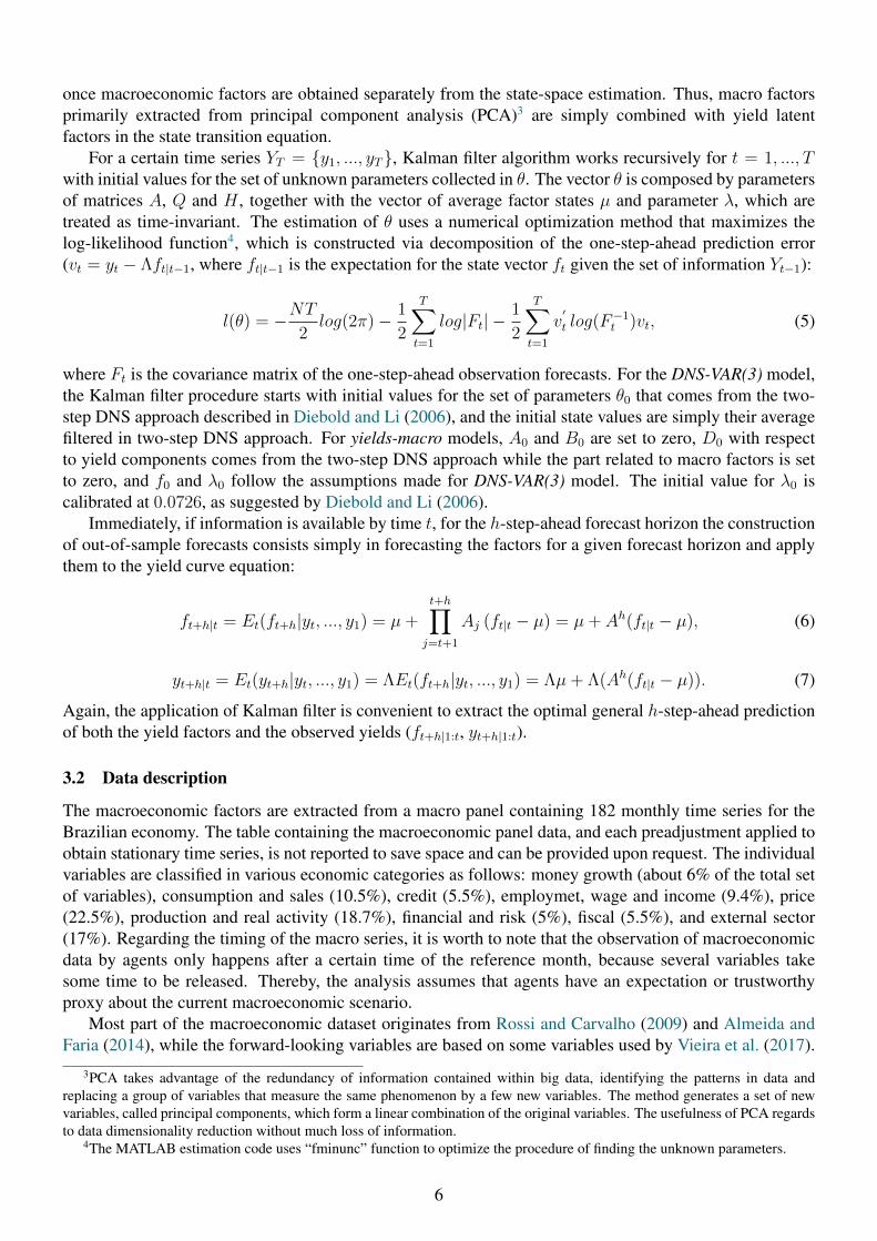
For a certain time series YT = y1, ..., yT, Kalman filter algorithm works recursively for t = 1, ..., Twith initial values for the set of unknown parameters collected in θ. The vector θ is composed by parametersof matrices A, Q and H , together with the vector of average factor states µ and parameter λ, which aretreated as time-invariant. The estimation of θ uses a numerical optimization method that maximizes thelog-likelihood function4, which is constructed via decomposition of the one-step-ahead prediction error(vt = yt − Λft|t−1, where ft|t−1 is the expectation for the state vector ft given the set of information Yt−1):

l(θ) = −NT2log(2π)− 1

2

T∑t=1

log|Ft| −1

2

T∑t=1

v′

t log(F−1t )vt, (5)

where Ft is the covariance matrix of the one-step-ahead observation forecasts. For the DNS-VAR(3) model,the Kalman filter procedure starts with initial values for the set of parameters θ0 that comes from the two-step DNS approach described in Diebold and Li (2006), and the initial state values are simply their averagefiltered in two-step DNS approach. For yields-macro models, A0 and B0 are set to zero, D0 with respectto yield components comes from the two-step DNS approach while the part related to macro factors is setto zero, and f0 and λ0 follow the assumptions made for DNS-VAR(3) model. The initial value for λ0 iscalibrated at 0.0726, as suggested by Diebold and Li (2006).

Immediately, if information is available by time t, for the h-step-ahead forecast horizon the constructionof out-of-sample forecasts consists simply in forecasting the factors for a given forecast horizon and applythem to the yield curve equation:

ft+h|t = Et(ft+h|yt, ..., y1) = µ+t+h∏j=t+1

Aj (ft|t − µ) = µ+ Ah(ft|t − µ), (6)

yt+h|t = Et(yt+h|yt, ..., y1) = ΛEt(ft+h|yt, ..., y1) = Λµ+ Λ(Ah(ft|t − µ)). (7)

Again, the application of Kalman filter is convenient to extract the optimal general h-step-ahead predictionof both the yield factors and the observed yields (ft+h|1:t, yt+h|1:t).

3.2 Data description

The macroeconomic factors are extracted from a macro panel containing 182 monthly time series for theBrazilian economy. The table containing the macroeconomic panel data, and each preadjustment applied toobtain stationary time series, is not reported to save space and can be provided upon request. The individualvariables are classified in various economic categories as follows: money growth (about 6% of the total setof variables), consumption and sales (10.5%), credit (5.5%), employmet, wage and income (9.4%), price(22.5%), production and real activity (18.7%), financial and risk (5%), fiscal (5.5%), and external sector(17%). Regarding the timing of the macro series, it is worth to note that the observation of macroeconomicdata by agents only happens after a certain time of the reference month, because several variables takesome time to be released. Thereby, the analysis assumes that agents have an expectation or trustworthyproxy about the current macroeconomic scenario.

Most part of the macroeconomic dataset originates from Rossi and Carvalho (2009) and Almeida andFaria (2014), while the forward-looking variables are based on some variables used by Vieira et al. (2017).

3PCA takes advantage of the redundancy of information contained within big data, identifying the patterns in data andreplacing a group of variables that measure the same phenomenon by a few new variables. The method generates a set of newvariables, called principal components, which form a linear combination of the original variables. The usefulness of PCA regardsto data dimensionality reduction without much loss of information.

4The MATLAB estimation code uses “fminunc” function to optimize the procedure of finding the unknown parameters.

6

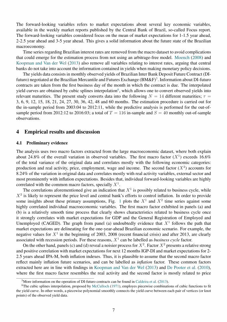
The forward-looking variables refers to market expectations about several key economic variables,available in the weekly market reports published by the Central Bank of Brazil, so-called Focus report.The forward-looking variables considered focus on the mean of market expectations for 1-1.5 year ahead,2-2.5 year ahead and 3-5 year ahead. This gives a solid information about the future state of the Brazilianmacroeconomy.

Time series regarding Brazilian interest rates are removed from the macro dataset to avoid complicationsthat could emerge for the estimation process from not using an arbitrage-free model. Moench (2008) andKoopman and Van der Wel (2013) also remove all variables relating to interest rates, arguing that centralbanks do not take into account the information contained in yields when making monetary policy decisions.

The yields data consists in monthly observed yields of Brazilian Inter Bank Deposit Future Contract (DI-futuro) negotiated at the Brazilian Mercantile and Futures Exchange (BM&F)5. Information about DI-futurocontracts are taken from the first business day of the month in which the contract is due. The interpolatedyield curves are obtained by cubic splines interpolation6, which allows one to convert observed yields intorelevant maturities. The present study converts data into the following N = 14 different maturities; τ =3, 6, 9, 12, 15, 18, 21, 24, 27, 30, 36, 42, 48 and 60 months. The estimation procedure is carried out forthe in-sample period from 2003:04 to 2012:11, while the predictive analysis is performed for the out-of-sample period from 2012:12 to 2016:03; a total of T = 116 in-sample and S = 40 monthly out-of-sampleobservations.

4 Empirical results and discussion

4.1 Preliminary evidence

The analysis uses two macro factors extracted from the large macroeconomic dataset, where both explainabout 24.8% of the overall variation in observed variables. The first macro factor (X1) exceeds 16.6%of the total variance of the original data and correlates mostly with the following economic categories:production and real activity, price, employment, wage and income. The second factor (X2) accounts for8.24% of the variation in original data and correlates mostly with real activity variables, external sector andmost prominently with inflation expectations. Besides that, individual forward-looking variables are highlycorrelated with the common macro factors, specially X1.

The correlations aforementioned give an indication that X1 is possibly related to business cycle, whileX2 is likely to represent the price level and central bank’s efforts to control inflation. In order to providesome insights about these primary assumptions, Fig. 1 plots the X1 and X2 time series against somehighly correlated individual macroeconomic variables. The first macro factor exhibited in panels (a) and(b) is a relatively smooth time process that clearly shows characteristics related to business cycle onceit strongly correlates with market expectations for GDP and the General Registration of Employed andUnemployed (CAGED). The graph from panel (a) undoubtedly evidence that X1 follows the path thatmarket expectations are delineating for the one-year-ahead Brazilian economic scenario. For example, thenegative values for X1 in the beginning of 2003, 2008 (recent financial crisis) and after 2013, are clearlyassociated with recession periods. For these reasons, X1 can be labelled as business cycle factor.

On the other hand, panels (c) and (d) reveal a noisier process forX2. FactorX2 presents a relative strongand positive correlation with market expectations for next 12 months IGP-DI and market expectations for 2-2.5 years ahead IPA-M, both inflation indexes. Thus, it is plausible to assume that the second macro factorreflect mainly inflation future scenarios, and can be labelled as inflation factor. These common factorsextracted here are in line with findings in Koopman and Van der Wel (2013) and De Pooter et al. (2010),where the first macro factor resembles the real activity and the second factor is mostly related to price

5More information on the operation of DI-futuro contracts can be found in Caldeira et al. (2013).6The cubic splines interpolation, proposed by McCulloch (1971), employes piecewise combinations of cubic functions to fit

the yield curve. In other words, a piecewise polynomial smoothly connects the yield curve between each pair of vertices (or knotpoints) of the observed yield data.

7

indexes.

(a) (b)

(c) (d)

Figure 1: Plots of common macro factors and individual most correlated macroeconomic variables.

Next, table 2 presents summary statistics for the yield dataset at some selected maturities, including theyield latent factors and the first two standardized macroeconomic factors, dividing between in-sample andout-of-sample periods. As analyzed in Diebold and Rudebusch (2013), several important yield curve factsemerge: (i) time-averaged yields increase with maturity revealing an increasing and slightly concave shape;which reports some kind of term premium, perhaps due to risk aversion, liquidity preferences, or preferredhabitats; (ii) yield volatilities decrease with maturity; (iii) yields are highly persistent, as evidenced bythe very large 1-month spread autocorrelations, specially for shorter maturities, and by the significant 12-month autocorrelations for the in-sample period. Despite being a period with increasingly shifts in yieldcurve levels, the out-of-sample period reports lower yield levels in comparison with the in-sample period,and thus, reduced volatility levels.

The in-sample observed yields data show an asymmetric distribution, where most of the observationsconcentrate in lower rates, while the out-of-sample yields data only show the same behavior for shortermaturities. In addition, the in-sample level factor is skewed to the right due to high observed yields ofthe first years of the sample period. The slope factor is negative in most part of both sample periods andconcentrate in the second quantile of its sample distribution. The observations regarding X1 pursue areaswith positive values, albeit having an absolute minimum value higher than its maximum. So, as X1 ishighly correlated with business cycle, its sample statistics reflect that there are more procyclical periods inthe Brazilian economy overall the sample period. The observations of X2 point to a sample distributionslightly skewed to the left, where data variation is larger for negative values. When it comes to sampleautocorrelations, the latent yield factors and X1 exhibit high persistences at displacement of 1 month, whileX2 shows a moderate persistence for the in-sample period.

8

Table 2: Summary statistics of yields and macro factors.

Mean SdQuantiles

ρ(1) ρ(12)Min Q(25%) Median Q(75%) Max

In-Sample Period Dataset: 2003:04 - 2012:11

DI-futuro yields (by maturity)

3 0.1356 0.0410 0.0741 0.1085 0.1233 0.1620 0.2617 0.9415 0.42579 0.1354 0.0381 0.0722 0.1097 0.1253 0.1603 0.2441 0.9388 0.4444

15 0.1369 0.0360 0.0745 0.1117 0.1268 0.1623 0.2429 0.9297 0.433327 0.1395 0.0337 0.0803 0.1164 0.1297 0.1659 0.2454 0.9136 0.444236 0.1406 0.0335 0.0827 0.1177 0.1293 0.1650 0.2516 0.9042 0.465660 0.1421 0.0345 0.0866 0.1199 0.1297 0.1639 0.2579 0.9041 0.4893

Yield curve latent factors (level, slope and curvature)

Lt 0.1459 0.0390 0.0948 0.1205 0.1328 0.1561 0.2913 0.8878 0.4746St -0.0139 0.0297 -0.0806 -0.0332 -0.0173 0.0005 0.0567 0.8831 -0.0377Ct -0.0029 0.0435 -0.1159 -0.0321 -0.0022 0.0287 0.1136 0.8951 0.0058

First two standardized principal components (PC) from the macro series

1st PC 0 1 -4.3332 -0.5690 0.1103 0.6944 1.6153 0.8249 0.18242st PC 0 1 -2.8687 -0.7395 -0.0199 0.5401 4.1118 0.4741 0.3055

Out-of-Sample Period Dataset: 2012:12 - 2016:03

DI-futuro yields (by maturity)

3 0.1140 0.0244 0.0703 0.1004 0.1113 0.1401 0.1474 0.9389 0.11299 0.1176 0.0240 0.0719 0.1031 0.1149 0.1386 0.1565 0.9260 0.1093

15 0.1197 0.0233 0.0734 0.1077 0.1192 0.1364 0.1613 0.9147 0.088127 0.1224 0.0214 0.0800 0.1131 0.1221 0.1329 0.1664 0.8985 0.036436 0.1231 0.0211 0.0819 0.1141 0.1230 0.1307 0.1671 0.8943 0.002460 0.1243 0.0196 0.0864 0.1173 0.1236 0.1292 0.1662 0.8858 -0.0687

Yield curve latent factors (level, slope and curvature)

Lt 0.1266 0.0198 0.0925 0.1173 0.1229 0.1346 0.1689 0.8658 -0.1762St -0.0144 0.0172 -0.0395 -0.0281 -0.0177 -0.0008 0.0269 0.8036 -0.0916Ct -0.0041 0.0282 -0.0606 -0.0243 -0.0073 0.0243 0.0539 0.6962 -0.0750

First two standardized principal components (PC) from the macro series

1st PC 0 1 -1.8151 -0.9609 0.2068 0.8576 1.6432 0.8406 0.12822st PC 0 1 -2.0911 -0.5877 0.0283 0.7151 2.0193 0.1160 -0.0394

Notes: The table presents the descriptive statistics for DI-futuro contracts over the in-sample and out-of-sample periods. The monthly yield curves were constructed using cubic splines interpolation. For eachmaturity, the table displays the mean, standard deviation (Sd), minimum (Min), 25% quantile, median, 75%quantile, maximum (Max), and sample autocorrelations at displacements of 1 (ρ(1)) and 12 (ρ(12)) months.In addition, it shows the statistics for the yield latent factors and for the first two standardized principalcomponents extracted from the macro dataset.

4.2 Estimating term structure models

In-sample estimates

The results obtained from estimating the DNS specification models represented by DNS-VAR(3) and theset of yields-macro models, defined in Section 2, indicate that on average the estimated models providea good fit to the yield curve across the entire maturity spectrum, except for very short maturities. Formaturities above 9 months the models fit the observed data efficiently well. The bad fit behavior for shortmaturities also is reported by Diebold et al. (2006), where estimated errors for yields of 3-months maturityare relatively higher. In addition, yield curve estimates of the macroeconomic specifications for mediumand long-term maturities are more accurate than DNS-VAR(3) estimates. Furthermore, the estimated errorsof DNS-VAR(5) model are higher compared to DNS-VAR(4)2 model. These results sign for a path wheremacroeconomic information can improve yield curve predictions, at least for longer maturities.

9

Out-of-sample estimates

In this section, we perform the out-of-sample forecast exercise using a rolling window analysis. Thisimplies that the multiple step ahead forecasts explored here are closely related to an investor’s pseudoreal-time decision. However, the analysis is not based on fully real-time data once some macroeconomicvariables are constructed from the revised dataset and some macro information have not been released yetat the time when a forecast is made.

The forecast exercise for the multiple forecast horizons of 1-, 3-, 6-, 9- and 12-month-ahead areperformed with rolling window samples of size T = 116. Hence, the out-of-sample forecasts are carriedout over the time interval from December 2012, to March 2016. Predictions are made for T + h at the endof each rolling window, where h is the forecast horizon. The number of rolling window samples is S = 40,whereas the last 11 rolling window samples have some restrictions related to forecast horizons. That is,there are 40 out-of-sample forecasts for 1-month horizon, 39 for 2-month horizon, and so on until 29out-of-sample forecasts for 12-month horizon.

The evaluation of out-of-sample forecasts requires some measures to compute the errors for eachmaturity τi. Given a time series of S out-of-sample forecasts for h-period-ahead forecast horizon, the rootmean squared forecast error (RMSFE) calculates a forecast error measure for maturity τi at forecasthorizon h and for model m:

RMSFEm(τi) =

√√√√ 1

S

S∑t=1

(yt+h|t(τi)− yt+h(τi))2, (8)

where yt+h(τi) is the yield for the maturity τi observed at time t + h, and yt+h|t(τi) is the correspondingforecast made at time t. The performance analysis also reports the trace root mean squared forecast error(TRMSFE), which calculates the trace of the covariance matrix of the forecast errors across allN maturities:

TRMSFEm(τi) =

√√√√ 1

N

1

S

N∑i=1

S∑t=1

(yt+h|t(τi)− yt+h(τi))2 (9)

The Giacomini and White (2006) test is applied to compare forecast accuracy between two competingmodels. The Giacomini-White (GW) statistic is a test of conditional forecasting ability, handling forecastsbased on both nested and non-nested models, and is constructed under the assumption that forecasts aregenerated using a moving data window. In this case, the GW test evaluates whether the out-of-sampleforecast error from the random walk (RW) model for maturity τi (eRWt+h|t(τi)) is statistically different fromthe forecasts of the competing DNS model. The test is based on the loss differential function dm,t =(eRWt+h|t(τi))

2 − (eDNSt+h|t(τi))2. Thus, we assume a quadratic loss function, where the null hypothesis of equal

forecasting accuracy can be written as

H0 : E[dm,t+h|δm,t] = 0. (10)

Parameter δm,t is a p×1 vector of test functions. The GW test statistic GWm,t can be computed as the Waldstatistic:

GWm,t = S

(S−1

S−h∑t=T+1

δm,tdm,t+h

)′Ω−1S

(S−1

S−h∑t=T+1

δm,tdm,t+h

)d→ χ2

dim(δ), (11)

where Ω−1S is a consistent HAC estimator for the asymptotic variance of δm,tdm,t+h, and S the number ofout-of-sample observations. Under the null hypothesis given in 10, the test statistic GWi,t is asymptoticallydistributed as χ2

p.Table 3 reports the summary statistics of forecast performance for the general specifications: DNS-

VAR(3), DNS-VAR(4) and DNS-VAR(5). The following basic considerations can be made: (i) the DNS-

10

Table 3: (Trace)-Root Mean Squared Forecast Errors of DNS-VAR(3) and yields-macro models.

Panel A: DNS-VAR(3) model Panel B: DNS-VAR(5) model

MaturitiesForecast horizon Forecast horizon

1-M 3-M 6-M 9-M 12-M 1-M 3-M 6-M 9-M 12-M

3 0.486∗ 0.969∗ 1.817 2.472 2.978 1.424 2.422 3.357 6.536 14.2046 0.478∗ 0.987 1.761 2.313 2.739 1.491 2.435 3.275 6.217 13.395∗

9 0.502∗ 1.021 1.691 2.185 2.581∗ 1.565 2.487 3.211 5.936 12.710∗

12 0.536 1.043 1.641 2.112 2.468∗ 1.622 2.508 3.166 5.705 12.141∗

15 0.546∗ 1.049 1.610 2.058∗ 2.381∗ 1.654 2.530 3.112 5.482 11.585∗

18 0.574∗ 1.084∗ 1.620 2.033∗ 2.329∗ 1.687 2.542 3.048 5.239 11.063∗

21 0.600∗ 1.114 1.628 2.020∗ 2.287∗ 1.708 2.537 2.985 5.009 10.565∗

24 0.615∗ 1.125 1.643 2.020∗ 2.264∗ 1.717 2.527 2.942 4.805 10.090∗

27 0.617∗ 1.132 1.654 2.005∗ 2.250∗ 1.718 2.519 2.912 4.608 9.640∗

30 0.622∗ 1.139 1.652 1.994∗ 2.241∗ 1.722 2.511 2.891 4.422 9.212∗

36 0.624∗ 1.134 1.658 2.001∗ 2.242∗ 1.728 2.511 2.838 4.112 8.452∗

42 0.630∗ 1.138 1.675 2.012∗ 2.257∗ 1.726 2.507 2.818 3.880 7.811∗

48 0.633∗ 1.132 1.670 2.012∗ 2.262∗ 1.717 2.510 2.816 3.699 7.292∗

60 0.640∗ 1.125 1.670 2.023∗ 2.267∗ 1.727 2.550 2.869 3.519 6.624∗

TRMSFE 0.581 1.087 1.672 2.094 2.406 1.660 2.507 3.022 5.026 10.581

Panel C: DNS-VAR(4)1 model Panel D: DNS-VAR(4)2 model

MaturitiesForecast horizon Forecast horizon

1-M 3-M 6-M 9-M 12-M 1-M 3-M 6-M 9-M 12-M

3 1.864 2.925 4.304 5.949∗ 8.216∗ 0.523∗ 1.069 1.724∗ 2.202 2.483∗6 1.834∗ 2.936 4.251∗ 5.823∗ 7.924∗ 0.520∗ 1.044 1.638 2.015 2.2859 1.793∗ 2.920∗ 4.185∗ 5.706∗ 7.688∗ 0.556 1.043 1.560 1.894 2.121

12 1.773∗ 2.908∗ 4.103∗ 5.595∗ 7.430∗ 0.592 1.051 1.520 1.798 2.010∗15 1.738∗ 2.873∗ 4.020∗ 5.454∗ 7.215∗ 0.616∗ 1.049∗ 1.484 1.731∗ 1.912∗18 1.714∗ 2.848∗ 3.929∗ 5.323∗ 7.001∗ 0.645∗ 1.067∗ 1.484 1.695∗ 1.841∗21 1.687∗ 2.803∗ 3.853∗ 5.206∗ 6.793∗ 0.665∗ 1.090∗ 1.489 1.669∗ 1.787∗24 1.661∗ 2.763∗ 3.784∗ 5.087∗ 6.614∗ 0.677∗ 1.095∗ 1.495∗ 1.647∗ 1.760∗27 1.638∗ 2.725∗ 3.697∗ 4.979∗ 6.459∗ 0.680∗ 1.102 1.497∗ 1.641∗ 1.757∗30 1.612∗ 2.694∗ 3.607∗ 4.884∗ 6.322∗ 0.687∗ 1.106∗ 1.502∗ 1.636∗ 1.756∗36 1.594 2.617∗ 3.511∗ 4.712∗ 6.077∗ 0.703∗ 1.121 1.510∗ 1.639∗ 1.765∗42 1.571 2.564∗ 3.429∗ 4.572∗ 5.889∗ 0.709∗ 1.125 1.520∗ 1.657∗ 1.786∗48 1.548 2.510∗ 3.347∗ 4.455∗ 5.724∗ 0.711∗ 1.122 1.515∗ 1.661∗ 1.797∗60 1.518 2.431∗ 3.228 4.275∗ 5.468∗ 0.715∗ 1.121 1.516∗ 1.677∗ 1.813∗

TRMSFE 1.685 2.756 3.818 5.169 6.822 0.646 1.086 1.534 1.762 1.932

Notes: The table presents the forecasting performances of DNS-VAR(3) model and yields-macro models. Inparticular, it reports the RMSFE and TRMSFE statistics obtained by using individual DNS-VAR(3), DNS-VAR(4)1,DNS-VAR(4)2 and DNS-VAR(5) models. The values reported are divided by 1 × 10−2. The RMSFE is reported foreach model for the τ maturities and for 1-, 3-, 6-, 9- and 12-month-ahead forecast horizons. The latest line of eachpanel reports the TRMSFE for the different forecast horizons. Numbers in bold indicate that the alternative yields-macro models from panels B, C and D outperform the DNS-VAR(3) model, otherwise indicate underperformance.Number in italic indicate that the DNS model outperform the random walk model. The star on the right of the cellentries indicate where the GW test rejects the null of equal forecasting accuracy between the competitor yields-macromodels and random walk, with 10% probability of the null hypothesis.

VAR(5) and DNS-VAR(4)1 clearly underperform the general DNS framework for the entire maturity andforecast horizon spectrum; (ii) the DNS-VAR(4)2 consistently outperform the DNS-VAR(3) model for mostmaturities and for forecast horizons longer than one month. The GW test rejects the null hypothesis at a 10%level of the DNS-VAR(4)2 model for some particular cases: (i) 3-month-ahead predictions at medium-termmaturities; (ii) 6-month-ahead predictions for maturities above 24 months; and (ii) 9- and 12-month-aheadpredictions for the medium and long end of the yield curve. Therefore, the DNS-VAR(4)2 model generatesbetter forecasts for forecast horizons longer than one month at medium- and long-term maturities.

The GW test also rejects the null for most forecasted yields of DNS-VAR(4)1 model and few 12-month-ahead forecasted yields of the DNS-VAR(5) model, confirming their inferior performance in relation to theRW and DNS-VAR(3) models. Both specifications which include the business cycle factor forecast poorly,supporting the evidence of relatively small impact of X1 on the Brazilian yield curve. In other words,

11

the incorporation of macro factors containing information strongly correlated with business cycle do notcontribute to predict the Brazilian yield curve.

The forecasts produced by the DNS-VAR(4)2 model provide the lowest RMSFEs and TRMSFEs formost predictions above 1-month horizon, while DNS-VAR(3) and RW provide the lowest values for1-month-ahead forecasts. Thus, the inclusion of the inflation factor into the general DNS frameworkappears to lead to lower RMSFEs for most interest rates and most forecast horizons above 1 month, whereresults for the GW tests indicate significant improvements from forecasting with DNS-VAR(4)2 in relationto RW. Overall, the results imply the support for the incorporation of a macro factor that summarizes broadmacroeconomic information regarding mainly inflation expectations. The forecast exercise confirms theestimates reported by Moench (2008), De Pooter et al. (2010), Koopman and Van der Wel (2013), Almeidaand Faria (2014), among other studies which report better out-of-sample yield forecasts for term structuremodels with macroeconomic appeal.

4.3 Application to fixed-income portfolio optimization

The mean-variance portfolio problem

The approach suggested by Markowitz (1952) is the most common formulation of portfolio choiceproblems, which point out that investors allocate their wealth in risky assets based on the trade-off betweenexpected return and risk. At the moment of the portfolio choice, it is assumed that investors are onlyconcerned with the expected returns for the h-step-ahead forecast horizon and its covariance matrix,defined by µrt|t−h

and Σrt|t−h, respectively. The mean-variance portfolio problem can then be formulated

by minimizing the portfolio variance for a particular h-step-ahead expected return, subject to additionalrestrictions on the vector of optimal weights wt:

Minwt

w′

t Σrt|t−hwt −

1

δw′

t µrt|t−h

subject to : w′

tı = 1; wt ≥ 0. (12)

where ı is an appropriately sized vector of ones and δ is the investor’s risk aversion coefficient. Vectorµrt|t−h

collects the h-step-ahead expected returns for maturities τ1, ..., τN , so that its dimension is N × 1,while the covariance matrix Σrt|t−h

is N × N . The optimization problem is subject to both constraints,the non-negative individual weights, which restricts short sales, and the budget constraint, which ensuresthat all wealth is invested in risky assets. As the mean-variance problem solves a quadratic utility function,the necessary and sufficient condition for optimization is to solve the optimal weights wt for the first ordercondition.

The distribution of log-returns

Following the discussion in Caldeira et al. (2016), factor models for the term structure of interest rates aredesigned only to model bond yields. Thus, the forecasting stage of yield curve models aim for modelingmerely moments of the expected yields. However, the fixed-income portfolio problem requires estimatesof the expected return of each maturity, as well as estimates of their covariance matrix. The followingmathematical decompositions show that it is possible to obtain expressions for the expected return of fixed-income securities and their covariance matrix based on the distribution of the expected yields.

The mean-variance portfolio optimization is performed for two different forecast horizons: (i) first, one-step-ahead forecasts for log-returns of DI-futuro contracts are used to optimize fixed-income portfolios withmonthly rebalancing; and subsequently (ii) six-step-ahead forecasts for log-returns are used to find optimalportfolios with biannual rebalancing. For this reason, the portfolio choice problem requires moments of theexpected yields for one- and six-months-ahead forecast horizons. The system of Eqs. (2)-(4) impliesthat the distribution of one-step-ahead forecasts for yt, of any maturity τi, is normally distributed, i.e.

12

yt|t−1 ∼ N(µyt|t−1,Σyt|t−1

), with moments given by7:

µyt|t−1= Et−1[yt] = Λft|t−1, (13)

andΣyt|t−1

= Λ(APt−1|t−1A′ +Q)Λ′ +H, (14)

where Pt|t denotes the filtered covariance matrix of ft|t at time t. Eq. (13) follows straightforward from Eq.(7), which define the expectation of yields for the h-step-ahead forecast horizon. Note that the covariancematrix of the true, but non-observable states (ft), would be given simply by Q. However, as stated in Eq.(13), predicted states based on filtered estimates of ft−1 are used when computing expected yields. Thus,Eq. (14) takes into account the uncertainty in the Kalman filter estimates of the unobserved factors throughAPt−1|t−1A

′, containing the covariance matrix of the filtered states (Pt−1|t−1) and not only the covariancematrix of the unobserved factors, Q8. Therefore, the first term in Eq. (14), APt−1|t−1A′+Q, adjusts for thefact that filtered estimates are used in (13), and not the true value of states.

Similarly, the distribution of six-step-ahead forecasts, yt|t−6 ∼ N(µyt|t−6,Σyt|t−6

), is normallydistributed with moments given by:

µyt|t−6= Et−6[yt] = Λft|t−6, (15)

and

Σyt|t−6= Λ(A6Pt−6|t−6A

′ 6 +6∑i=1

Ai−1QA′ i−1)Λ′ +H. (16)

Note that, in this case, the term (A6Pt−6|t−6A′ 6+

∑6i=1A

i−1QA′ i−1) adjusts for the fact that the model usesfiltered estimates for the six-step-ahead forecasts of yields and accumulates the uncertainty in the Kalmanfilter estimates for each step forecast.

Using the mathematical expression for the discount curve Pt(τi) = exp(−τi · yt(τi)) and the log-returnexpression, the realized return, rt(τi), of holding a security from t−h to t while its maturity decreases fromτi to τi−h, can be computed as follows,

rt(τi) = log(Pt(τi−h)

Pt−h(τi)

)= logPt(τi−h)− logPt−h(τi) = −τi−h · yt(τi−h) + τi · yt−h(τi). (17)

It is clear to note from (13)-(17) that the vector of h-step-ahead forecasts of log-returns, rt|t−h, also followsa Normal distribution N(µrt|t−h

,Σrt|t−h) with mean given by:

µrt|t−h= −τi−h ⊗ µyt|t−h

(τi−h) + τi ⊗ yt−h|t−h(τi), (18)

where µyt|t−h(τi−h) is the mean vector of the expected yields with maturity τi−h at time t conditional on

period t− h information, yt−h|t−h(τi) is the vector of observed yields with maturity τi at time t− h, and ⊗represents the Hadamard (elementwise) multiplication. The conditional covariance matrix of the expectedlog-returns, which is positive-definite, is given by:

Σrt|t−h= τ ′i−hτi−h ⊗ Σyt|t−h

. (19)

The discussion above solves the problem for obtaining estimates of the expected log-returns forfixed-income securities and their covariance matrix based on yield curve models such as the DNS model,which are essential inputs to the portfolio choice problem based on the mean-variance approach suggested

7(Durbin and Koopman, 2012, p. 112) define the general formulations for the conditional mean square error matrix andconditional mean of the covariance matrix of predicted states.

8For comparison, Caldeira et al. (2013) use the true value of the state vector and show that the second moment of yt|t−1 justtakes into account the covariance matrix of the unobserved factors, Q.

13

by Markowitz. All ingredients necessary to calculating the closed-form expressions (18)-(19) are easilyretrieved from the Kalman filter estimation discussed in Section 3.

Methodology for evaluating portfolio performance and implementation details

This section aims to assess the economic value of the forecasting ability of the major yield curve modelsestimated previously. The empirical implementation of the mean-variance optimization problem definedby (12) is performed by using one- and six-step-ahead estimates of the vector of expected returns andits covariance matrix considering five alternative values for the risk aversion coefficient δ: 0.0001, 0.01,0.1, 0.5 and 1. Following the recursive estimation strategy of the yield curve models, the optimal mean-variance portfolios are also computed recursively as new h-step-ahead estimates for DI-futuro returns areknown. Moreover, optimal mean-variance portfolios using one-step-ahead forecasts for DI-futuro returnsare rebalanced on a monthly basis, while portfolios using six-step-ahead forecasts are rebalanced on abiannual basis. Thus, the empirical analysis with monthly rebalancing computes the optimal portfolio foreach period over the S out-of-sample observations giving a sample of 40 optimal portfolio weights wt.

Otherwise, the optimization with biannual rebalancing computes the optimal portfolio each sixconsecutive months. Nevertheless, the portfolio performance statistics are computed for every month ofthe out-of-sample period. The last rebalancing procedure is performed at May 2015, because as fromSeptember 2015, there are no forecasts for 6-month-ahead yields being considered by the yield curvemodels. Moreover, rebalancing frequency is important when dealing with fixed-income assets, because thesecurities in the portfolio can age and be closer to maturity. For this reason, the shortest maturityconsidered here is τi = 9 months, because DI-futuro contracts with maturity lower or equal to 6 monthswill already be matured before the subsequent rebalancing process. This only allows the computation ofperformance statistics until January 2016, because at February 2016 the 9-month security will already bematured, so that the number of out-of-sample observations is equal to 38.

It is clear that the scenario with biannual rebalancing requires more diligence regarding implementationprocedure and computation of performance statistics. Note that, after one period, an optimal portfoliocontaining securities that yield an average duration of τi at the time of the mean-variance optimization,becomes a portfolio with average duration τi−1 and so on until the next rebalancing process, changing thecharacteristics of the original portfolio over time. Thus, the computation of the time series of portfolioreturns need to take care about the constant decrease of the time-to-maturity of its securities.

The performance analysis use some alternative criteria to evaluate the performance of the optimal mean-variance fixed-income portfolios. First of all, we describe the evaluation criteria related to portfolio excessreturn relative to the risk-free rate (Rft), which is consider to be the short Brazilian Interbank Deposit(CDI) rate. The average gross (i.e., before transaction costs) excess return relative to the risk-free rate (rx)is calculated as follows:

rx =1

S

S∑t=1

rxt,

where rxt = w′t−1Rt − Rft denotes the gross excess portfolio return at time t and Rt = [rt(τi), ..., rt(τN)]′

is a vector collecting DI-futuro returns of all maturities considered.According to Han (2006), it would be appropriate to consider transaction costs when rebalancing the

portfolio weights frequently. The empirical scenario with biannual rebalancing can alleviate the impact oftransaction costs on portfolio performance. However, the less frequent rebalancing means that the portfolioweights will be outdated, which could negatively affect the portfolio performance because investors wouldbe investing away from the optimal one (Caldeira et al., 2016). The performance analysis also considers theexcess return net of transaction costs (rxnett ), which takes into account the negative impact of transactioncosts on portfolio average performance, and is calculated as:

rxnett = (1− c · turnovert)(1 + rxt)− 1, (20)

14

where c is the fee that must be paid for each transaction and turnovert is the portfolio turnover at time t,defined as the fraction of wealth traded between periods t− 1 and t, i.e,

turnovert =N∑i=1

(|wi,t − wi,t−1|).

The parameter wi,t is the optimal weight of maturity τi at time t. The level of transaction costs beingconsidered is 5 bps, reflecting a fixed percentage for each rebalance trade. Similarly to rx, the averageexcess portfolio return net of transaction costs is defined as rxnet = 1

S

∑St=1 rx

nett . Moreover, statistics

regarding the volatility (standard deviation) of the net excess return (σ) and the risk-adjusted net excessreturn (SR) measured by the Sharpe ratio are calculated as follows,

σ =

√√√√ 1

S

S∑t=1

(rxnett − µp)2,

SR =rxnet

σ,

where µp denotes the sample mean of the portfolio net excess return. Ultimately, the performance analysistakes into account the average duration in years of the portfolios, which allows one to better understandthe composition of the optimal portfolios. The average duration of a fixed-income portfolio is calculated as1S

∑St=1w

′tτ , where here τ regards to the vector of individual security durations. A higher (lower) average

portfolio duration suggests that the optimal portfolio is invested in long (short) maturities.

Results for mean-variance portfolios

Table 4 reports the out-of-sample performance of mean-variance portfolios of DI-futuro contracts that useestimates of yields from the random walk (RW)9, DNS-VAR(3) and DNS-VAR(4)2 model specifications. Forthe scenario which considers one-step-ahead estimates and more frequent portfolio rebalancing (Panel Ain Table 4), the overview indicates that positive excess return statistics are essentially obtained when therisk aversion coefficient is higher than 0.01, where the annualized net excess returns range from 0.40% to1.57%. The best overall performance in terms of Sharpe ratio is achieved by the mean-variance portfolioobtained with the RW model with δ = 0.5 (SR = 0.472). When lower risk aversion is considered, most ofthe results indicate negative Sharpe ratios and higher volatility levels. As expected, an increase in the riskaversion coefficient leads to decreases in portfolio volatility as well as decreases in the average duration,that is, optimal portfolios are invested in short-term maturities. This result is intuitive since lower maturitysecurities are less risky, allowing investors with higher risk aversion to lower portfolio risk by investingin shorter maturities. This evidence is even more pronounced for the RW model, which quickly decreasesvolatility and duration with the increase of δ, investing basically in 3- and 6-month maturities for δ’s higherthan 0.1. For instance, the average portfolio duration across specifications for an investor with risk aversioncoefficient δ = 1 is 0.89 year, whereas the same indicator for an investor with δ = 1× 10−4 is 2.37 years.

On the other hand, the scenario which considers six-step-ahead estimates for DI-futuro returns and abiannual portfolio rebalancing (Panel B in Table 4) reports negative net excess returns across all modelspecifications and across all levels of the risk tolerance considered, except for the DNS-VAR(4)2 model withδ < 1. The best overall performance are achieved by the DNS-VAR(4)2 model for the smallest δ: rx equal to1.075%, rxnet =1.065%, volatility (measured by the standard deviation) equal to 10.75%, SR = 0.099 andaverage duration equal to 1.55 years. The DNS-VAR(4)2 model also minimizes losses for the higher levelof δ. The general results show that annualized net excess returns range from -3.153% to 1.065%, and the

9It is noteworthy that the covariance matrix of the expected log-returns obtained from forecasted yields of the RW model issimply the sample covariance from the in-sample observations.

15

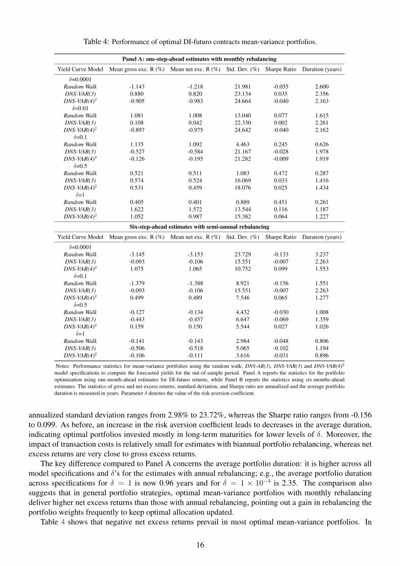
Table 4: Performance of optimal DI-futuro contracts mean-variance portfolios.

Panel A: one-step-ahead estimates with monthly rebalancing

Yield Curve Model Mean gross exc. R (%) Mean net exc. R (%) Std. Dev. (%) Sharpe Ratio Duration (years)

δ=0.0001Random Walk -1.143 -1.218 21.981 -0.055 2.600DNS-VAR(3) 0.880 0.820 23.134 0.035 2.356DNS-VAR(4)2 -0.905 -0.983 24.664 -0.040 2.163

δ=0.01Random Walk 1.081 1.008 13.040 0.077 1.615DNS-VAR(3) 0.108 0.042 22.330 0.002 2.261DNS-VAR(4)2 -0.897 -0.975 24.642 -0.040 2.162

δ=0.1Random Walk 1.135 1.092 4.463 0.245 0.626DNS-VAR(3) -0.527 -0.584 21.167 -0.028 1.978DNS-VAR(4)2 -0.126 -0.195 21.282 -0.009 1.919

δ=0.5Random Walk 0.521 0.511 1.083 0.472 0.287DNS-VAR(3) 0.574 0.524 16.069 0.033 1.416DNS-VAR(4)2 0.531 0.459 18.076 0.025 1.434

δ=1Random Walk 0.405 0.401 0.889 0.451 0.261DNS-VAR(3) 1.622 1.572 13.544 0.116 1.187DNS-VAR(4)2 1.052 0.987 15.382 0.064 1.227

Six-step-ahead estimates with semi-annual rebalancing

Yield Curve Model Mean gross exc. R (%) Mean net exc. R (%) Std. Dev. (%) Sharpe Ratio Duration (years)

δ=0.0001Random Walk -3.145 -3.153 23.729 -0.133 3.237DNS-VAR(3) -0.093 -0.106 15.551 -0.007 2.263DNS-VAR(4)2 1.075 1.065 10.752 0.099 1.553



δ=1Random Walk -0.141 -0.143 2.984 -0.048 0.806DNS-VAR(3) -0.506 -0.518 5.065 -0.102 1.194DNS-VAR(4)2 -0.106 -0.111 3.616 -0.031 0.896

Notes: Performance statistics for mean-variance portfolios using the random walk, DNS-AR(3), DNS-VAR(3) and DNS-VAR(4)2

model specifications to compute the forecasted yields for the out-of-sample period. Panel A reports the statistics for the portfoliooptimization using one-month-ahead estimates for DI-futuro returns, while Panel B reports the statistics using six-months-aheadestimates. The statistics of gross and net excess returns, standard deviation, and Sharpe ratio are annualized and the average portfolioduration is measured in years. Parameter δ denotes the value of the risk aversion coefficient.

annualized standard deviation ranges from 2.98% to 23.72%, whereas the Sharpe ratio ranges from -0.156to 0.099. As before, an increase in the risk aversion coefficient leads to decreases in the average duration,indicating optimal portfolios invested mostly in long-term maturities for lower levels of δ. Moreover, theimpact of transaction costs is relatively small for estimates with biannual portfolio rebalancing, whereas netexcess returns are very close to gross excess returns.

The key difference compared to Panel A concerns the average portfolio duration: it is higher across allmodel specifications and δ’s for the estimates with annual rebalancing; e.g., the average portfolio durationacross specifications for δ = 1 is now 0.96 years and for δ = 1 × 10−4 is 2.35. The comparison alsosuggests that in general portfolio strategies, optimal mean-variance portfolios with monthly rebalancingdeliver higher net excess returns than those with annual rebalancing, pointing out a gain in rebalancing theportfolio weights frequently to keep optimal allocation updated.

Table 4 shows that negative net excess returns prevail in most optimal mean-variance portfolios. In

16

rising interest rate environments, as the out-of-sample period, fixed-income prices suffer from the increasein interest rates in the short term, i.e, rising rate environments can result in negative fixed-income returns.A bond’s total return comprises not just price changes, but also income, so that the income on a bondcan help offset falling prices, cushioning the overall total return. It turns out that optimal mean-varianceportfolios can not benefit from increased yields over the long term because of rebalancing: investors do nothold fixed-income securities until their maturity, which turns portfolio’s total returns highly dependent onprice changes. For this reason, the income returns are not enough to offset the price decline in DI-futurocontracts.

At least, Fig. 2 illustrates the performance of the optimal DI-futuro mean-variance portfolios by plottingthe cumulative net returns over the out-of-sample period obtained with the alternative specifications whenδ is equal to 1 × 10−4 and 1. The figure suggests that DNS-VAR(3) delivers better performance for mean-variance portfolios using one-step-ahead estimates for returns and for δ = 1 × 10−4 during most part ofthe out-of-sample period. For δ = 1, the RW model reports more stable and higher cumulative returns.However, DNS-VAR(4)2 displays better portfolio performance using six-step-ahead estimates. The bestoverall performance in terms of cumulative net returns are achieved by mean-variance portfolios obtainedwith the RW model for δ = 1 and for one-step-ahead estimates (33.17%) and with the DNS-VAR(4)2

for δ = 1 × 10−4 and six-step-ahead estimates (33.85%). Hence, the incorporation of macroeconomicinformation has positive effects to achieve better portfolio performance at the biannual rebalancing scenario.

(a) (b)

(c) (d)

Figure 2: Cumulative net returns (in %): mean-variance portfolios with δ = 1 × 10−4 and δ = 1 for 1- and 6-step-ahead forecasts over the out-of-sample period.

It is also noteworthy the big drop in cumulative net returns for the one-step-ahead estimates inSeptember 2015. At the end of August 2015, there is a deterioration of the Brazilian macroeconomicfundamentals due to the perception of a downturn in medium- and long-term fiscal scenario. Financialmarkets reacted with capital flight to safer investments and investors required higher premiums for holdingBrazilian securities. Fig. 3 helps to visualize the scenario where short DI-futuro yields slightly rise whilelong-term yields suffer a large increase from July 2015, to September 2015, reflecting a large deteriorationin long-term expectations about Brazilian macroeconomic foundations. Once investors with more

17

risk-averse preferences tend to hold short-term maturities, they are not affected so much as the lessrisk-averse investors with δ = 1× 10−4 evidenced by panel (a) of Fig. 2.

Figure 3: Observed yield curves from July 2015, to September 2015.

The link between Tables 3 and 4 is clear in the sense that better accuracy in yield curve forecastingleads to an improvement in terms of portfolio performance based on the mean-variance approach. In thegeneral context, preferred one-month-ahead forecasted yields, which are generated by RW andDNS-VAR(3), deliver better portfolio performance for optimizations with one-step-ahead estimates forDI-futuro returns. On the other hand, the DNS-VAR(4)2 specification, which consistently outperforms itscompetitors for forecast horizons longer than one month, reports better portfolio performance usingsix-step-ahead estimates. It is noteworthy that these findings highlight the relevance of good yield curvepredictions to achieve better results in terms of portfolio performance. From this perspective, theincorporation of macroeconomic information into term structure models can play an important role toimprove performance of fixed-income portfolios with biannual rebalancing.

5 Concluding remarks

The recent literature on yield curve forecasting suggests that the incorporation of a large macroeconomicdataset into term structure models improve forecast accuracy (De Pooter et al., 2010). Most of currentstudies test for statistical benefits from incorporating macroeconomic information, but little is known aboutthe economic value of those forecasted yields. Besides testing for statistical improvement, this study usesa fixed-income portfolio analysis in order to assess the economic value of forecasted yields generated byyield curve models with macro factors extracted from a large macroeconomic dataset.

The out-of-sample forecast exercise support the evidence that a DNS yield curve model incorporatingone macro factor, which summarizes broad information regarding primarily inflation expectations,outperforms the general DNS and RW models for forecast horizons longer than one month, specially atmedium- and long-term maturities. This evidence indicates that an inflation factor is particularly useful topredict the Brazilian nominal yield curve dynamics.

The results for mean-variance portfolios show that better accuracy in yield curve forecasting leads toan improvement in terms of portfolio performance. Portfolio optimizations with six-step-ahead estimatesfor DI-futuro returns and biannual rebalancing report positive excess returns only for the DNS modelwhich incorporates the inflation factor. Moreover, optimal portfolios with monthly rebalancing deliverhigher return statistics for the general DNS model and RW, which forecasted yields outperform for theshort forecast horizon scenario.

The overview indicates that good yield curve predictions are important to achieve economic gains fromforecasted yields in terms of portfolio performance. It is clear that yield curve models with better forecastaccuracy for short forecast horizons perform quite well for optimal mean-variance portfolios with one-step-ahead estimates for DI-futuro returns. In parallel, the DNS specification which incorporates an inflationfactor outperforms in terms of portfolio performance with six-step-ahead estimates. Therefore, there isan economic and statistical gain from considering a large macroeconomic dataset to forecast the Brazilianyield curve dynamics, specially for longer forecast horizons.

18

References

Almeida, C. and A. Faria (2014). Forecasting the Brazilian term structure using macroeconomic factors.Brazilian Review of Econometrics 34(1), 45–77.

Ang, A. and M. Piazzesi (2003). A no-arbitrage vector autoregression of term structure dynamics withmacroeconomic and latent variables. Journal of Monetary economics 50(4), 745–787.

Bernanke, B. S. and J. Boivin (2003). Monetary policy in a data-rich environment. Journal of MonetaryEconomics 50(3), 525–546.

Bernanke, B. S., J. Boivin, and P. Eliasz (2005). Measuring the effects of monetary policy: A factor-augmented vector autoregressive (FAVAR) approach. The Quarterly Journal of Economics 120(1), 387–422.

Bolder, D. J. (2015). Fixed-Income Portfolio Analytics: A Practical Guide to Implementing, Monitoringand Understanding Fixed-Income Portfolios. Springer.

Caldeira, J. F., G. V. Moura, and A. A. P. Santos (2013). Measuring risk in fixed income portfolios usingyield curve models. Computational Economics 46(1), 65–82.

Caldeira, J. F., G. V. Moura, and A. A. P. Santos (2016). Bond portfolio optimization using dynamic factormodels. Journal of Empirical Finance 37, 128–158.

Caldeira, J. F., G. V. Moura, and M. Savino Portugal (2010). Efficient yield curve estimation and forecastingin brazil. Revista Economia, January/April.

Dai, Q. and K. J. Singleton (2000). Specification analysis of affine term structure models. The Journal ofFinance 55(5), 1943–1978.

De Pooter, M., F. Ravazzolo, and D. J. Van Dijk (2010). Term structure forecasting using macro factors andforecast combination. FRB International Finance Discussion Paper (993).

Diebold, F. X. and C. Li (2006). Forecasting the term structure of government bond yields. Journal ofEconometrics 130(2), 337–364.

Diebold, F. X. and G. D. Rudebusch (2013). Yield Curve Modeling and Forecasting: The Dynamic Nelson-Siegel Approach. Princeton University Press.

Diebold, F. X., G. D. Rudebusch, and S. B. Aruoba (2006). The macroeconomy and the yield curve: adynamic latent factor approach. Journal of Econometrics 131(1), 309–338.

Duffee, G. R. (2002). Term premia and interest rate forecasts in affine models. The Journal of Finance 57(1),405–443.

Durbin, J. and S. J. Koopman (2012). Time series analysis by state space methods. Number 38. OxfordUniversity Press.

Favero, C. A., L. Niu, and L. Sala (2012). Term structure forecasting: No-arbitrage restrictions versus largeinformation set. Journal of Forecasting 31(2), 124–156.

Giacomini, R. and H. White (2006). Tests of conditional predictive ability. Econometrica 74(6), 1545–1578.

Gürkaynak, R. S. and J. H. Wright (2012). Macroeconomics and the term structure. Journal of EconomicLiterature 50(2), 331–367.

19

Han, Y. (2006). Asset allocation with a high dimensional latent factor stochastic volatility model. Reviewof Financial Studies 19(1), 237–271.

Hördahl, P., O. Tristani, and D. Vestin (2006). A joint econometric model of macroeconomic and term-structure dynamics. Journal of Econometrics 131(1), 405–444.

Koopman, S. J. and M. Van der Wel (2013). Forecasting the US term structure of interest rates using amacroeconomic smooth dynamic factor model. International Journal of Forecasting 29(4), 676–694.

Korn, O. and C. Koziol (2006). Bond portfolio optimization: A risk-return approach. Journal of fixedincome 15(4), 48–60.

Litterman, R. B. and J. Scheinkman (1991). Common factors affecting bond returns. The Journal of FixedIncome 1(1), 54–61.

Markowitz, H. (1952). Portfolio selection. The Journal of Finance 7(1), 77–91.

McCulloch, J. H. (1971). Measuring the term structure of interest rates. The Journal of Business 44(1),19–31.

Moench, E. (2008). Forecasting the yield curve in a data-rich environment: A no-arbitrage factor-augmented var approach. Journal of Econometrics 146(1), 26–43.

Nelson, C. R. and A. F. Siegel (1987). Parsimonious mosdeling of yield curves. Journal of Business,473–489.

Rossi, J. L. and M. D. Carvalho (2009). Identification of monetary policy shocks and its effects: Favarmethodology for the Brazilian economy. Brazilian Review of Econometrics 29(2), 285–313.

Vieira, F., M. Fernandes, and F. Chague (2017). Forecasting the Brazilian yield curve using forward-lookingvariables. International Journal of Forecasting 33(1), 121–131.

20

fixed-income portfolio optimization based on dynamic ... · modeling and forecasting the term...

Documents