fix point implementation of clalihcontrol algorithms

Fix Point Implementation of C l Al i hControl Algorithms

Anton Cer inAnton CervinLund University

Outline

• A-D and D-A Quantization

• Computer arithmetic

– Floating-point arithmetic

– Fixed-point arithmetic

• Controller realizations

Graduate Course on Embedded Control Systems – Pisa 8-12 June 2009

Finite-Wordlength Implementation

Control analysis and design usually assumes infinite-precision

arithmetic, parameters/variables are assumed to be real numbers

Error sources in a digital implementation with finite wordlength:

• Quantization in A-D converters

• Quantization of parameters (controller coefficients)

• Round-off and overflow in addition, subtraction, multiplication,

division, function evaluation and other operations

• Quantization in D-A converters


The magnitude of the problems depends on

• The wordlength

• The type of arithmetic used (fixed or floating point)

• The controller realization


A-D and D-A Quantization

A-D and D-A converters often have quite poor resolution, e.g.

• A-D: 10–16 bits

• D-A: 8–12 bits

Quantization is a nonlinear phenomenon; can lead to limit cyclesand bias. Analysis approaches:

• Nonlinear analysis

– Describing function approximation

– Theory of relay oscillations

• Linear analysis

– Model quantization as a stochastic disturbance


Example: Control of the Double Integrator

Process:

P(s) = 1/s2

Sampling period:

h = 1

Controller (PID):

C(z) =0.715z2 − 1.281z+ 0.580

(z− 1)(z+ 0.188)


Simulation with Quantized A-D Converter (δ y= 0.02)

0 50 100 1500

1

Ou

tpu

t

0 50 100 150

0.98

1.02

Ou

tpu

t

0 50 100 150−0.05

0

0.05

Time

Inp

ut

Limit cycle in process output with period 28 s, amplitude 0.01


Simulation with Quantized D-A Converter (δ u = 0.01)

0 50 100 1500

1

Ou

tpu

t

0 50 100 150−0.05

0

0.05

Un

qu

an

tized

0 50 100 150−0.05

0

0.05

Time

Inp

ut

Limit cycle in controller output with period 39 s, amplitude 0.005


Describing Function Analysis

∑ NL

−1

H z( )

Im

Re

H e iωh( )

−1 /Yc (A)

(a) (b)

Limit cycle with frequency ω 1 and amplitude A1 predicted if

H(eiω1h) = −1

Yc(A1)


Describing Function of Roundoff Quantizer

Yc(A) =

0 0 < A <δ

2

4δ

π A

n∑

i=1

√

1−

(2i− 1

2Aδ

)22n− 1

2δ < A <

2n+ 1

2δ

0 2 40

1

A/δ

Yc(

A)


Nyquist Curve of Sampled Loop Transfer Function

−6 −4 −2 0

−2

0

2

Imagin

ary

axis

Real axis

First crossing at ω 1 = 0.162 rad/s. Predicts limit cycle with period

39 s and amplitude A1 = δ /2.


Linear Analysis of Quantization Noise

y

a

∑ππ Qy

a e a

Roundoff quantization: ea uniformly distributed over [−δ /2,δ /2],

V (ea) = δ 2/12


Pulse-Width Modulation (PWM)

Poor D-A resolution (e.g. 1 bit) can often be handled by fast

switching between levels + low-pass filtering

The new control variable is the duty-cycle of the switched signal

0 2 4 6 8 10 12 14 16 18 20

−1.5

−1

−0.5

0

0.5

1

1.5

Time

Outp

ut

PWM OutputFiltered PWM OutputDesired Output


Floating-Point Arithmetic

Hardware-supported on modern high-end processors (FPUs)

Number representation:

± f $ 2±e

• f : mantissa, significand, fraction

• 2: base

• e: exponent

The binary point is variable (floating) and depends on the value of

the exponent

Dynamic range and resolution

Fixed number of significant digits


IEEE 754 Binary Floating-Point Standard

Used by almost all FPUs; implemented in software libraries

Single precision (Java/C float):

• 32-bit word divided into 1 sign bit, 8-bit biased exponent, and

23-bit mantissa (( 7 decimal digits)

• Range: 2−126 − 2128

Double precision (Java/C double):

• 64-bit word divided into 1 sign bit, 11-bit biased exponent, and

52-bit mantissa (( 15 decimal digits)

• Range: 2−1022 − 21024

Supports Inf and NaN


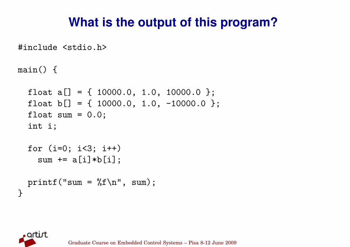
What is the output of this program?

#include <stdio.h>

main() {

float a[] = { 10000.0, 1.0, 10000.0 };

float b[] = { 10000.0, 1.0, -10000.0 };

float sum = 0.0;

int i;

for (i=0; i<3; i++)

sum += a[i]*b[i];

printf("sum = %f\n", sum);

}


Remarks:

• The result depends on the order of the operations

• Finite-wordlength operations are neither associative nor

distributive


Arithmetic in Embedded Systems

Small microprocessors used in embedded systems typically do not

have hardware support for floating-point arithmetic

Options:

• Software emulation of floating-point arithmetic

– compiler/library supported

– large code size, slow

• Fixed-point arithmetic

– often manual implementation

– fast and compact


Fixed-Point Arithmetic

Represent all numbers (parameters, variables) using integers

Use binary scaling to make all numbers fit into one of the integer

data types, e.g.

• 8 bits (char, int8_t): [−128, 127]

• 16 bits (short, int16_t): [−32768, 32767]

• 32 bits (long, int32_t): [−2147483648, 2147483647]


Challenges

• Must select data types to get sufficient numerical precision

• Must know (or estimate) the minimum and maximum value of

every variable in order to select appropriate scaling factors

• Must keep track of the scaling factors in all arithmetic

operations

• Must handle potential arithmetic overflows


Fixed-Point Representation

In fixed-point representation, a real number x is represented by an

integer X with N = m+ n+ 1 bits, where

• N is the wordlength

• m is the number of integer bits (excluding the sign bit)

• n is the number of fractional bits

Sign bit Integer bits Fractional bits

0 00 11111

“Q-format”: X is sometimes called a Qm.n or Qn number


Conversion to and from fixed point

Conversion from real to fixed-point number:

X := round(x ⋅ 2n)

Conversion from fixed-point to real number:

x := X ⋅ 2−n

Example: Represent x = 13.4 using Q4.3 format

X = round(13.4 ⋅ 23) = 107 (= 011010112)


A Note on Negative Numbers

In almost all CPUs today, negative integers are handled using

two’s complement: A “1” in the sign bit means that 2N should be

subtracted

Example (N = 8):

Binary representation Interpretation

00000000 0

00000001 1...

...

01111111 127

10000000 -128

10000001 -127...

...

1111111 -1


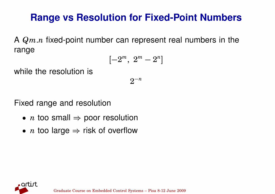
Range vs Resolution for Fixed-Point Numbers

A Qm.n fixed-point number can represent real numbers in the

range

[−2m, 2m − 2n]

while the resolution is

2−n

Fixed range and resolution

• n too small [ poor resolution

• n too large [ risk of overflow


Fixed-Point Addition/Subtraction

Two fixed-point numbers in the same Qm.n format can be added

or subtracted directly

The result will have the same number of fractional bits

z = x + y \ Z = X + Y

z = x − y \ Z = X − Y

• The result will in general require N + 1 bits; risk of overflow


Example: Addition with Overflow

Two numbers in Q4.3 format are added:

x = 12.25 [ X = 98

y = 14.75 [ Y = 118

Z = X + Y = 216

This number is however out of range and will be interpreted as

216− 256 = −40 [ z = −5.0


0 0 00

0 0 0

0 0 000

1 1 11

1 1 111

111

+

=


Fixed-Point Multiplication and Division

If the operands and the result are in the same Q-format,

multiplication and division are done as

z = x ⋅ y \ Z = (X ⋅ Y)/2n

z = x/y \ Z = (X ⋅ 2n)/Y

• Double wordlength is needed for the intermediate result

• Division by 2n is implemented as a right-shift by n bits

• Multiplication by 2n is implemented as a left-shift by n bits

• The lowest bits in the result are truncated (round-off noise)

• Risk of overflow


Example: Multiplication

Two numbers in Q5.2 format are multiplied:

x = 6.25 [ X = 25

y = 4.75 [ Y = 19

Intermediate result:

X ⋅ Y = 475

Final result:

Z = 475/22 = 118 [ z = 29.5

(exact result is 29.6875)


00 0

0

0

0000 0 00 0

0 00 0

00 00 0

111 11

11 1

1

1 1 1 1

1 1

111$

=


Multiplication of Operands with Different Q-format

In general, multiplication of two fixed-point numbers Qm1.n1 and

Qm2.n2 gives an intermediate result in the format

Qm1+m2.n1+n2

which may then be right-shifted n1+n2−n3 steps and stored in the

format

Qm3.n3

Common case: n2 = n3 = 0 (one real operand, one integer

operand, and integer result). Then

Z = (X ⋅ Y)/2n1


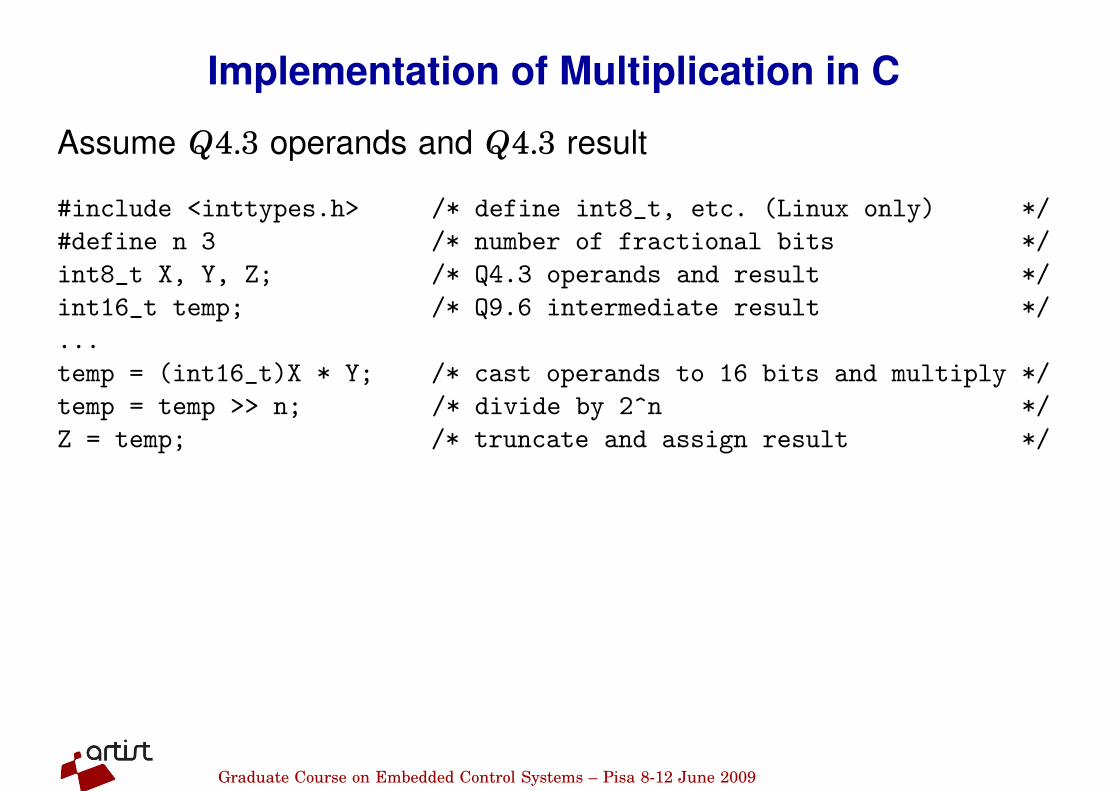
Implementation of Multiplication in C

Assume Q4.3 operands and Q4.3 result

#include <inttypes.h> /* define int8_t, etc. (Linux only) */

#define n 3 /* number of fractional bits */

int8_t X, Y, Z; /* Q4.3 operands and result */

int16_t temp; /* Q9.6 intermediate result */

...

temp = (int16_t)X * Y; /* cast operands to 16 bits and multiply */

temp = temp >> n; /* divide by 2^n */

Z = temp; /* truncate and assign result */


Implementation of Multiplication in C with Rounding

and Saturation

#include <inttypes.h> /* defines int8_t, etc. (Linux only) */




...

temp = (int16_t)X * Y; /* cast operands to 16 bits and multiply */

temp = temp + (1 << n-1); /* add 1/2 to give correct rounding */

temp = temp >> n; /* divide by 2^n */

if (temp > INT8_MAX) /* saturate the result before assignment */

Z = INT8_MAX;

else if (temp < INT8_MIN)

Z = INT8_MIN;

else

Z = temp;


Implementation of Division in C with Rounding

#include <inttypes.h> /* define int8_t, etc. (Linux only) */




...

temp = (int16_t)X << n; /* cast operand to 16 bits and shift */

temp = temp + (Y >> 1); /* Add Y/2 to give correct rounding */

temp = temp / Y; /* Perform the division (expensive!) */

Z = temp; /* Truncate and assign result */


Example: Atmel mega8/16 instruction set

Mnemonic Description # clock cycles

ADD Add two registers 1

SUB Subtract two registers 1

MULS Multiply signed 2

ASR Arithmetic shift right (1 step) 1

LSL Logical shift left (1 step) 1

• No division instruction; implemented in math library using

expensive division algorithm


Example Evaluation of Execution Time and Code

Size

• Atmel AVR ATmega16 microcontroller @14.7 MHz with

16K ROM controlling a rotating DC servo

ø 0.8� ø 0.8

ø 0‚95

øּ0,3

ø 0,8

ø 0,8

ø 0,8

ø 0,8

ø 0‚8

ø 0,8

øּ0,65

ø 0,8� ø 0,8

ø 0,95

øּ0,3

ø 0.8� ø 0.8

ø 0‚8

ø 0‚95

øּ0,3

øּ0,65

øּ0,65ø 0,5 ø 0,5�ø 0,5 øּ0,65

øּ0,65

ø 0‚8

1

s

k

Js +ּdΣωω

gnd

FRICTION

COMPENSATION

ON

POWER� SAT. OVL.�RESET POS.RESET

LTH ReglerteknikּR/B 88

θx0,1

x0,2

x0,1

x0,2

-1-1-1

Current

magnitude

4V/A

Ext. in

Moment

Ext. Int. +

LTH Reglerteknik RB 88

Int

OffOff

Reference

Ref out

• C program that implements simple state feedback controllers

– velocity control (one state is measured)

– position control (two states are measured)

• Comparison of floating-point and fixed-point implementations


Example Evaluation: Fixed-Point Implementation

The position controller (with integral action) is given by

u(k) = l1y1(k) + l2y2(k) + l3 I(k)

I(k+ 1) = I(k) + r(k) − y2(k)

where

l1 = −5.0693, l2 = −5.6855, l3 = 0.6054

Choose fixed-point representations assuming word length N = 16

• y1, y2, u, r are integers in the interval [−512, 511] ∈ Q10.0

• Let I ∈ Q16.0 to simplify the addition

• Use Q4.12 for the coefficients, giving

L1 = −20764, L2 = −23288, L3 = 2480


Example Evaluation: Pseudo-C Code

#define L1 -20764 /* Q4.12 */

#define L2 -23288 /* Q4.12 */

#define L3 2480 /* Q4.12 */

#define QF 12 /* number of fractional bits in L1,L2,L3 */

int16_t y1, y2, r, u, I=0; /* Q16.0 variables */

for (;;) {

y1 = readInput(1); /* read Q10.0, store as Q16.0 */

y2 = readInput(2); /* read Q10.0, store as Q16.0 */

r = readReference();

u = ((int32_t)L1*y1 + (int32_t)L2*y2 + (int32_t)L3*I) >> QF;

if (u >= 512) u = 511; /* saturate to fit into Q10.0 output */

if (u < -512) u = -512;

writeOutput(u); /* write Q10.0 */

I += r - y2; /* TODO: saturation and tracking... */

sleep();

}


Example Evaluation: Measurements

Floating-point implementation using float s:

• Velocity control: 950 µs

• Position control: 1220 µs

• Total code size: 13708 bytes

Fixed-point implementation using 16-bit integers:

• Velocity control: 130 µs

• Position control: 270 µs

• Total code size: 3748 bytes

One A-D conversion takes about 115 µs. This gives a 25–50

times speedup for fixed point math compared to floating point. The

floating point math library takes about 10K (out of 16K available!)


Controller Realizations

A linear controller

H(z) =b0 + b1z

−1 + . . .+ bnz−n

1+ a1z−1 + . . .+ anz−n

can be realized in a number of different ways with equivalent input-

output behavior, e.g.

• Direct form

• Companion (canonical) form

• Series (cascade) or parallel form


Direct Form

The input-output form can be directly implemented as

u(k) =

n∑

i=0

biy(k− i) −

n∑

i=1

aiu(k− i)

• Nonminimal (all old inputs and outputs are used as states)

• Very sensitive to roundoff in coefficients

• Avoid!


Companion Forms

E.g. controllable or observable canonical form

x(k+ 1) =

−a1 −a2 ⋅ ⋅ ⋅ −an−1 −an

1 0 0 0

0 1 0 0...

0 0 1 0

x(k) +

1

0...

0

y(k)

u(k) =

b1 b2 ⋅ ⋅ ⋅ bn

x(k)

• Same problem as for the Direct form

• Very sensitive to roundoff in coefficients

• Avoid!


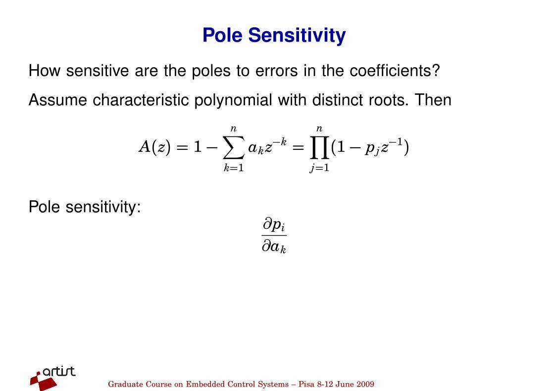
Pole Sensitivity

How sensitive are the poles to errors in the coefficients?

Assume characteristic polynomial with distinct roots. Then

A(z) = 1−

n∑

k=1

akz−k =

n∏

j=1

(1− pj z−1)

Pole sensitivity:�pi�ak


The chain rule gives

�A(z)

�pi

�pi�ak

=�A(z)

�ak

Evaluated in z = pi we get

�pi�ak

=pn−ki

∏n

j=1, j ,=i(pi − pj)

• Having poles close to each other is bad

• For stable filter, an is the most sensitive parameter


Better: Series and Parallel Forms

Divide the transfer function of the controller into a number of first-

or second-order subsystems:

+

Direct Form Series Form

Parallel Form

H(z)

H1(z)

H1(z)

H2(z)

H2(z)

• Try to balance the gain such that each subsystem has about

the same amplification


Example: Series and Parallel Forms

C(z) =z4 − 2.13z3 + 2.351z2 − 1.493z+ 0.5776

z4 − 3.2z3 + 3.997z2 − 2.301z+ 0.5184(Direct)

=( z2 − 1.635z+ 0.9025

z2 − 1.712z+ 0.81

)( z2 − 0.4944z+ 0.64

z2 − 1.488z+ 0.64

)

(Series)

= 1+−5.396z+ 6.302

z2 − 1.712z+ 0.81+6.466z− 4.907

z2 − 1.488z+ 0.64(Parallel)


Direct form with quantized coefficients (N = 8, n = 4):

Bode Diagram

Frequency (rad/sec)

Phase (

deg)

Magnitude (

dB

)

−20

0

20

40

C(z)C(z) direct form N=8

103

104

105

−225

−180

−135

−90

−45

0


Pole−Zero Map

Real Axis

Imag A

xis

−1 −0.5 0 0.5 1−1

−0.8

−0.6

−0.4

−0.2

0

0.2

0.4

0.6

0.8

1


Series form with quantized coefficients (N = 8, n = 4):

Bode Diagram

Frequency (rad/sec)

Phase (

deg)

Magnitude (

dB

)

−20

−10

0

10

20

30

C(z)C(z) series form N=8

103

104

105

−225

−180

−135

−90

−45

0


Pole−Zero Map

Real Axis

Ima

g A

xis C(z)

C(z) cascade form N=8

−1 −0.5 0 0.5 1−1

−0.5

0

0.5

1


Jackson’s Rules for Series Realizations

How to pair and order the poles and zeros?

Jackson’s rules (1970):

• Pair the pole closest to the unit circle with its closest zero.

Repeat until all poles and zeros are taken.

• Order the filters in increasing or decreasing order based on

the poles closeness to the unit circle.

This will push down high internal resonance peaks.


Well-Conditioned Parallel Realizations

Assume nr distinct real poles and nc distinct complex-pole pairs

Modal (a.k.a. diagonal/parallel/coupled) form:

zi(k+ 1) = λ izi(k) + β iy(k) i = 1, . . . ,nr

vi(k+ 1) =

σ i ω i

−ω i σ i

vi(k) +

γ i1

γ i2

y(k) i = 1, . . . ,nc

u(k) = Dy(k) +

nr∑

i=1

γ izi(k) +

nc∑

i=1

δ Ti vi(k)

Matlab: sysm = canon(sys,’modal’)


Possible Pole Locations for Direct vs Modal Form

0 0.2 0.4 0.6 0.8 10

0.1

0.2

0.3

0.4

0.5

0.6

0.7

0.8

0.9

1

Real

Imag

Pole positions with N=6 bits, direct form

0 0.2 0.4 0.6 0.8 10

0.1

0.2

0.3

0.4

0.5

0.6

0.7

0.8

0.9

1

Real

Imag

Pole positions with N=6 bits, modal form


Short Sampling Interval Modification

In the state update equation

x(k+ 1) = Φx(k) + Γy(k)

the system matrix Φ will be close to I if h is small. Round-off

errors in the coefficients of Φ can have drastic effects.

Better: use the modified equation

x(k+ 1) = x(k) + (Φ − I)x(k) + Γy(k)

• Both Φ − I and Γ are roughly proportional to h

– Less round-off noise in the calculations

• Also known as the δ -form


Short Sampling Interval and Integral Action

Fast sampling and slow integral action can give roundoff problems:

I(k+ 1) = I(k) + e(k) ⋅ h/Ti︸︷︷︸

(0

Possible solutions:

• Use a dedicated high-resolution variable (e.g. 32 bits) for the

I-part

• Update the I-part at a slower rate

General problem for filters with very different time constants


fix point implementation of clalihcontrol algorithms

Documents