five centuries of upper indus river flow from tree rings

Five centuries of Upper Indus River flow from tree rings

Edward R. Cook a,⇑, Jonathan G. Palmer b,c, Moinuddin Ahmed d, Connie A. Woodhouse e, Pavla Fenwick c,Muhammad Usama Zafar d, Muhammad Wahab d, Nasrullah Khan d

a Tree Ring Laboratory, Lamont-Doherty Earth Observatory, Columbia University, Route 9W, Palisades, NY 10964, USAb Climate Change Research Centre (CCRC), School of Biological, Earth and Environmental Sciences, The University of New South Wales, Sydney 2052, NSW, Australiac Gondwana Tree-ring Laboratory, P.O. Box 14, Little River, Canterbury 7546, New Zealandd Botany Department, Federal Urdu University of Arts Science and Technology, Gulshan-e Iqbal, Karachi, Sind 75300, Pakistane School Geography and Development, University of Arizona, P.O. Box 210076, Tucson, AZ 85721, USA

a r t i c l e i n f o

Article history:Received 29 October 2012Received in revised form 1 February 2013Accepted 2 February 2013Available online xxxxThis manuscript was handled byKonstantine P. Georgakakos, Editor-in-Chief

Keywords:DendroclimatologyUpper Indus Basin dischargeStreamflow reconstruction from tree ringsSemi-parametric prediction intervalsDischarge regime shifts

s u m m a r y

Water wars are a prospect in coming years as nations struggle with the effects of climate change, growingwater demand, and declining resources. The Indus River supplies water to the world’s largest contiguousirrigation system generating 90% of the food production in Pakistan as well as 13 gigawatts of hydroelectric-ity. Because any gap between water supply and demand has major and far-reaching ramifications, anunderstanding of natural flow variability is vital – especially when only 47 years of instrumental recordis available. A network of tree-ring sites from the Upper Indus Basin (UIB) was used to reconstruct river dis-charge levels covering the period AD 1452–2008. Novel methods tree-ring detrending based on the ‘signalfree’ method and estimation of reconstruction uncertainty based on the ‘maximum entropy bootstrap’ areused. This 557-year record displays strong inter-decadal fluctuations that could not have been deducedfrom the short gauged record. Recent discharge levels are high but not statistically unprecedented andare likely to be associated with increased meltwater from unusually heavy prior winter snowfall. A periodof prolonged below-average discharge is indicated during AD 1572–1683. This unprecedented low-flowperiod may have been a time of persistently below-average winter snowfall and provides a warning forfuture water resource planning. Our reconstruction thus helps fill the hydrological information vacuumfor modeling the Hindu Kush–Karakoram–Himalayan region and is useful for planning future developmentof UIB water resources in an effort to close Pakistan’s ‘‘water gap’’. Finally, the river discharge reconstructionprovides the basis for comparing past, present, and future hydrologic changes, which will be crucial fordetection and attribution of hydroclimate change in the Upper Indus Basin.

! 2013 Elsevier B.V. All rights reserved.

1. Introduction

Pakistan is located in an extremely arid region, with an averagerainfall of less than 240 mm a year making it ‘‘one of the world’smost water-stressed countries’’ (World Bank, 2005). The rapidlygrowing population and economy are heavily dependent on waterfrom the Indus River Basin to supply the largest contiguous irriga-tion system in the world that in turn yields 90% of the food produc-tion in Pakistan (Qureshi, 2011). The overall basin consists of sixmain rivers (the Indus, Jhelum, Chenab, Ravi, Sutlej, and Kabul)originating from glaciers in the Karakoram and western Himalaya.Collectively these rivers provide irrigation water to more than16 million hectares of agricultural land and generate up to 13 giga-watts of electricity through hydropower plants in Pakistan, India,and Afghanistan (ICIMOD, 2010). Thus, as the Indus River Basingoes, so goes Pakistan.

The Indus River itself contributes about 43% of the total annualflow of the basin, and 72% of that discharge comes from the‘‘Northern Areas’’ of Pakistan (Ahmed and Joyia, 2003). The latterconstitutes the Upper Indus Basin (UIB), which provides waterfor the storage lake behind Tarbela Dam as the river emerges fromthe mountains. This reservoir was primarily designed for irrigationand provides canal irrigation water for a substantial fraction ofPakistan’s agricultural production. It also has an installed hydro-electric capacity of 3478 MW, which amounts to 49% of Pakistan’stotal hydroelectric power capacity (http://environmentdefenc-er.wordpress.com/tag/tarbela-dam/). So without question, ade-quate UIB discharge into Tarbela Reservoir is crucial to theeconomic and social wellbeing of the people of Pakistan.

The potential vulnerability of Pakistan to changes in UIBstreamflow is indicated by recent events [or conditions]. In March2012, the water level of Tarbela Reservoir dropped to ‘‘dead level’’(http://tribune.com.pk/story/346909/water-in-tarbela-dam-touches-dead-level/), the point at which useful water yield is zero, andas of August 2012, the water level was still below normal due to

0022-1694/$ - see front matter ! 2013 Elsevier B.V. All rights reserved.http://dx.doi.org/10.1016/j.jhydrol.2013.02.004

⇑ Corresponding author. Tel.: +1 845 365 8618.E-mail address: [email protected] (E.R. Cook).

Journal of Hydrology xxx (2013) xxx–xxx

Contents lists available at SciVerse ScienceDirect

Journal of Hydrology

journal homepage: www.elsevier .com/ locate / jhydrol

Please cite this article in press as: Cook, E.R., et al. Five centuries of Upper Indus River flow from tree rings. J. Hydrol. (2013), http://dx.doi.org/10.1016/j.jhydrol.2013.02.004

http://environmentdefencer.wordpress.com/tag/tarbela-dam/

http://environmentdefencer.wordpress.com/tag/tarbela-dam/

http://tribune.com.pk/story/346909/water-in-tarbela-dam-touches-dead-level/

http://tribune.com.pk/story/346909/water-in-tarbela-dam-touches-dead-level/

http://dx.doi.org/10.1016/j.jhydrol.2013.02.004

mailto:[email protected]


http://www.sciencedirect.com/science/journal/00221694

http://www.elsevier.com/locate/jhydrol



insufficient inflow of snow and glacier meltwater into the reservoirbecause of below-average prior winter snows in the mountains(http://www.geo.tv/GeoDetail.aspx?ID=63047). ‘‘Dead level’’ mayoccur from time to time due to the normal seasonal drawdownof water based on irrigation and hydropower demands, but thefailure of the UIB to refill the reservoir to normal levels so late inthe principal runoff season is alarming. This is an example of the‘‘water gap’’ between supply and demand that is increasingly fac-ing Pakistan now (World Bank, 2005).

Thus, an obvious question is how reliable is the UIB for provid-ing enough discharge to support both irrigation and hydropowergeneration needs? This is an open question because so little isknown about the long-term properties of the UIB hydrologic re-gime and its principal contributors, snow and glacier meltwater.The most representative record of total discharge into Tarbela Res-ervoir is upstream at Besham and it only begins in 1969 (Archer,2003), a short 44-year long record that is inadequate for modelingthe long-term properties of river discharge (Rodriguez-Iturbe,1969). In addition, the short streamflow records available provideno context for assessing recent trends and shifts in flow volume.These problems echo the more general concern voiced by Pel-licciotti et al. (2012) over the ‘‘striking scarcity of hydro-meteoro-logical and glaciological data’’ for hydrological modeling of theHindu Kush–Karakoram–Himalayan region.

We address part of this information need through the recon-struction of UIB runoff from long, climatically sensitive, annualtree-ring chronologies in northern Pakistan. Specifically, we pres-ent a calibrated and validated reconstruction of runoff for the peakMay–September discharge season for the UIB. This reconstructionextends back to 1452 C.E. As such, it provides a far more completerecord of discharge variability and change over a range of time-scales from annual to centennial and over a range of climate statesfrom the early stages of the ‘‘Little Ice Age’’ (Gove, 1988) to the cur-rent epoch of anthropogenic climate change in the 20th and 21stcenturies, referred to by some as the ‘‘Anthropocene’’ (Crutzen,2002). River flow reconstructions of the kind presented here (cf.,Stockton and Jacoby, 1976; Cook and Jacoby, 1983; Cleaveland,1999; Woodhouse et al., 2006; Meko et al., 2007) have greatly in-creased our understanding of how discharge has varied over timein ways not possible from the relatively short gauged records thatare typically available.

2. Upper Indus Basin discharge at Partab Bridge

The UIB discharge record at Partab Bridge (34"430N, 74"380E;elev. 1250 m; Fig. 1; Archer, 2003) was chosen for tree-ring recon-struction because it is the longest, most representative, dischargerecord for the UIB. It represents 145,618 km2 or 87.7% of the

Fig. 1. Map of the Upper Indus Basin in Pakistan showing the Indus River and its main tributaries in blue and the locations of the tree-ring chronologies (open red triangles)used for reconstructing May–September discharge at Partab Bridge (inverted filled black triangle). The tree species used for reconstruction are Abies pindrow, Juniperus excelsa,Cedrus deodara, Picea smithiana, Pinus gerardiana, and Pinus wallichiana. The three sizes of open tree-ring triangles are scaled by correlation with discharge (small: 0.30–0.39,medium: 0.40–0.49, large: P0.50). The more highly correlated tree rings tend to be closer to the Partab Bridge record. The filled black dots are the cities of Peshawar andIslamabad. The map is courtesy of Paul J. Krusic and Generic Mapping Tools. (For interpretation of the references to colour in this figure legend, the reader is referred to theweb version of this article.)

2 E.R. Cook et al. / Journal of Hydrology xxx (2013) xxx–xxx


http://www.geo.tv/GeoDetail.aspx?ID=63047



gauged basin area draining into Tarbela Reservoir at Besham (Al-ford, 2011; Sharif et al., 2012) and begins in 1962, making itslightly longer than the Besham record. Monthly data for thisgauge was previously made available for study by the PakistanWater and Power Development Authority (WAPDA) for the years1962–1996 (e.g., Archer, 2003). Subsequently, WAPDA providedus with streamflow updates to 2008 for the Indus and its majortributaries upstream from Partab Bridge, but not for Partab Bridgeitself. Fortunately, these post-1996 upstream updates allowed usto usefully extend the Partab Bridge record to 2008 with a high de-gree of accuracy.

The specific monthly discharge records used for estimating Par-tab Bridge from 1997 to 2008 were:

(a) Indus River at Kachora (35"270N, 75"250E) for 1970–2008.(b) Hunza River at Dainyor (35"560N, 74"230E) for 1966–2008

(missing: 2005, 2006, and 2007).(c) Gilgit River at Gilgit (35"560N, 74"180E) for 1960–2008 (miss-

ing: July–December, 1999).

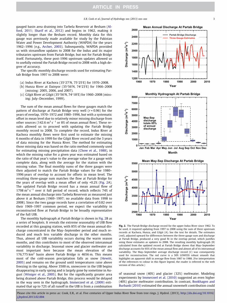
The sum of the mean annual flows for these gauges match thepattern of discharge at Partab Bridge very well (r = 0.96) for theyears of overlap, 1970–1972 and 1980–1996, but with a systematicoffset in mean level due to relatively minor missing discharge fromother sources (142.6 m3 s!1 or 8% of mean annual flow). These re-sults allowed us to proceed with updating the Partab Bridgemonthly record to 2008. To complete the record, Indus River atKachora monthly flows were first used to estimate the missing6 months of data in 1999 for the Gilgit River record and the 3 yearsof data missing for the Hunza River. The method for estimatingthose missing data was based on the ratio method commonly usedfor estimating missing precipitation data (Chow et al., 1988), inwhich the missing value for a given year was estimated based onthe ratio of that year’s value to the average value for a gauge withcomplete data, along with the average for the station with themissing value. The final monthly sums of the three gauges werethen adjusted to match the Partab Bridge values for the 1980–1996 years of overlap to account for offsets in mean level. Theresulting three-gauge sum matches the flow at Partab Bridge forthe years of overlap with a mean offset of only +0.2% (Fig. 2A).The updated Partab Bridge record has a mean annual flow of1798 m3 s!1 over it full period of record, which reflects 74% ofthe mean annual discharge into Tarbela Reservoir as measured justabove it at Besham (1969–1997; no available data from 1998 to2008). Since the two gauge records have a correlation of 0.82 overtheir 1969–1997 common period, we expect the variability inreconstructed flow at Partab Bridge to be broadly representativeof the full UIB.

The monthly hydrograph at Partab Bridge is shown in Fig. 2B asa series of boxplots. It reveals the extreme seasonality of UIB flowrecorded at this gauging station, with 85% of the mean annual dis-charge concentrated in the May–September period and much re-duced and much less variable discharge in the other months.Thus, almost all UIB variability occurs during the warm seasonmonths, and this contributes to most of the observed interannualvariability in discharge. Seasonal snow and glacier meltwater aremost important here because the mean elevation of the176,775 km2 basin above Partab Bridge is 4656 m. This meansmost of the cold-season precipitation falls as snow (Hewitt,2005) and remains on the ground until temperatures raise abovefreezing in the spring. Above 3500 m, snowcover in the UIB beginsdisappearing in early spring and is largely gone by sometime in Au-gust (Winiger et al., 2005). But for the significantly greater areabeing drained above Partab Bridge, this process would be delayedin the way seen in the hydrograph. Immerzeel et al. (2009) esti-mated that up to 72% of all runoff in the UIB is from a combination

of seasonal snow (40%) and glacier (32%) meltwater. Modelingexperiments by Immerzeel et al. (2010) suggested an even higher(40%) glacier meltwater contribution. In contrast, Bookhagen andBurbank (2010) estimated the annual snowmelt contribution could

0

1000

2000

3000

4000

5000

6000

7000

8000

Jan Feb Mar Apr May Jun Jul Aug Sep Oct Nov Dec

Monthly Hydrograph At Partab Bridge

Month

May-Sepdischargetotals 85%of annualdischarge

2500

3000

3500

4000

4500

5000

5500

1960 1970 1980 1990 2000 2010

Mean May-Sep Discharge At Partab Bridge

Year

Disc

harg

e (m

3 s-1

)Di

scha

rge

(m3 s

-1)

Disc

harg

e (m

3 s-1

)

1200

1400

1600

1800

2000

2200

2400

2600

1960 1970 1980 1990 2000 2010

Mean Annual Discharge At Partab Bridge

Partab Bridge Discharge Three-Gauge Estimates

Year

Fig. 2. The Partab Bridge discharge record for the upper Indus River since 1962. Tobe used, it required updating from 1997 to 2008 using the sum of three upstreamrecords at Kachora, Hunza, and Gilgit (A). See the text for details. The estimates(red), adjusted upward for differences between the three-gauge sum and dischargeat Partab Bridge, produced a very good fit in the overlap period, which justifiesusing those estimates as updates to 2008. The resulting monthly hydrograph (B)calculated from the updated record at Partab Bridge shows that May–Septemberdischarge accounts for 85% of the mean annual flow and almost all of its interannualvariability. The May–September average discharge record (C) was consequentlyused for reconstruction. The red curve is a 50% LOWESS robust smooth thathighlights an apparent shift in average flow from 1987 to 1988. (For interpretationof the references to colour in this figure legend, the reader is referred to the webversion of this article.)

E.R. Cook et al. / Journal of Hydrology xxx (2013) xxx–xxx 3




be as high as 66% in the UIB, which is more in line with an evenhigher estimate of 82% between late-spring snowcover area andsubsequent streamflow recorded at Besham from 1969 to 1973(Rango et al., 1977). There is clearly much uncertainty concerningthe relative contributions of snow and glacier meltwater to UIBdischarge.

Based on the monthly hydrograph, May–September dischargeat Partab Bridge was chosen as the season to reconstruct becauseit encompasses most of the annual discharge and almost all of itsinterannual variability. Of equal importance, May–Septemberbroadly matches the extended physiologically active season ofthe trees used here for reconstruction. This discharge record isshown in Fig. 2C. It has a correlation of 0.996 with the mean annualseries (Fig. 2A), with the same regime-like shift in discharge from1987 to 1988. The step-like increase in river flow since 1988 couldbe related to increased seasonal snowfall in the upper elevations,which has a maximum accumulation between 5000 and 6000 m(Hewitt, 2005), or perhaps increased glacier meltwater. At lowerelevations, Archer and Fowler (2004) reported an increase in win-ter precipitation from 1961 to 1999 at several locations in theKarakoram range. A simple trend line fit to the discharge data from1962 to 1999 also yields a positive trend (r = 0.33; p < 0.05), whichis consistent with the results of Archer and Fowler (2004). How-ever, this trend is neither gradual nor homogeneous. Rather, it islargely driven by the abrupt jump in discharge beginning in1988. Immerzeel et al. (2009) later used MODIS satellite measure-ments to construct a seasonal snow cover record from 2000 to2008 for the UIB, which post-dates the abrupt increase in dis-charge. In contrast to the previous results, they found evidencefor a decreasing trend in winter snow cover in two elevation zonesabove 4700 m, with the highest zone above 5000 m having thestrongest negative trend. The robust LOWESS smooth (Fig. 2C) alsoshows evidence for a weak negative trend in May–September dis-charge since 2000. Consistent with this suggestion, Shekhar et al.(2010) likewise reported a weak negative trend in KarakoramNovember–April snowfall since 1991/92. A similar weak trend isevident in the discharge data from 1992 to 2008. Unfortunately,none of these studies of winter precipitation change provide anyinsights into the cause of the jump in streamflow from 1987 to1988.

An abrupt increase in glacier meltwater has not been consid-ered thus far as a contributor to the jump in May–September dis-charge increase since 1988. The consensus opinion is that theglaciers of the Karakoram are reasonably stable (Hewitt, 2005;Schmidt and Nusser, 2009; Armstrong, 2010; Bolch et al., 2012;Gardelle et al., 2012), which implies that the glacier meltwatercontribution over the 1962–2008 period has probably not in-creased enough to explain the increase in discharge. In addition,the Karakoram range has experienced a decreasing trend inspring/summer temperatures since the 1960s (Fowler and Archer,2006; Shekhar et al., 2010), which argues for an actual decrease inglacier meltwater flux since 1988. In contrast, Immerzeel et al.(2009) argued that the Karakoram have in fact warmed over thepast few decades. Paradoxically, their analyses are based on grid-ded temperature data based on some of the same station data usedby Fowler and Archer (2006). Why these apparent differences existis not clear.

Viewed in its entirety, observed May–September discharge atPartab Bridge can be interpreted in different ways. One plausibleinterpretation (akin to a null hypothesis here) is that warm-seasonUIB discharge has been experiencing natural interdecadal variabil-ity since 1962 around a relatively stationary long-term mean of3674 ± 77 m3 s!1 (±1 standard error). The data also allow for twoquite different alternate hypotheses: (1) that near-normal flow oc-curred from 1962 to 1987 (3470 ± 95 m3 s!1) followed by anoma-lously high flow from 1988 to 2008 (3926 ± 105 m3 s!1), or (2)

that anomalously low-flow occurred from 1962 to 1987 followedby a return to essentially normal flow from 1988 to 2008. Eitherway, a t-test of the difference between the two means (assumingnormality, independence, and unequal variances) is statisticallysignificant (p < 0.002), but the two alternate hypotheses are quitedifferent in their hydrological interpretations. With only 47 yearsof UIB discharge data roughly split in half by the two putative re-gimes, it is impossible to say if either of these alternate hypothesesis more plausible than the null hypothesis based on all the data.The uncertainties in the statistical properties of such short hydro-logic records are too large to provide useful estimates of long-termflow characteristics for modeling and simulation (Rodriguez-Iturbe, 1969). These limitations indicate why a multi-centennialtree-ring reconstruction of UIB discharge would be so useful be-cause it would put into long-term context the pattern of variabilityobserved in the short Partab Bridge discharge record and provideimproved estimates of its statistical properties at interdecadaland longer time scales (cf. Woodhouse et al., 2006; Meko et al.,2007).

3. The Upper Indus Basin tree-ring network

The high-elevation conifer forests of the UIB contain a diversemix of tree species that can be used for reconstructions of past cli-mate. This potential was first demonstrated by Ahmed (1989) forthe Himalayan fir Abies pindrow and further documented by Esperet al. (1995) through the detailed sampling and analysis of the juni-per species Juniperus excelsa in and around the Hunza Valley regionof northern Pakistan. Other tree species available for sampling in-clude Cedrus deodara, Pinus gerardiana, Pinus wallichiana and Piceasmithiana (Ahmed and Sarangezai, 1991; Ahmed and Naqvi,2005; Ahmed et al., 2011). Given this potential, and support fromthe Pakistan-U.S. Science and Technology Cooperation Program, aconcerted effort was made to develop a dense multi-species tree-ring network for reconstructing UIB discharge. This effort resultedin a network of 39 well-replicated annual tree-ring chronologies(see Ahmed et al., 2011), all precisely dated following standarddendrochronological cross-dating techniques (Stokes and Smiley,1968). Of the 39 chronologies, 26 are new, including two locatedin far eastern Afghanistan, while the remaining 13 (all J. excelsa)are from earlier collections by Esper et al. (1995). Several speciesin this network have trees with ages up to "700 years (C. deodara,P. gerardiana, P. wallichiana and P. smithiana), but J. excelsa is thelongest lived with some trees exceeding 1000 years of age.

The raw ringwidth measurement data for each of the 39 sitesare annual records of radial tree growth measured in units of mil-limeters per year. As such they contain non-climatic growth trendsrelated to biological and geometrical constraints on radial growth.These non-climatic trends are typically removed through curve fit-ting and detrending by a procedure called ‘tree-ring standardiza-tion’ (Fritts, 1976; Cook and Kairiukstis, 1990). Here, we usedetrending based on the relatively new ‘signal free’ (SF) method(Melvin and Briffa, 2008), which is designed to enhance the preser-vation of common medium-frequency variance (timescales of dec-ades to a century or more) in tree chronologies. Using the SFmethod, ‘‘trend distortion’’ effects during the detrending phase oftree-ring chronology development are eliminated. This problemis caused by the influence of common persistent medium-fre-quency signals (e.g. increases in growth caused by climate) onthe fitting of the detrending curves. This common signal can biasthe removal of supposed ‘‘non-climate’’ variance, leading to distor-tion of the external forcing signal in tree-ring chronologies (Melvinand Briffa, 2008). Trend distortion is most prevalent at the ends ofthe chronologies, but can occur anywhere in a tree-ring serieswhen flexible curve fitting methods (e.g. smoothing splines; Cook





and Peters, 1981) are used. As such, the SF method can also correctfor lost common medium-frequency variance and mitigate the ef-fects of the ‘segment length curse’ (Cook et al., 1995) on the pres-ervation of variability in excess of the lengths of the tree-ring seriesused in chronology development. We have performed SF standard-ization on all of our tree-ring chronologies used for reconstructionof May–September discharge at Partab Bridge. In so doing, it is pos-sible to evaluate the properties of UIB streamflow from interannualto centennial timescales.

Intense environmental gradients are present in the Karakoram,as indicated by Archer and Blenkinsop (2010), who found high het-erogeneity between climate station data there. Correlations be-tween the 28 site chronologies (ranging from 2450 to3900 m.a.s.l.) were similarly investigated as a function of increas-ing separation distance between sites and species (Ahmed et al.,2011). A similar decline in correlation with increasing distancewas consistently found both between sites of the same speciesand between sites composed of different species. In some cases, amuch stronger correlation occurred between different speciesgrowing at the same site than between different sites of the samespecies, but separated by as little as 0.5 km. Such results highlightthe strong elevational gradients and highly variable slope aspectspresent in the Karakoram. Even so, Ahmed et al. (2011) showedthrough correlations between a subset of Karakoram tree ringschronologies used here and gridded monthly temperature and pre-cipitation data over the Karakoram region that there was a strongcommon climate signal among the chronologies. In most cases, thechronologies correlated positively with some or all of the January-to-May months of precipitation preceding the growing season andnegatively with some or all of the April-to-July months of temper-ature during the growing season. So it appears that seasonal snow-fall is the primary source of soil moisture for subsequent treegrowth in the Karakoram, with summertime temperature affectingradial growth through evapotranspiration demand during the pho-tosynthetically active warm season.

Archer and Blenkinsop (2010) argued that a reconstruction ofhydroclimate from tree rings in the Karakoram was unlikely tobe successful because of intense environmental gradients there.As we will show, this interpretation is unduly pessimistic. Thecombination of a sufficiently dense and diverse multi-speciestree-ring network and a well-tested statistical method for dendro-climatic reconstruction have successfully produced a skillful recon-struction of May–September discharge for the Upper Indus River atPartab Bridge covering the period 1452–2008.

4. The streamflow reconstruction method

For reconstruction of UIB discharge at Partab Bridge, we used aprincipal components regression (PCR) approach that has beenused previously to reconstruct climate from tree rings (Cooket al., 1999; 2004; Cook et al., 2010a, 2010b). This approach pro-duces a ‘nested’ suite of reconstructions (cf. Meko, 1997; Cooket al., 2002; Wilson et al., 2007) in which shorter tree-ring seriesused as predictors are sequentially eliminated from the predictorpool used in PCR until the pool is exhausted. Each of the nestedreconstructions is separated by at least 10 years. The full ‘nested’reconstruction is then created by appending each subset-recon-struction extension back in time to the beginning of pre-existingshorter reconstruction after appropriate scaling to recover lost var-iance due to regression in each reconstruction, thus producing thelongest possible reconstruction from the available tree-ring data.The scaling is done to insure that no artificial variability due to dif-ferences in regression R2 from nest to nest is present in the fullnested reconstruction. The recovery of lost variance due to regres-sion also provides for less biased comparisons of current with past

climate fluctuations, but at the cost of increased uncertainty in theestimates (Ammann et al., 2010). Since changes in mean dischargeare of primary interest here, this tradeoff is considered acceptable.

In developing tree-ring based reconstructions, it is important toassess model skill over the calibration period and over years thathave been withheld from the calibration for model validation. Foreach nested subset model, a suite of calibration and validation sta-tistics is produced., (e.g., Michaelsen, 1987; Meko, 1997; Cooket al., 1999, 2004, 2010a, 2010b): CRSQ (calibration period coeffi-cient of multiple determination or R2), CVRE (calibration periodreduction of error calculated by leave-one-out cross-validation),VRSQ (validation period square of the Pearson correlation or r2),VRE (validation period reduction of error) and VCE (validation per-iod coefficient of efficiency). VRE and VCE differ from VRSQ in theway that they use the calibration and validation period means,respectively, as baselines for assessing model skill. When positive,these statistics can all be interpreted as somewhat differentexpressions of variance in common between the actual and esti-mated data. However, unlike CRSQ, which can never be negative,CVRE, VRSQ (by retaining the negative sign of r after squaring),VRE and VCE can also be negative, indicating that there is no skillin the estimates. See Cook et al. (1999, 2004) for details. The diffi-culty in estimating the actual statistical significance of CVRE, VRE,and VCE even when positive has always been a problem because notheory-based tests of these statistics exist. This limitation has beenlargely eliminated here through the novel use of the maximum en-tropy bootstrap (MEBoot; Vinod, 2006; Vinod and López-de-Lacal-le, 2009) to estimate reconstruction uncertainties. In so doing, non-parametric uncertainties for all of the nested calibration and vali-dation statistics naturally emerge from the reconstructionprocedure.

Besides reporting the calibration/validation statistics describedabove, uncertainties on the estimates themselves are also providedin the form of regression prediction intervals (Seber and Lee, 2003;Olive, 2007) estimated as:

Y f # tn!p;1!a=2

ffiffiffiffiffiffiffiffiffiffiMSEp ffiffiffiffiffiffiffiffiffiffiffiffiffiffiffiffiffi

ð1þ hf Þq

ð1Þ

where Yf is the regression estimate, t is the 1!a/2 t-statistic with n–p degrees of freedom, MSE is the mean square error of the fitted cal-ibration model, and hf is the ‘‘leverage’’ from the hat-matrix of pre-dictors for each year calculated as:

hf ¼ xTf ðX

T XÞ!1xf ð2Þ

where X is the design matrix of predictors used for calibration and xf

is the vector of values used for prediction in year f. The primary dif-ference from Eq. (1) implemented here is that the fixed t-statistic(assume 90% 2-tailed limits) for scaling the uncertainties are re-placed by the variable 5th and 95th quantiles (90% quantile limits)from a suite of pseudo-reconstructions produced after applying ME-Boot to both the predictor and predictand data prior to regression.This includes any pre-processing of the original candidate tree-ringchronologies up to the final regression model (e.g., prewhiteningand predictor variable screening; cf. Cook et al., 1999). So, exceptfor the selection of the original pool of candidate tree-ring predic-tors and the preprocessing that is used to create those annualtree-ring chronologies, all steps in the regression modeling proce-dure are incorporated in the MEBoot procedure used here. Becausethe fixed t-statistic has now been replaced by the variable non-parametric MEBoot 90% quantiles, but the overall regression-basedparametric form of Eq. (1) remains intact, we refer to our uncertain-ties as semi-parametric prediction intervals. See Olive (2007) foralternative ways of modifying the calculation of prediction intervalsto make them more general.

The maximum entropy bootstrap is distinctly different from theclassical bootstrap (Efron, 1979) because it does not randomly





sample with replacement all of the available data, or in our case,data across time. To do so would break up the temporal order ofthe sequence, which is a defining property of the series. In contrast,MEBoot preserves the overall shape (i.e., the temporal order) of thedata, which allows for direct estimates of uncertainty to be madefrom the ensemble of MEBoot pseudo-reconstructions. MEBoot isalso unique in the way it preserves the persistence structure andoverall properties of any arbitrary stochastic process, includingthose that are non-stationary and heteroscedastic. This can be dif-ficult if not impossible to do using the moving block bootstrap (cf.Wilks, 1997). In so doing, MEBoot satisfies both the ergodic theo-rem and central limit theorem (Vinod and López-de-Lacalle,2009), which provides it with very nice asymptotic properties. Col-lectively, this guarantees that the overall stochastic properties ofthe original time series used in regression are well preserved inthe ensemble of MEBoot pseudo-series. Thus, MEBoot adds a natu-ral element of randomness to each pseudo-reconstruction, whilepreserving the overall stochastic properties of the predictor–pre-dictand data. In this sense MEBoot can be thought of as a perturba-tion method. See Vinod and López-de-Lacalle (2009) for details andVinod (2010) for a discussion on the use of MEBoot as a solution tothe spurious time series regression problem.

We applied MEBoot to both the tree-ring predictors and steam-flow predictand data here. This explicitly admits that there is someerror on both sides of the regression model equation to consider,but these errors are either unknown or very difficult to estimatewith much certainty. This makes the use of more formal ‘total leastsquares’ methods (e.g., Hegerl et al., 2007) difficult to apply be-cause the ratio of error variances of the predictors and predictandis assumed known or at least estimated in a reasonably precise andunbiased way. In lieu of explicitly estimating these weakly con-strained error variances, we use MEBoot as a perturbation methodthat imparts a reasonable level of random error to each series da-tum prior to regression modeling. This was done 300 times here (anumber sufficient for "90% intervals) to produce an empiricalprobability density function of uncertainty for each year as areplacement for the t-distribution. This non-parametric part ofthe prediction interval equation allows the estimated uncertaintiesto have variable coverage from year to year and to also be asym-metric as dictated by the data. Coupling these 90% quantile uncer-tainties with the MEBoot 95th quantile of MSE and hf (the upper90% quantile limit) for each reconstruction nest completes the esti-mation of the 90% semi-parametric prediction intervals.

The original parametric form of the prediction intervals in Eq.(1) has been preserved here, but it now estimates those intervalsin a more non-parametric, data-adaptive way. The leverage termscan also used to identify those years that fall outside the range ofthe calibration period data and thus behave as extrapolations(Weisberg, 2005). In these cases, the prediction intervals are farless reliable (Olive, 2007). Also, because 300 pseudo-reconstruc-tions have been estimated now for generating the semi-parametricprediction intervals, it follows that there are also 300 pseudo-esti-mates of the calibration and validation statistics described earlierfor generating their 90% uncertainty intervals, including those forVRE and VCE for which there are no theory-based confidence inter-vals available to calculate.

5. Tree-ring reconstruction of upper Indus River discharge

The nested reconstruction of UIB May–September dischargewas produced using the PCR approach described above. It is basedon a 24 tree-ring chronology subset of the 39 available from theUIB, using only those ending on or after 2005 in order to maintaina common time interval with the Partab Bridge discharge record,The 24 tree-ring chronologies begin anywhere from 1260 to 1738

and all end on or after 2005. However, the minimum acceptablesample size for each annual mean tree-ring index value in eachchronology was set to five to eliminate the more weakly replicatedand least reliable inner portions of the chronologies. This resultedin a change from 1260 to 1452 for the earliest start year and from1738 to 1800 for the latest start year.

The calibration period chosen to develop the nested regressionmodels was 1975–2004 (30 years), with the 1962–1974 perioddata (13 years) withheld for independent validation of the tree-ring estimates (cf. Fritts, 1976; Snee, 1977; Picard and Berk,1990). The validation period is relatively short, but this limitationis compensated for in the following section by comparisons ofthe reconstruction to fully independent tree-ring-based hydrocli-matic records from the UIB. Each chronology was evaluated for cor-relation with May–September discharge for both year t and t + 1 (atotal of 48 candidate predictors) and only those chronologies thatcorrelated significantly (p < 0.10, 2-tailed) were retained as predic-tors in PCR (cf. Cook et al., 1999). This screening procedure reducedthe predictor set from 48 candidates to 15 actually used in PCR.This included the retention of five tree species (A. pindrow, J. excel-sa, C. deodara, P. smithiana, P. gerardiana, and P. wallichiana), withall but two being positively correlated with discharge in year t.The climate correlation results of Ahmed et al. (2011) suggest thatthese positive correlations are related to a positive response towinter–spring precipitation and the subsequent contribution ofseasonal snowmelt to discharge. The geographic distribution ofchronologies used, size-coded by strength of correlation with dis-charge, is shown in Fig. 1. It can be seen that the distribution ofsites covers a large geographic portion of the Upper Indus River Ba-sin. The more highly correlated tree rings tend to be closer to thePartab Bridge gauging station.

The 15 screened tree-ring chronologies produced 12 nested dis-charge reconstructions, each created by sequentially running PCRon decreasing subsets of chronologies with progressively earlierstarting years. The complete nested reconstruction (Fig. 3) extendsfrom 1452 to 2004 (2005–08 are appended instrumental data) andthe changing number of chronologies used is shown below it. Thereconstruction includes the 2-tailed 90% semi-parametric predic-tion intervals for the reconstructed values, as described in the pre-vious section. Below the reconstruction plot are the predictionintervals calculated two ways. One follows Eq. (1) exactly by usingthe parametric t-test to produce the 90% prediction intervals andthe other uses the MEBoot reconstruction 5% and 95% quantilesas a replacement for the t-test. Only 20-year low-pass values ofeach are shown for easy comparison, but they are all based onannually resolved values. The semi-parametric intervals based onMEBoot are typically wider, asymmetric, and more data drivencompared to the intervals based on the t-statistic. In this sense,they more realistically express the uncertainties in the reconstruc-tion and should therefore be preferred.

In terms of the model calibration and validation, the five statis-tics described earlier – CRSQ, CVRE for calibration and VRSQ, VRE,and VCE for validation – are listed in Table 1 as directly estimatedfrom the actual and estimated values and as medians from the 300nested MEBoot pseudo-reconstructions. Both versions of the statis-tics are positive for all nests back to 1452, which suggests that thereconstruction is valid over its entire interval. However, Fig. 4 pro-vides a somewhat different and more complete evaluation of cali-bration and validation performance once the 90% quantile limitsare added to the changing medians. Except for VRSQ, the lower90% limits intersect or cross below the zero line before 1480. Thisresult indicates that the reconstruction should be interpreted withgreater caution before that year. The 90% limits are also highlyassymmetric (negatively skewed) as expected given that the upperlimit of each statistics is bounded by 1.0. In addition, the lower lim-its expand noticeably towards zero as the number of chronologies





used in the nests declines. This is especially evident before 1560when the number of chronologies available drops below 10. Allof these insights into calibration and validation performance havebeen possible through the use of the maximum entropy bootstrap.

Overall, the reconstruction calibration/validation results aresignificant and stable for all nests back to 1480. This is a remark-able result given the extreme topographic complexity of the UIBand the declining number of tree-ring chronologies available forreconstruction back in time. It clearly refutes the suggestion of Ar-cher and Blenkinsop (2010) that tree rings may not be able toreconstruct discharge in the UIB because of the topographicallycomplex nature of the terrain there. A sufficiently dense,

multi-species tree-ring network has overcome those putative bar-riers to provide a successful streamflow reconstruction.

6. Comparisons with other independent records

As strong as the calibration and validation results just presentedappear to be, they still only provide information on how accuratethe tree-ring estimates of streamflow are over a very restrictedtime period. In order to better assess the long-term accuracy andstability of the reconstruction, we compared it to three indepen-dent tree-ring-based records of hydroclimatic variability from theUIB not used in the reconstruction. These three records cover the

2000

3000

4000

5000

6000

1500 1580 1660 1740 1820 1900 1980

Years

T-test 90% Prediction Intervals MEBoot 90% Prediction Intervals

1000

2000

3000

4000

5000

6000

1500 1580 1660 1740 1820 1900 1980Years

Upper Indus Basin May-September Streamflow Reconstruction

Ncrns

0

10

20D

isch

arge

(m3 s

-1)

Dis

char

ge (m

3 s-1

)

Fig. 3. Reconstruction of May–September discharge at Partab Bridge on the Upper Indus River Basin since 1452 (top plot). The annual reconstruction (red) with 20-year low-pass filtered smooth (black) are shown with 90% MEBoot uncertainties (gray) as described in the text. The instrumental data since 1962 shown in Fig. 2 is indicated by thesolid blue dots. The long-term mean (3545 m3 s!1) is indicated by the dashed line. It highlights the anomalous high flow period since 1988. The changing number of tree-ringchronologies used per reconstruction nest are also shown as Ncrns. The bottom plot is a comparison of prediction intervals (Eq. (1)) calculated parametrically using thestandard t-test (blue curves) and semi-parametrically using the maximum entropy bootstrap in place of the t-test (red curves). Only the 20-year low-pass values of each areshown for easy comparison. The MEBoot intervals are typically wider and asymmetric compared to the intervals based on the t-statistic. (For interpretation of the referencesto colour in this figure legend, the reader is referred to the web version of this article.)

Table 1The complete nested calibration/validation results for the tree-ring reconstruction of May–September discharge at Partab Bridge on the upper Indus River of northern Pakistan.The starting year of each nest is indicated under IFYR. Note that except for the starting years of the first and last nests, if the starting years of the tree-ring chronologies used in theintermediate nests fall within a decade interval, their start years are rounded up to the next decade to insure that at least 10 years separated those nests. The number ofchronologies used per nest are indicated under NCRN. The five calibration and validation statistics CRSQ, CVRE, VRSQ, VRE, and VCE are described in the text. Statistic #1 (e.g.,CRSQ1) in each case is the standard calibration or validation statistic calculated directly from the actual and reconstructed data; statistic #2 (e.g., CRSQ2) is the median valuebased on 300 MEBoot pseudo-reconstructions. Calculated either way, the results indicate highly robust calibration and validation statistics. Nests 1–11 have remarkably stablecalibration and validation statistics from nest to nest given the decline in chronologies available. The quality of the earliest nest #12 based on only one chronology is clearlyinferior to the others.

NEST IFYR NCRN CRSQ1 CRSQ2 CVRE1 CVRE2 VRSQ1 VRSQ2 VRE1 VRE2 VCE1 VCE2

1 1800 15 0.554 0.521 0.494 0.454 0.449 0.514 0.431 0.476 0.406 0.4532 1780 14 0.476 0.488 0.395 0.414 0.589 0.569 0.495 0.527 0.473 0.5093 1750 13 0.497 0.481 0.421 0.404 0.613 0.609 0.527 0.551 0.507 0.5314 1690 12 0.485 0.461 0.407 0.384 0.562 0.569 0.502 0.528 0.481 0.5115 1670 11 0.525 0.496 0.455 0.425 0.552 0.559 0.523 0.546 0.503 0.5256 1650 10 0.529 0.499 0.459 0.429 0.564 0.569 0.531 0.551 0.511 0.5327 1560 8 0.468 0.451 0.383 0.370 0.555 0.556 0.481 0.483 0.458 0.4658 1540 6 0.427 0.410 0.330 0.316 0.625 0.624 0.548 0.577 0.528 0.5609 1530 5 0.446 0.428 0.354 0.338 0.622 0.617 0.547 0.573 0.528 0.55410 1480 4 0.422 0.404 0.320 0.307 0.683 0.671 0.579 0.607 0.561 0.59211 1470 3 0.357 0.329 0.240 0.221 0.612 0.579 0.517 0.524 0.496 0.50812 1452 1 0.139 0.127 0.037 0.022 0.167 0.163 0.165 0.168 0.129 0.131





entire span of the streamflow reconstruction back to 1452 and thusprovide a complete comparison. The first series is an annually re-solved oxygen isotope record from tree-ring cellulose of Junipertrees growing in the high mountains of northern Pakistan (Treydteet al., 2006). This record provides a millennium-length expressionof winter precipitation variability for the UIB. As such, it indicatesthat the 20th century was the wettest period in northern Pakistanover the last 1000 years (Treydte et al., 2006). The other records arecomposites based on 16 northern Pakistan Juniper data sets devel-oped by Esper et al. (1995), Esper et al. (2007), Esper (2000), butnot used for reconstruction here because they all ended in the1990s. These data have been pooled into high-elevation (11 sites>3500 m) and low-elevation (5 sites <3500 m) groups followingthe guidelines of Esper et al. (2007); their Table 1) and standard-ized using the ‘signal free’ method (Melvin and Briffa, 2008). Pool-ing the data this way allowed for a comparison of reconstructedUIB discharge and tree growth from locations that are inferred tobe more temperature limited at higher elevations and more mois-ture limited at lower elevations (Esper et al., 2007).

Fig. 5 shows plots of the UIB discharge reconstruction (A), theJuniper oxygen isotope record (B), and the upper (C) and lower(D) elevation Juniper chronologies, all transformed into standardnormal deviates for easy comparison. To facilitate this initial qual-itative comparison, vertical gray bars have been added that linkcertain periods of reasonable visual agreement. Overall, the Esperhigh and low Juniper records appear to match the streamflowreconstruction a bit better than the oxygen isotope record. In orderto quantitatively determine the degree to which this is true, we

used the Kalman filter as a dynamic regression-modeling tool (Vis-ser and Molenaar, 1988) for the primary test of association. It usesmaximum likelihood estimation to objectively test for the statisti-cal association between reconstructed discharge and in so doingexplicitly evaluate the association for the presence of time depen-dence. In the process, the Kalman filter also provides theory-baseduncertainties. See Visser and Molenaar (1988) for details and Cookand Johnson (1989) for another example application.

Fig. 6 shows the Kalman filter results in which the UIB dischargereconstruction has been dynamically regressed on each of the testseries as described above. In each case, the solid black curve showsthe changing standardized regression coefficients (beta weights)and the dashed curves above and below are 2-standard error lim-its. Where the lower limits cross zero the beta weights are no long-er considered statistically significant. For comparison to theKalman filter results, the overall simple correlation between eachpair of series is also provided. With respect to simple correlationalone, the three test series are each positively correlated(p < 0.01) with the UIB discharge reconstruction, but the ring-width-based Esper series have produced the highest correlations.The signs of the correlations are also consistent with expectation:oxygen isotope variation is a direct indicator of winter precipita-tion and the ring-width chronologies are direct indicators of mois-ture availability and temperature.

The time-dependent traces of the beta weights tell a much morecomplete story. Most of the significant correlation between dis-charge and oxygen isotopes comes from the outer 200 years of re-cord, with the earlier portion wandering in and out of significanceback to 1452. If the oxygen isotope record was the only series com-pared to the discharge reconstruction, it would not be possible totell which series is the primary cause of the time dependence.However, the beta weights of the Esper high and low series showa much more stable association between discharge and Juniper ringwidths, with both being significant over most of their records backto 1452. The declines in their betas prior to about 1640 could be

00.20.40.60.8

1

CVR

E

(B) CVRE - Calibration period cross-validation RE

00.20.40.60.8

1

CR

SQ

(A) CRSQ - Calibration period R2

00.20.40.60.8

1

VRSQ

(C) VRSQ - Validation period R2

00.20.40.60.8

1

VRE

(D) VRE - Validation period RE

00.20.40.60.8

1

1500 1600 1700 1800 1900 2000

VCE

(E) VCE - Validation period CE

Year

Fig. 4. Calculated calibration and validation statistics (thick solid line) and theirupper and lower 90% uncertainty quantiles (short dashes) for the calibration andvalidation statistics produced from 300 MEBoot pseudo-reconstructions. Thechanges in those statistics over time reflect changes in the chronologies used foreach nested reconstruction. See the text for details. If the lower limit crosses theindicated zero line, the statistic for that nest is not significant at the 90% level.

-2

0

2

Nor

mal

Dev

iate (A) Indus River Reconstruction

-2

0

2(C) Esper High-Elevation Juniper

Nor

mal

Dev

iate

-2

0

2

1440 1520 1600 1680 1760 1840 1920 2000

(D) Esper Low-Elevation Juniper

YearN

orm

al D

evia

te

-2

0

2(B) Treydte Juniper δ18O Record

Nor

mal

Dev

iate

Fig. 5. Plots of the UIB discharge reconstruction (A), the Juniper oxygen isotoperecord (B), the upper (C) and lower (D) elevation Juniper chronologies; alltransformed into standard normal deviates for easy comparison. Shaded areasindicate periods thought to contain similar response patterns.





related to the decline in the number of chronologies used forreconstruction (Table 1). In the case of the Esper low series, thereplication in that chronology also declines rapidly before thattime as well (see Esper et al., 2007; their Fig. 2). Each of these rep-lication issues is probably contributing to the estimated decline inthe betas, but overall the comparisons of reconstructed dischargewith the Esper high and low chronologies indicate significant sta-bility, if not accuracy, in the reconstructed discharge values backto 1452.

7. Discussion

The May–September streamflow reconstruction at PartabBridge has many implications for the long-term runoff propertiesof the UIB. The long-term mean discharge estimated from thereconstruction (including the 2005–2008 instrumental-only data)is 3545 m3 s!1, which is below the 1962–2008 gauged mean of3674 m3 s!1 by 3.5%. It is also closer to the mean for the early1962–1987 period (3470 m3 s!1) than for the late 1988–2008 per-iod (3926 m3 s!1). These differences between actual and recon-structed means are unlikely to be statistically significant whenthe prediction interval uncertainties are factored in, but they dosuggest that 1988–2008 Indus River discharge at Partab Bridgehas been unusually high on average over that period nonetheless.This indication is further supported by the fact that it is necessaryto go back to 1684–1700 (mean: 3904 m3 s!1) to find a comparablehigh-flow period like that seen since 1988. The reconstruction alsohighlights the fact that interdecadal variability on the scale seen inthe observed discharge record has been a common feature of Indusriver discharge since 1452. In fact, the power spectrum of thereconstruction (not shown) has a quasi-periodic peak centeredon 27 years that exceeds the 99% significance level from a red noisenull continuum background. Therefore, the earlier proposed nullhypothesis for natural interdecadal variability being the most

likely cause of the apparent regime shift in discharge from 1987to 1988 cannot be rejected based on the pronounced interdecadalvariability in the reconstruction since 1452.

With this in mind, the long-term reconstructed mean(3545 m3 s!1) should be used as the best estimate of expectedMay–September discharge at Partab Bridge in the future, but thecontinuation of strong interdecadal variability in the future, likethat found in the past, would most likely cause multi-year depar-tures from this expectation to occur. This statement assumes thatclimatic change over the UIB in the future will neither disruptthe continuation of interdecadal variability found in the past normeaningfully increase the glacier melt water discharge compo-nent. To date, the latter does not appear to be happening if the cur-rent stable state of the Karakoram glaciers is any indication(Hewitt, 2005; Armstrong, 2010; Gardelle et al., 2012).

Perhaps the most worrying feature in the streamflow recon-struction is the occurrence of a pronounced and prolonged112 year low-flow period from 1572 to 1683 (mean:3377 m3 s!1) and a shorter but drier 27 year period from 1637 to1663 (mean: 3271 m3 s!1). The former is 8.1% below and the latter11% below the overall mean of the observed discharge record atPartab Bridge (3674 m3 s!1). Should either of these low-flow peri-ods repeat in the future, the resulting cumulative deficit could seri-ously reduce Pakistan’s capacity for irrigation and hydroelectricpower generation provided by the Tarbela Reservoir and Dam.

Whether or not the anomalous high flow period since 1988 isfrom increases in seasonal snow melt or glacier melt cannot be an-swered definitively at this time, but the weight of the evidenceleans towards the former. As discussed earlier, Karakoram glaciersare not retreating in any consistent way and in some cases areactually advancing or surging (Hewitt, 2005; Armstrong, 2010;Gardelle et al., 2012). In addition, summer temperatures over theUIB have recently decreased (Fowler and Archer, 2006; Shekharet al., 2010), which would slow glacier melting. There is also evi-dence for an increase in winter and summer precipitation from1961 to 1999 over the UIB (Archer and Fowler, 2004), which wouldadd to summer runoff. So it is doubtful that increased glacier melt-water is the primary cause of the recent flow increase since 1988.

8. Conclusions

The May–September discharge reconstruction presented here isa significant contribution to our understanding of the long-termstreamflow dynamics of Upper Indus River, which is primarily con-trolled by meltwater contributions from seasonal snowfall and gla-ciers. It is a well-calibrated and validated reconstruction, both bycomparison to the short instrumental record and back to 1452when compared to independent tree-ring records of past hydrocli-matic variability from the same UIB region. The indicated presenceof strong inter-decadal fluctuations in the reconstruction hasemerged now as a common mode of hydroclimatic variabilitythere, which could not have been deduced with any confidencefrom the short gauge record at Partab Bridge since 1962. This dis-covery further illustrates how short discharge records can severelylimit our ability to statistically model hydrologic variability (Rodri-guez-Iturbe, 1969). As such, the reconstruction helps fill the hydro-logical ‘‘data gap’’ for modeling the northern Pakistan part of theHindu Kush–Karakoram–Himalayan region (Pellicciotti et al.,2012), and it should be useful to better plan for the future develop-ment of UIB water resources in an effort to close Pakistan’s ‘‘watergap’’ (World Bank, 2005). Finally, the May–September dischargereconstruction provides the basis for comparing past, present,and future hydrologic changes, which will be crucial for detectionand attribution of future hydroclimate change in the Upper IndusRiver Basin. At present, it appears that an observed persistant

0

0.5

1

Beta

Wei

ght (A) Indus River Recon vs. Treydte δO18 Overall R = 0.269

0

0.5

1(B) Indus River Recon vs. Esper High Juniper

Beta

Wei

ght Overall R = 0.420

0

0.5

1

1440 1520 1600 1680 1760 1840 1920 2000

(C) Indus River Recon vs. Esper Low Juniper

Year

Beta

Wei

ght Overall R = 0.469

Kalman Filter Comparisons of Indus River Reconstructionto Three Independent UIB Tree-Ring Records

Fig. 6. Kalman filter comparisons of the Indus River reconstruction to threeJuniperus UIB tree-ring records not used in the reconstruction. The Kalman filter isbeing used here as a dynamic regression modeling tool, which allows for theassociation between variables to change over time in an objectively determinedmanner based on maximum likelihood estimation (Visser and Molenaar, 1988). Thesolid black traces show how the standardized regression coefficients (beta weights)of reconstructed Indus River discharge vary when estimated by the each Juniperusseries in this way. The dashed traces are ±2 standard error limits of the betaweights. Where the lower limits cross zero, the beta weights are not consideredstatistically significant at that point in time.





increase in UIB discharge from 1988 to 2008 is not statisticallyunprecedented and is more likely to be associated with increasedmeltwater from heavier prior winter snow accumulation than fromenhanced summer glacier melting.

Acknowledgements

We gratefully acknowledge the help of the Pakistan Water andPower Development Authority (WAPDA), Higher Education Com-mission (HEC) of Pakistan, and the Pakistan Meteorological Depart-ment (PMD) in conducting our research in Pakistan. We also thankJan Esper and Kirstin Treydte for the long Juniperus records usedfor comparison. Four anonymous reviewers also provided excellentsuggestions that improved the paper. The authors were supportedby the U.S. Agency for International Development (USAID) throughNAS Grant PGA-P280423 and EC later by the U.S. Department ofEnergy Grant DE-SC0006616 LDE. Lamont-Doherty Earth Observa-tory Contribution Number 7668.

References

Ahmed, M., 1989. Tree-ring chronologies of Abies pindrow (Royle) Spach, from theHimalayan region of Pakistan. Pak. J. Bot. 21 (2), 347–354.

Ahmed, S., Joyia, M.F., 2003. NASSD Background Paper: Water. IUCN Pakistan,Northern Areas Progamme, Gilgit. 67 pp.

Ahmed, M., Naqvi, S.H., 2005. Tree-ring chronologies of Picea smithiana (Wall) Boiss.and its quantitative vegetational description from Himalayan range of Pakistan.Pak. J. Bot. 37, 697–707.

Ahmed, M., Sarangezai, A.T., 1991. Dendrochronological approach to estimate ageand growth rate of various species from Himalayan region of Pakistan. Pak. J.Bot. 23, 78–89.

Ahmed, M., Palmer, J., Khan, N., Wahab, M., Fenwick, P., Esper, J., Cook, E., 2011. Thedendroclimatic potential of conifers from northern Pakistan.Dendrochronologia 29, 77–88.

Alford, D., 2011. Hydrology and glaciers in the Upper Indus Basin, South AsiaSustainable Development (SASDN). South Asia Agriculture and RuralDevelopment Unit, The World Bank, Washington, DC.

Ammann, C.M., Genton, M.G., Li, B., 2010. Technical note: correcting for signalattenuation from noisy proxy data in climate reconstructions. Clim. Past 6 (2),273–279.

Archer, D., 2003. Contrasting hydrological regimes in the Upper Indus Basin. J.Hydrol. 274, 198–210.

Archer, D., Blenkinsop, S., 2010. Heterogeneity and spatial representativeness ofstation climate and tree-ring records as climate change indicators in the UpperIndus Basin. In: Talk presented at International Conference/Workshop onDendrochronology held at Federal Urdu University, Karachi, November 15,2010.

Archer, D., Fowler, H.J., 2004. Spatial and temporal variations in precipitation in theUpper Indus Basin, global teleconnections and hydrological implications.Hydrol. Earth Syst. Sci. 8 (1), 47–61.

Armstrong, R., 2010. The glaciers of the Hindu Kush–Himalayan Region: a summaryof the science regarding glacier melt/retreat in the Himalayan, Hindu Kush,Karakoram, Pamir, and Tien Shan mountain ranges. ICIMOD, Kathmandu, 20pp.

Bolch, T., Kulkarni, A., Kääb, A., Huggel, C., Paul, F., Cogley, J.G., Frey, H., Kargel, J.S.,Fujita, K., Scheel, M., Bajracharya, S., Stoffel, M., 2012. The state and fate ofHimalayan glaciers. Science 336 (6079), 310–314.

Bookhagen, B., Burbank, D.W., 2010. Toward a complete Himalayan hydrologicalbudget: spatiotemporal distribution of snowmelt and rainfall and their impacton river discharge. Journal of Geophysical Research. vol. 115. (F03019) doi:10.1029/2009JF001426.

Chow, V.T., Maidment, D.R., Mays, L.W., 1988. Applied Hydrology. McGraw Hill BookCompany, ISBN 0-07-010810-2. 572pp.

Cleaveland, M.K., 1999. A 963-year reconstruction of summer (JJA) streamflow inthe White River, Arkansas, USA, from tree-rings. The Holocene 10, 33–41.

Cook, E.R., Jacoby, G.J., 1983. Potomac River streamflow since 1730 as reconstructedby tree rings. J. Climate Appl. Meteorol. 22, 1659–1672.

Cook, E.R., Johnson, A.H., 1989. Climate change and forest decline: a review of thered spruce case. Water Air Soil Pollut. 48, 127–140.

Cook, E.R., Kairiukstis, L., 1990. Methods of Dendrochronology. Kluwer, Dordrecht,406pp.

Cook, E.R., Peters, K., 1981. The smoothing spline: a new approach to standardizingforest interior tree-ring width series for dendroclimatic studies. Tree-Ring Bull.41, 45–53.

Cook, E.R., Briffa, K.R., Meko, D.M., Graybill, D.S., Funkhouser, G., 1995. The ‘segmentlength curse’ in long tree-ring chronology development for paleoclimaticstudies. Holocene 5, 229–237.

Cook, E.R., Meko, D.M., Stahle, D.W., Cleaveland, M.K., 1999. Droughtreconstructions for the continental United States. J. Clim. 12, 1145–1162.

Cook, E.R., D’Arrigo, R.D., Mann, M.E., 2002. A well-verified, multiproxyreconstruction of the winter North Atlantic oscillation index since AD 1400. J.Clim. 15, 1754–1764.

Cook, E.R., Woodhouse, C., Eakin, C.M., Meko, D.M., Stahle, D.W., 2004.Long-term aridity changes in the western United States. Science 306, 1015–1018.

Cook, E.R., Anchukaitis, K.J., Buckley, B.M., D’Arrigo, R.D., Jacoby, G.C., Wright, W.E.,2010a. Asian monsoon failure and megadrought during the last millennium.Science 328 (5977), 486–489.

Cook, E.R., Seager, R., Heim, R.R., Vose, R.S., Herweijer, C., Woodhouse, C.W., 2010b.Megadroughts in North America: placing IPCC projections of hydroclimaticchange in a long-term paleoclimate context. J. Quat. Sci. 25 (1), 48–61.

Crutzen, P.J., 2002. Geology of mankind. Nature 415, 23.Efron, B., 1979. Bootstrap methods: another look at the jackknife. Ann. Stat. 7, 1–26.Esper, J., 2000. Long term tree-ring variations in junipers at the upper timberline in

the Karakorum (Pakistan). The Holocene 10, 253–260.Esper, J., Bosshard, A., Schweingruber, F.H., Winiger, M., 1995. Tree-rings from the

upper timberline in the Karakorum as climatic indicators for the last1000 years. Dendrochronologia 13, 79–88.

Esper, J., Frank, D.C., Wilson, R.J.S., Buentgen, U., Treydte, K., 2007. Uniform growthtrends among central Asian low- and high-elevation juniper tree sites. Trees 21,141–150.

Fowler, H.J., Archer, D.R., 2006. Conflicting signals of climate change in the UpperIndus Basin. J. Clim. 19 (17), 4276–4293.

Fritts, H.C., 1976. Tree Rings and Climate. Academic Press, New York, 567pp.Gardelle, J., Berthier, E., Arnaud, Y., 2012. Slight mass gain of Karakoram glaciers in

the early 21st century. Nat. Geosci. 5, 322–325.Gove, J.M., 1988. The Little Ice Age. Methuen, London and New York, 498 pp.Hegerl, G.C., Crowley, T.J., Allen, M., Hyde, W.T., Pollack, H.N., Smerdon, J., Zorita, E.,

2007. Detection of human influence on a new, validated 1500-year temperaturereconstruction. J. Clim. 20, 650–666.

Hewitt, K., 2005. The Karakoram anomaly? Glacier expansion and the ‘elevationeffect’, Karakoram, Himalaya. Mount. Res. Develop. 25 (4), 332–340.

ICIMOD, 2010. Islamic Republic of Pakistan: Glacial Melt and Downstream Impactson Indus Dependent Water Resources and Energy. Technical AssistanceConsultant’s Report for the Asian Development Bank, Project NumberRETA6420. 50pp.

Immerzeel, W.W., Droogers, P., de Jong, S.M., Bierkens, M.F.P., 2009. Large-scalemonitoring of snow cover and runoff simulation in Himalayan river basinsusing remote sensing. Remote Sens. Environ. 113, 40–49.

Immerzeel, W.W., van Beek, L.P.H., Bierkens, M.F.P., 2010. Climate change will affectthe Asian water towers. Science 328, 1382–1385.

Meko, D.M., 1997. Dendroclimatic reconstruction with time varying subsets of treeindices. J. Clim. 10, 687–696.

Meko, D., Woodhouse, C.A., Baisan, C.A., Knight, T., Lukas, J.J., Hughes, M.K., Salzer,M.W., 2007. Medieval drought in the upper Colorado River Basin. Geophys. Res.Lett. 34 (L10705) doi: 10.1029/2007GL029988.

Melvin, T.M., Briffa, K.R., 2008. A ‘‘signal-free’’ approach to dendroclimaticstandardisation. Dendrochronologia 26 (2), 71–86.

Michaelsen, J., 1987. Cross validation in statistical climate forecast models. J.Climate Appl. Meteorol. 26, 1589–1600.

Olive, D.J., 2007. Prediction intervals for regression models. Comput. Stat. Data Anal.51, 3115–3122.

Pellicciotti, F., Buergi, C., Immerzeel, W.W., Konz, M., Shrestha, A.B., 2012.Challenges and uncertainties in hydrological modeling of remote HinduKush–Karakoram–Himalayan (HKH) basins: suggestions for calibrationstrategies. Mount. Res. Develop. 32 (1), 39–50.

Picard, R.R., Berk, K.N., 1990. Data splitting. Am. Stat. 44 (2), 140–147.Qureshi, A.S., 2011. Water management in the Indus Basin in Pakistan: challenges

and opportunities. Mount. Res. Develop. 31 (3), 252–260.Rango, A., Salomonson, V.V., Foster, J.L., 1977. Seasonal streamflow estimation in the

Himalayan region employing meteorological satellite snow cover observations.Water Resour. Res. 13 (1), 109–112. http://dx.doi.org/10.1029/WR013i001p00109.

Rodriguez-Iturbe, I., 1969. Estimation of statistical parameters for annual riverflows. Water Resour. Res. 5 (6), 1418–1421.

Schmidt, S., Nusser, M., 2009. Fluctuations of Raikot Glacier during the past70 years: a case study from the Nanga Parbat massif, northern Pakistan. J.Glaciol. 55 (194), 949–959.

Seber, G.A.F., Lee, A.J., 2003. Linear Regression Analysis, second ed. Wiley, NewYork, 557pp.

Sharif, M., Archer, D.R., Fowler, H.J., Forsythe, N., 2012. Trends in timing andmagnitude of flow in the Upper Indus Basin. Hydrol. Earth Syst. Sci. Discuss. 9,9931–9966.

Shekhar, M.S., Chand, H., Kumar, S., Srinivasan, K., Ganju, A., 2010. Climate changestudies in the western Himalaya. Ann. Glaciol. 51 (54), 105–112.

Snee, R.D., 1977. Validation of regression models: methods and examples.Technometrics 19, 415–428.

Stockton, C.W., Jacoby, G.C., 1976. Long-term surface-water supply and streamflowtrends in the Upper Colorado River Basin. Lake Powell Research Project Bulletin18, National Science Foundation, Arlington, Va. 70pp.

Stokes, M.A., Smiley, T.L., 1968. An Introduction to tree-ring dating. The Universityof Chicago Press, Chicago, 73pp.

Treydte, K.S., Schleser, G.H., Helle, G., Frank, D.C., Winiger, M., Haug, G.H., Esper, J.,2006. The 20th century was the wettest period in northern Pakistan over thepast millennium. Nature 440, 1179–1182.



http://dx.doi.org/10.1029/WR013i001p00109

http://dx.doi.org/10.1029/WR013i001p00109



Vinod, H.D., 2006. Maximum entropy ensembles for time series inference ineconomics. J. Asian Econom. 17 (6), 955–978.

Vinod, H.D., 2010. A New Solution to Time Series Inference in Spurious RegressionProblems. Discussion Paper No: 2010-01, Department of Economics, FordhamUniversity, NY. 37 pp.

Vinod, H.D., López-de-Lacalle, J., 2009. Maximum entropy bootstrap for time series:the meboot R package. J. Stat. Softw. 29 (5), 1–19.

Visser, H., Molenaar, J., 1988. Kalman filter analysis in dendroclimatology.Biometrics 44, 929–940.

Weisberg, S., 2005. Applied Linear Regression, third ed. John Wiley, New Jersey,310pp.

Wilks, D.S., 1997. Resampling hypothesis tests for autocorrelated fields. J. Clim. 11,65–82.

Wilson, R., Wiles, G., D’Arrigo, R., Zweck, C., 2007. Cycles and shifts: 1300-years ofmulti-decadal temperature variability in the Gulf of Alaska. Climate Dyn. 28,425–440.

Winiger, M., Gumpert, M., Yamout, H., 2005. Karakorum–Hindukush–westernHimalaya: assessing high-altitude water resources. Hydrol. Process. 19 (12),2329–2338.

Woodhouse, C.A., Gray, S.T., Meko, D.M., 2006. Updated streamflow reconstructionsfor the Upper Colorado River Basin, Water Resour. Res. 42 (W05415). doi:10.1029/2005WR004455.

World Bank, 2005. Pakistan Country Water Resources Assistance Strategy. WaterEconomy: Running Dry. Report no. 34081-PK, South Asia Region. 145pp.





five centuries of upper indus river flow from tree rings

Documents