fitting state space models with eviews

JSS Journal of Statistical SoftwareMay 2011, Volume 41, Issue 8. http://www.jstatsoft.org/

Fitting State Space Models with EViews

Filip A. M. Van den BosscheHogeschool-Universiteit Brussel

Abstract

This paper demonstrates how state space models can be fitted in EViews. We firstbriefly introduce EViews as an econometric software package. Next we fit a local levelmodel to the Nile data. We then show how a multivariate “latent risk” model can bedeveloped, making use of the EViews programming environment. We conclude by sum-marizing the possibilities and limitations of the software package when it comes to statespace modeling.

Keywords: EViews, Kalman filter, state space methods, unobserved components.

1. Introduction

EViews (Quantitative Micro Software 2007a,b,c) is a statistical software package for dataanalysis, regression and forecasting. As a direct successor of MicroTSP, EViews is especiallypowerful in analysing univariate and multivariate time series, but it also knows how to han-dle cross-sectional and panel data. EViews offers useful data management and econometricanalysis tools and produces high-quality graphical and tabular model output. It comes witha windows-based graphical user interface and allows structuring and analyzing data by meansof point-and-click commands and built-in windows, menus and dialogs. Alternatively, userscan write their own programs using the command and batch processing language. The mostrecent release of the software package is EViews 7, but the current state space features wereadded to the program from version 4 onwards. The analyses in the paper at hand are fittedin version 6.

At the heart of an econometric analysis in EViews is the construction of objects. Data seriesand models are all stored in a workfile as separate objects which can be viewed in various ways.For an equation object (e.g. a regression model), one can ask for the model specification, theestimation output, the fitted values and residuals, etc. as alternate views on the same object.

For state space models, an object sspace should be created. This object offers specification

http://www.jstatsoft.org/

2 Fitting State Space Models with EViews

and estimation options for single or multiple dynamic equations in state space form andnavigates the user to the application of the built-in Kalman filtering algorithm. Exogenousvariables can be included in the state equations and variances for all equations can be specifiedin terms of model parameters. Model output is available in tabulated format or in graphs.New series can be created from the model output and subsequently stored as new objectsfor further analysis. These typically include one-step ahead and smoothed states and signals,filtered states and corresponding residuals and disturbances. More details can be found inthe EViews User’s Guide (Quantitative Micro Software 2007c, p. 383–406).

This paper illustrates how linear Gaussian state space models can be fitted to time seriesdata in EViews. Section 2 presents the specification of a local level model for data on theannual flow volume from the river Nile in Aswan (1871–1970). Section 3 shows how a “latentrisk model” (Bijleveld, Commandeur, Gould, and Koopman 2008) applied to Belgian roadaccident and exposure data can be developed and estimated in EViews. Section 4 concludes.

2. Case 1: The local level model applied to the Nile data

To analyze the Nile data, we need a workfile which contains the data. As is typical in EViews,a state space model is defined as an object within a workfile which contains, among others,the time series to be analyzed. The relevant object for a state space model specification issspace. Creating a new state space object opens an empty specification window.

2.1. Model specification

Specification can be done in two ways. The first is to use EViews’ auto-specification feature,which allows indication of the dependent variable(s), the regressors with fixed and/or recursivecoefficients, the stochastic regressors and the variance specification. EViews subsequentlyderives the text representation of the model, which can be edited and estimated. The second– more general – way of describing a state space model is by using keywords and commandsto define the measurement and state equations, the corresponding error terms and, if desired,aspects related to the estimation procedure like initial conditions and starting values for theparameters. This second method is more flexible and will be used here.

Using the appropriate commands, the measurement equation, state equation, errors and vari-ances are defined. To estimate the local level model

yt = µt + εt, εt ∼ NID(0, σ2ε),µt+1 = µt + ξt, ξt ∼ NID(0, σ2ξ ),

(1)

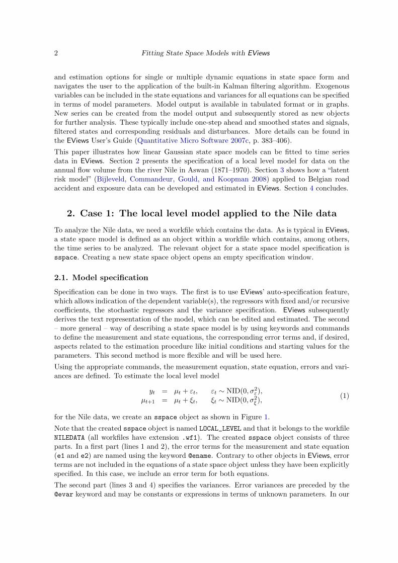
for the Nile data, we create an sspace object as shown in Figure 1.

Note that the created sspace object is named LOCAL_LEVEL and that it belongs to the workfileNILEDATA (all workfiles have extension .wf1). The created sspace object consists of threeparts. In a first part (lines 1 and 2), the error terms for the measurement and state equation(e1 and e2) are named using the keyword @ename. Contrary to other objects in EViews, errorterms are not included in the equations of a state space object unless they have been explicitlyspecified. In this case, we include an error term for both equations.

The second part (lines 3 and 4) specifies the variances. Error variances are preceded by the@evar keyword and may be constants or expressions in terms of unknown parameters. In our

Journal of Statistical Software 3

Figure 1: A state space object in EViews.

model, the variances are expressed as exponential functions of the coefficients C(1) and C(2),to guarantee nonnegative variance estimates (Quantitative Micro Software 2007c). Using the@evar command, one can also specify covariances between error terms, for example @evar

cov(e1,e2)=0.5. Variances and/or covariances that have not been specified are assumed tobe equal to zero.

In the third part (lines 5 and 6), the measurement and state equations are defined. The@signal keyword specifies the measurement equation for the dependent variable volume andincludes an unobserved level SV1 to represent µt and an observation disturbance e1 whichcorresponds to εt and has been declared in line 1. Signal equations may include expressionsof the dependent variable, but no current values or leads of signal variables. Nonlinearities inthe states and leads or lags of states are not allowed. Note that the @signal keyword maybe dropped.

The @state equation defines the random walk for the unobserved model component µt. Stateequations should not include expressions of unobserved components (like log(SV1)) nor (lagsor leads of) signal equation dependent variables, but may contain (possibly nonlinear trans-formations of) exogenous variables. They should be linear in the one-period lags of the states,where the one-period lag restriction is easily circumvented by including new state variablesfor higher order lags.

Error terms should not necessarily be named before specifying the state and observation equa-tion. One can simply add the variance structure to define an error term, like in @state SV1 =

SV1(-1) + [var=exp(C(2))]. This is called the “error variance specification” (QuantitativeMicro Software 2007c, p. 389), whereas in our program we used the “named error” approach(Quantitative Micro Software 2007c, p. 391).

The model presented above can easily be constructed using the auto-specification feature inEViews. All we need to do is set volume as the dependent variable and include a unit randomwalk coefficient.

2.2. Estimation

Once the model has been specified as shown above, the unknown parameters for the variancesand the unobserved component can be estimated. Estimation is done by maximum likelihood.The loglikelihood function in EViews (Quantitative Micro Software 2007c, p. 387) correspondsto the one given by Durbin and Koopman (2001, p. 138) and is refered to by Harvey as the“prediction error decomposition” (Harvey 1989, p. 126).

Unless stated otherwise, the starting values for the parameters C(1) and C(2) are those


Figure 2: Output of the local level model for the Nile data.

specified in the coefficient vector, which is yet another object in the EViews workfile. Ifnecessary, the starting values can be changed by the user with @param statements.

Usually, the end user should not handle the initial conditions. Whenever possible, the steadystate conditions are solved for the mean a1 and variance P1 of the initial state vector α1.Otherwise, estimation is started from a diffuse initialization. In case prior information on a1and P1 is available, the user can supply initial values by means of the @mprior and @vprior

keywords, for the mean and variance respectively.

EViews offers two first derivative methods for optimizing the loglikelihood function: Marquardtand Berndt-Hall-Hall-Hausman. The first is a modification of the Gauss-Newton algorithm,while the second builds on Newton-Raphson. EViews further allows setting the estimationsample, the maximum number of iterations and the convergence tolerance. Note the impor-tance of the starting values, whichever optimization method is used. In general, “you mayhave to experiment to find good starting values” (Quantitative Micro Software 2007c, p. 626).

2.3. Results

Figure 2 shows the estimation output for the local level model fitted to the Nile data. The out-put shows that the model has been fitted on 100 observations using the Marquardt optimiza-tion algorithm. EViews needed 155 iterations to achieve a converging solution. At convergencethe maximum of the log likelihood is found to be −645.1781. The coefficients C(1) and C(2)

are the logs of the variances of the error terms for the measurement and state equations. Wetherefore estimate that σ2ε = exp(9.6004) = 14769.9537 and σ2ξ = exp(7.3487) = 1554.1828.The final state of the unobserved component is 816.7538. The value shown in the output,795.5689, is the one-step ahead predicted value for the first out-of-sample period (Quantita-tive Micro Software 2007a, p. 428). The initial state value of the level is not reported, butcan be found in the model output to be µ1 = 1119.9989.

EViews allows creating new series based on the results of the estimation process. These can begenerated using the appropriate keywords, or they can be selected from the menu screens (seefor example the state and signal screens shown in Figure 3). Some of the generated series for


(a) “Make signal series” screen (b) “Make state series” screen

Figure 3: Creating signal and state series.

the analysis of the Nile data are summarized in Figure 4. Figure 4a shows the Nile volume dataand the smoothed state estimates together with 90% confidence bands. Figure 4b containsthe standardized prediction errors, which can be calculated from the output as the ratio ofthe prediction residuals and the prediction residuals standard errors. They can also readilybe obtained from the EViews output by asking for the “standardized prediction residuals”.Figures 4c and 4d show the auxiliary residuals for the signal and the state respectively. Theyare obtained by selecting the smoothed standardized disturbance estimates in the signal andstate results (via the proc/make signal series menu). Alternatively, they are calculatedby dividing the smoothed observation and state disturbance estimates (εt and ξt) by theircorresponding standard errors. Note that the graphs also include 95% confidence bands tocheck for outliers and structural breaks.

Once a series is generated, the usual statistical tools available in EViews can be applied. Forexample, in Figure 5 the correlogram with Box-Ljung statistics and the Jarque-Bera normalitytest for the standardized prediction errors are shown. Note, however, that these diagnosticsare not readily available and should be generated outside the sspace object. This implies thatthe sample for generating the correlogram, as well as the associated degrees of freedom, areusually incorrect. In the standard setting, the correlogram is generated using the completesample (n = 100) and the degrees of freedom in EViews are equal to the number of lags.

To be more precise, we generate the correlogram after a sample adjustment (smpl 1872 1970)and calculate the degrees of freedom as k −w + 1, where k is the number of lags in the Box-Ljung statistic and w is the number of diffuse priors (Commandeur and Koopman 2007). Forexample, for Q(10) we find a value of 13.117 for n = 99 (instead of 13.310 for n = 100).Given two disturbance variances in the model, the corresponding p value should be basedon a χ2

(10−2+1) distribution, resulting in a p value of 0.1574 (instead of 0.2172 in Figure 5a).Correcting for the number of disturbance variances renders the test slightly more conservative,in the sense that the null hypothesis of independence will be rejected more often. For thismodel, the difference in degrees of freedom is small, however, and in practice the standardoutput may be used. After sample adjustment, the Jarque-Bera test for normality can easilybe asked for (see Figure 5b: JB = 0.0417, p value = 0.9794).


400

600

800

1000

1200

1400

1875 1900 1925 1950

(a) Smoothed State and 90% CI

-3

-2

-1

0

1

2

3

1875 1900 1925 1950

(b) Standardized Prediction Errors

-4

-3

-2

-1

0

1

2

3

1875 1900 1925 1950

(c) Auxiliary residuals (signal)

-4

-3

-2

-1

0

1

2

3

1875 1900 1925 1950

(d) Auxiliary residuals (state)

Figure 4: Nile data and Kalman filter output.

(a) Correlogram

0

2

4

6

8

10

12

14

-3 -2 -1 0 1 2

Jarque-Bera 0.041686Probability 0.979373

(b) Normality test

Figure 5: Analysis of standardized prediction errors.


400

600

800

1000

1200

1400

1875 1900 1925 1950 1975

Figure 6: Forecasts and 50% confidence interval.

Finally, one-step-ahead forecasts and corresponding standard errors were generated from thesspace object for the years 1971–1980. The value of the level at t = n+ 1 is forecasted to be795.5689, and the forecast remains constant for the other years. The forecasts and the 50%confidence interval are shown in Figure 6.

3. Case 2: Fitting a latent risk model in EViews

3.1. Introduction

In this section we show how the latent risk model (Bijleveld et al. 2008) can be fitted inEViews. Apart from the model specification, an iteration program is presented that can beused to facilitate convergence of the optimization procedure.

The application presented here belongs to the domain of macroscopic road safety modeling.One objective of road safety modeling is to describe and explain long term trends in thenumber of road fatalities. The annual number of fatalities is an important indicator of the roadsafety performance of a country. Policy makers refer to it to investigate past trends in roadsafety and to set targets for future improvement. In many countries, long-term quantitativeobjectives are expressed in terms of the number of fatalities (e.g. “half the number of fatalitiesby 2010”). In Belgium, new road safety targets have been formulated in 2007, aiming at nomore than 500 fatalities in 2015.

Consider the time series in Figure 7, representing the yearly number of vehicle kilometres(Figure 7a) and the number of road fatalities (Figure 7b) in Belgium for the period 1965–2008. The number of vehicle kilometres is typically used as a measure of exposure to risk. Itis assumed that the level of exposure is one of the major factors influencing the number offatalities. In particular, if “risk” is defined as the ratio of the number of fatalities to the levelof exposure, then the number of fatalities can be expressed as the level of exposure multipliedby the level of risk, thereby disentangling the number of fatalities in its major components.


20

30

40

50

60

70

80

90

100

1970 1980 1990 2000 2010

(a) Number of vehicle kilometres (×109)

800

1200

1600

2000

2400

2800

3200

1970 1980 1990 2000 2010

(b) Number of fatalities

Figure 7: Belgian road fatalities and vehicle exposure.

However, as both exposure and risk can never be faultlessly observed, we model them bymeans of unobserved components. A precursor of this application was presented in Van denBossche (2006).

3.2. Model development

The latent risk model is a special case of the general Gaussian state space model which canbe written as:

yt = Ztαt + εt, εt ∼ NID(0, Ht),αt+1 = Ttαt +Rtηt, ηt ∼ NID(0, Qt),

(2)

for t = 1, . . . , n. The first equation is the observation equation, in which yt represents a p× 1vector containing the observed values at time t for the p dependent variables. The εt vector ofdimension (p× 1) contains the p corresponding observation disturbances. These are assumedto be NID, with zero means and a variance-covariance structure collected in the p× p matrixHt. Assuming m state components in this model, Zt is a p ×m observation matrix, and αtis the state vector of order m × 1. The transition matrix Tt is a block diagonal matrix oforder m×m. The m state disturbances are gathered in the m× 1 vector ηt. They have zeromeans and an unknown variance-covariance matrix Qt of order m×m. Finally, Rt is usuallyan identity matrix of order m × m, but it can also be a selection matrix of order m × r,with r < m, containing the first r columns of the identity matrix. For further details on theformulation of this multivariate model, see Harvey (1989), Durbin and Koopman (2001) andthe introductory article of this special volume.

To develop the latent risk model, consider a local linear trend model with two dependentvariables (p = 2), namely the observed annual exposure or mobility Mt (expressed as thenumber of vehicle kilometres driven per year) and the observed annual number of fatalitiesFt. Each observation equation is further described in two state equations, one for the leveland one for the slope (m = 4). To model the mobility and fatalities series simultaneously ina multivariate model, define the vector yt as (Bijleveld and Commandeur 2006):

yt =

(y(1)t

y(2)t

)=

(log(Mt)log(Ft)

). (3)


In addition, define the vectors αt, εt and ηt, and the matrices Tt, Rt, Zt, Ht and Qt as follows:

αt =

µ(1)t

ν(1)t

µ(2)t

ν(2)t

, ηt =

ξ(1)t

ζ(1)t

ξ(2)t

ζ(2)t

, Tt =

1 1 0 00 1 0 00 0 1 10 0 0 1

, Rt =

1 0 0 00 1 0 00 0 1 00 0 0 1

,

Zt =

[1 0 0 01 0 1 0

], εt =

[ε(1)t

ε(2)t

], Ht =

[σε(1) cov(ε

(1)t , ε

(2)t )

cov(ε(1)t , ε

(2)t ) σε(2)

],

Qt =

σ2ξ(1)

0 cov(ξ(1), ξ(2)) 0

0 σ2ζ(1)

0 cov(ζ(1), ζ(2))

cov(ξ(1), ξ(2)) 0 σ2ξ(2)

0

0 cov(ζ(1), ζ(2)) 0 σ2ζ(2)

.

(4)

These vectors and matrices completely define the latent risk model. Writing out these com-ponents in scalar notation yields the following two observation equations:

y(1)t = µ

(1)t + ε

(1)t , (5a)

y(2)t = µ

(1)t + µ

(2)t + ε

(2)t , (5b)

while the four state equations can be written as:

µ(1)t = µ

(1)t−1 + ν

(1)t−1 + ξ

(1)t , (6a)

ν(1)t = ν

(1)t−1 + ζ

(1)t , (6b)

µ(2)t = µ

(2)t−1 + ν

(2)t−1 + ξ

(2)t , (6c)

ν(2)t = ν

(2)t−1 + ζ

(2)t . (6d)

The first observation equation (5a) is for the log of the observed mobility (exposure). Equa-tions (6a) and (6b) are the corresponding state equations for the mobility trend and slopecomponents. The second observation equation (5b) represents the log of the number of fatali-ties, for which the dynamics (trend and slope) are determined by the state equations (6c) and(6d). Given the vector and matrix definitions in the equation set (4), covariances betweentrend and slope components are assumed to be zero. Covariances are estimated mutually forthe trend errors, the slope errors and the observation errors.

Given the fact that this model is linear in the logarithms, it is essentially a multiplicativemodel, representing the number of fatalities as the product of exposure and risk. This isin line with the models developed by Oppe (1989, 1991). The difference with these models,however, is that the model at hand is multivariate in nature, and that the exposure and riskcomponents are unobserved, without any assumption about their functional form. Hence the“latent risk” designation.


Figure 8: Iteration program for the latent risk model.

3.3. Iteration program

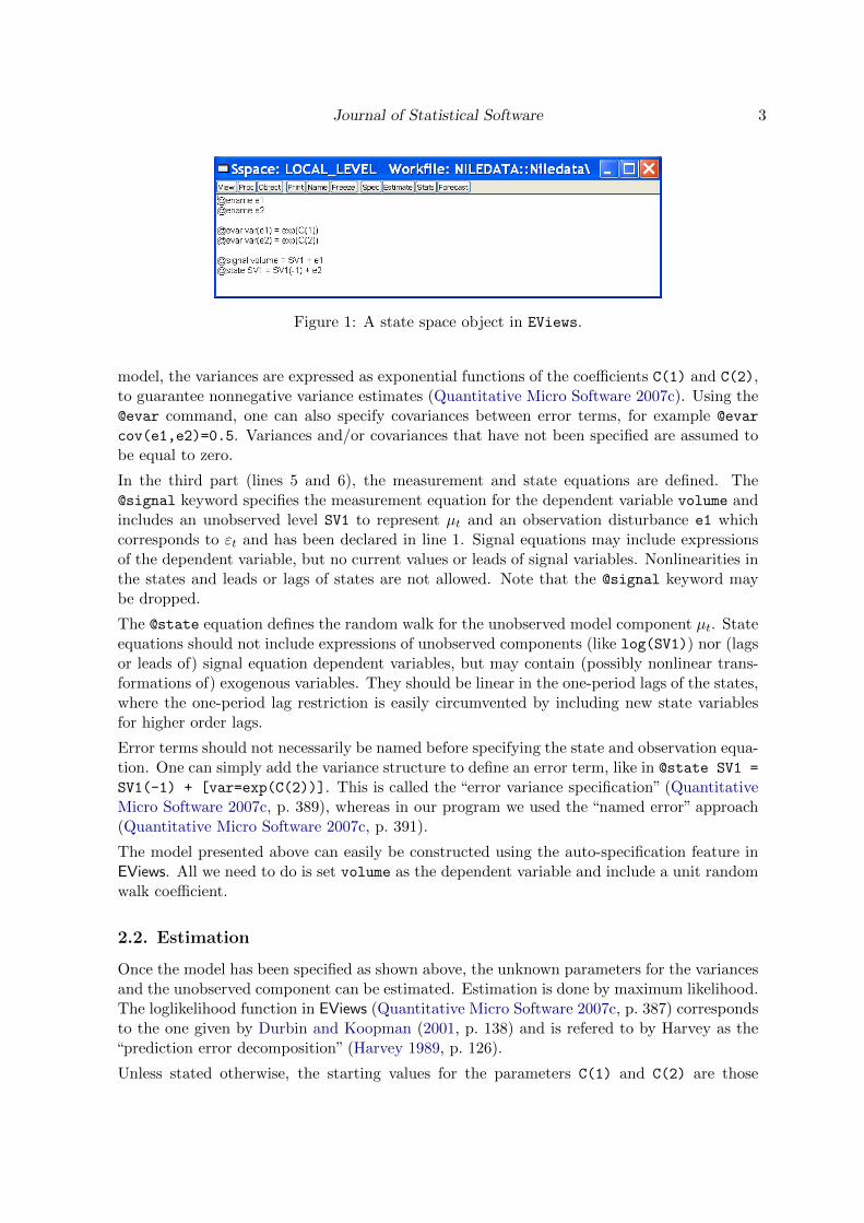
The errors and variances and the observation and state equations, as described in the previoussection, define the latent risk model. Using the Estimate button in the sspace object, thismodel can in principle be estimated. However, because of the more complex multivariatenature of the model, the optimization procedure may find a suboptimal or no solution. Todecrease the likelihood of estimation problems, a multiple random start procedure is set up,which runs the optimization algorithm repeatedly, each time starting from a different set ofinitial values for the model parameters. The program that executes these iterations is shownin Figure 8. It is an illustration of how the programming environment in EViews can be usedto support the specification and estimation of state space models. Line numbers are addedfor ease of reference, they do not belong to the program.


Preparatory declarations

The first part of the program contains declarations of variables and objects that are needed inthe remainder of the program. In line 2, a state space object solution is created. This objectwill hold the optimal solution when the iteration program finishes (see below). In line 3, avariable !loglik is declared, holding the value −1000000 at the start. This is deliberatelychosen to be a large negative value that will be overwritten by the program as soon as amodel is obtained with a loglikelihood value greater than −1000000. The loglikelihood willbe used as an indicator to compare model solutions obtained during the iteration process.Line 4 creates a table object called results. This is a table that will hold all solutions forwhich the optimization procedure converged. It contains one new row for each convergingestimation run.

The cells in the table are referred to by means of row and column numbers. Lines 5–9 createthe headings LogLik, Result, AIC, Schwarz and Hannan-Quinn in the first row. The LogLik

column will hold the loglikelihood value, and the Result column will show the number ofiterations that were necessary to obtain the solution (for example: Convergence achievedafter 31 iterations). The other headings indicate model quality statistics.

In line 10, the variable row is set equal to 1. This is a counter that will be used to appropriatelyfill the results table.

Selection of starting values

In line 11, a for-loop is used to iterate the subsequent code a number of times. In thisprogram the state space model is solved 1000 times starting from different initial parametervalues. This for-loop ends in line 71. The different steps will be explained below.

Line 12 restores the full sample to create a new series named start in line 13. We will use thisseries to select starting values for the parameters that determine the variances and covariancesin the model. The series start is based on a uniform [0, 1] random variable that is generatedby the built-in function rnd. Note that this code generates more starting values than needed(it is a series), so we will have to select as much values from this series as needed to definethe variances and covariances in the model.

In lines 14 to 17, another for-loop is executed. These lines are used to assign starting valuesto the parameters. For the latent risk model, 9 parameters are to be estimated, so the countervariable takes values 1 up to 9. The scalar !startvar picks the j-th value from the start

series, and this value is assigned to the j-th parameter in line 16. The keyword next initiatesthe next run in the for-loop that started at line 14.

In line 18, the sample for the analysis is set. This may be different from the sample size inthe data set when, for example, forecasting is required. In the program, data from 1965 upto 2008 will be used to estimate the model.

Definition of the state space program

Once the starting values for the parameters are determined, the state space object ss1 iscreated in line 19. This object will contain, in every iteration, the estimated solution of themodel. Lines 20–44 contain the state space program, using similar keywords as in Figure 1.Note the ss1.append command at the beginning of each line, that is used for adding lines tothe state space model in a program.


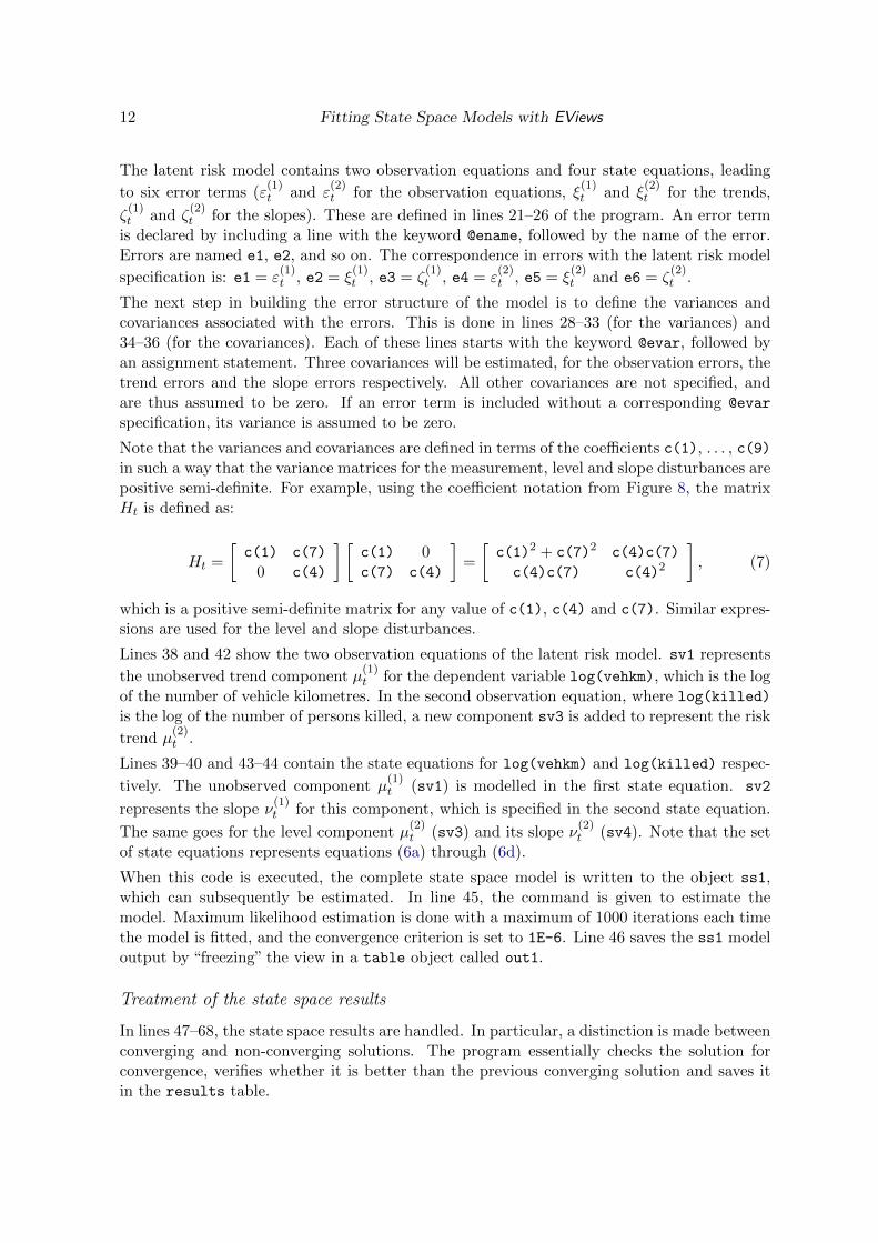
The latent risk model contains two observation equations and four state equations, leading

to six error terms (ε(1)t and ε

(2)t for the observation equations, ξ

(1)t and ξ

(2)t for the trends,

ζ(1)t and ζ

(2)t for the slopes). These are defined in lines 21–26 of the program. An error term

is declared by including a line with the keyword @ename, followed by the name of the error.Errors are named e1, e2, and so on. The correspondence in errors with the latent risk model

specification is: e1 = ε(1)t , e2 = ξ

(1)t , e3 = ζ

(1)t , e4 = ε

(2)t , e5 = ξ

(2)t and e6 = ζ

(2)t .

The next step in building the error structure of the model is to define the variances andcovariances associated with the errors. This is done in lines 28–33 (for the variances) and34–36 (for the covariances). Each of these lines starts with the keyword @evar, followed byan assignment statement. Three covariances will be estimated, for the observation errors, thetrend errors and the slope errors respectively. All other covariances are not specified, andare thus assumed to be zero. If an error term is included without a corresponding @evar

specification, its variance is assumed to be zero.

Note that the variances and covariances are defined in terms of the coefficients c(1), . . . , c(9)in such a way that the variance matrices for the measurement, level and slope disturbances arepositive semi-definite. For example, using the coefficient notation from Figure 8, the matrixHt is defined as:

Ht =

[c(1) c(7)

0 c(4)

] [c(1) 0c(7) c(4)

]=

[c(1)2 + c(7)2 c(4)c(7)

c(4)c(7) c(4)2

], (7)

which is a positive semi-definite matrix for any value of c(1), c(4) and c(7). Similar expres-sions are used for the level and slope disturbances.

Lines 38 and 42 show the two observation equations of the latent risk model. sv1 represents

the unobserved trend component µ(1)t for the dependent variable log(vehkm), which is the log

of the number of vehicle kilometres. In the second observation equation, where log(killed)

is the log of the number of persons killed, a new component sv3 is added to represent the risk

trend µ(2)t .

Lines 39–40 and 43–44 contain the state equations for log(vehkm) and log(killed) respec-

tively. The unobserved component µ(1)t (sv1) is modelled in the first state equation. sv2

represents the slope ν(1)t for this component, which is specified in the second state equation.

The same goes for the level component µ(2)t (sv3) and its slope ν

(2)t (sv4). Note that the set

of state equations represents equations (6a) through (6d).

When this code is executed, the complete state space model is written to the object ss1,which can subsequently be estimated. In line 45, the command is given to estimate themodel. Maximum likelihood estimation is done with a maximum of 1000 iterations each timethe model is fitted, and the convergence criterion is set to 1E-6. Line 46 saves the ss1 modeloutput by “freezing” the view in a table object called out1.

Treatment of the state space results

In lines 47–68, the state space results are handled. In particular, a distinction is made betweenconverging and non-converging solutions. The program essentially checks the solution forconvergence, verifies whether it is better than the previous converging solution and saves itin the results table.


In line 47, a string (%st1) is taken from the contents in the cell on row 6 and column 1 of theout1 table, which contains the convergence message. In line 48, it is assessed whether thefirst 11 characters in this cell form the word Convergence, which is the case if a valid solutionis obtained.

Once a solution is found, two steps follow: (i) the main results are written on a new line inthe table results, and (ii) the loglikelihood is checked. In addition, if the loglikelihood valueis better than the one of the previous best solution, it has to be saved. In line 49, a newrow in the table results is selected. In the first column, the log likelihood is written (line50), and the second column contains the convergence message (line 51). The next columnscontain the Akaike, Schwarz and Hannan-Quinn criteria (lines 52–54). The for-loop in lines56–58 stores the initial values for the 9 parameters, while lines 60–62 are for the final values.In line 63, it is checked whether the last loglikelihood value is better than the one previouslystored. If the most recent loglikelihood is indeed better, it is written to the variable !loglik

(line 64), and the ss1 model is copied into an object called solution (line 66). If the latterobject already exists, it is first deleted (line 65).

In lines 69–70, the temporary objects out1 and ss1 are deleted. They will be re-created inevery new run of the program. In line 71, the next iteration in the for-loop is initiated, andin line 72 the program terminates. The object solution now contains the final (best andconverging) model, and the table results shows details on all converging solutions. Note,however, that this program will not always work. The outcome is sensitive to good startingvalues. Sometimes no solution and, in rare occasions, a degenerate solution is found.

Results

As an example, the latent risk model has been fitted to the Belgian fatalities and exposuredata shown in Figure 7. In a first run, a possible level shift was noticed in 1978 for the numberof vehicle kilometres. Also, we explicitly modelled the “top” year 1970 by including a pulseintervention in the slope equation (6d) of the latent risk, and fixing the error of this equationto zero renders the slope deterministic. In combination with a pulse intervention this resultsin a piecewise linear slope component.

We adjust the counter in line 14 of the program to select starting values for 11 instead of9 parameters. We drop the error declaration for e6 (line 26), its variance (line 33) andthe covariance between e3 and e6 (line 36). Then we change line 38 to ss1.append @signal

log(vehkm) = sv1 + c(10)*level1978 + e1, where level1978 is a level shift variable thatequals 0 at all time points before 1978 and equals 1 in 1978 and subsequent years. Line 44 nowbecomes ss1.append @state sv4 = sv4(-1) + c(11)*pulse1970. Note that level1978

and pulse1970 need to be defined as new series in the work file.

The final model solution has a loglikelihood value of 137.3071 (AIC = −5.7867). The esti-mated variance-covariance matrices are as follows:

Ht =

[0.000019 −0.000064−0.000064 0.000352

],

Qt =

0.000071 0 0.0002720 0.000117 0

0.000272 0 0.002399

. (8)


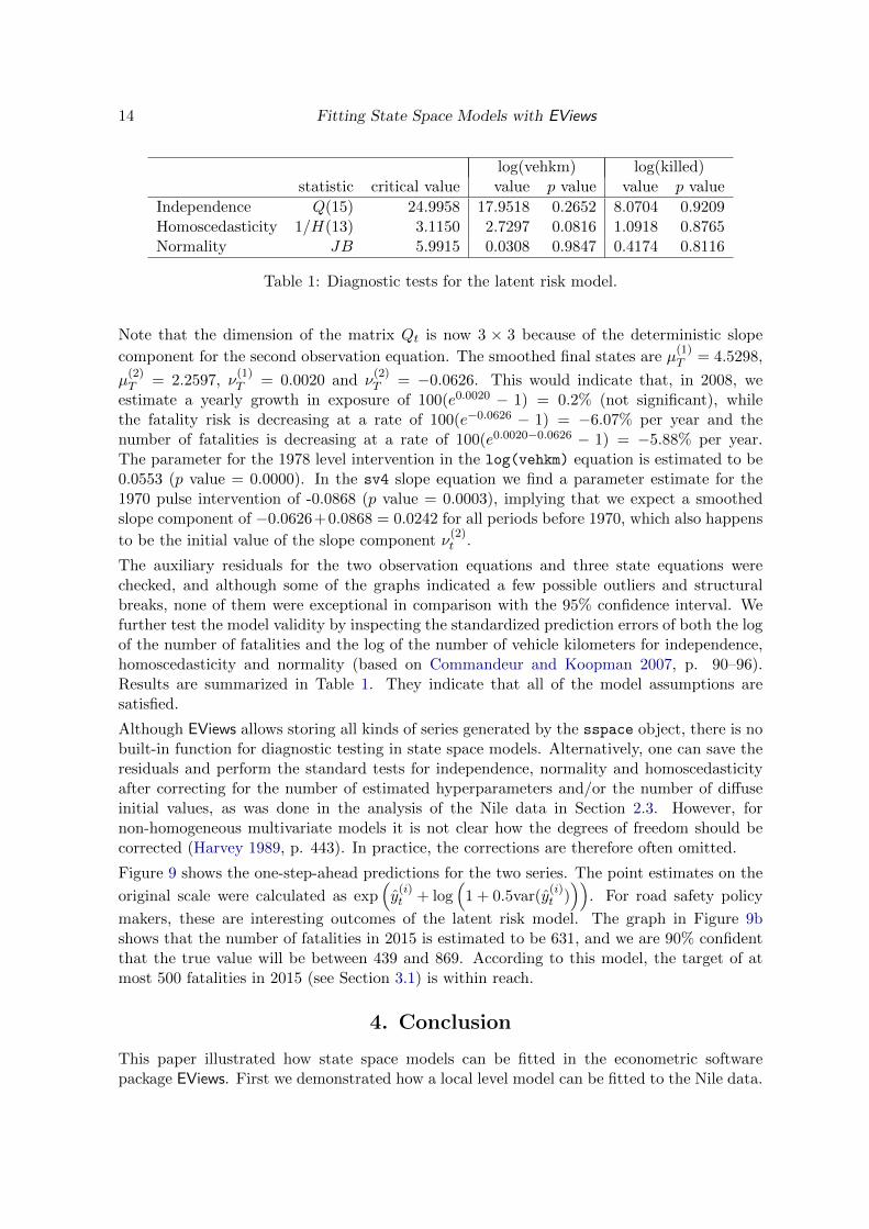
log(vehkm) log(killed)statistic critical value value p value value p value

Independence Q(15) 24.9958 17.9518 0.2652 8.0704 0.9209Homoscedasticity 1/H(13) 3.1150 2.7297 0.0816 1.0918 0.8765Normality JB 5.9915 0.0308 0.9847 0.4174 0.8116

Table 1: Diagnostic tests for the latent risk model.

Note that the dimension of the matrix Qt is now 3 × 3 because of the deterministic slope

component for the second observation equation. The smoothed final states are µ(1)T = 4.5298,

µ(2)T = 2.2597, ν

(1)T = 0.0020 and ν

(2)T = −0.0626. This would indicate that, in 2008, we

estimate a yearly growth in exposure of 100(e0.0020 − 1) = 0.2% (not significant), whilethe fatality risk is decreasing at a rate of 100(e−0.0626 − 1) = −6.07% per year and thenumber of fatalities is decreasing at a rate of 100(e0.0020−0.0626 − 1) = −5.88% per year.The parameter for the 1978 level intervention in the log(vehkm) equation is estimated to be0.0553 (p value = 0.0000). In the sv4 slope equation we find a parameter estimate for the1970 pulse intervention of -0.0868 (p value = 0.0003), implying that we expect a smoothedslope component of −0.0626+0.0868 = 0.0242 for all periods before 1970, which also happens

to be the initial value of the slope component ν(2)t .

The auxiliary residuals for the two observation equations and three state equations werechecked, and although some of the graphs indicated a few possible outliers and structuralbreaks, none of them were exceptional in comparison with the 95% confidence interval. Wefurther test the model validity by inspecting the standardized prediction errors of both the logof the number of fatalities and the log of the number of vehicle kilometers for independence,homoscedasticity and normality (based on Commandeur and Koopman 2007, p. 90–96).Results are summarized in Table 1. They indicate that all of the model assumptions aresatisfied.

Although EViews allows storing all kinds of series generated by the sspace object, there is nobuilt-in function for diagnostic testing in state space models. Alternatively, one can save theresiduals and perform the standard tests for independence, normality and homoscedasticityafter correcting for the number of estimated hyperparameters and/or the number of diffuseinitial values, as was done in the analysis of the Nile data in Section 2.3. However, fornon-homogeneous multivariate models it is not clear how the degrees of freedom should becorrected (Harvey 1989, p. 443). In practice, the corrections are therefore often omitted.

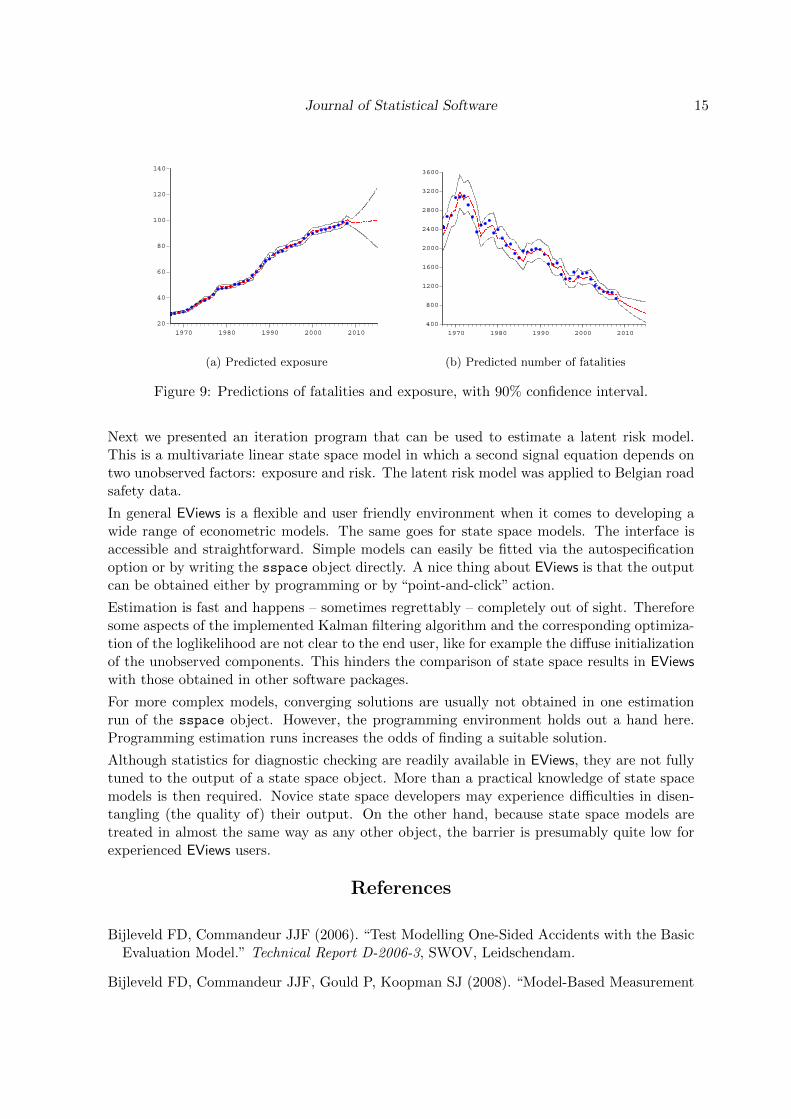
Figure 9 shows the one-step-ahead predictions for the two series. The point estimates on the

original scale were calculated as exp(y(i)t + log

(1 + 0.5var(y

(i)t )))

. For road safety policy

makers, these are interesting outcomes of the latent risk model. The graph in Figure 9bshows that the number of fatalities in 2015 is estimated to be 631, and we are 90% confidentthat the true value will be between 439 and 869. According to this model, the target of atmost 500 fatalities in 2015 (see Section 3.1) is within reach.

4. Conclusion

This paper illustrated how state space models can be fitted in the econometric softwarepackage EViews. First we demonstrated how a local level model can be fitted to the Nile data.


20

40

60

80

100

120

140

1970 1980 1990 2000 2010

(a) Predicted exposure

400

800

1200

1600

2000

2400

2800

3200

3600

1970 1980 1990 2000 2010

(b) Predicted number of fatalities

Figure 9: Predictions of fatalities and exposure, with 90% confidence interval.

Next we presented an iteration program that can be used to estimate a latent risk model.This is a multivariate linear state space model in which a second signal equation depends ontwo unobserved factors: exposure and risk. The latent risk model was applied to Belgian roadsafety data.

In general EViews is a flexible and user friendly environment when it comes to developing awide range of econometric models. The same goes for state space models. The interface isaccessible and straightforward. Simple models can easily be fitted via the autospecificationoption or by writing the sspace object directly. A nice thing about EViews is that the outputcan be obtained either by programming or by “point-and-click” action.

Estimation is fast and happens – sometimes regrettably – completely out of sight. Thereforesome aspects of the implemented Kalman filtering algorithm and the corresponding optimiza-tion of the loglikelihood are not clear to the end user, like for example the diffuse initializationof the unobserved components. This hinders the comparison of state space results in EViewswith those obtained in other software packages.

For more complex models, converging solutions are usually not obtained in one estimationrun of the sspace object. However, the programming environment holds out a hand here.Programming estimation runs increases the odds of finding a suitable solution.

Although statistics for diagnostic checking are readily available in EViews, they are not fullytuned to the output of a state space object. More than a practical knowledge of state spacemodels is then required. Novice state space developers may experience difficulties in disen-tangling (the quality of) their output. On the other hand, because state space models aretreated in almost the same way as any other object, the barrier is presumably quite low forexperienced EViews users.

References

Bijleveld FD, Commandeur JJF (2006). “Test Modelling One-Sided Accidents with the BasicEvaluation Model.” Technical Report D-2006-3, SWOV, Leidschendam.

Bijleveld FD, Commandeur JJF, Gould P, Koopman SJ (2008). “Model-Based Measurement


of Latent Risk in Time Series with Applications.” Journal of the Royal Statistical SocietyA, 171(1), 265–277.

Commandeur JJF, Koopman SJ (2007). An Introduction to State Space Time Series Analysis.Practical Econometrics. Oxford University Press, Oxford.

Durbin J, Koopman SJ (2001). Time Series Analysis by State Space Methods. Oxford Uni-versity Press, Oxford.

Harvey AC (1989). Forecasting, Structural Time Series Models and the Kalman Filter. Cam-bridge University Press, Cambridge.

Oppe S (1989). “Macroscopic Models for Traffic and Traffic Safety.” Accident Analysis andPrevention, 21, 225–232.

Oppe S (1991). “The Development of Traffic and Traffic Safety in Six Developed Countries.”Accident Analysis and Prevention, 23(5), 401–412.

Quantitative Micro Software (2007a). EViews 6 Command Reference. Irvine CA, USA. URLhttp://www.eviews.com.

Quantitative Micro Software (2007b). EViews 6 User’s Guide I. Irvine CA, USA. URLhttp://www.eviews.com.

Quantitative Micro Software (2007c). EViews 6 User’s Guide II. Irvine CA, USA. URLhttp://www.eviews.com.

Van den Bossche F (2006). Road Safety, Risk and Exposure in Belgium: An EconometricApproach. Ph.D. thesis, Hasselt University, Belgium.

Affiliation:

Filip A. M. Van den BosscheHogeschool-Universiteit BrusselFaculty of Economics and ManagementStormstraat 2BE-1000 Brussels, BelgiumandKatholieke Universiteit LeuvenFaculty of Business and EconomicsNaamsestraat 69BE-3000 Leuven, BelgiumE-mail: [email protected]

Journal of Statistical Software http://www.jstatsoft.org/

published by the American Statistical Association http://www.amstat.org/

Volume 41, Issue 8 Submitted: 2010-02-07May 2011 Accepted: 2010-12-08

http://www.eviews.com



mailto:[email protected]

http://www.jstatsoft.org/

http://www.amstat.org/

fitting state space models with eviews

Documents