fitting models to data, generalized linear least squares...
TRANSCRIPT
Fitting Models to Data,Generalized Linear Least Squares, and Error Analysis
CEE 629. System Identification
Duke University, Spring 2019
In engineering and the sciences is often of use to fit a model to measured data, in orderto predict behaviors of the modeled system, to understand how measurement errors affect theconfidence in model parameters, and to quantify the confidence in the predictive capabilitiesof the model.
This hand-out addresses the errors in parameters estimated from fitting a function todata. All samples of measured data include some amount of measurement error and somenatural variability. Results from calculations based on measured data will also depend, inpart, on random measurement errors. In other words, the normal variation in measured datapropagates through calculations applied to the data.
Many (many) quantities can not be measured directly, but can be inferred from mea-surements: gravitational acceleration, the universal gravitational constant, seasonal rainfallinto a watershed, the resistivity of a material, the elasticity of a material, metabolic rates,etc. etc. ... For example, the Earth’s gravitational acceleration can be estimated from mea-surements of the time it takes for a mass to fall from rest through a measured distance. Theequation is d = gt2/2 or g = 2dt−2. The ruler we use to measure the distance d will have afinite resolution and may also produce systematic errors if we do not account for issues suchas thermal expansion. The clock we use to measure the time t will also have some error.Fortunately, the errors associated with the ruler are in no way related to the errors in theclock. Not only are they uncorrelated they are statistically independent. If we repeat theexperiment n times, with a very precise clock, we will naturally find that measurements ofthe time ti are never repeated exactly. The variability within our sample of measurements ofd and t will surely lead to variability in the estimation of g. As described in the next section,error propagation formulas help us determine the variability of g based upon the variabilityof the measurements of d and t.
This document reviews methods for estimating model parameters and their uncertain-ties. In so doing, each individual measurement is considered to be a random variable, in whichthe randomness of the variable represents the measurement error. It is reasonable (and some-times extremely convenient) to assume that these variables are normally distributed. It isoften necessary to assume that the measurement error in one measurement is statisticallyindependent of the measurement error in all other measurements.
Estimates of the constants (i.e., fit parameters) in an equation that passes through somedata points is a function of the random sample of data. So this document starts by consideringthe statistics (mean, standard deviation) of a function of several random variables. Whenreading this, think of the function as representing the coefficients in the curve-fit, and theset of random variables as the sample of measured data.
2 CEE 690 , ME 555 – System Identification – Duke University – Spring 2019 – H.P. Gavin
1 Quadrature Error PropagationGiven a function of several random variables, F (Z1, Z2, Z3, · · · , Zn), known variations
in the independent variables, δZ1, · · · , δZn will result in a computable variation δF . Forsmall variations in Zi we can expand the variation in F in terms of individual variations ofZi using a first-order Taylor series and the chain rule of calculus,
δF = ∂F
∂Z1δZ1 + ∂F
∂Z2δZ2 + · · ·+ ∂F
∂ZnδZn. (1)
={∂F
∂Z1
∂F
∂Z2· · · ∂F
∂Zn
}· {δZ1 δZ2 · · · δZn}
= ∇F · δZ
The notation “∇F” represents the set of derivatives of F with respect to Z1, · · · , Zn andis called the gradient of F with respect to Z1, Z2, ..., Zn. When working with a sample ofmeasured data, we can not know the values of the individual measurement errors (by thedefinition of a measurement error). We can’t even know if the error in a measurement ispositive or negative. But we can usually be satisfied by estimating only the magnitude oferror in F , and not the sign. To do so we can estimate the square of δF . Note that thevariation δF is a weighted sum of the individual measurement errors δZi. Assuming that themeasurement errors are independent (at least for the time being) we can estimate the squareof δF as
(δF )2 =(∂F
∂Z1δZ1
)2
+(∂F
∂Z2δZ2
)2
+ · · ·+(∂F
∂ZnδZn
)2
. (2)
Indeed, the variance of the function is computed analogously,
σ2F =
(∂F
∂Z1
)2
σ2Z1 +
(∂F
∂Z2
)2
σ2Z2 + · · ·+
(∂F
∂Zn
)2
σ2Zn
=m∑i=1
(∂F
∂Zi
)2
σ2Zi
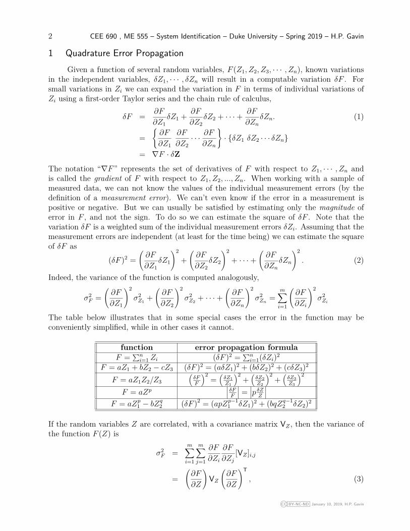
The table below illustrates that in some special cases the error in the function may beconveniently simplified, while in other cases it cannot.
function error propagation formulaF = ∑n
i=1 Zi (δF )2 = ∑ni=1(δZi)2
F = aZ1 + bZ2 − cZ3 (δF )2 = (aδZ1)2 + (bδZ2)2 + (cδZ3)2
F = aZ1Z2/Z3(δFF
)2=(δZ1Z1
)2+(δZ2Z2
)2+(δZ3Z3
)2
F = aZp∣∣∣ δFF
∣∣∣ =∣∣∣p δZ
Z
∣∣∣F = aZp
1 − bZq2 (δF )2 = (apZp−1
1 δZ1)2 + (bqZq−12 δZ2)2
If the random variables Z are correlated, with a covariance matrix VZ , then the variance ofthe function F (Z) is
σ2F =
m∑i=1
m∑j=1
∂F
∂Zi
∂F
∂Zj[VZ ]i,j
=(∂F
∂Z
)VZ
(∂F
∂Z
)T
, (3)
CC BY-NC-ND January 10, 2019, H.P. Gavin
Linear Least Squares 3
where (∂F/∂Z) is the m-dimensional row-vector of the gradient of F with respect to Z, and[VZ ]i,i = σ2
Zi. Finally, if F (Z) is an m-dimensional vector-valued function of n correlated
random variables, with covariance matrix VZ , then the m×m covariance matrix of F is
[VF ]k,l =n∑i=1
n∑j=1
∂Fk∂Zi
∂Fl∂Zj
[VZ ]i,j
VF =[∂F
∂Z
]VZ
[∂F
∂Z
]T
. (4)
where [∂F/∂Z] is an m × n matrix and is called the Jacobian of F with respect to Z. TheJacobian quantifies the sensitivity of each element Fk to each Zi individually,[
∂F
∂Z
]k,i
= ∂Fk∂Zi
, (5)
and the covariance quantifies the variability amongst the data. Equation (4) shows how thesensitivities of a function to its variables and the variability amongst the variables themselvesare combined in order to estimate the variability of the function. It is centrally important towhat follows.
2 An Example of Linear Least SquaresMeasured data are often used to estimate values for the parameters of a model (or the
coefficients in an equation). Consider the fitting of a function y(x; a) that involves a set ofcoefficients a1, ...an, to a set of m measured data points (xi, yi), i = 1, ...,m. If the functionis linear in the coefficients then the relationship between the data and the coefficients canalways be written as a matrix-vector product
y(x; a) = Xa
where
• a is the vector of the coefficients to be estimated.
• y(x; a) is the function to be fit to the m data coordinates (yi, xi), and
• the matrix X depends only on the set of independent variables, x.
As a general example, consider the problem of fitting an (n− 1) degree power-polynomial tom measured data coordinates, (xi, yi), i = 1, · · · ,m. The general form of the equation is
y(x; a) = a0 + a1x+ a2x2 + · · ·+ an−1x
n−1, (6)
The equation may be written m times for every data coordinate (xi, yi), i = 1, · · · ,m,
y1(x, a) = a0 + a1x1 + a2x21+ · · ·+ an−1x
n−11
y2(x, a) = a0 + a1x2 + a2x22+ · · ·+ an−1x
n−12
... . . .ym(x, a) = a0 + a1xm + a2x
2m+ · · ·+ an−1x
n−1m
CC BY-NC-ND January 10, 2019, H.P. Gavin
4 CEE 690 , ME 555 – System Identification – Duke University – Spring 2019 – H.P. Gavin
or, in matrix form as y(x; a) = Xa,
y1y2...ym
=
1 x1 x2
1 · · · xn−11
1 x2 x22 · · · xn−1
2... ... ... . . . ...1 xm x2
m · · · xn−1m
a0a1a2...
an−1
. (7)
Matrices structured in the form of X in equation (7) are called vanderMonde and arise incuve-fitting problems. The number of parameters (n in this example) must always be lessthan or equal to the number of data coordinates, m. We can assume that each measurementyi has a particular variance, σ2
yi, and, unless we know better, we should further assume that
the sample of measurements yi are uncorrelated.
Fitting the equation to the data reduces to estimating values of n parameters, a0, · · · , an−1such that the equation represents the data as closely as possible.
But what does “as closely as possible” even mean?
In 1829 Carl Friedrich Gauss proved that it is physically sound and mathematicallyconvenient to say that the best-fit minimizes the sum of the squares of the errors betweenthe data and the model regression. So to find estimates for the parameters, we would liketo minimize the sum of the squares of the residual errors ri between the data, yi, and theequation, y(xi; a).
ri = y(xi; a)− yi.Furthermore, the error should be more heavily weighted with the high-accuracy (small-variance) data and less heavily weighted with the low-accuracy (large-variance) data. Thisfit criterion is called the weighted sum of the squared residuals (WSSR), also called the ‘chi-squared’ error function,
χ2(a) =m∑i=1
[y(xi; a)− yi]2 /σ2yi
(8)
An equivalent expression for χ2(a) may be written in terms of the vectors y and a, the systemmatrix X, and the data covariance matrix Vy
χ2(a) = {Xa− y}T V−1y {Xa− y},
= aTXT V−1y Xa− 2aTXT V−1
y y + yT V−1y y. (9)
Prove to yourself that if Vy is the diagonal matrix of variances of y, σ2yi
, then equation (9) isequivalent to equation (8). If the data covariance matrix is not diagonal, then equation (9)is a generalization of (8).
Note that any weighted least squares problem can be scaled to an unweighted leastsquares problem as long as the weighting matrix is symmetric and positive-definite. Decom-posing the weighting matrix into Cholesky factors, V−1
y = RTR, and defining y = Ry andX = RX, any weighted criterion (9) is equivalent to the unweighted criterion, with no lossof generality.
χ2(a) = {Xa− y}T{Xa− y} .
CC BY-NC-ND January 10, 2019, H.P. Gavin
Linear Least Squares 5
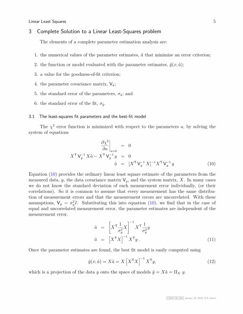
3 Complete Solution to a Linear Least-Squares problem
The elements of a complete parameter estimation analysis are:
1. the numerical values of the parameter estimates, a that minimize an error criterion;
2. the function or model evaluated with the parameter estimates, y(x; a);
3. a value for the goodness-of-fit criterion;
4. the parameter covariance matrix, Va;
5. the standard error of the parameters, σa; and
6. the standard error of the fit, σy.
3.1 The least-squares fit parameters and the best-fit model
The χ2 error function is minimized with respect to the parameters a, by solving thesystem of equations
∂χ2
∂a
∣∣∣∣∣a=a
= 0
XT V−1y Xa−XT V−1
y y = 0a = [XT V−1
y X]−1XT V−1y y (10)
Equation (10) provides the ordinary linear least square estimate of the parameters from themeasured data, y, the data covariance matrix Vy, and the system matrix, X. In many caseswe do not know the standard deviation of each measurement error individually, (or theircorrelations). So it is common to assume that every measurement has the same distribu-tion of measurement errors and that the measurement errors are uncorrelated. With theseassumptions, Vy = σ2
yI. Substituting this into equation (10), we find that in the case ofequal and uncorrelated measurement error, the parameter estimates are independent of themeasurement error.
a =[XT 1
σ2y
X
]−1
XT 1σ2y
y
a =[XTX
]−1XTy . (11)
Once the parameter estimates are found, the best fit model is easily computed using
y(x; a) = Xa = X[XTX
]−1XTy, (12)
which is a projection of the data y onto the space of models y = Xa = ΠX y.
CC BY-NC-ND January 10, 2019, H.P. Gavin

6 CEE 690 , ME 555 – System Identification – Duke University – Spring 2019 – H.P. Gavin
3.2 Goodness of fit
Because χ2 is the error criterion, the value of χ2 quantifies of the quality of the fit. Thevalue of χ2 can be normalized to a value that is more broadly meaningful. The unbiasedestimate of the variance of the weighted residuals is χ2/(m − n + 1). In the absence of anyother information on the variance of the data, Vy, χ2 can be computed without weightingthe residuals, i.e., using σyi
= 1. In this case the variance of the measurement error can beestimated as the variance of the unweighted residuals,
σ2y = χ2
m− n+ 1 , (13)
where m is the number of measurement values and n is the number of parameters. Thisestimate of the variance of the residuals can be interpreted as the measurement error if theresulting residuals are Gaussian and uncorrelated.
The R2 goodness-of-fit criterion compares the variability in the measurements not ex-plained by the model to the total variability in the measurements.
R2 = 1−∑[yi − y(xi; a]2∑[yi − y]2 , (14)
where y is the average value of the measured data values. The R2 criterion is the ratio ofthe variability in the data that is not explained by the model to the total variability in thedata. A value of R2 = 0 means that the model does not explain the measurement variabilityany better than the mean measurement value; a negative value of R2 means that the modelexplains the measurement variability worse than the mean measurement value, and a valueof R2 = 1 means that all of the variability in the data is fully explained by the model, i.e.,there is no unexplained measurement variability.
3.3 The Covariance and standard error of the parameters
The covariance matrix of the parameter estimates, Va, is a direct application of equation(4)
Va =[∂a
∂y
]Vy
[∂a
∂y
]T
= [XT V−1y X]−1XT V−1
y Vy V−1y X[XT V−1
y X]−1
= [XT V−1y X]−1[XT V−1
y X][XT V−1y X]−1
= [XT V−1y X]−1 . (15)
This covariance matrix is sometimes called the error propagation matrix, as it indicateshow random measurement errors in the data y, as described by Vy, propagate to the modelcoefficients a. If no prior information regarding the measurement error covariance is available,and χ2 is computed without weighting the residuals, then the parameter covariance matrixmay be calculated from the expression
Va = χ2
m− n[XTX]−1 . (16)
CC BY-NC-ND January 10, 2019, H.P. Gavin
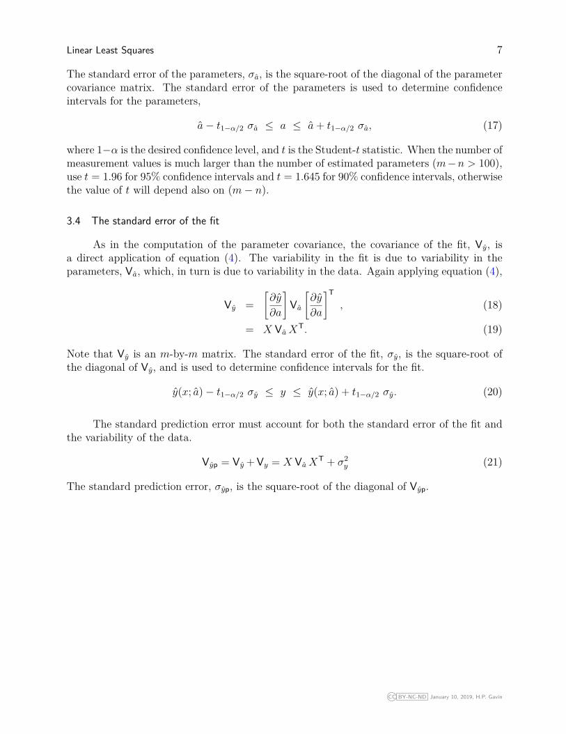
Linear Least Squares 7
The standard error of the parameters, σa, is the square-root of the diagonal of the parametercovariance matrix. The standard error of the parameters is used to determine confidenceintervals for the parameters,
a− t1−α/2 σa ≤ a ≤ a+ t1−α/2 σa, (17)
where 1−α is the desired confidence level, and t is the Student-t statistic. When the number ofmeasurement values is much larger than the number of estimated parameters (m−n > 100),use t = 1.96 for 95% confidence intervals and t = 1.645 for 90% confidence intervals, otherwisethe value of t will depend also on (m− n).
3.4 The standard error of the fit
As in the computation of the parameter covariance, the covariance of the fit, Vy, isa direct application of equation (4). The variability in the fit is due to variability in theparameters, Va, which, in turn is due to variability in the data. Again applying equation (4),
Vy =[∂y
∂a
]Va
[∂y
∂a
]T
, (18)
= X VaXT. (19)
Note that Vy is an m-by-m matrix. The standard error of the fit, σy, is the square-root ofthe diagonal of Vy, and is used to determine confidence intervals for the fit.
y(x; a)− t1−α/2 σy ≤ y ≤ y(x; a) + t1−α/2 σy. (20)
The standard prediction error must account for both the standard error of the fit andthe variability of the data.
Vyp = Vy + Vy = X VaXT + σ2
y (21)
The standard prediction error, σyp, is the square-root of the diagonal of Vyp.
CC BY-NC-ND January 10, 2019, H.P. Gavin
8 CEE 690 , ME 555 – System Identification – Duke University – Spring 2019 – H.P. Gavin
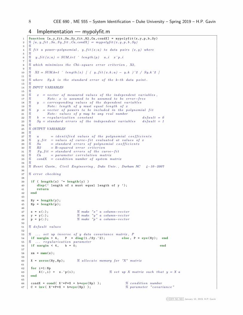
4 Implementation — mypolyfit.m1 function [a,y_fit ,Sa ,Sy_fit ,R2 ,Ca , condX ] = mypolyfit (x,y,p,b,Sy)2 % [ a , y f i t , Sa , S y f i t , Ca , condX ] = m y p o l y f i t ( x , y , p , b , Sy )3 %4 % f i t a power−polynomial , y f i t ( x ; a ) to data p a i r s ( x , y ) where5 %6 % y f i t ( x ; a ) = SUM i=1 ˆ l e n g t h ( p ) a i xˆ p i7 %8 % which minimizes the Chi−square error c r i t e r i o n , X2,9 %
10 % X2 = SUM k=1 ˆ l e n g t h ( x ) [ ( y f i t ( x k ; a ) − y k )ˆ2 / Sy k ˆ2 ]11 %12 % where Sy k i s the standard error o f the k−th data po in t .13 %14 % INPUT VARIABLES15 %16 % x = v e c t or o f measured v a l u e s o f the independent v a r i a b l e s ,17 % Note : x i s assumed to be assumed to be error−f r e e18 % y = corresponding v a l u e s o f the dependent v a r i a b l e s19 % Note : l e n g t h o f y must equa l l e n g t h o f x20 % p = v e c t o r o f powers to be inc luded in the polynomial f i t21 % Note : v a l u e s o f p may be any r e a l number22 % b = r e g u l a r i z a t i o n constant d e f a u l t = 023 % Sy = standard e rr o r s o f the independent v a r i a b l e s d e f a u l t = 124 %25 % OUTPUT VARIABLES26 %27 % a = i d e n t i f i e d v a l u e s o f the polynomial c o e f f i c i e n t s28 % y f i t = v a l u e s o f curve− f i t e v a l ua t ed at v a l u e s o f x29 % Sa = standard e r r o r s o f polynomial c o e f f i c i e n t s30 % R2 = R−squared error c r i t e r i o n31 % S y f i t = standard e r r o r s o f the curve− f i t32 % Ca = parameter c o r r e l a t i o n matrix33 % condX = cond i t i on number o f system matrix34 %35 % Henri Gavin , C i v i l Engineering , Duke Univ . , Durham NC 4−10−20073637 % error check ing3839 i f ( length(x) ˜= length(y) )40 disp(’ length of x must equal length of y ’);41 return42 end4344 Ny = length(y);45 Np = length(p);4647 x = x(:); % make ”x” a column−v e c t or48 y = y(:); % make ”y” a column−v e c t or49 p = p(:); % make ”p” a column−v e c t or5051 % d e f a u l t v a l u e s5253 % . . . s e t up i n v e r s e o f y data covar iance matrix , P54 i f nargin > 4, P = diag (1./ Sy .ˆ2); else , P = eye(Ny ); end55 % . . . r e g u l a r i z a t i o n parameter56 i f nargin < 4, b = 0; end5758 xm = max(x);5960 X = zeros(Ny ,Np ); % a l l o c a t e memory f o r ”X” matrix6162 for i=1: Np63 X(:,i) = x.ˆp(i); % s e t up X matrix such t h a t y = X a64 end6566 condX = cond( X ’*P*X + b*eye(Np) ); % cond i t ion number67 C = inv( X ’*P*X + b*eye(Np) ); % parameter ” covar iance ”
CC BY-NC-ND January 10, 2019, H.P. Gavin
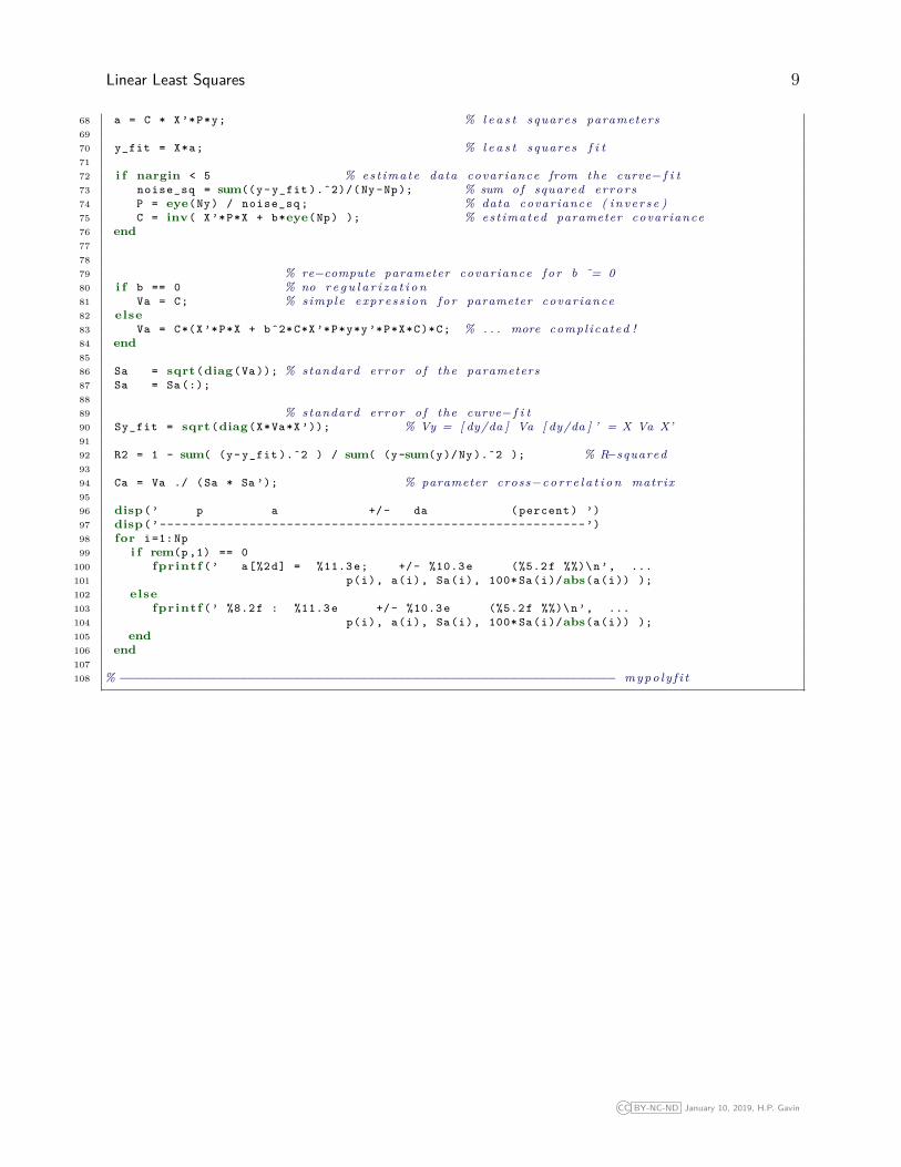
Linear Least Squares 9
68 a = C * X ’*P*y; % l e a s t squares parameters6970 y_fit = X*a; % l e a s t squares f i t7172 i f nargin < 5 % est imate data covar iance from the curve− f i t73 noise_sq = sum((y- y_fit ).ˆ2)/( Ny -Np ); % sum of squared e r r o r s74 P = eye(Ny) / noise_sq ; % data covar iance ( i n v e r s e )75 C = inv( X ’*P*X + b*eye(Np) ); % est imated parameter covar iance76 end777879 % re−compute parameter covar iance f o r b ˜= 080 i f b == 0 % no r e g u l a r i z a t i o n81 Va = C; % simple expres s ion f o r parameter covar iance82 else83 Va = C*(X ’*P*X + bˆ2*C*X ’*P*y*y ’*P*X*C)*C; % . . . more compl icated !84 end8586 Sa = sqrt (diag(Va )); % standard error o f the parameters87 Sa = Sa (:);8889 % standard error o f the curve− f i t90 Sy_fit = sqrt (diag(X*Va*X ’)); % Vy = [ dy/da ] Va [ dy/da ] ’ = X Va X’9192 R2 = 1 - sum( (y- y_fit ).ˆ2 ) / sum( (y-sum(y)/ Ny ).ˆ2 ); % R−squared9394 Ca = Va ./ (Sa * Sa ’); % parameter cross−c o r r e l a t i o n matrix9596 disp(’ p a +/- da ( percent ) ’)97 disp(’ ---------------------------------------------------------’)98 for i=1: Np99 i f rem(p ,1) == 0
100 fpr intf (’ a[%2d] = %11.3 e; +/- %10.3 e (%5.2 f %%)\n’, ...101 p(i), a(i), Sa(i), 100* Sa(i)/abs(a(i)) );102 else103 fpr intf (’ %8.2f : %11.3 e +/- %10.3 e (%5.2 f %%)\n’, ...104 p(i), a(i), Sa(i), 100* Sa(i)/abs(a(i)) );105 end106 end107108 % −−−−−−−−−−−−−−−−−−−−−−−−−−−−−−−−−−−−−−−−−−−−−−−−−−−−−−−−−−−−−−−−−− m y p o l y f i t
CC BY-NC-ND January 10, 2019, H.P. Gavin
10 CEE 690 , ME 555 – System Identification – Duke University – Spring 2019 – H.P. Gavin
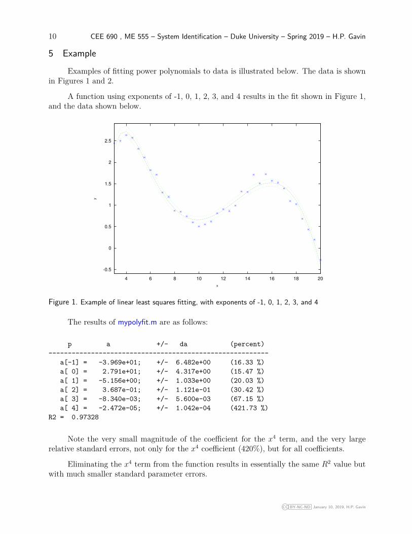
5 Example
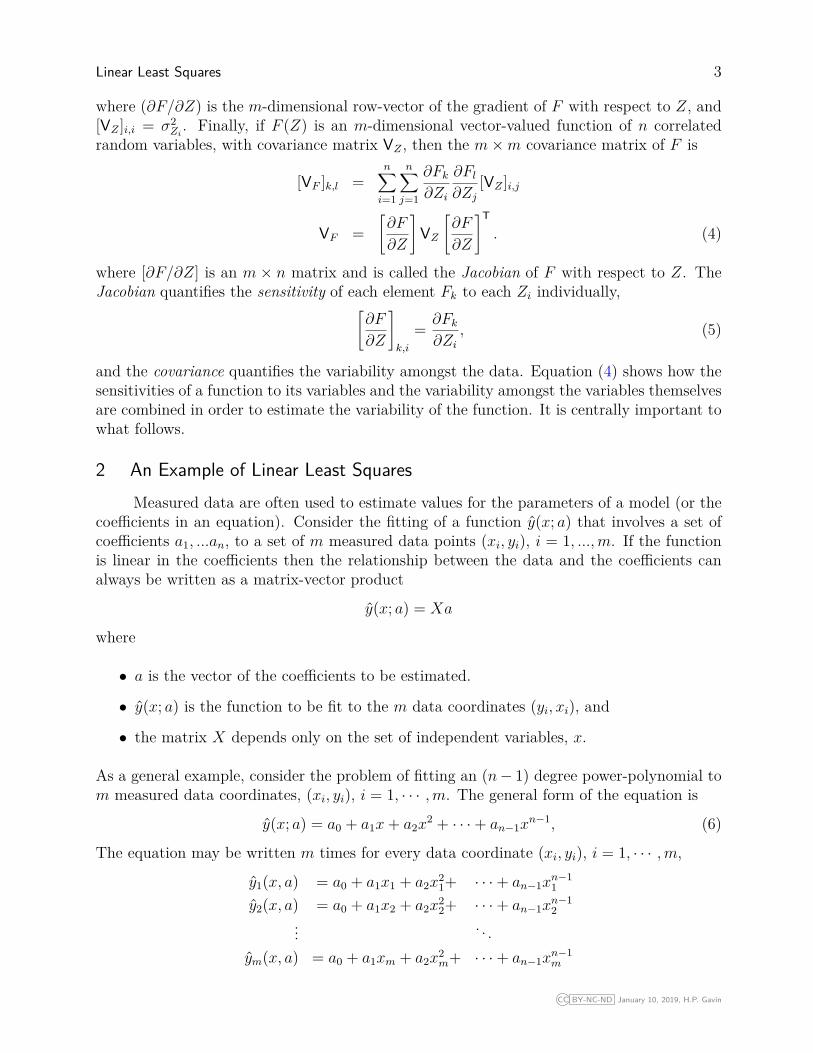
Examples of fitting power polynomials to data is illustrated below. The data is shownin Figures 1 and 2.
A function using exponents of -1, 0, 1, 2, 3, and 4 results in the fit shown in Figure 1,and the data shown below.
-0.5
0
0.5
1
1.5
2
2.5
4 6 8 10 12 14 16 18 20
y
x
Figure 1. Example of linear least squares fitting, with exponents of -1, 0, 1, 2, 3, and 4
The results of mypolyfit.m are as follows:
p a +/- da (percent)---------------------------------------------------------
a[-1] = -3.969e+01; +/- 6.482e+00 (16.33 %)a[ 0] = 2.791e+01; +/- 4.317e+00 (15.47 %)a[ 1] = -5.156e+00; +/- 1.033e+00 (20.03 %)a[ 2] = 3.687e-01; +/- 1.121e-01 (30.42 %)a[ 3] = -8.340e-03; +/- 5.600e-03 (67.15 %)a[ 4] = -2.472e-05; +/- 1.042e-04 (421.73 %)
R2 = 0.97328
Note the very small magnitude of the coefficient for the x4 term, and the very largerelative standard errors, not only for the x4 coefficient (420%), but for all coefficients.
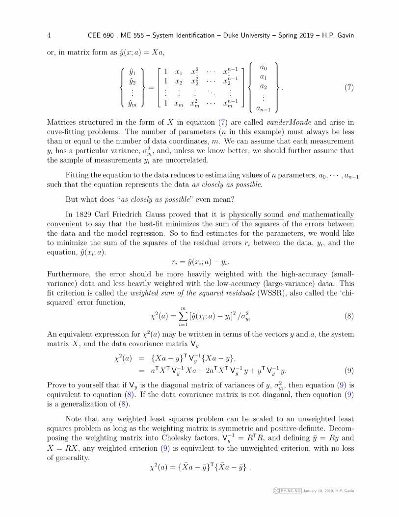
Eliminating the x4 term from the function results in essentially the same R2 value butwith much smaller standard parameter errors.
CC BY-NC-ND January 10, 2019, H.P. Gavin
Linear Least Squares 11
-0.5
0
0.5
1
1.5
2
2.5
4 6 8 10 12 14 16 18 20
y
x
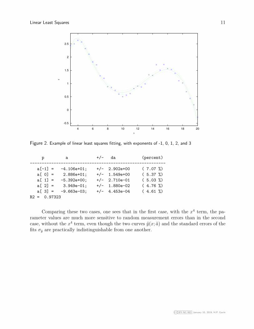
Figure 2. Example of linear least squares fitting, with exponents of -1, 0, 1, 2, and 3
p a +/- da (percent)---------------------------------------------------------
a[-1] = -4.106e+01; +/- 2.902e+00 ( 7.07 %)a[ 0] = 2.886e+01; +/- 1.549e+00 ( 5.37 %)a[ 1] = -5.392e+00; +/- 2.710e-01 ( 5.03 %)a[ 2] = 3.949e-01; +/- 1.880e-02 ( 4.76 %)a[ 3] = -9.663e-03; +/- 4.453e-04 ( 4.61 %)
R2 = 0.97323
Comparing these two cases, one sees that in the first case, with the x4 term, the pa-rameter values are much more sensitive to random measurement errors than in the secondcase, without the x4 term, even though the two curves y(x; a) and the standard errors of thefits σy are practically indistinguishable from one another.
CC BY-NC-ND January 10, 2019, H.P. Gavin
12 CEE 690 , ME 555 – System Identification – Duke University – Spring 2019 – H.P. Gavin
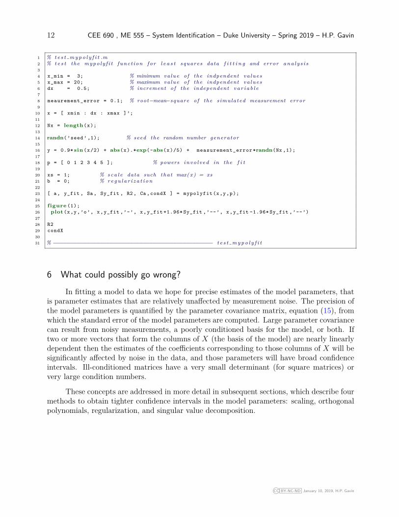
1 % t e s t m y p o l y f i t .m2 % t e s t the m y p o l y f i t f unc t i on f o r l e a s t squares data f i t t i n g and error a n a l y s i s34 x_min = 3; % minimum va lue o f the indpendent v a l u e s5 x_max = 20; % maximum va lue o f the indpendent v a l u e s6 dx = 0.5; % increment o f the independent v a r i a b l e78 meaurement_error = 0.1; % root−mean−square o f the s imula ted measurement error9
10 x = [ xmin : dx : xmax ]’;1112 Nx = length(x);1314 randn(’seed ’ ,1); % seed the random number generator1516 y = 0.9* sin (x/2) + abs(x).*exp(-abs(x)/5) + measurement_error *randn(Nx ,1);1718 p = [ 0 1 2 3 4 5 ]; % powers i n v o l v e d in the f i t1920 xs = 1; % s c a l e data such t h a t max( x ) = xs21 b = 0; % r e g u l a r i z a t i o n2223 [ a, y_fit , Sa , Sy_fit , R2 , Ca , condX ] = mypolyfit (x,y,p);2425 figure (1);26 plot (x,y,’o’, x,y_fit ,’-’, x, y_fit +1.96* Sy_fit ,’--’, x,y_fit -1.96* Sy_fit ,’--’)2728 R229 condX3031 % −−−−−−−−−−−−−−−−−−−−−−−−−−−−−−−−−−−−−−−−−−−−−−−− t e s t m y p o l y f i t
6 What could possibly go wrong?
In fitting a model to data we hope for precise estimates of the model parameters, thatis parameter estimates that are relatively unaffected by measurement noise. The precision ofthe model parameters is quantified by the parameter covariance matrix, equation (15), fromwhich the standard error of the model parameters are computed. Large parameter covariancecan result from noisy measurements, a poorly conditioned basis for the model, or both. Iftwo or more vectors that form the columns of X (the basis of the model) are nearly linearlydependent then the estimates of the coefficients corresponding to those columns of X will besignificantly affected by noise in the data, and those parameters will have broad confidenceintervals. Ill-conditioned matrices have a very small determinant (for square matrices) orvery large condition numbers.
These concepts are addressed in more detail in subsequent sections, which describe fourmethods to obtain tighter confidence intervals in the model parameters: scaling, orthogonalpolynomials, regularization, and singular value decomposition.
CC BY-NC-ND January 10, 2019, H.P. Gavin
Linear Least Squares 13
7 Scaling to Improve ConditioningConsider the fitting of a n degree polynomial to data over an interval [α, β]. This
typically involves finding the pseudo-inverse of a VanderMonde matrix of the form
X =
1 α α2 . . . αn
1 α + h (α + h)2 . . . (α + h)n1 α + 2h (α + 2h)2 . . . (α + 2h)n... ... ... ...1 β − 2h (β − 2h)2 . . . (β − 2h)n1 β − h (β − h)2 . . . (β − h)n1 β β2 . . . βn
(22)
where the independent variable is uniformly sampled with a sample interval of h. Thefollowing table indicates the condition number of [XTX] for various polynomial degrees andfitting intervals.
n det([XTX]) det([XTX])α = 0, β = 1 α = −1, β = 1
2 102 104
4 10−2 103
6 10−11 102
8 10−24 10−2
This table illustrates that the conditioning of the VanderMonde matrix for polynomial fittingdepends upon the interval over which the data is to be fit. To explore this idea further, con-sider the VanderMonde matrix for power polynomial curve-fitting over the domain [−L,L].The condition number of X for various polynomial degrees (n) and intervals, L is shown inthe figure 3. This figure illustrates that the interval that minimizes the condition numberof X depends upon the polynomial degree n. The minimum condition number is plottedwith respect to the polynomial degree in figure 4, along with a curve-fit. To minimize thecondition number of the VanderMonde matrix for curve-fitting a n-th degree polynomial, thecurve-fit should be carried out over the domain [−L,L], where L = 1.14 + 0.62/n. So, ifwe change variables before doing the curve-fit to an interval [−L,L] then our results will bemore accurate, i.e., less susceptible to the errors of finite precision calculations.
Consider two related polynomials for the same function
y(x; a) =n∑k=0
akxk a ≤ x ≤ b (23)
y(u; b) =n∑k=0
bkuk − L ≤ u ≤ L (24)
with the linear mappings
x = 12(α + β) + 1
2(α− β)uL
(25)
u = 2Lα− β
x+ α + β
β − αL = qx+ r, (26)
CC BY-NC-ND January 10, 2019, H.P. Gavin
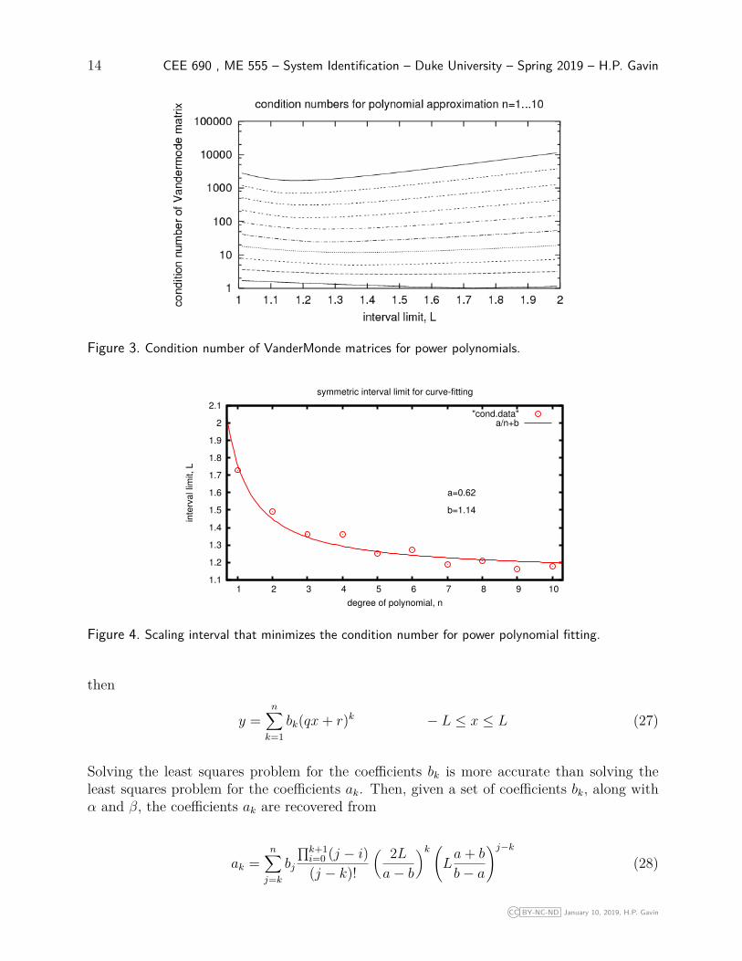
14 CEE 690 , ME 555 – System Identification – Duke University – Spring 2019 – H.P. Gavin
Figure 3. Condition number of VanderMonde matrices for power polynomials.
1.1
1.2
1.3
1.4
1.5
1.6
1.7
1.8
1.9
2
2.1
1 2 3 4 5 6 7 8 9 10
inte
rval lim
it, L
degree of polynomial, n
symmetric interval limit for curve-fitting
a=0.62
b=1.14
"cond.data"a/n+b
Figure 4. Scaling interval that minimizes the condition number for power polynomial fitting.
then
y =n∑k=1
bk(qx+ r)k − L ≤ x ≤ L (27)
Solving the least squares problem for the coefficients bk is more accurate than solving theleast squares problem for the coefficients ak. Then, given a set of coefficients bk, along withα and β, the coefficients ak are recovered from
ak =n∑j=k
bj
∏k+1i=0 (j − i)(j − k)!
( 2La− b
)k (La+ b
b− a
)j−k(28)
CC BY-NC-ND January 10, 2019, H.P. Gavin
Linear Least Squares 15
8 Orthogonal Polynomial Bases
The previous section shows that the ill-conditioned bases of high-order power polyno-mials can be partially improved by mapping the domain to [−1 : 1].
If conditioning remains a problem after mapping the domain, the power polynomialbasis can be replaced with a basis of orthogonal polynomials, for which [XTWX] is diagonalfor certain diagonal matrices W that are determined from the selected basis of orthogonalpolynomials.
A set of functions, fi(x), i = 0, · · · , n, is orthogonal with respect to some weightingfunction, w(x) in an interval α ≤ x ≤ β if
∫ β
αfi(x) w(x) fj(x) dx =
{0 i 6= jPi > 0 i = j
(29)
Furthermore, a set of functions is orthonormal if Pi = 1. Division by√Pi normalizes the set
of orthogonal functions, fi(x). For example, the sine and cosine functions are orthogonal.∫ π
−πcosmx sinnx dx = 0 ∀ m,n (30)
∫ π
−πcosmx cosnx dx =
2π m = n = 0π m = n 6= 00 m 6= n
(31)
∫ π
−πsinmx sinnx dx =
2π m = n = 0π m = n 6= 00 m 6= n
(32)
An orthogonal polynomial, fn(x) (of degree n) has n real distinct roots within the domainof orthogonality. The n roots of fn(x) are separated by the n − 1 roots of fn−1(x). Allorthogonal polynomials satisfy a recurrence relationship
Ak+1fk+1(x) = Bk+1 x fk(x) + Ck+1fk(x) +Dk+1fk−1(x), k ≥ 1 (33)
which is often useful in generating numerical values for the polynomial basis.
CC BY-NC-ND January 10, 2019, H.P. Gavin
16 CEE 690 , ME 555 – System Identification – Duke University – Spring 2019 – H.P. Gavin
8.1 Examples of Orthogonal Polynomials
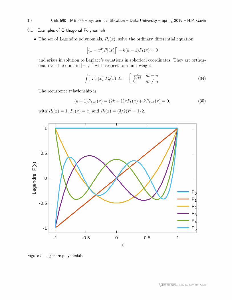
• The set of Legendre polynomials, Pk(x), solve the ordinary differential equation[(1− x2)P ′k(x)
]′+ k(k − 1)Pk(x) = 0
and arises in solution to Laplace’s equations in spherical coordinates. They are orthog-onal over the domain [−1, 1] with respect to a unit weight.
∫ 1
−1Pm(x) Pn(x) dx =
{ 22n+1 m = n
0 m 6= n(34)
The recurrence relationship is
(k + 1)Pk+1(x) = (2k + 1)xPk(x) + kPk−1(x) = 0, (35)
with P0(x) = 1, P1(x) = x, and P2(x) = (3/2)x2 − 1/2.
-1
-0.5
0
0.5
1
-1 -0.5 0 0.5 1
Lege
ndre
, P(x
)
x
P0
P1
P2
P3
P4
P5
Figure 5. Legendre polynomials
CC BY-NC-ND January 10, 2019, H.P. Gavin
Linear Least Squares 17
• Forsythe polynomials, Fk(x) are orthogonal over an arbitrary domain [α, β] with re-spect to an arbitrary weight, w(x). Weights used in curve-fitting are typically themagnitude square of the data or the inverse of the measurement error of each datapoint. The recursive generation of Forsythe polynomials is similar to Graham-Schmidtorthogonalization.
F0(x) = 1 (36)F1(x) = xF0(x)− C1F0(x) = x− C1 (37)
Applying the orthogonality condition to F0(x) and F1(x),∫ β
αF0(x) w(x) F1(x) dx = 0 (38)
leads to the condition ∫ β
αx w(x) dx = C1
∫ β
αw(x) dx. (39)
Higher degree polynomials are found by substituting the recurrence relationship
Fk+1(x) = xFk(x)− Ck+1Fk(x)−Dk+1Fk−1(x). (40)
into the orthogonality condition∫ β
αFk+1(x) w(x) Fk(x) dx = 0 (41)
and solving for Ck+1 and Dk+1 to obtain
Ck+1 =∫ βα x w(x) F 2
k (x) dx∫ βα w(x) F 2
k (x) dx(42)
Dk+1 =∫ βα x w(x) Fk(x) Fk−1 dx∫ β
α w(x) F 2k−1(x) dx
(43)
(44)
CC BY-NC-ND January 10, 2019, H.P. Gavin

18 CEE 690 , ME 555 – System Identification – Duke University – Spring 2019 – H.P. Gavin
-1
-0.5
0
0.5
1
-1 -0.5 0 0.5 1
For
syth
e, F
(x)
x
w
F0
F1
F2
F3
F4
F5
Figure 6. Forsythe polynomials on [−1, 1] orthogonal to w(x) = (0.2x2)/((x2−0.25)2 +0.2x2)
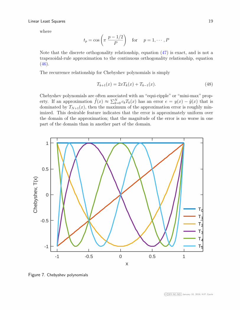
• Chebyshev polynomials Tk(x) are defined by the trigonometric expression
Tk(x) = cos(k arccosx), (45)
solve of the ordinary differential equation,
(1− x2)T ′′k (x)− xT ′k(x) + k2Tk(x) = 0 ,
and are orthogonal with respect to w(x) = (1− x2)−1/2 over the domain [−1, 1].
∫ 1
−1Tm(x) 1√
1− x2Tn(x) dx =
π m = n = 0π2 m = n 6= 00 m 6= n
(46)
The discrete form of the orthogonality condition for Chebyshev polynomials a specialdefinition because the weighting function for Chebyshev polynomials is not definedat the end-points. Given the P real roots of Tp(x), tp, p = 1, · · ·P , the discreteorthogonality relationship for Chebyshev polynomials is
P∑p=1
Tm(tp) Tn(tp) =
P m = n = 0P2 m = n 6= 00 m 6= n
(47)
CC BY-NC-ND January 10, 2019, H.P. Gavin
Linear Least Squares 19
where
tp = cos(πp− 1/2P
)for p = 1, · · · , P
Note that the discrete orthogonality relationship, equation (47) is exact, and is not atrapezoidal-rule approximation to the continuous orthogonality relationship, equation(46).
The recurrence relationship for Chebyshev polynomials is simply
Tk+1(x) = 2xTk(x) + Tk−1(x). (48)
Chebyshev polynomials are often associated with an “equi-ripple” or “mini-max” prop-erty. If an approximation f(x) ≈ ∑N
k=0 ckTk(x) has an error e = y(x) − y(x) that isdominated by TN+1(x), then the maximum of the approximation error is roughly min-imized. This desirable feature indicates that the error is approximately uniform overthe domain of the approximation; that the magnitude of the error is no worse in onepart of the domain than in another part of the domain.
-1
-0.5
0
0.5
1
-1 -0.5 0 0.5 1
Che
bysh
ev, T
(x)
x
T0
T1
T2
T3
T4
T5
Figure 7. Chebyshev polynomials
CC BY-NC-ND January 10, 2019, H.P. Gavin
20 CEE 690 , ME 555 – System Identification – Duke University – Spring 2019 – H.P. Gavin
8.2 The Application of Orthogonal Polynomials to Curve-Fitting
The benefit of curve-fitting in a basis of orthogonal polynomials is that the normalequations are diagonalized, that the model parameters may be computed directly, withoutconsideration of ill-conditioned systems of equations or numerical linear algebra, and thatthe parameter errors are uncorrelated.
The cost of curve-fitting in a basis of orthogonal polynomials is that the basis mustbe constructed in a way that preserves the discrete orthogonality conditions. For Legendrepolynomials the values of the independent variables must be uniformly spaced and mappedto the interval [−1 : 1], For Chebyshev polynomials the values of the independent variablesmust be the roots of a high-order Chebyshev polynomial. In both of these bases the datay must be interpolated to the specified values of the independent variables. For a Forsythebasis, the data need not be mapped or interpolated.
Consider Chebyshev approximation in which the mapping and interpolation steps havealready been carried out.
ep = yp − y(tp; c) = yp −n∑k=0
ckTk(tp) (49)
which may be written for all m data points,
e1e2...em
=
y1y2...ym
−
1 T1(t1) T2(t1) · · · Tn(t1)1 T1(t2) T2(t2) · · · Tn(t2)... ... ... . . . ...1 T1(tm) T2(tm) · · · Tn(tm)
c0c1c2...cn
, (50)
or e = y − Tc. Values tp are roots of a high order Chebyshev polynomial and data points yphave been interpolated to points tp.
Minimizing the quadratic objective function J = ∑e2p leads to the normal equations
c = [TTT ]−1TTy, (51)
where [TTT ] is diagonal as per the discrete orthogonality relation, equation (47)
[TTT ] =
∑T1(tp)T1(tp)
∑T1(tp)T2(tp)
∑T1(tp)T3(tp) · · ·
∑T1(tp)Tn(tp)∑
T2(tp)T2(tp)∑T2(tp)T3(tp) · · ·
∑T2(tp)Tn(tp)∑
T3(tp)T3(tp) · · ·∑T3(tp)Tn(tp)
sym . . . ...∑Tn(tp)Tn(tp)
=
P 0 0 · · · 00 P/2 0 · · · 00 0 P/2 · · · 0... ... ... . . . ...0 0 0 · · · P/2
(52)
CC BY-NC-ND January 10, 2019, H.P. Gavin
Linear Least Squares 21
The discrete orthogonality of Chebyshev polynomials is exact to within machine precision,regardless of the number of terms in the summation. Because [TTT ] may be inverted ana-lytically, the curve-fit coefficients may be computed directly from
c0 = 1P
P∑p=1
y(tp) (53)
ck = 2P
P∑p=1
Tk(tp)y(tp), for k > 0 (54)
Also, note that Tk(tp) = cos(kπ(p − 1/2)/P ). The cost of the simplicity of the closed-formexpression for ck using the Chebyshev polynomial basis is the need to re-scale the independentvariables, x to the interval [−1, 1], and to interpolate the data, y, to the roots of TP (x).
Coefficients estimated in an orthogonal polynomial basis have a diagonal covariancematrix, as per equations (52) and (16); parameter errors are uncorrelated.
CC BY-NC-ND January 10, 2019, H.P. Gavin
22 CEE 690 , ME 555 – System Identification – Duke University – Spring 2019 – H.P. Gavin
9 Tikhonov Regularization
The goal of regularization is to modify the normal equations [XTX]a = XTy in order tosignificantly improve its condition number while leaving the solution a relatively un-changed.
In Tikhonov regularization the least-squares error criterion is augmented with a quadraticterm involving the parameters. The effect of Tikhonov regularization is to estimate modelparameters while also keeping the model parameters near zero, or near some other set ofvalues. Doing so improves the conditioning of the normal equations.
Consider the over-determined system of linear equations y = Xa where y ∈ Rm anda ∈ Rn, and m > n. We seek the solution a that minimizes the quadratic objective function
J(a) = ||Xa− y||2P + β||a− a||2Q, (55)
where the quadratic vector norm is defined as ||x||2P = xTPx, in which the weighting matrixP is positive definite, and the Tikhonov regularization factor β is non-negative. If the vectory is obtained through imprecise measurements, and the measurements of each element of yiare statistically independent, then P is typically a diagonal matrix in which each diagonalelement Pii is the inverse of the variance of the measurement error of yi, Pii = 1/σ2
yi. If the
errors in yi are not statistically independent, then P should be the inverse of the covariancematrix Vy of the vector y, P = V−1
y . The positive definite matrix Q and the referenceparameter vector a reflect the way in which we would like to constrain the parameters. Forexample, we may simply want the solution, a to be near some reference point, a, in whichcase Q = In. Alternatively, we may wish some linear function of the parameters LQa to beminimized, in which case Q = LT
QLQ and a = 0. Expanding the quadratic objective function,
J(a) = aTXTPXa− 2aTXTPy + yTPy + βaTQa− 2βaTQa+ βaTQa. (56)
The objective function is minimized by setting the first partial of J(a) with respect to a equalto zero,
∂J(a)∂a
T
= 2XTPXa− 2XTPy + 2βQa− 2βQa = 0n×1, (57)
and solving for the parameter estimates a,
a(β) = [XTPX + βQ]−1(XTPy + βQa). (58)
The meaning of the notation a(β) is that the solution a depends upon the value of theregularization factor, β. The regularization factor weights the relative importance of ||Xa−y||2P and ||a − a||2Q. For problems in which X or XTPX are ill-conditioned, small values ofβ (i.e., small compared to the average of the diagonal elements of XTPX) can significantlyimprove the conditioning of the problem.
If the measurement errors of yi are not individually known, then it is common to setP = In. Likewise, if the n parameter differences a − a are all equally important, then itis customary to set Q = In. Finally, if we have no set of reference parameters a, thenit is common to set a = 0. With these simplifications, the solution is given by a(β) =
CC BY-NC-ND January 10, 2019, H.P. Gavin
Linear Least Squares 23
[XTX + βIn]−1XTy, which may be written a(β) = X+(β)y, where X+
(β) is called the regularizedpseudo-inverse. In the more general case, in which P 6= In and Q 6= In, but a = 0n×1,
X+(β) = [XTPX + βQ]−1XTP. (59)
The dimension of X+(β) is n ×m. In a later section we will see that if LQ is inevitable then
we can always scale and shift X, y, and a with no loss of generality.
9.1 Error Analysis of Tikhonov Regularization
We are interested in determining the covariance matrix of the solution a(β).
Va(β) =[∂a(β)
∂y
]Vy
[∂a(β)
∂y
]T
= X+(β) VyX
+T(β)
= [XTPX + βQ]−1XTP Vy PX[XTPX + βQ]−1
= [XTPX + βQ]−1XTPX[XTPX + βQ]−1, (60)
where we use P = V−1y . This covariance matrix is sometimes called the error propagation
matrix, as it indicates how random errors in y propagate to the estimates a. Note that inthe special case of no regularization (β = 0),
Va(0) = [XTPX]−1, (61)
and that the parameter covariance matrix with regularization is always smaller than thatwithout regularization.
In addition to having propagation errors, the estimate a(β) is biased by the regularizationfactor. Let us presume that we know y exactly, and that the exact value of y is ye. Theexact solution, without regularization, is ae = [XTPX]−1XTPye. The regularization error,δa(β) = a(β) − ae (for a = 0), is
δa(β) = [X+(β) −X
+(0)]ye
= [[XTPX + βQ]−1XTP − [XTPX]−1XTP ]ye
= [[XTPX + βQ]−1 − [XTPX]−1]XTPye. (62)
Recall that ae = [XTPX]−1XTPye, or XTPXae = XTPye, so
δa(β) = [[XTPX + βQ]−1 − [XTPX]−1]XTPXae
= [[XTPX + βQ]−1XTPX − In]ae
= [XTPX + βQ]−1[XTPX + βQ− βQ]ae − Inae
= [XTPX + βQ]−1[XTPX + βQ]ae − [XTPX + βQ]−1βQae − Inae
= −[XTPX + βQ]−1Qβae. (63)
The regularization error δa(β) equals zero if β = 0 and increases with β.
The total mean squared error matrix, E(β) is the sum of the parameter covariancematrix and the regularization bias error, E(β) = Va(β) +δa(β)δa
T(β). The mean squared error
is the trace of E(β).
CC BY-NC-ND January 10, 2019, H.P. Gavin
24 CEE 690 , ME 555 – System Identification – Duke University – Spring 2019 – H.P. Gavin
10 Singular Value DecompositionConsider a real matrix X that is not necessarily square, X ∈ Rm×n, with m > n. The
rank of X is r and r ≤ n. Let λ1, λ2, · · · , λr be the positive eigenvalues of [XTX], includingmultiplicity, ordered in decreasing numerical order, λ1 ≥ λ2 ≥ · · · ≥ λr > 0. The singularvalues, σi of X are defined as the square roots of the eigenvalues, σi =
√λi, i = 1, · · · , r.
The singular value decomposition of a matrix X (X ∈ Rm×n, m ≥ n) is given by thefactorization
X = UΣV T (64)where U ∈ Rm×m, Σ ∈ Rm×n and V ∈ Rn×n. The matrices U and V are orthonormal,UTU = Im and V TV = In, and Σ is a diagonal matrix of the singular values of X, Σ =diag(σ1 σ2 · · · σn). The singular values of X are sorted in a non-increasing numerical order,σ1 ≥ σ2 ≥ · · · ≥ σn ≥ 0. The number of singular values equal to zero is equal to thenumber of linearly dependent columns of X. If r is the rank of X then n− r singular valuesare equal to zero. The ratio of the maximum to the minimum singular value is called thecondition number of X, cX = σ1/σn. Matrices with very large condition numbers are said tobe ill-conditioned. If σn = 0, then cX =∞ and X is said to be singular, and is non-invertible.
The columns of U and V are called the right and left singular vectors, U = [u1 u2 · · · um]and V = [v1 v2 · · · vn]. The left singular vectors ui are column vectors of dimension m andthe right singular vectors vi are column vectors of dimension n. If one or more singular valueof X is equal to zero, r < n, and the set of right singular vectors {vr+1 · · · vn} (correspondingto σr+1 = · · · = σn = 0) form an orthonormal basis for the null-space of X. The dimensionof the null space of X plus the rank of X equals n.
The singular value decomposition of X may be written as an expansion of the singularvectors,
X =n∑i=1
σi[uivTi ], (65)
where the rank-1 matrices [uivTi ] have the same dimension as X. Also note that ||ui||I =
||vi||I = 1. Therefore, the significance of each term of the expansion σiuivTi decreases with i.
The system of equations y = Xa may be inverted using singular value decomposition:a = V Σ−1UTy, or
a =n∑i=1
1σiviu
Ti y. (66)
The singular values in the expansion which contribute least to the decomposition of X canpotentially dominate the solution a. An additive perturbation δy in y will propagate to aperturbation in the solution, δa = V Σ−1UTδy. The magnitude of δa in the direction of vi isequal to the dot product of ui with δy divided by σi,
vTi δa = 1
σiuTi δy. (67)
Therefore, perturbations δy that are orthogonal to all of the left singular vectors, ui, are notpropagated to the solution. Conversely, any perturbation δa in the direction of vi contributesto y in the direction of ui by an amount equal to σi||δa||.
CC BY-NC-ND January 10, 2019, H.P. Gavin
Linear Least Squares 25
If the rank of X is less than n, (r < n), the components of a which lie in the spacespanned by {vr+1 · · · vn} will have no contribution to y. In principle, this means that anycomponent of y in the space spanned by the sub-set of left singular vectors {ur+1 · · · um}is an “error” or is “noise”, since it can not be obtained using the expression y = Xa forany value of a. These components of y are called “noise” or “error” because they can notbe predicted by the model equations, y = Xa. In addition, these “noisy” components of y,which lie in the space {ur+1 · · · um}, will be magnified to an infinite degree when used toidentify the model parameters a.
From the singular value decomposition of X we find that XTX = V Σ2V T. If c isthe condition number of X, then the condition number of XTX is c2. If c is large, solving[XTX]a = XTy can be numerically treacherous.
When X is obtained using measured data, it is almost never singular but is often ill-conditioned. We will consider two types of ill-conditioned matrices: (i) matrices in which thefirst r singular values are all much larger than the last n−r singular values, and (ii) matricesin which the singular values decrease at a rate that is more or less uniform.
10.1 Truncated Singular Value Expansion
If the first r singular values are much larger than the last n−r singular values, (i.e., σ1 ≥σ2 ≥ · · · ≥ σr >> σr+1 ≥ σr+2 ≥ · · · ≥ σn ≥ 0), then a relatively accurate representation ofX may be obtained by simply retaining the first r singular values of X and the correspondingcolumns of U and V ,
X(r) = UrΣrVTr =
r∑i=1
σiuivTi , (68)
and the truncated expression for the parameter estimates is
a(r) = VrΣ−1r V T
r y =r∑i=1
1σiviu
Ti y , (69)
where Vr and Ur contain the first r rows of V and U , and where Σr contains the first r rowsand columns of Σ.
If σr+1 is close to the numerical precision of the computation, ε (ε ≈ 10−6 for singleprecision and ε ≈ 10−12 for double precision), then the singular values, σr+1 · · · σn and thecorresponding columns of U and V contribute negligibly to X. Their contribution to thesolution vector, a, can be dominated by random noise and round-off error in y.
The parameter estimate covariance matrix is derived using equation (4), in which[∂a
∂y
]= VrΣ−1
r UTr , (70)
Therefore the covariance matrix of the parameter estimates is
Va(r) = VrΣ−1r UT
r Vy UrΣ−1r V T
r . (71)
CC BY-NC-ND January 10, 2019, H.P. Gavin
26 CEE 690 , ME 555 – System Identification – Duke University – Spring 2019 – H.P. Gavin
Because the solution a(r) does not contain components that are close to the null-space ofX the covariance matrix is limited to the range of X for which the singular values are notunacceptably large. The cost of the reduced parameter covariance matrix is an increased biaserror, introduced through truncation. Assuming that we know y exactly, the correspondingexact solution with no regularization ae can be used to evaluate regularization bias error,δa(r) = a(r) − ae.
δa(r) = VrΣ−1r UT
r ye − V Σ−1UTye (72)
Substituting V ΣUT = UrΣrVTr + UnΣnV
Tn ,
δa(r) = −[VnΣ−1n UT
n ]ye, (73)
where Vn and Un contain the last n − r rows of V and U , and where Σn contains the lastn− r rows and columns of Σ. Substituting ye = UΣV Tae,
δa(r) = −[VnΣ−1n UT
n UΣV T]ae (74)
Noting that UTn U = Σ−1
n UTn UΣ = [0n−r×r In−r],
δa(r) = −[VnV Tn ]ae (75)
Note that while the matrix −V Tn Vn equals In−r, the matrix −VnV T
n is not identity becausethe summation is only over the last n− r rows of V .
The total mean squared error matrix, E(r) is the sum of the parameter covariance matrixand the truncation bias error, E(r) = VrΣ−1
r UTr Vy UrΣ−1
r V Tr − VnV T
n ae. The mean squarederror is the trace of E(r).
10.2 Singular Value Decomposition with Tikhonov Regularization
If the singular values decrease at a rate that is more or less uniform, then selecting rfor the truncated approximations above may require some subjective reasoning. Certainlyany singular value that is equal to or less than the precision of the computation should beeliminated. However, if σ1 ≈ 1015 and σn ≈ 10−3, X would be considered ill conditioned bymost standards, even though the smallest singular value can be resolved even with single-precision computations. As an alternative to eliminating one or more of the smallest singularvalues one may simply add a small constant β to all of the singular values. This can substan-tially improve the condition number of the system without eliminating any of the informationcontained in the full singular value factorization. This approach is equivalent to Tikhonovregularization.
To link the formulation of Tikhonov regularization to singular value decomposition, itis useful to show that a the Tikhonov objective function (55) may be written
J(a) = ||Xa− y||2I + β||a||2I + C, (76)
by simply scaling and shifting X, y, and a, and with no loss of generality. In the aboveexpression, C is independent of a and does not affect the parameter estimates. Defining LP
CC BY-NC-ND January 10, 2019, H.P. Gavin
Linear Least Squares 27
and LQ as the Cholesky factors of P and Q, and defining X = LPXL−1Q , y = LP (y −Xa),
and a = LQ(a− a) then equation (55) is equivalent to equation (76), where
C = aTXTLTPLPXa− 2aTXTLT
PLPy (77)
Setting [∂J(a)/∂a]T to zero results in the least-squares parameter estimates
ˆa(β) = [XTX + βI]−1XTy. (78)
Note that the solutions a(β) and ˆa(β) are related by the scaling
a(β) = L−1Q
ˆa(β) + a. (79)
In other words, the minimum value of the objective function (55) coincides with the minimumvalue of the objective function (76). As a simple example of the effects of scaling on theparameter estimates, consider the two equivalent quadratic objective functions J(a) = 5a2−3a+1 and J(a) = 20a2−6a+2, where a is scaled, a = 2a. The parameter estimates a = 3/10and˜a = 3/20. These estimates satisfy the scaling relationship, a = 2ˆa.
The singular value decomposition of X may be substituted into the least-squares solu-tion for ˆa(β)
ˆa(β) = [V ΣUTUΣV T + βI]−1V ΣUTy
= [V Σ2V T + βV IV T]−1V ΣUTy
= [V (Σ2 + βI)V T]−1V ΣUTy
= V (Σ2 + βI)−1V TV ΣUTy
= V (Σ2 + βI)−1ΣUTy (80)
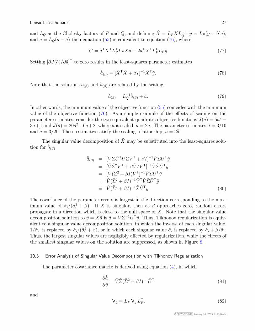
The covariance of the parameter errors is largest in the direction corresponding to the max-imum value of σi/(σ2
i + β). If X is singular, then as β approaches zero, random errorspropagate in a direction which is close to the null space of X. Note that the singular valuedecomposition solution to y = Xa is a = V Σ−1UTy. Thus, Tikhonov regularization is equiv-alent to a singular value decomposition solution, in which the inverse of each singular value,1/σi, is replaced by σi/(σ2
i + β), or in which each singular value σi is replaced by σi + β/σi.Thus, the largest singular values are negligibly affected by regularization, while the effects ofthe smallest singular values on the solution are suppressed, as shown in Figure 8.
10.3 Error Analysis of Singular Value Decomposition with Tikhonov Regularization
The parameter covariance matrix is derived using equation (4), in which
∂ˆa∂y
= V Σ(Σ2 + βI)−1UT (81)
andVy = LP Vy L
TP . (82)
CC BY-NC-ND January 10, 2019, H.P. Gavin
28 CEE 690 , ME 555 – System Identification – Duke University – Spring 2019 – H.P. Gavin
1
10
100
0.01 0.1 1
σi /
( σ
i2+
β )
σi
β=0
β=0.0001
β=0.001
β=0.01
β=0.1
Figure 8. Effect of regularization on singular values.
Recall that Vy is the covariance matrix of the measurement errors, and that P = V−1y = LT
PLP .Using the fact that (AB)−1 = B−1A−1, we find that Vy = I. Therefore the covariance matrixof the solution is
Vˆa(β) = V Σ2(Σ2 + βI)−2V T. (83)Because [∂a/∂a] = L−1
Q , the covariance matrix of the original solution is
Va(β) = L−1Q V Σ2(Σ2 + βI)−2V TL−TQ . (84)
As in equation (60), we see here that increasing β reduces the covariance of the propagatederror quadratically. The cost of the reduced parameter covariance matrix is a bias error,introduced through regularization. Assuming that we know y exactly, the correspondingexact solution with no regularization ae can be used to evaluate regularization bias error,δa(β) = ˆa(β) − ae.
δa(β) = V Σ(Σ2 + βI)−1UTye − V Σ−1UTye
= [V Σ(Σ2 + βI)−1UT − V Σ−1UT]ye (85)
Substituting ye = UΣV Tae, and UTU = I
δa(β) = [V (Σ2 + βI)−1Σ2V T − I]ae
= [V (Σ2 + βI)−1(Σ2 + βI − βI)V T − I]ae
= −V (Σ2 + βI)−1βV Tae (86)
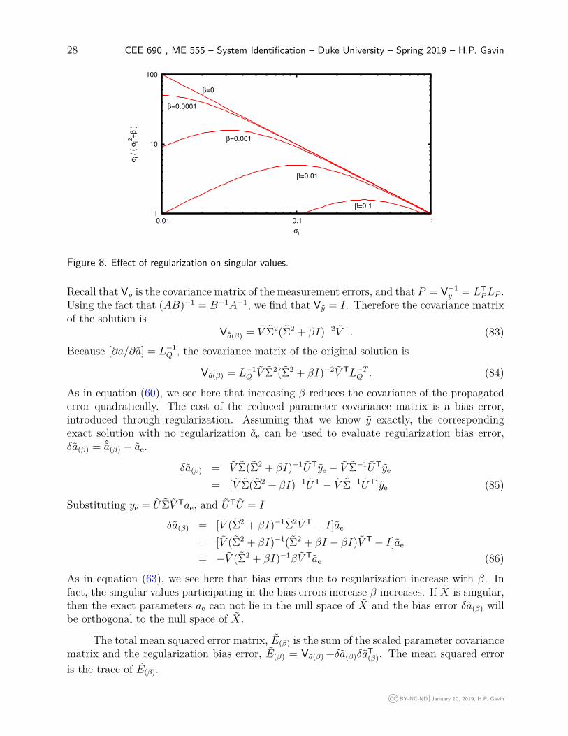
As in equation (63), we see here that bias errors due to regularization increase with β. Infact, the singular values participating in the bias errors increase β increases. If X is singular,then the exact parameters ae can not lie in the null space of X and the bias error δa(β) willbe orthogonal to the null space of X.
The total mean squared error matrix, E(β) is the sum of the scaled parameter covariancematrix and the regularization bias error, E(β) = Va(β) +δa(β)δa
T(β). The mean squared error
is the trace of E(β).
CC BY-NC-ND January 10, 2019, H.P. Gavin
Linear Least Squares 29
0.1
1
0.01 0.1 1
β / (
σi2
+β )
σi
β=0.0001 β=0.001 β=0.01 β=0.1
Figure 9. Effect of regularization on bias errors.
10.4 Scaling of Units and Singular Value Decomposition
In most instances, elements of y and a have dissimilar units. In such cases the condi-tioning of X is affected by the system of units used to describe the elements of y and a (andX). The measurements y and the parameters a may be scaled using diagonal matrices Dy
and Da, y = Dyy, a = Daa. Since Dyy = XDaa, y = D−1y XDaa, and the system matrix for
the scaled system is X = D−1y XDa. Defining SVD’s: X = UΣV T and X = UΣV T, the effect
of scaling on the singular values is apparent Σ = UTD−1y UΣV TDaV .
Parameter scaling matrices can be designed to achieve a desired spectrum of singularvalues. But this appears to be a nonlinear problem requiring an iterative method to updateDa and Dy such that the condition number of D−1
y XDa converges to a minimum value, whilepossibly meeting other constraints, such as bounds on the values of Da and Dy.
CC BY-NC-ND January 10, 2019, H.P. Gavin
30 CEE 690 , ME 555 – System Identification – Duke University – Spring 2019 – H.P. Gavin
11 Numerical Example
Consider the singular system of equations yo = Xo a,[1001000
]=[
1 1010 100
] [a1a2
](87)
The singular value decomposition of Xo is
U =[−0.0995037 −0.995037−0.995037 0.0995037
]
Σ =[
101 00 0
]
V =[−0.0995037 0.995037−0.995037 −0.0995037
]
Even though Xo is a singular matrix, the estimates for this particular system is defined. Thesecond column of V gives the one-dimensional null-space of Xo. Note that yo in equation (87)is normal to u2. Vectors yo normal to the space spanned by Un are “noise-free” in the sensethat no components of yo propagates to the null space of Xo. The singular value expansionfor the estimates gives[
a1a2
]= 1
101
[−0.0995037−0.995037
] [−0.0995037 −0.995037
] [ 1001000
]+
10
[0.995037
−0.0995037
] [−0.995037 0.0995037
] [ 1001000
]+
=[
0.990099009.9009900
](88)
The zero singular value does not affect the estimates because y is orthogonal to u2. It isinteresting to note that despite the fact that the two equations in equation (87) representthe same line (infinitely many solutions) the SVD provides a unique solution, (provided that0/0 is evaluated to 0).
Regularization works very well for problems in which UTn y is very small. Applying
regularization to this problem we seek estimates a that minimizes the quadratic objectivefunction of equation (55). In other words, we want to find the solution to y = Xoa, whilekeeping the estimates, a close to a. How much we care that a is close to a is determined bythe regularization parameter, β. In general β should be some small fraction of the averageof the diagonal elements of X, β << trace(X)/n. Increasing β will make the problem easierto solve numerically, but will also add bias to the estimates. The philosophy of using theregularization parameter is something like this: Let’s say we have a problem which we can’tsolve, (i.e., det(X) = 0 ). Regularization slightly changes the problem into a problem thatdoes have a solution which is ideally independent of the amount of the perturbation.
CC BY-NC-ND January 10, 2019, H.P. Gavin
Linear Least Squares 31
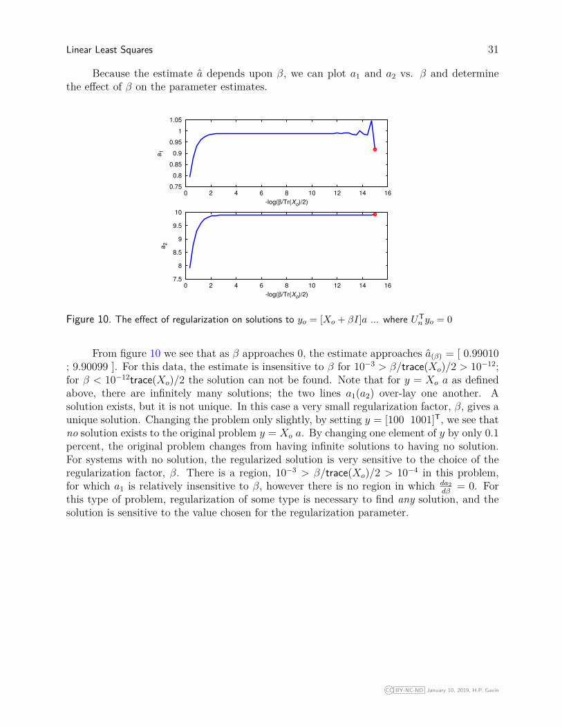
Because the estimate a depends upon β, we can plot a1 and a2 vs. β and determinethe effect of β on the parameter estimates.
7.5
8
8.5
9
9.5
10
0 2 4 6 8 10 12 14 16
a2
-log(β/Tr(Xo)/2)
0.75
0.8
0.85
0.9
0.95
1
1.05
0 2 4 6 8 10 12 14 16
a1
-log(β/Tr(Xo)/2)
Figure 10. The effect of regularization on solutions to yo = [Xo + βI]a ... where UTn yo = 0
From figure 10 we see that as β approaches 0, the estimate approaches a(β) = [ 0.99010; 9.90099 ]. For this data, the estimate is insensitive to β for 10−3 > β/trace(Xo)/2 > 10−12;for β < 10−12trace(Xo)/2 the solution can not be found. Note that for y = Xo a as definedabove, there are infinitely many solutions; the two lines a1(a2) over-lay one another. Asolution exists, but it is not unique. In this case a very small regularization factor, β, gives aunique solution. Changing the problem only slightly, by setting y = [100 1001]T, we see thatno solution exists to the original problem y = Xo a. By changing one element of y by only 0.1percent, the original problem changes from having infinite solutions to having no solution.For systems with no solution, the regularized solution is very sensitive to the choice of theregularization factor, β. There is a region, 10−3 > β/trace(Xo)/2 > 10−4 in this problem,for which a1 is relatively insensitive to β, however there is no region in which da2
dβ= 0. For
this type of problem, regularization of some type is necessary to find any solution, and thesolution is sensitive to the value chosen for the regularization parameter.
CC BY-NC-ND January 10, 2019, H.P. Gavin
32 CEE 690 , ME 555 – System Identification – Duke University – Spring 2019 – H.P. Gavin
7
7.5
8
8.5
9
9.5
10
10.5
11
0 0.5 1 1.5 2 2.5 3 3.5 4
a2
-log(β/Tr(Xo)/2)
-6
-5
-4
-3
-2
-1
0
1
0 0.5 1 1.5 2 2.5 3 3.5 4
a1
-log(β/Tr(Xo)/2)
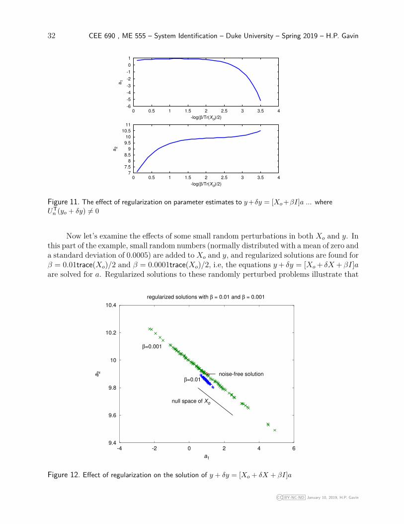
Figure 11. The effect of regularization on parameter estimates to y+δy = [Xo+βI]a ... whereUTn (yo + δy) 6= 0
Now let’s examine the effects of some small random perturbations in both Xo and y. Inthis part of the example, small random numbers (normally distributed with a mean of zero anda standard deviation of 0.0005) are added to Xo and y, and regularized solutions are found forβ = 0.01trace(Xo)/2 and β = 0.0001trace(Xo)/2, i.e, the equations y+ δy = [Xo + δX +βI]aare solved for a. Regularized solutions to these randomly perturbed problems illustrate that
9.4
9.6
9.8
10
10.2
10.4
-4 -2 0 2 4 6
a2
a1
regularized solutions with β = 0.01 and β = 0.001
noise-free solution
null space of Xo
β=0.001
β=0.01
Figure 12. Effect of regularization on the solution of y + δy = [Xo + δX + βI]a
CC BY-NC-ND January 10, 2019, H.P. Gavin

Linear Least Squares 33
at a regularization factor, β ≈ 0.01trace(Xo)/2, the solution is relatively insensitive to thevalue of β. Comparing the solutions for 100 randomly perturbed problems, we find thatthe variance among the solutions is less than 1. For a regularization factor of 0.001, onthe other hand, we see that the variance of the solution is quite a bit larger, but that themean value of all of the solutions is much closer to the noise-free solution. This illustratesthe fact that larger values of β decrease the propagation error but introduce a bias error.If no regularization is used, then a1 and a2 range from -1000 to +1000 and from -100 to100, respectively, in this Monte Carlo analysis. Adding the small levels of noise to the non-invertible matrix Xo makes it invertible, however, the solution depends largely on the noiselevel. In fact if no regularization is used, the solution to this problem depends almost entirelyon the noise in the matrices. Increasing the regularization factor, β, reduces the propagationof random noise in the solution at the cost of a bias error.
12 Constrained Least Squares
Suppose that in addition to minimizing the sum-of-squares-of-errors, the curve-fit mustalso satisfy other criteria. For example, suppose that the curve-fit must pass through aparticular point (xc, yc), or that the slope of the curve at a particular location, xs, must beexactly a given value, y′s. Equality constraints such as these are linear in the parametersand are a natural application of the method of Lagrange multipliers. In general, equalityconstraints that are linear in the parameter may be expressed as Ca = b. The constrainedleast-squares problem is to minimize χ2(a) such that Ca = b. The augmented objectivefunction (the Lagrangian) becomes,
χ2A(a, λ) = aTXT V−1
y Xa− aTXT V−1y y − yT V−1
y Xa+ yT V−1y y + λT(Ca− b) (89)
Minimizing χ2A with respect to a and maximizing χ2
A with respect to λ results in a system oflinear equations for the coefficient estimates a and Lagrange multipliers λ.[
2XT V−1y X CT
C 0
] [a
λ
]=[
2XT V−1y y
b
](90)
If the curve-fit problem has n coefficients and c constraint equations, then the matrix issquare and of size (n+ c)× (n+ c).
CC BY-NC-ND January 10, 2019, H.P. Gavin
34 CEE 690 , ME 555 – System Identification – Duke University – Spring 2019 – H.P. Gavin
13 Recursive Least Squares
When data points are provided sequentially, parameter estimates a(m) can be updatedwith each new observation, (xm+1, ym+1).
Given a set of m measurement points and estimates of model parameters a(m) corre-sponding to the data set (xi, yi), i = 1, ...,m, we seek an update to the model parametersa(m+1) from a new measurement xm+1, ym+1.
Presuming a linear model, y(x; a) = Xa, we define the i-th rows of X as xi so thaty1...ym
=
− x1 −
...− xm −
a1...an
The least-squares error criterion is
J(m) =m∑i=1||yi − yi||2F
=m∑i=1
(yi − xia)T(yi − xia)
=m∑i=1
(yTi yi − 2yT
i xia+ aTxTi xia)
and applying the necessary condition for optimality,(∂J(m)
∂a
)T
= 0 :m∑i=1
[xTi xi]a(m) =
m∑i=1
xTi yi
Defining some new terms to simplify the notation,
R(m) =m∑i=1
[xTi xi]
andq(m) =
m∑i=1
xTi yi ,
we see that R(m) is a sum of rank-1 matrices. and it can be viewed as an auto-correlation ofthe sequence of the rows xi of the model basis X, in the special case that xi have a mean ofzero. The matrix R−1
(m) is interpreted as the parameter estimate covariance matrix, [XTX]−1.The (column) vector q(m) can be viewed as a cross-correlation between the rows of the modelbasis and the data, in the special case that xi and yi have a mean of zero. Given a newmeasurement (xm+1, ym+1),
R(m+1) = R(m) + xTm+1xm+1
andq(m+1) = q(m) + xT
m+1ym+1
CC BY-NC-ND January 10, 2019, H.P. Gavin
Linear Least Squares 35
and the model parameters incorporating information from the new data points satisfy
R(m+1)a(m+1) = q(m+1) (91)
With a known value of a matrix inverse, R−1, the inverse of R + xTx can be computed viathe Sherman-Morrison Update identity
(R + xTx)−1 = R−1 −R−1xT(1 + xR−1xT
)−1xR−1 (92)
Defining more notation to simplify expressions,
K(m+1) = R−1(m) −R
−1(m)x
Tm+1(1 + xm+1R
−1(m)x
Tm+1)−1
the rank-1 update of the updated parameter covariance becomes
R−1(m+1) = R−1
(m) −K(m+1)xm+1R−1(m) (93)
With this we can write K(m+1) as
K(m+1) = R−1(m+1)x
Tm+1 (94)
= R−1(m)x
Tm+1
(1 + xm+1R
−1(m)x
Tm+1
)−1
which can be shown as follows
K(m+1)(1 + xm+1R
−1(m)x
Tm+1
)= R−1
(m)xTm+1
K(m+1) +K(m+1)xm+1R−1(m)x
Tm+1 = R−1
(m)xTm+1
K(m+1) = R−1(m)x
Tm+1 −K(m+1)xm+1R
−1(m)x
Tm+1
=(R−1
(m) −K(m+1)xm+1R−1(m)
)xTm+1
= R−1(m+1)x
Tm+1
Now, introducing a model prediction
ym+1 = xm+1a(m) = xm+1R−1(m)q(m) (95)
and combining equations (91) to (95), the update of the model parameter estimates can bewritten,
a(m+1) = a(m) +K(m+1) (ym+1 − ym+1) (96)The role of K(m+1) can be interpreted as an update gain which provides the sensitivity ofthe model parameter update to differences between the measurement ym+1 and its predictedvalue ym+1. This prediction error is called an innovation. The model parameter updateidentity can be shown as follows:
a(m+1) = R−1(m+1)q(m+1)
=(R−1
(m) −K(m+1)xm+1R−1(m)
) (q(m) + xm+1ym+1
)= R−1
(m)q(m) −K(m+1)xm+1R−1(m)q(m) +R−1
(m)xm+1ym+1 −K(m+1)xm+1R−1(m)xm+1ym+1
= a(m) −K(m+1)ym+1 +(R−1
(m) −K(m+1)xm+1R−1(m)
)xm+1ym+1
= a(m) −K(m+1)ym+1 +R−1(m+1)xm+1ym+1
= a(m) +K(m+1) (ym+1 − ym+1)
CC BY-NC-ND January 10, 2019, H.P. Gavin
36 CEE 690 , ME 555 – System Identification – Duke University – Spring 2019 – H.P. Gavin
In many applications of recursive-least squares it is desirable for the most-recent data to havea larger effect upon the parameter estimates. In these situations, the least-squares objectivecan be exponentially weighted
J(m) =m∑i=1
λm−i||yi − yi||2 0� λ < 1
Typical values for the exponential forgetting factor λ are close to 1 (e.g., 0.98 to 0.995).Carrying λ through the previous development (91) to (96) we arrive at the recursive leastsquares procedure
1. initialize variables ... m = 0, R−1(m) = δIn where δ ≥ 100σ2
x or R−1(m) =
[0∑
i=−lλ−ixT
i xi
]−1
,
and a(m) = 0 or a knowledgeable guess,
2. collect xm+1
3. compute the update gain ... K(m+1) = R−1(m)x
Tm+1
(λ+ xm+1R
−1(m)x
Tm+1
)−1
4. predict the next measurement ... ym+1 = xm+1a(m)
5. collect ym+1
6. update the model parameters ... a(m+1) = a(m) +K(m+1) (ym+1 − ym+1)
7. update the parameter covariance ... R−1(m+1) =
(R−1
(m) −K(m+1)xm+1R−1(m)
)/λ
8. increment m ... m = m+ 1 and go to step 2.
Notes:
• If the update gain is very small, the model parameter update is not sensitive to largeprediction errors.
• The update gain decreases monotonically; λ keeps the update gain from becoming toosmall too fast.
• The update gain increases with larger values of the parameter covariance R−1.
• The update gain can be interpreted as K ∼ Va/(1 + Vy). A large parameter covarianceimplies large uncertainty in the parameters, and the need for a parameter update thatis sensitive to prediction errors (large K). A large model prediction covariance impliesnoisy data, and the need for a parameter update that is insensitive to prediction errors(small K).
• Likewise, smaller values of λ keep the parameter covariance matrix R−1(m+1) from getting
too small too fast.
• With λ = 1 the RLS estimates a(m) equals the OLS estimates [XTX]−1XTy obtainedfrom m data points.
CC BY-NC-ND January 10, 2019, H.P. Gavin

Linear Least Squares 37
13.1 The Sherman-Morrison rank-1 update identity
The Sherman-Morrison Update identity provides the inverse of (R + xTx) in terms ofx and the inverse of R. Defining,
R(m+1) = R(m) + xTx
we have (R(m) + xTx
)R−1
(m+1) = I
which is equivalent to [R(m) xT
x −1
] [R−1
(m+1)z
]=[I0
]To show this, we break the above matrix equation into two separate matrix equations,
R(m)R−1(m+1) + xTz = I (97)xR−1
(m+1) − z = 0 (98)
and substitute the second equation into the first,
R(m)R−1(m+1) + xTxR−1
(m+1) = I
which shows that (R(m) + xTx
)R−1
(m+1) = I .
Now re-arraging the first equation,
R−1(m+1) = R−1
(m)(I − xTz) (99)
and substituting equation (99) into (98) we solve for z,
z = xR−1(m)(I − x
Tz)= xR−1
(m) − xR−1(m)x
Tz(1 + xR−1
(m)xT)z = xR−1
(m)
z =(1 + xR−1
(m)xT)−1
xR−1(m) (100)
Finally, inserting (100) into (99) we have the Sherman-Morrison Update identity.
R−1(m+1) = R−1
(m)
(I − xT
(1 + xR−1
(m)xT)−1
xR−1(m)
)R−1
(m+1) = R−1(m) −R
−1(m)x
T(1 + xR−1
(m)xT)−1
xR−1(m)
CC BY-NC-ND January 10, 2019, H.P. Gavin
38 CEE 690 , ME 555 – System Identification – Duke University – Spring 2019 – H.P. Gavin
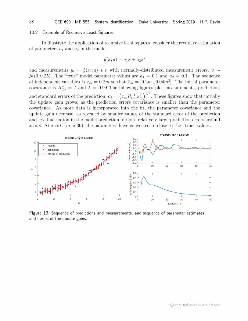
13.2 Example of Recursive Least Squares
To illustrate the application of recursive least squares, consider the recursive estimationof parameters a1 and a2 in the model
y(x; a) = a1x+ a2x2
and measurements yi = y(xi; a) + v with normally-distributed measurement errors, v ∼N (0, 0.25). The “true” model parameter values are a1 = 0.1 and a2 = 0.1. The sequenceof independent variables is xm = 0.2m so that xm = [0.2m , 0.04m2]. The initial parametercovariance is R−1
(0) = I and λ = 0.99 The following figures plot measurements, prediction,
and standard errors of the prediction, σy =(xmR
−1(m)x
Tm
)1/2. These figures show that initially
the update gain grows, as the prediction errors covariance is smaller than the parametercovariance. As more data is incorporated into the fit, the parameter covariance and theupdate gain decrease, as revealed by smaller values of the standard error of the predictionand less fluctuation in the model prediction, despite relatively large prediction errors aroundx ≈ 8. At x ≈ 6 (m ≈ 30), the parameters have converted to close to the “true” values.
0
2
4
6
8
10
12
0 2 4 6 8 10
y
x
λ=0.990 , R0-1 = 1.0e+00
msmnt
prediction
std.err. of prediction
-0.4-0.3-0.2-0.1
00.10.20.30.4
0 10 20 30 40 50
para
met
ers,
a* rls
λ=0.990 , R0-1 = 1.0e+00
0
0.1
0.2
0.3
0.4
0.5
0 10 20 30 40 50
upda
te g
ain,
||K
|| 2
iteration, m
Figure 13. Sequence of predictions and measurements, and sequence of parameter estimatesand norms of the update gains.
CC BY-NC-ND January 10, 2019, H.P. Gavin
Linear Least Squares 39
13.3 Recursive least squares and the Kalman filter
The Kalman filter estimates the states of a noisy dynamical system from a model forthe system and noisy output measurements. As is demonstrated below, the Kalman filtercan be interpreted as a generalization of recursive least squares for the recursive estimationof the time-varying states of linear dynamical systems. The state vector estimate x(k) in theKalman filter is analogous to the parameter vector estimate a(m) in recursive least squares. Inrecursive least squares, the objective is to recursively converge upon a set of constant modelparameters. In Kalman filtering, the objective is to recursively track set of time-varyingmodel states.
A noise-driven discrete-time linear dynamical system with a state vector x(k) = x(tk) =x(k(∆t)) and noisy outputs (measurements) y(k) can be described by
x(k + 1) = Ax(k) + w(k)y(k) = Cx(k) + v(k) (101)
where w(k) and v(k) are white noise for which the covariance of w is Q and the covarianceof v is R. The initial state x(0) is uncertain and assumed to be normally distributed x(0) ∼N (x(0), P (0)). The method to sequentially and recursively estimate the state x(k) via theKalman filter starts by initializing the state vector estimage x(0) = x(0) and P (0) = δIn,and proceeds as follows:
K(k + 1) = AP (k)CT(CP (k)CT +R
)−1(102)
y(k + 1) = Cx(k) (103)x(k + 1) = Ax(k) +K(k + 1) (y(k + 1)− y(k + 1)) (104)P (k + 1) = AP (k)AT − AP (k)CT(CP (k)CT +R)−1CP (k)AT +Q (105)
An analogy between the Kalman filter and recursive least squares is tabulated here.
Kalman filter recursive least squaresx(k) state vector estimate a(m) parameter vector estimate
y(k + 1) Cx(k) ... prediction eq’n ym+1 xm+1a(m) ... prediction eq’nC output matrix xm+1 model basis
x(k + 1) Ax(k) +K(k + 1)(y(k + 1)− y(k + 1)) a(m+1) a(m) +K(m+1)(ym+1 − ym+1)A dynamics matrix I no dynamics
K(k + 1) Kalman gain K(m+1) update gainK(k + 1) AP (k)CT
(CP (k)CT +R
)−1K(m+1) R−1
(m)xTm+1
(xm+1R
−1(m)x
Tm+1 + λ
)−1
P (m) state estimation error covariance R−1(m) parameter estimation error covariance
R measurement noise covariance λ forgetting factorQ additive process noise covariance 1/λ multiplicative forgetting factor
In the Kalman filter if P (0) is symmetric then P (k) is symmetric for k > 0. Similarly, inrecursive least squares, if R−1
(0) is symmetric, then R−1(m) remains symmetric for m > 0.
CC BY-NC-ND January 10, 2019, H.P. Gavin

40 CEE 690 , ME 555 – System Identification – Duke University – Spring 2019 – H.P. Gavin
References[1] Forsythe, G.E., “Generation and Use of Orthogonal Polynomials for Data-fitting with a
Digital Computer,” J. Soc. Ind. Appl. Math vol. 5, no 2, 1957.
[2] Hamming, R.W., Numerical Methods for Scientists and Engineers, Dover Press, 1986.
[3] Lapin, L.L. Probability and Statistics for Modern Engineering, Brooks/Cole, 1983.
[4] Perlis, S., Theory of Matrices, Dover Press, 1991.
[5] Press, W.H., Teukolsky, S.A., Vetterling, W.T. and Flannery, B.P., Numerical Recipes,2nd ed., Cambridge Univ. Press, 1991.
[6] Tikhonov, A. and Arsin V. Solutions of Ill Posed Problems, Wilson and Sons, 1977.
[7] Links related to Inverse Problems (University of Alabama),http://www.me.ua.edu/inverse/
CC BY-NC-ND January 10, 2019, H.P. Gavin