fitting equations to data. a common situation: suppose that we have a single dependent variable y...

Fitting Equations to Data

A Common situation:

Suppose that we have a • single dependent variable Y (continuous

numerical)

and

• one or several independent variables, X1, X2, X3, ...

(also continuous numerical, although there are techniques that allow you to handle categorical independent variables).

• The objective will be to “fit” an equation to the data collected on these measurements that explains the dependence of Y on X1, X2, X3, ...

What is the value of these equations?

Equations give very precise and concise descriptions (models) of data explaining how dependent variables are related to

independent variables.

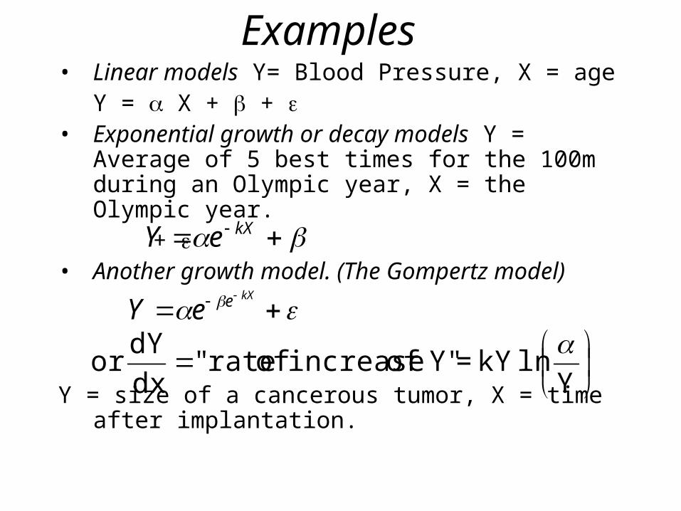
Examples • Linear models Y= Blood Pressure, X = age

Y = X + + • Exponential growth or decay models Y =

Average of 5 best times for the 100m during an Olympic year, X = the Olympic year.

+ • Another growth model. (The Gompertz model)

Y = size of a cancerous tumor, X = time after implantation.

kXeY

Yln kY = Y"of increase of rate"

dx

dYor

kXeeY

Note: the presence of the random error term, , (random noise).

This is a important term in any statistical model.

Without this term the model is deterministic and doesn’t require the statistical analysis

What is the value of these equations?

1.Equations give very precise and concise descriptions (models) of data and how dependent variables are related to independent variables.

2.The parameters of the equations usually have very useful interpretations relative to the phenomena that is being studied.

3.The equations can be used to calculate and estimate very useful quantities related to phenomena. Relative extrema, future or out-of-range values of the phenomena

4.Equations can provide the framework for comparison.

The Multiple Linear Regression Model

An important statistical model

Again we assume that we have a single dependent variable Y and p (say) independent variables X1, X2, X3, ... , Xp.

The equation (model) that generally describes the relationship between Y and the Independent variables is of the form:

Y = f(X1, X2,... ,Xp | 1, 2, ... , q) +

where 1, 2, ... , q are unknown parameters of the function f

and is a random disturbance (usually assumed to have a normal distribution with mean 0 and standard deviation .

In Multiple Linear Regression we assume the following model

Y = 0 + 1 X1 + 2 X2 + ... + p Xp +

This model is called the Multiple Linear Regression Model.

Again are unknown parameters of the model and where0, 1, 2, ... , p are unknown parameters and

is a random disturbance assumed to have a normal distribution with mean 0 and standard deviation .

The importance of the Linear model

1. It is the simplest form of a model in which each independent variable has some effect on the .dependent variable Y. When fitting models to data one tries to find the simplest form of a model that still adequately describes the relationship between the dependent variable and the independent variables. The linear model is sometimes the first model to be fitted and only abandoned if it turns out to be inadequate.

2. In many instances a linear model is the most appropriate model to describe the dependence relationship between the dependent variable and the independent variables. This will be true if the dependent variable increases at a constant rate as any or the independent variables is increased while holding the other independent variables constant.

3. Many non-Linear models can be put into the form of a Linear model by appropriately transforming the dependent variables and/or any or all of the independent variables. This important fact ensures the wide utility of the Linear model. (i.e. the fact the many non-linear models are linearizable.)

An Example

The following data comes from an experiment that was interested in investigating the source from which corn plants in various soils obtain their phosphorous. The concentration of inorganic phosphorous (X1) and the concentration of organic

phosphorous (X2) was measured in the soil of n = 18

test plots. In addition the phosphorous content (Y) of corn grown in the soil was also measured. The data is displayed below:

InorganicPhosphorous

X1

OrganicPhosphorous

X2

Plant Available

PhosphorousY

InorganicPhosphorous

X1

OrganicPhosphorous

X2

Plant Available

Phosphorous

Y

0.4 53 64 12.6 58 51

0.4 23 60 10.9 37 76

3.1 19 71 23.1 46 96

0.6 34 61 23.1 50 77

4.7 24 54 21.6 44 93

1.7 65 77 23.1 56 95

9.4 44 81 1.9 36 54

10.1 31 93 26.8 58 168

11.6 29 93 29.9 51 99

Coefficients

Intercept 56.2510241 (0)

X1 1.78977412 (1)

X2 0.08664925 (2)

Equation:

Y = 56.2510241 + 1.78977412 X1 + 0.08664925 X2

Summary of the Statistics used in

Multiple Regression

The Least Squares Estimates:

- The values that minimize

0, 1, 2, . . . , p

RSS n

i1

yi yi2

n

i1

yi 0 1xi1 2xi2 . . . pxip2 .

1110ˆ ppii xxy Note:

= predicted value of yi

The Analysis of Variance Table Entries

a) Adjusted Total Sum of Squares (SSTotal)

b) Residual Sum of Squares (SSError)

c) Regression Sum of Squares (SSReg)

Note:

i.e. SSTotal = SSReg +SSError

SSTotal n

i1

yi y_2. d.f. n 1

RSS SSError n

i1

yi yi2. d.f. n p 1

SSReg SS1,2, . . . , p n

i1

yi y_2. d.f. p

n

i1

yi y_2

n

i1

yi y_2

n

i1

yi yi 2 .

The Analysis of Variance Table

Source Sum of Squares d.f. Mean Square F

Regression SSReg p SSReg/p = MSReg MSReg/s2

Error SSError n-p-1 SSError/(n-p-1) =MSError = s2

Total SSTotal n-1

Uses: 1. To estimate 2 (the error variance).

- Use s2 = MSError to estimate 2.

2. To test the Hypothesis

H0: 1 = 1 = 2= ... = p = 0.

Use the test statistic

F = MSReg/ s2

= [(1/p)SSReg]/[(1/(n-p-1))SSError] .

- Reject H0 if F > Fa(p,n-p-1).

3. To compute other statistics that are useful in describing the relationship between Y (the dependent variable) and X1, X2, ... ,Xp (the independent variables).a) R2 = the coefficient of determination

= SSReg/SSTotal

=

= the proportion of variance in Y explained by

X1, X2, ... ,Xp

1 - R2 = the proportion of variance in Y

that is left unexplained by X1, X2, ... , Xp

= SSError/SSTotal.

ˆ y i y 2

i1

n

y i y 2

i1

n

b)Ra2 = "R2 adjusted" for degrees of freedom.

= 1 -[the proportion of variance in Y that is left

unexplained by X1, X2,... , Xp adjusted for d.f.]

= 1 - [(1/(n-p-1))SSError]/[(1/(n-1))SSTotal] .

= 1 - [(n-1)SSError]/[(n-p-1)SSTotal] .

= 1 - [(n-1)/(n-p-1)] [1 - R2 ].

c) R=R2 = the Multiple correlation coefficient of Y with X1, X2, ... ,Xp

=

= the maximum correlation between Y and a linear combination of X1, X2, ... ,Xp

Comment: The statistics F, R2, Ra2 and R are

equivalent statistics.

SSRe g

SSTotal

Using SPSS

Note: The use of another statistical package such as Minitab is similar to using SPSS

After starting the SSPS program the following dialogue box appears:

If you select Opening an existing file and press OK the following dialogue box appears

The following dialogue box appears:

If the variable names are in the file ask it to read the names. If you do not specify the Range the program will identify the Range:

Once you “click OK”, two windows will appear

One that will contain the output:

The other containing the data:

To perform any statistical Analysis select the Analyze menu:

Then select Regression and Linear.

The following Regression dialogue box appears

Select the Dependent variable Y.

Select the Independent variables X1, X2, etc.

If you select the Method - Enter.

All variables will be put into the equation.

There are also several other methods that can be used :

1. Forward selection

2. Backward Elimination

3. Stepwise Regression

Forward selection

1. This method starts with no variables in the equation

2. Carries out statistical tests on variables not in the equation to see which have a significant effect on the dependent variable.

3. Adds the most significant.

4. Continues until all variables not in the equation have no significant effect on the dependent variable.

Backward Elimination

1. This method starts with all variables in the equation

2. Carries out statistical tests on variables in the equation to see which have no significant effect on the dependent variable.

3. Deletes the least significant.

4. Continues until all variables in the equation have a significant effect on the dependent variable.

Stepwise Regression (uses both forward and backward techniques)

1. This method starts with no variables in the equation

2. Carries out statistical tests on variables not in the equation to see which have a significant effect on the dependent variable.

3. It then adds the most significant.

4. After a variable is added it checks to see if any variables added earlier can now be deleted.

5. Continues until all variables not in the equation have no significant effect on the dependent variable.

All of these methods are procedures for attempting to find the best equation

The best equation is the equation that is the simplest (not containing variables that are not important) yet adequate (containing variables that are important)

Once the dependent variable, the independent variables and the Method have been selected if you press OK, the Analysis will be performed.

The output will contain the following table

Model Summary

.822a .676 .673 4.46Model1

R R SquareAdjustedR Square

Std. Errorof the

Estimate

Predictors: (Constant), WEIGHT, HORSE, ENGINEa.

R2 and R2 adjusted measures the proportion of variance in Y that is explained by X1, X2, X3, etc (67.6% and 67.3%)

R is the Multiple correlation coefficient (the maximum correlation between Y and a linear combination of X1, X2, X3, etc)

The next table is the Analysis of Variance Table

The F test is testing if the regression coefficients of the predictor variables are all zero. Namely none of the independent variables X1, X2, X3, etc have any effect on Y

ANOVAb

16098.158 3 5366.053 269.664 .000a

7720.836 388 19.899

23818.993 391

Regression

Residual

Total

Model1

Sum ofSquares df

MeanSquare F Sig.


Dependent Variable: MPGb.

The final table in the output

Gives the estimates of the regression coefficients, there standard error and the t test for testing if they are zeroNote: Engine size has no significant effect on Mileage

Coefficientsa

44.015 1.272 34.597 .000

-5.53E-03 .007 -.074 -.786 .432

-5.56E-02 .013 -.273 -4.153 .000

-4.62E-03 .001 -.504 -6.186 .000

(Constant)

ENGINE

HORSE

WEIGHT

Model1

B Std. Error

UnstandardizedCoefficients

Beta

Standardized

Coefficients

t Sig.

Dependent Variable: MPGa.

The estimated equation from the table below:

Is:

Coefficientsa

44.015 1.272 34.597 .000

-5.53E-03 .007 -.074 -.786 .432

-5.56E-02 .013 -.273 -4.153 .000

-4.62E-03 .001 -.504 -6.186 .000

(Constant)

ENGINE

HORSE

WEIGHT

Model1

B Std. Error


Beta

Standardized

Coefficients

t Sig.


5.53 5.56 4.6244.0

1000 100 1000Mileage Engine Horse Weight Error

Note the equation is:

Mileage decreases with:

5.53 5.56 4.6244.0

1000 100 1000Mileage Engine Horse Weight Error

1. With increases in Engine Size (not significant, p = 0.432)With increases in Horsepower (significant, p = 0.000)With increases in Weight (significant, p = 0.000)

Properties of the Least Squares Estimators:

1. Normally distributed (If there error terms are Normally distributed)

2. Unbiased Estimators of the Linear Parameters 0, 1, 2, ... p.

3. Minimum Variance (Minimum Standard Error) of all Unbiased Estimators of the Linear Parameters 0, 1, 2, ... p.

0, 1, 2, . . . , p

Comments:

1. The Error Variance s2 (and s). 2. sXi, the standard deviation of Xi (the ith

independent variable).

3. The sample size n.

4. The correlations between all pairs of variables.

The standard error of i, S.E.i sˆ i depends on

• decreases as s decreases.• decreases as sXi increases.• decreases as n increases.• increases as the correlation between pairs of

independent variables increases.– In fact the standard error of the least squares

estimates can be extremely high if there is a high correlation between one of the independent variables and a linear combination of the remaining independent variables. (the problem of Multicollinearity).

The standard error of i, S.E.i sˆi

The Covariance Matrix,Correlation and XTX inverse matrix

The Covariance Matrix

S.E.02

Cov0, 1

S.E.12

. . .

. . .

Cov0, p

Cov1, p

. . .

S.E.p2

covi, j rij sˆ isˆ j

rijS.E.iS.E.j

where rij correlation between i andj.

where

and

The Correlation Matrix

r01

1

.. .

. . .

r0p

r1p

1

The XTX inverse matrix

a00

a01

a11

a0p

a1p

app

.

If we multiply each entry in the XTX inverse matrix by s2 = MSError this matrix turns into the covariance matrix for :

0, 1, 2, . . . , p

Thus S.E.i2 s2 aii and Covi, j s2 aij.

These matrices can be used to compute standard Errors for linear combinations of the regression coefficients

Namely

L c00 c11 cpp

ji

jiji

n

iiiL

ccEScsLES )ˆ,ˆcov(2)]ˆ.(.[ˆ..0

22ˆ

ji ijji

n

i ijii

ssrccsc ˆˆ0

2

ˆ

2 2

ji ijji

n

i iiiaccacs 2

0

2

S.E.i j si j S.E.i

2 S.E.j

2 2 1 1covi, j

S.E.i2 S.E.j

2 2 covi, j

s2i

s2j

2 rijsisj

s aii ajj 2aij

For example if L i j, then

An ExampleSuppose one is interested in how the cost per month

(Y) of heating a plant is determined the average atmospheric temperature in the Month (X1) and the number of operating days in the month (X2). The data on these variables was collected for n = 25 months selected at random and is given on the following page.

Y = cost per month of heating a plant X1 = average atmospheric temperature in the monthX2 = the number of operating days for the plant in the

month.

1 1098 35.3 20

2 1113 29.7 20

3 1251 30.8 23

4 840 58.8 20

5 927 61.4 21

6 873 71.3 22

7 636 74.4 11

8 850 76.7 23

9 782 70.7 21

10 914 57.5 20

11 824 46.4 20

12 1219 28.9 21

13 1188 28.1 21

14 957 39.1 19

15 1094 46.8 23

16 958 48.5 20

17 1009 59.3 22

18 811 70.0 22

19 683 70.0 22

20 888 74.5 23

21 768 72.1 20

22 847 58.1 21

23 886 44.6 20

24 1036 33.4 20

Month Y X1 X2

25 1108 28.6 22

The Least Squares Estimates:

Constant X1 X2

Estimate 912.6 -7.24 20.29

Standard Error 110.28 0.80 4.577

The Covariance Matrix

Constant X1 X2

Constant 12162 -49.203 -464.36

X1 .63390 .76796

X2 20.947

The Correlation Matrix

Constant X1 X2

Constant 1.000 -.1764 -.0920

X1 1.000 .0210

X2 1.000

The XTX Inverse matrix

Constant X1 X2

Constant 2.778747 -0.011242 -0.106098

X1 0.14207x10-3

0.175467x10-3

X2 0.478599

The Analysis of Variance Table

Source df SS MS F

Regression 2 541871 270936 61.899

Error 22 96287 4377

Total 24 638158

Summary Statistics

(R2, Radjusted2 = Ra

2 and R)

R2 = 541871/638158 = .8491

(explained variance in Y - 84.91 %)

Ra2 = 1 - [1 - R2][(n-1)/(n-p-1)]

= 1 - [1 - .8491][24/22]

= .8354 (83.54 %)

R = =.9215

= Multiple correlation coefficient

8491.

20 30 40 50 60 70 80

600

800

1000

1200

1400

TEMP

TSOC

10 15 20 25

600

800

1000

1200

1400

DAYS

TSOC

Three-dimensional Scatter-plot of Cost, Temp and Days.

Example

Motor Vehicle example

Variables

1. (Y) mpg – Mileage

2. (X1) engine – Engine size.

3. (X2) horse – Horsepower.

4. (X3) weight – Weight.

Select Analysis->Regression->Linear

To print the correlation matrix or the covariance matrix of the estimates select Statistics

Check the box for the covariance matrix of the estimates.

Here is the table giving the estimates and their standard errors.

Coefficientsa

44.015 1.272 34.597 .000

-5.53E-03 .007 -.074 -.786 .432

-5.56E-02 .013 -.273 -4.153 .000

-4.62E-03 .001 -.504 -6.186 .000

(Constant)

ENGINE

HORSE

WEIGHT

Model1

B Std. Error


Beta

Standardized

Coefficients

t Sig.


Coefficient Correlationsa

1.000 -.129 -.725

-.129 1.000 -.518

-.725 -.518 1.000

5.571E-07 -1.29E-06 -3.81E-06

-1.29E-06 1.794E-04 -4.88E-05

-3.81E-06 -4.88E-05 4.941E-05

WEIGHT

HORSE

ENGINE

WEIGHT

HORSE

ENGINE

Correlations

Covariances

Model1

WEIGHT HORSE ENGINE


Here is the table giving the correlation matrix and covariance matrix of the regression estimates:

What is missing in SPSS is covariances and correlations with the intercept estimate (constant).

This can be found by using the following trick

1. Introduce a new variable (called constnt)

2. The new “variable” takes on the value 1 for all cases

Select Transform->Compute

The following dialogue box appears

Type in the name of the target variable - constnt

Type in ‘1’ for the Numeric Expression

This variable is now added to the data file

Add this new variable (constnt) to the list of independent variables

Under Options make sure the box – Include constant in equation – is unchecked

The coefficient of the new variable will be the constant.

Here are the estimates of the parameters with their standard errors

Coefficientsa,b

-5.53E-03 .007 -.049 -.786 .432

-5.56E-02 .013 -.250 -4.153 .000

-4.62E-03 .001 -.577 -6.186 .000

44.015 1.272 1.781 34.597 .000

ENGINE

HORSE

WEIGHT

CONSTNT

Model1

B Std. Error


Beta

Standardized

Coefficients

t Sig.


Linear Regression through the Originb.

Note the agreement with parameter estimates and their standard errors as previously calculated.

Here is the correlation matrix and the covariance matrix of the estimates.

Coefficient Correlationsa,b

1.000 .761 -.318 -.824

.761 1.000 -.518 -.725

-.318 -.518 1.000 -.129

-.824 -.725 -.129 1.000

1.619 6.808E-03 -5.43E-03 -7.82E-04

6.808E-03 4.941E-05 -4.88E-05 -3.81E-06

-5.427E-03 -4.88E-05 1.794E-04 -1.29E-06

-7.821E-04 -3.81E-06 -1.29E-06 5.571E-07

CONSTNT

ENGINE

HORSE

WEIGHT

CONSTNT

ENGINE

HORSE

WEIGHT

Correlations

Covariances

Model1

CONSTNT ENGINE HORSE WEIGHT


Linear Regression through the Originb.

Testing for Hypotheses related to

Multiple Regression.

Testing for Hypotheses related to Multiple Regression.

The General Linear Hypothesis

H0: h111 + h122 + h133 +... + h1pp = h1

h211 + h222 + h233 +... + h2pp = h2

...

hq11 + hq22 + hq33 +... + hqpp = hq

where h11h12, h13, ... , hqp and h1h2, h3, ... , hq are known coefficients.

Examples 1. H0: 1 = 0

2. H0: 1 = 0, 2 = 0, 3 = 0

3. H0: 1 = 2

4. H0: 1 = 2 , 3 = 4

5. H0: 1 = 1/2(2 + 3)

6. H0: 1 = 1/2(2 + 3), 3 = 1/3(4 + 5 + 6)

1. The Complete Model

Y = 0 + 1X1 + 2X2 + 3X3 +... + pXp+

2. The Reduced Model

The model implied by H0.

You are interested in knowing whether the complete model can be simplified to the reduced model.

When testing hypotheses there are two models of interest.

Some Comments1. The complete model contains more parameters and will

always provide a better fit to the data than the reduced model.

2. The Residual Sum of Squares for the complete model will always be smaller than the R.S.S. for the reduced model.

3. If the reduction in the R.S,S. is small as we change from the reduced model to the complete model, the reduced model should be accepted as providing an adequate fit.

4. If the reduction in the R.S,S. is large as we change from the reduced model to the complete model, the reduced model should be rejected as providing an adequate fit and the complete model should be kept.

These principles form the basis for the following test.

Testing the General Linear Hypothesis

The F-test for H0 is performed by carrying out two runs of a multiple regression package.

Run 1: Fit the complete model.

Resulting in the following Anova Table:

Source df Sum of Squares

Regression p SSReg

Residual (Error) n-p-1 SSError

Total n-1 SSTotal

Run 2: Fit the reduced model (q parameters eliminated)

Resulting in the following Anova Table:

Source df Sum of Squares

Regression p-q SS1Reg

Residual (Error) n-p+q-1 SS1Error

Total n-1 SSTotal

The Test:

The Test is carried out using the Test Statistic

where SSH0 = SS1

Error- SSError= SSReg- SS1Reg

and s2 = SSError/(n-p-1).

1 Reduction in the Residual Sum of Squares

Residual Mean Square for Complete modelqF

0

1

2

Hq SS

s

The test statistic, F, has an F-distribution with 1 = q d.f. in the numerator and 2 = n – p - 1 d.f. in the denominator if H0 is true.

Distribution when H0 is true

0

0.1

0.2

0.3

0.4

0.5

0.6

0.7

0 1 2 3 4 5

The Critical Region

Reject H0 if F > F(q, n – p – 1)

F(q, n – p – 1)

The Anova Table for the Test:

Source df Sum of Squares Mean Square F

Regression p-q SS1Reg [1/(p-q)]SS1

Reg MS1Reg/s2

(for the

reduced model)

Departure q SSH0 (1/q)SSH0 MSH0/s2

from H0

Residual n-p-1 SSError s2

(Error)

Total n-1 SSTotal

Some Examples:Four independent Variables

X1 , X2 , X3, X4

The Complete Model

Y = 0 + 1X1 + 2X2 + 3X3 + 4X4+

1) a) H0: 3 = 0, 4 = 0 (q = 2)

b) The Reduced Model:

Y = 0 + 1X1 + 2X2 +

Dependent Variable: Y

Independent Variables: X1 , X2

2) a) H0: 3 = 4.5, 4 = 8.0 (q = 2)

b) The Reduced Model:

Y – 4.5X3 – 8.0X4 = 0 + 1X1 + 2X2 +

Dependent Variable: Y – 4.5X3 – 8.0X4

Independent Variables: X1 , X2

Example

Motor Vehicle example

Variables

1. (Y) mpg – Mileage

2. (X1) engine – Engine size.

3. (X2) horse – Horsepower.

4. (X3) weight – Weight.

Suppose we want to test:

H0: 1 = 0 against HA: 1 ≠ 0

i.e. engine size(engine) has no effect on mileage(mpg).

The Full model:

Y = 0 + 1 X1 + 2 X2 + 1 X3 + (mpg) (engine) (horse) (weight)

The reduced model:

Y = 0 + 2 X2 + 1 X3 +

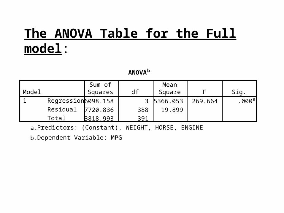
The ANOVA Table for the Full model:

ANOVAb

16098.158 3 5366.053 269.664 .000a

7720.836 388 19.899

23818.993 391

Regression

Residual

Total

Model1

Sum ofSquares df

MeanSquare F Sig.



The reduction in the residual sum of squares

= 7733.138452 - 7720.835649 = 12.30280251

ANOVAb

16085.855 2 8042.928 404.583 .000a

7733.138 389 19.880

23818.993 391

Regression

Residual

Total

Model1

Sum ofSquares df

MeanSquare F Sig.

Predictors: (Constant), WEIGHT, HORSEa.


The ANOVA Table for the Reduced model:

The ANOVA Table for testing

H0: 1 = 0 against HA: 1 ≠ 0

Sum of Squares df Mean Square F Sig.Regression 16085.85502 2 8042.927509 404.18628 0.0000

1 = 0 12.30280251 1 12.30280251 0.6182605 0.4322 Residual 7720.835649 388 19.89906095Total 23818.99347 391

1 = 0

Now suppose we want to test:

H0: 1 = 0, 2 = 0 against HA: 1 ≠ 0 or 2 ≠ 0

i.e. engine size (engine) and horsepower (horse) have no effect on mileage (mpg).

The Full model:

Y = 0 + 1 X1 + 2 X2 + 1 X3 + (mpg) (engine) (horse) (weight)

The reduced model:

Y = 0 + 1 X3 +

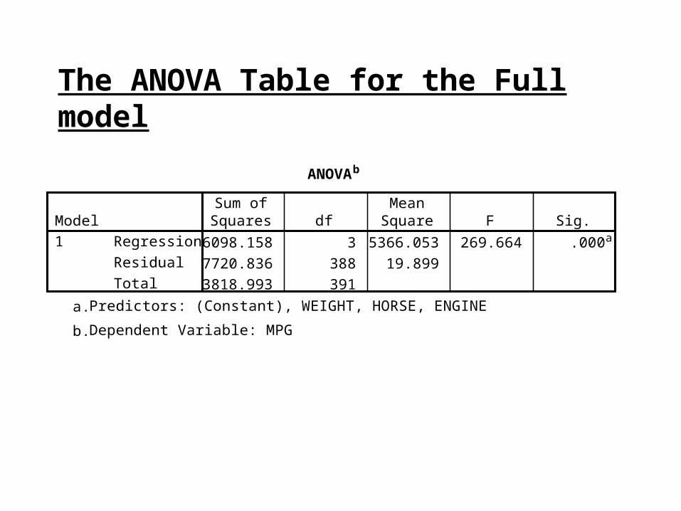
The ANOVA Table for the Full model

ANOVAb

16098.158 3 5366.053 269.664 .000a

7720.836 388 19.899

23818.993 391

Regression

Residual

Total

Model1

Sum ofSquares df

MeanSquare F Sig.



The reduction in the residual sum of squares

= 8299.023 - 7720.835649 = 578.1875392

The ANOVA Table for the Reduced model:

ANOVAb

15519.970 1 15519.970 729.337 .000a

8299.023 390 21.280

23818.993 391

Regression

Residual

Total

Model1

Sum ofSquares df

MeanSquare F Sig.

Predictors: (Constant), WEIGHTa.


The ANOVA Table for testing

H0: 1 = 0, 2 = 0 against HA: 1 ≠ 0 or 2 ≠ 0

Sum of Squares df Mean Square F Sig.Regression 15519.97028 1 15519.97028 779.93481 0.0000

1 = 0, 2 = 0 578.1875392 2 289.0937696 14.528011 0.0000 Residual 7720.835649 388 19.89906095Total 23818.99347 391

1 = 0, 2 = 0

Testing the General Linear Hypothesis

Another Example

In the following example:

Weight Gain was being measured along with the amount of protein in the diet due to the following sources

– Beef,

– Pork, and

– two types of cereals.

Dependent Variable

Y = Weight Gain

Independent Variables

X1 = the amount of protein in the diet due to the Beef

source,

X2 = the amount of protein in the diet due to the Pork

source,

X3 = the amount of protein in the diet due to the

Cereal 1 source

X4 = the amount of protein in the diet due to the

Cereal 2 source.

The Multiple Linear model

Y = 0 + 1 X1 + 2 X2 + 3 X3 + 4 X4 +

or

Weight Gain = 0 + 1 (Beef)

+ 2 (Pork)

+ 3 (Cereal 1)

+ 4 (Cereal 2) +

case Beef Pork Cereal 1 Cereal 2 Weight Gain1 3.48 8.95 9.26 4.72 43.052 1.77 4.93 2.77 0.45 34.293 6.39 3.01 4.92 1.79 31.794 9.97 0.67 8.56 8.42 41.945 7.41 4.19 8.41 4.43 45.296 3.58 4.1 2.05 1.1 32.027 1.2 2.64 6.03 5.55 26.938 6.8 0.97 4.8 5.98 36.459 2.3 9.95 0.89 6.74 31.52

10 6.47 0.6 9.17 7.27 39.6711 5.08 4.98 8.65 3.24 37.7212 0.62 2.24 7.79 0.08 29.0113 6.47 2.19 2.5 3.08 31.1514 7.35 0.18 0.67 7.87 31.89

The weight gains are given in the following table below:

The Summary Statistics of Regression computation are given below:

Regression Statistics

Multiple R 0.89243188

R Square 0.79643465

Adjusted R Square 0.70596117

Standard Error 3.03382552

Observations 14

The estimates of the regression coefficients and their standard errors are given below:

Coefficients Standard Error

t Stat P-value Lower 95% Upper 95%

Intercept 19.4614989 2.9165956 6.67267651 9.1339E-05 12.8636963 26.0593016

X11.47769633 0.41288474 3.57895604 0.00594044 0.54368545 2.41170721

X20.97584224 0.32968801 2.95989606 0.01596221 0.23003558 1.7216489

X30.94351642 0.26479013 3.56326123 0.00608811 0.34451907 1.54251378

X4-0.0344526 0.36188355 -0.0952035 0.92623923 -0.8530907 0.78418551

ANOVA

df SS MS F Significance F

Regression 4 324.093267 81.0233168 8.8029618 0.00355147

Residual 9 82.8368756 9.20409729

Total 13 406.930143

Note that i is the rate of increase in weight

gain due to increase in protein with respect to the given source of protein. One of course would be interested in whether weight gain increased with protein for any of the sources of protein. That is testing the Null Hypothesis

H0: 1 = 0 , 2 = 0, 3 = 0 and 4 = 0

against the alternative Hypothesis HA: at least one i 0.

This can be achieved by using the Anova Table below:


Regression 4 324.093267 81.0233168 8.8029618 0.00355147

Residual 9 82.8368756 9.20409729

Total 13 406.930143

Test statistic – F ratio

F distribution

Significance – p value

F

• F distribution describes the behaviour or the F statistics when H0 is true.

• If associated p-value is small, H0 should be rejected in favour of HA.

• The cut-off values are = .05 or = .01

However one would also be interested in making more specific comparisons.

Namely, comparing effect on weight gain of – the two meat sources

and – the two cereal sources

on weight gain

In this case we would be interested in testingthe Null Hypothesis

H0: 1 = 2, 3 = 4 against

the alternative Hypothesis HA: 1 2 or 3 4.

Then assuming

H0: 1 = 2 , 3 = 4

the reduced model becomesY = 0 + 1 (X1 + X2) + 3 (X3 + X4) + Dependent Variable: YIndependent Variables: (X1 + X2) and

(X3 + X4)

The Anova Table for the reduced model:


Regression 2 276.132469 138.066235 11.6112813 0.0019451

Residual 11 130.797674 11.8906976

Total 13 406.930143

The Anova Table for the complete model:


Regression 4 324.093267 81.0233168 8.8029618 0.00355147

Residual 9 82.8368756 9.20409729

Total 13 406.930143

the Anova Table to carrying out the test:


1 + 2= 0 , 3 + 4 = 0 2 276.132469 138.066235 15.0005188 0.00136222

1 = 2 , 3 = 4 2 47.9607982 23.9803991 2.60540478 0.12802848

Residual 9 82.8368756 9.20409729

Total 13 406.930143

DUMMY VARIABLES

fitting equations to data. a common situation: suppose that we have a single dependent variable y...

Documents