Journal of Policy Modeling 39 (2017) 99–113

Available online at www.sciencedirect.com

ScienceDirect

Fiscal sustainability in an emerging market economy:When does public debt turn bad?

Ahmad Zubaidi Baharumshah a,b,∗, Siew-Voon Soon b, Evan Lau c

a Financial Economics Research Centre, Faculty of Economics and Management, Universiti Putra Malaysia, 43400UPM Serdang, Selangor, Malaysia

b Department of Economics, Faculty of Economics and Management, Universiti Putra Malaysia, 43400 UPM Serdang,Selangor, Malaysia

c Department of Economics, Faculty of Economics and Business, Universiti Malaysia Sarawak (UNIMAS), 94300 KotaSamarahan, Sarawak, Malaysia

Received 23 March 2016; received in revised form 20 September 2016; accepted 21 October 2016Available online 24 November 2016

Abstract

This paper proposes a Markov-switching model to assess the sustainability of fiscal policy in Malaysiafor the period 1980–2014. Our results indicate the policymakers in the past have followed a sustainablefiscal policy, except during the brief periods of economic difficulty. The empirical analysis reveals that thegovernment should cut the deficits only if they exceed a certain level, to ensure their sustainability in thelong-run. Specifically, we find that after public debt exceeds a certain threshold level (above 55% of the grossdomestic product), it is negatively correlated with economic activity. In addition to the threshold effect, weconfirm the presence of a unidirectional causal relation between debt and growth.© 2016 The Society for Policy Modeling. Published by Elsevier Inc. All rights reserved.

JEL classification: E62; F34; H63

Keywords: Endogenous multiple breaks; Fiscal sustainability; Debt; Economic growth

1. Introduction

One of the most challenging issues faced by both developed and developing countries in recentyears are dealing with the accumulation (size) of public debt. A build-up of public debt can

∗ Corresponding author. Fax: +603 89486188.E-mail addresses: baharumshah@yahoo.com, zubaidi@upm.edu.my (A.Z. Baharumshah).

http://dx.doi.org/10.1016/j.jpolmod.2016.11.0020161-8938/© 2016 The Society for Policy Modeling. Published by Elsevier Inc. All rights reserved.

100 A.Z. Baharumshah et al. / Journal of Policy Modeling 39 (2017) 99–113

adversely affect economic progress through several channels (higher long-term interest rates,higher taxation, greater uncertainty, vulnerability to crises, etc.), especially when their levelexceeds a certain threshold. In addition, fiscal sustainability is most likely to be aggravated inthose countries experiencing debt distress. On the contrary, a low level of public debt allows thefiscal policy to play more of a stabilizing role during economic downturns and dampens, or at leastdoes not exacerbate, economic cycles.1 Maintaining fiscal sustainability is important to obtainenough “fiscal space” for orderly adjustments to mitigate the impacts of financial crises. Therecent global financial crisis (GFC) is a case in point. A sustainable debt ratio is one such that thegovernment has no incentive to default on its internal debt. From another perspective, the notionof sustainability implies that there is a limit to the flexibility of fiscal policy as a stabilizationpolicy tool.

This paper has two main objectives. The first is to examine the sustainability of fiscal policyover the period from 1980:Q1 to 2014:Q3, including the Asian financial crisis (AFC) and therecent GFC.2 The usual approach applied to investigate the behavior of a nation’s fiscal stance isbased on the intertemporal budget constraint (IBC) of the government (Mahdavi & Westerlund,2011). Fiscal policy is considered sustainable if it satisfies the IBC in present-value terms—thatis, the current level of debt equals the present discounted value of primary surpluses. To examinethe sustainability of budget deficits, many researchers rely on the evidence from unit-root tests ofwhich rejection imply sustainability.3 Adding to concerns about fiscal deficits is the fear that publicdebts have reached levels that might hinder economic growth and the starting of a debt, growthand high employment vicious circle. It is widely accepted that, with a moderate level of publicdebt, fiscal policy can induce economic growth, but at high levels of public debt, the expectedtax increases will mitigate the positive results of the fiscal outcome, decreasing investment andconsumption, reducing employment, and lowering growth rates of the gross domestic product(GDP).4 Since the subprime crisis that began in the US in 2007, many countries around the worldhave found themselves with high ratios of debt-to-GDP. These are due to high budget deficitsas a result of declining tax revenue and rising public spending due to economic slowdown. Intimes like these, the central question that arises concerns the relationship between public debt andeconomic growth. Specifically, we try to provide an answer whether fiscal policy has a Keynesianor non-Keynesian effects on economic activity.

Like the other Asian countries, Malaysia is concerned about the large debts as they couldderail the sound economic growth experienced before the GFC. This brings us to the secondobjective of the study—that is, to investigate the existence of a threshold level of public debt in

1 By comparing the 1980s with the 1990s, Pattillo, Poirson, and Ricci (2002) observed that economic growth for thepanel of 98 developing countries (Malaysia included) declined during the early period when total debt was accumulatingbut accelerated during the 1990s when debt reduction occurred.

2 During the AFC, the region suffered a massive reversal of capital inflows as investor confidence in the region fall.During the GFC, financial institutions in the US and Europe, withdrew their funds from Asia in order to support theirbadly damaged balance sheet at home.

3 Most of the analysis conducted in the past has in fact provided mixed results. The outcome of these tests depends onthe length of sample period and whether breaks are accounted for to account for the financial crisis and the slowing downof economic activities, among other things; see Baharumshah and Lau (2007) and articles cited therein.

4 High levels of debt may place serious constraints on a nation’s ability to conduct countercyclical policies and thusincrease output volatility and reduce economic growth. However, the relationship between debt and the ability to conductcountercyclical policy is more likely to depend on the composition of public debt rather than on the level of public debt.Therefore, countries with different debt structures and monetary arrangements are likely to start facing problems at verydifferent levels of debt.

A.Z. Baharumshah et al. / Journal of Policy Modeling 39 (2017) 99–113 101

the debt-growth nexus and the effect of the tipping point(s) on economic growth. Reinhart andRogoff (2010), whose work has garnered a great deal of attention, alluded to debt ratios above90% (60%) as detrimental to economic growth for the advanced countries (emerging marketeconomies).5 Their work was based on a large set of countries, which had major variations inthe quality of their economic and political institutions.6 A number of studies that followed thisseminal paper to investigate the debt-growth nexus broadly confirmed their findings, showing thatthe turning point beyond which debt sharply slows economic growth is a ratio of around 90%;see Cecchetti, Mohanty, and Zampolli (2011, 85% of GDP) for member countries of the Orga-nization for Economic Cooperation and Development (OECD) and Baum, Checherita-Westphal,and Rother (2013, 95% of GDP) for the Eurozone countries. To further support their empiricalfindings, Baum et al. (2013) showed that interest rates are subject to increased pressure when thedebt-to-GDP ratio rises above 70% level.

Our research is closely related to Caner, Grennes, and Koehler-Geib (2010) and Égert (2015),who based their empirical analysis on a threshold regression. Caner et al. (2010) apply a two-regime model developed by Hansen (1999, 2000) and found that the negative nonlinear correlationbetween debt and economic growth kicks in when the public debt level in 101 countries is around77% of debt-to-GDP ratio.7 According to these authors, the effect more pronounced in the devel-oping economies, including Malaysia (threshold is around 64%). Égert (2015) conducted a similarstudy, but finds that in very rare cases when the nonlinearity like that in Reinhart and Rogoff (2010)can be detected. Égert (2015) also provides a lower threshold band (between 20% and 60%) forpublic debt, which clearly excludes the point estimates reported in some of the earlier studies.They conclude by pointing out that the nonlinear effects might be more complex and difficult tomodel than previously thought (p. 238). Whether there is a tipping point in the level of public debtabove which a nation’s economic progress is dramatically compromised is critically important todetermine because of its implications for debt accumulation. If there is no such clear thresholdlevel, and the evidence suggests that weak growth causes high debt, rather than the other wayaround, then higher priority should be placed on increasing growth, rather than on reducing debtlevel. Such a conclusion would indicate that much less fiscal austerity is appropriate to attainsustainable growth in the aftermath of GFC.

This paper differs from previous literature in the following ways: First, we apply a Markov-switching nonlinear framework to test for fiscal sustainability. The sheer size of the deficits duringthat period contributed to justifiable concern about sustainability.8 This approach allows not onlyfor shifts in the mean but also the variance in the series being examined. The methodology allowsus to determine whether the government debt-to-GDP ratio is stationary after considering majorregime shifts in the data generating process. Second, we apply a threshold regression using public

5 Cecchetti et al. (2011) and Checherita and Rother (2010) found that the negative correlation between debt and growthbecomes particularly stronger when debt level approaches 100% of GDP. The threshold level also referred to as “tippingpoint” has received much attention in recent years because many countries have reached or expected to cross this point innear future.

6 Their analysis was based on descriptive statistics. For the emerging market economies, the analysis reveals that whenthe debts exceed the threshold of 90%, GDP growth rate drops by two percentage points. While Reinhart and Rogoff(2010) and others consider a one threshold model, our study provides a complementary evidence based on two thresholds.

7 For a recent survey of studies on the public debt-growth nexus, see Mitze and Matz (2015).8 If the interest rate is higher than the growth rate of GDP, the ratio of debt-to-GDP will tend to rise and poses serious

challenges, while if it is lower, the debt will tend to decline, for a given level of the primary balance. Narayanan (2012)pointed out that the growth of debt has outpaced the growth of GDP, suggesting that economic growth (after 1997 crisis)has been unable to absorb the increasing debt.

102 A.Z. Baharumshah et al. / Journal of Policy Modeling 39 (2017) 99–113

debt as threshold variable to show economic growth is negatively affected when the debt levelexceeds a certain tipping point(s). Unlike previous studies, the empirical analysis allows for threeregimes.9 Third, we test the causality interplay of debt-growth nexus and answer the questionof when the debt goes bad for the Malaysian economy. We also depart from previous studiesby formally showing that public debt Granger cause economic growth and not vice versa. Thelatter finding implies that expansionary fiscal policies that increase in the level debt (above thetipping point(s)) may reduce economic growth, and hence partly negate the positive effects offiscal stimulus.10

The rest of this paper organized as follows. Section 2 briefly reviews the theoretical frame-work. Section 3 discusses the statistical strategy utilized in the analysis. The empirical resultsare interpreted in the following section, and the final section contains the conclusion and policyimplications of this study.

2. Fiscal sustainability hypothesis

An approach to fiscal sustainability can be presented as follows, called the Government BudgetIdentity (GBI):11

Gt + (1 + rt)Debtt−1 = Rt + Debtt, (1)

where Gt is the level of government primary expenditure, rt is the interest rate, Rt is the level ofgovernment revenue, and Debtt is the debt level at time t = 1,. . .,T. Therefore, the level of debtcan be expressed as Debtt = φt(Rt+1 − Gt+1 + Debtt+1), where φt = (1 + rt+1)−1. By repeatingsubstitutions, assuming a constant future interest rate and solving forward, the IBC can be derived,which is equivalent to the expected present value constraint: Debtt = ∑∞

i=1φiEt(Rt+i − Gt+i),

which will hold as long as the limn→∞φnEt(Debtt+n) = 0 (transversality condition) is satisfied. In

other words, public debt is sustainable if the government does not engage in a Ponzi scheme.The integrated property of the debt ratio is highly debated in the literature. Some studies (e.g.,Ahmed & Rogers, 1995; Chen, 2014; Hamilton & Flavin, 1986; Holmes, Otero, & Panagiotidis,2010) investigate the time series property of the fiscal indicators. However, Bohn (2007) arguesthat the use of purely time series methods (e.g., a unit-root test) to test sustainability is invalid.In particular, the author claims that any order of integration of debt is in fact consistent with thetransversality condition. Eq. (1) can be rearranged and presented as the responsiveness of primarysurplus to the debt-GDP level as:

(R − G)tGDPt

= (i − g)Debtt−1

GDPt−1, (2)

9 Earlier studies relied on spline functions (e.g., Pattillo et al., 2002) or histograms (Reinhart & Rogoff, 2010) todetermine the threshold level. The only study we are aware of using a two thresholds model for testing the debt-growthnexus is Baum et al. (2013) but for a set of European Union countries.10 In this paper, we do not address the issue whether fiscal expansions always lead to an increase in debt. For a more

discussion on this point; see DeLong and Summers (2012).11 A majority of the theoretical discussion is taken from Byrne, Fiess, and MacDonald (2011, p. 139).

A.Z. Baharumshah et al. / Journal of Policy Modeling 39 (2017) 99–113 103

where g is the growth rate of nominal GDP. Accordingly, the budget balance response functioncan be expressed as:

(R − G)tGDPt

= β1 + β2Debtt

GDPt

+ ut. (3)

The expected sign for β2 is positive, which indicates fiscal probity on the part of the government.Any increase in debt is reflected in an increase in the government balance, that is, evidence of thesustainability of the implemented fiscal policy path. Rising debt ratios lead to a higher primarysurplus/GDP, which exerts a tendency toward mean reversion.

3. Methodology and data description

Recent literature has recognized that borrowing (debts) variables do not follow a linear path(Dogan & Bilgili, 2014; Raybaudi, Sola, & Spagnolo, 2004; Wagner & Elder, 2005).12 Theswitching regression approach was popularized by Hamilton (1989), applying a two-regimeautoregression to the quarterly growth rate in the real US gross national product, in whichthe regimes exogenously switched according to an unobserved Markov process. Because taxrevenue clearly depends on GDP, it seems logical to estimate a switching regression for tax rev-enue. By permitting switching between these N regimes, in which the dynamic behavior of theseries is markedly different, more complex dynamic patterns can be characterized. The switch-ing mechanism is controlled by an unobservable state variable that follows a first-order Markovchain.13

Following Hamilton (1989), we use Markov-switching intercept autoregressive heteroskedas-ticity error correction model (MSIAH-ECM) to test the sustainability of fiscal policy. The MSIAHmodel considers a full parameter shift as well as the change in the variance of the residuals. Specif-ically, the particular feature of this model is that it allows for different behavior in different statesof nature. The model with switching in the mean, error variance, and the coefficients of exogenousregressors is presented as:

�(R − G)tGDPt

= α1(st) +q∑

i=1

α2i(st)�

(R − G

GDP

)t−i

+q∑

i=0

α3i(st)�

(Debt

GDP

)t−i

+λ(st)ECTt−1 + ut, (4)

where � is the difference operator, ECTt−1 refers to a coefficient error correction term thatmeasures the speed of adjustment toward the long-run equilibrium, and st is the random variabledenoting the regime (unobserved random variable) with ut∼N[0, σ2(st)]. The st is followinga Markov chain defined by transition probabilities among the N states. The error correctioncoefficient is expected to carry a statistically significant negative sign if the variable returns to a

12 Focusing on the current account deficits for several countries (e.g., Japan, Brazil and US), Raybaudi et al. (2004) claimthat, even though one state could be associated with untenable (unsustainable) trade policy, the overall debt process maybe still sustainable, depending on the duration of the states and on the values of the parameter estimates of the switchingmodel. Similarly, Dogan and Bilgili (2014) conclude that public borrowing (external debt) and economic growth do notfollow a linear path but notice the nonlinearities effects of public borrowing on growth.13 The basic advantage of the Markov-switching process is the features such as the persistence of extreme observations

and the nonlinearity and having the ability to take into account the asymmetry of time series.

104 A.Z. Baharumshah et al. / Journal of Policy Modeling 39 (2017) 99–113

long-run equilibrium. The coefficient of λ in Eq. (4) is of interest because if λ = 0, then therewould be no long-run relationship among the variables.

The model is evaluated using the filtering procedure of Hamilton (1990), followed by thesmoothing algorithm proposed by Kim (1994). The transition probabilities are estimated thatgovern the movement from one regime to another. For instance, the probability of moving fromstate j in one period to state i in the next depends only on the previous state, as pi|j = P[st+1 =i|st = j], i, j = 0, ...N − 1. The full matrix of transition probabilities P is P = pi|j , with condi-tional probabilities in columns summing to one. The models are estimated up to q lags, whichare determined using model selection criteria, and varying the regime allows different dynamicswithin each regime. The number of regimes is chosen based on model selection criteria. Feasiblesequential quadratic programming in Lawrence and Tits (2001) is used for a maximization methodto ensure that the parameters stay within the feasible region.

Following Kim and Lima (2010), the half-life property of local persistence is obtained as:

h0.50 = ln(0.5b(1))/(−1/nd), (5)

where d = − ln(1 − λ)/ ln(n), b(1) = 1 − ∑kj=1λ

∗j−1 is the correction factor, λ is obtained from

the MSIAH-ECM, and n is the number of observations. Under the local-to-unity model, that iswhen the parameter is locally persistent, the half-life goes to infinity at a rate n. However, thehalf-life of the locally persistent model is always less than the local-to-unity model for a givenn. Thus, the local persistence process allows a speed of convergence that is not allowed by alocal-to-unity approximation, even when d is close to unity.

As elaborated in Phillips, Moon, and Xiao (2001), the local persistence process yields thestandard Central Limit Theorem. Using the delta method, the 95% confidence intervals (CIs) aregiven by:

h0.50 ± 1.96se(λ)([− ln 0.5/λ][ln(λ)]−2

), (6)

where se(λ) = √2/(n

12 + d

2 ). If d is between 0 and 1, the series is considered to be a standardizedlocal persistence process. As illustrated in Kim and Lima (2010), the series is a special case ofa local-to-unity process, as proposed by Rossi (2005), when d = 1; if d = 0, then the time seriesprocess has a short-memory dynamic.

This empirical analysis covers quarterly data over the period 1980:Q1 to 2014:Q3 (139 obser-vations). The data for debt (total debt, external debt, domestic debt) and the budget balance (thedifference between government revenue and government expenditure) come from Bank NegaraMalaysia (BNM) and the Malaysian Ministry of Finance.

4. Empirical results and discussions

Table 1 provides descriptive statistics for the variables used. The median (and mean) level ofdomestic debt is higher than it is for external debt. Those debt variables are unstable relative to thebudget balance, as suggested by the higher standard deviations. The analysis begins by examiningthe persistence in the variables of interest. To this end, we conduct an augmented Dickey–Fullerunit-root test. The unit-root test statistics for all series fail to reject the unit-root null, except forbudget balance at the 10% significance level. Hence, the unit-root tests suggest that Malaysia’sfiscal stance does not satisfy the IBC over the sample period considered and the fiscal authorityhas to change the course of its fiscal policy. Many earlier papers find evidence of structural breaks

A.Z. Baharumshah et al. / Journal of Policy Modeling 39 (2017) 99–113 105

Table 1Descriptive statistics, 1980:Q1-2014:Q3 (in percentage of GDP).

Mean Median Max. Min. SD Skewness Kurtosis ADF

Domestic debt 42.770 40.546 70.785 26.418 11.618 0.619 2.486 −2.481 (8)External debt 11.352 7.344 36.466 1.503 9.911 1.012 2.741 −1.603 (5)Total debt 54.122 48.654 100.719 29.633 19.655 0.957 2.707 −2.128 (4)Government revenue 5.732 5.693 8.354 3.148 1.082 0.105 2.836 −1.639 (9)Government expenditure 6.831 6.316 15.410 2.868 2.421 1.044 4.109 −2.565 (11)Budget balance, (R-G) −1.100 −0.857 2.382 −7.322 1.909 −0.985 4.276 −2.718* (11)

Notes: * indicates significant at the 10% level. Max and min refer to maximum and minimum value, respectively. SDindicates the standard deviation of the series, and ADF is the augmented-Dickey Fuller unit-root test. The values inparentheses refer to length lag selected based on modified Akaike information criterion. The critical value for unit-roottest at 1% = −3.481, 5% = −2.884, and 10% = 2.579.

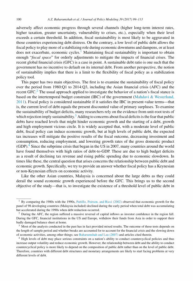
0.0

0.2

0.4

0.6

0.8

1.0

94 96 98 00 02 04 06 08 10 12 14

Debt (R-G)

GlobalFinancialCrisis

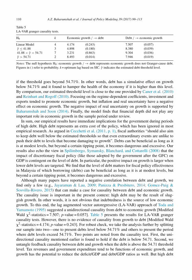
Fig. 1. Dynamics of fiscal policy persistence based on 15-year rolling window against the end year of sample period.

and nonlinearities in the debt process (Quintos, 1995). This means that to test for sustainability,we have to apply models that are equipped to handle these issues.

We further analyze the dynamics of fiscal policy deviation persistence in 15-year rollingwindow estimates against the end year of the sample period. We adopt the model by Phillipset al. (2001) using a 15-year (1980:Q1 to 1994:Q4) sample period. Four quarterly observations(1995:Q1 to 1995:Q4) are then added to re-estimate the persistence parameter. This one-yearincrement is repeated until the end of the sample period (2014:Q3).14 Fig. 1 displays the 15-yearrolling window estimates of the persistence parameter for total debt levels and the deficits thatproduce them. An interesting pattern emerged from this analysis, especially after the 2008 GFC.

14 It should be noted the first 15 years of our sample period are characterized by high but declining fiscal deficits. Thesecond period is characterized by growing deficits and increasing public debts.

106 A.Z. Baharumshah et al. / Journal of Policy Modeling 39 (2017) 99–113

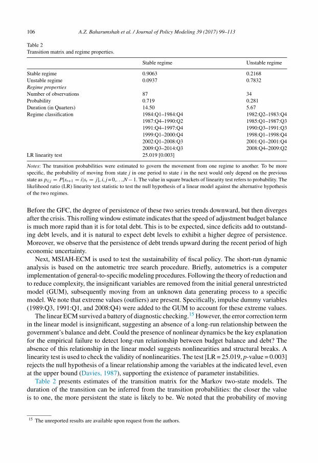
Table 2Transition matrix and regime properties.

Stable regime Unstable regime

Stable regime 0.9063 0.2168Unstable regime 0.0937 0.7832Regime propertiesNumber of observations 87 34Probability 0.719 0.281Duration (in Quarters) 14.50 5.67Regime classification 1984:Q1–1984:Q4 1982:Q2–1983:Q4

1987:Q4–1990:Q2 1985:Q1–1987:Q31991:Q4–1997:Q4 1990:Q3–1991:Q31999:Q1–2000:Q4 1998:Q1–1998:Q42002:Q1–2008:Q3 2001:Q1–2001:Q42009:Q3–2014:Q3 2008:Q4–2009:Q2

LR linearity test 25.019 [0.003]

Notes: The transition probabilities were estimated to govern the movement from one regime to another. To be morespecific, the probability of moving from state j in one period to state i in the next would only depend on the previousstate as pi|j = P[st+1 = i|st = j], i, j = 0,. . .,N − 1. The value in square brackets of linearity test refers to probability. Thelikelihood ratio (LR) linearity test statistic to test the null hypothesis of a linear model against the alternative hypothesisof the two regimes.

Before the GFC, the degree of persistence of these two series trends downward, but then divergesafter the crisis. This rolling window estimate indicates that the speed of adjustment budget balanceis much more rapid than it is for total debt. This is to be expected, since deficits add to outstand-ing debt levels, and it is natural to expect debt levels to exhibit a higher degree of persistence.Moreover, we observe that the persistence of debt trends upward during the recent period of higheconomic uncertainty.

Next, MSIAH-ECM is used to test the sustainability of fiscal policy. The short-run dynamicanalysis is based on the autometric tree search procedure. Briefly, autometrics is a computerimplementation of general-to-specific modeling procedures. Following the theory of reduction andto reduce complexity, the insignificant variables are removed from the initial general unrestrictedmodel (GUM), subsequently moving from an unknown data generating process to a specificmodel. We note that extreme values (outliers) are present. Specifically, impulse dummy variables(1989:Q3, 1991:Q1, and 2008:Q4) were added to the GUM to account for these extreme values.

The linear ECM survived a battery of diagnostic checking.15 However, the error correction termin the linear model is insignificant, suggesting an absence of a long-run relationship between thegovernment’s balance and debt. Could the presence of nonlinear dynamics be the key explanationfor the empirical failure to detect long-run relationship between budget balance and debt? Theabsence of this relationship in the linear model suggests nonlinearities and structural breaks. Alinearity test is used to check the validity of nonlinearities. The test [LR = 25.019, p-value = 0.003]rejects the null hypothesis of a linear relationship among the variables at the indicated level, evenat the upper bound (Davies, 1987), supporting the existence of parameter instabilities.

Table 2 presents estimates of the transition matrix for the Markov two-state models. Theduration of the transition can be inferred from the transition probabilities: the closer the valueis to one, the more persistent the state is likely to be. We noted that the probability of moving

15 The unreported results are available upon request from the authors.

A.Z. Baharumshah et al. / Journal of Policy Modeling 39 (2017) 99–113 107

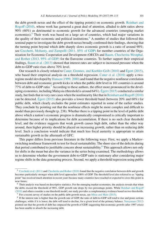
198 5 1990 1995 2000 2005 201 0

0.25

0.50

0.75

1.00Proba bil ities of Regime 1 [Low Deficit]

198 5 1990 1995 2000 2005 201 0

0.25

0.50

0.75

1.00Proba bil ities of Regime 2 [High Deficit]

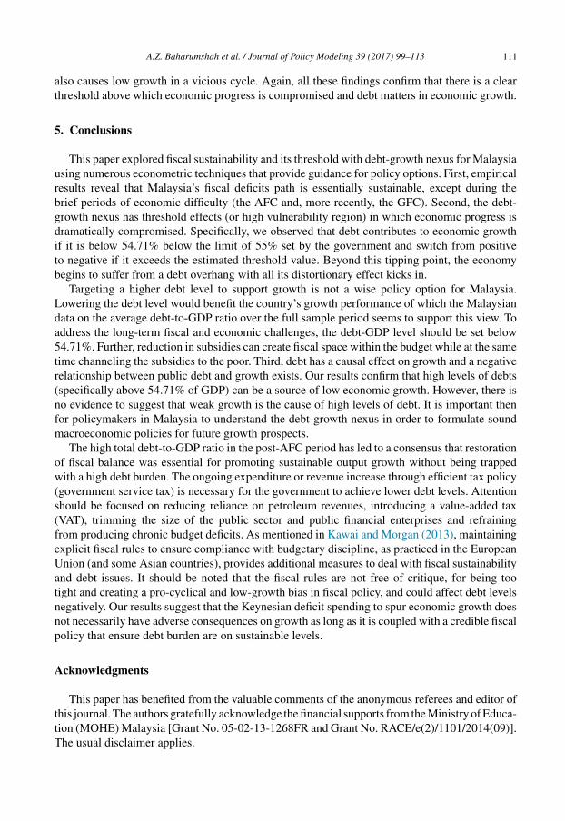
Fig. 2. Filtered and smoothed probabilities.

from a stable regime to an unstable one is higher than the probability of moving from an unstableregime to a stable one. The expected duration of the stable regime is estimated to be around 14.50quarters while that of the unstable regime is around 5.67 quarters. Clearly, the stable state is morelong lasting than the unstable one, as we expect that periods without recession or crisis tend tolast longer; an important guiding policy for Malaysia.

The explanation of this situation lies in the definition of the switching process. Countries mightsatisfy the solvency criterion but face important short-run imbalances, which may become largeenough to violate solvency in the future: when the long-run sustainability condition is satisfied,but the presence of temporary deviations from this condition create the danger that a countrymight be faced with debt problems in the future. This can also be seen from the duration of theregimes; if the duration of the unsustainable regime is longer than it is for the other regimes,it shows that the economy can remain on the unsustainable path without violating the solvencycondition. However, the longer the economy remains on that unsustainable path, the more likelyit is that it will end up with a balance of payments crisis.

We computed Fig. 2 using expectation maximization algorithm to present the filtered andsmoothed probabilities of being in a stable regime (low-deficit) and unstable regime (high-deficit).As expected, there is a clear tendency for the model to indicate a switch to an unstable regimeduring the economic downturns associated with the events of the commodity crisis in the late1980s, the AFC in 1997, the global economy slowdown in the early 2000s, and the recent GFC.From the viewpoint of policymakers and investors, it is comforting to know that the debt processis currently in a less volatile, stationary state. One must recall that the debt ratio dropped afterthe AFC but has increased slightly in the past few years. This insight is more than one gets from

108 A.Z. Baharumshah et al. / Journal of Policy Modeling 39 (2017) 99–113

Table 3Regime-switching error correction regressions.

Stable regime Unstable regime

Constant −0.018*** (0.006) 0.058*** (0.014)�Debtt−4 0.251*** (0.062) 0.448*** (0.111)�Debtt−8 0.288*** (0.048) 0.234* (0.128)�R-Gt−7 0.093 (0.077) 0.552*** (0.153)�R-Gt−8 0.347*** (0.080) 0.697*** (0.207)ECT t−1 −0.206* (0.118) 0.237*** (0.098)σ2 0.052*** (0.004) 0.058*** (0.006)DUM1989Q3 −0.253*** (0.019)DUM1991Q1 −0.703*** (0.048)DUM2008Q4 0.268*** (0.091)Diagnostic checkingLogL 162.173AIC −2.366Standard error 0.373Normality test (2) 0.271 [0.873]ARCH (4) 1.858 [0.124]Auto (12) 9.487 [0.661]Half-life estimated 0.3538HL (Q) 3.3695% CIs [1.15, 5.58]

Notes: ***, **, and * indicate significance at the 1%, 5%, and 10% levels, respectively. The values in square bracketsare probability values. Robust standard errors are in parentheses. σ2 refers to error variance. AIC is Akaike informa-tion criterion, and LogL is maximum log-likelihood. ARCH (m) is an mth order test for autoregressive conditionalheteroskedasticity. Auto(m) is an mth order for autocorrelation. d refers to the persistence parameter which computedfrom the error correction term (ECTt−1). HL(Q) is the half-life for the local-persistent model measured in quarters byln(0.5b(1))/(−1/nd ). The two-sided 95% confidence intervals (CIs) measured in quarterly were constructed according

to h0.50 ± 1.96se(λ)([− ln 0.5/λ][ln(λ)]−2

), where se(λ) = √2/(n(1/2)+(d/2)).

the unit-root tests showing whether the variable is stationary or nonstationary and illustrates themerits of a switching model toward policy making in Malaysia.

Table 3 shows the results for the regime-switching regression (MISAH-ECM). The modelpassed all the standard diagnostic tests. The impulse dummies are significant at the usual levels,indicating the presence of extreme values in the model. The equilibrium error correction term hasa negative sign and is significant at the indicated level in a low-deficit regime. We also observedthat the sign for the sum of the debt coefficients is positive. This verifies the long-run fiscalsustainability hypothesis, but in a low-deficit regime. To complement the analysis, we estimatethe speed of adjustment. The persistence parameter estimate is around 0.354 with a half-life pointestimate around 3.36 quarters, with the upper bound of the CIs of 5.58 quarters. Therefore, wecan conclude that rising debt ratios lead to a higher surplus, which has a tendency toward meanreversion. Implementing such a fiscal policy during a low-deficit regime should only be done withcaution.

4.1. Debt-growth nexus

To better understand the role of debt in an economy and when it becomes detrimental toeconomic growth, we apply the threshold regression model, as in Hansen (1999, 2000). We use

A.Z. Baharumshah et al. / Journal of Policy Modeling 39 (2017) 99–113 109

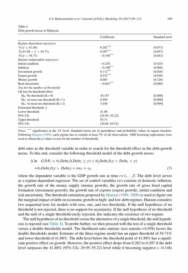
Table 4Debt-growth nexus in Malaysia.

Coefficient Standard error

Regime-dependent regressorsθ1(γ ≤ 41.88) 0.282*** (0.073)θ2(41.88 < γ < 54.71) 0.207*** (0.057)θ3(γ > 54.71) −0.146*** (0.043)Regime-independent regressorsInitial condition −0.230 (0.425)Inflation −0.108*** (0.009)Investment growth 0.112*** (0.028)Export growth 0.535*** (0.038)Money growth 0.083 (0.126)Real uncertainty −0.663*** (0.080)Test for the number of thresholdsLR test for threshold effect

H0: No threshold (K = 0) 10.157 [0.000]H0: At most one threshold (K = 1) 6.958 [0.000]H0: At most two threshold (K = 2) 3.450 [0.999]

Estimated threshold, γ

Lower threshold 41.8895% CIs [29.95, 55.22]Upper threshold 54.7195% CIs [30.85, 65.51]

Notes: *** significance at the 1% level. Standard errors are in parentheses and probability values in square brackets.Following Hansen (1999), each regime has to contain at least 5% of all observations. 1000 bootstrap replications wereused to obtain the p-values to test for the number of thresholds.

debt ratio as the threshold variable in order to search for the threshold effect in the debt-growthnexus. To this end, consider the following threshold model of the debt-growth nexus:

� ln GDPt = θ1DebttI(Debtt ≤ γ) + θ2DebttI(γ < Debtt < γ)

+θ3DebttI(γ > Debtt) + σwt + υt, (7)

where the dependent variable is the GDP growth rate at time t = 1,. . .,T. The debt level servesas a regime-dependent regressor. The set of control variables (w) consists of domestic inflation,the growth rate of the money supply (money growth), the growth rate of gross fixed capitalformation (investment growth), the growth rate of exports (export growth), initial condition andreal uncertainty. The threshold estimation proposed by Hansen (1999, 2000) is used to figure outthe marginal impact of debt on economic growth in high- and low-debt regimes. Hansen considerstwo sequential tests for models with zero, one, and two thresholds. If the null hypothesis of nothreshold is not rejected, there is no support for asymmetry. If the null hypothesis of no thresholdand the null of a single threshold easily rejected, this indicates the existence of two-regime.

The null hypothesis of no threshold versus the alternative of a single threshold, the null hypoth-esis is rejected (see Table 4). To probe further, we then proceed with the test of a single thresholdversus a double thresholds model. The likelihood ratio statistic (test statistic = 6.958) favors thedouble thresholds model. Estimate of the three-regime model has an upper threshold of 54.71%and lower threshold of 41.88%. The debt level below the threshold point of 41.88% has a signifi-cant positive effect on growth. However, the positive effect drops from 0.282 to 0.207 if the debtlevel surpasses the 41.88% (95% CIs: 29.95–55.22) level while it becoming negative (−0.146)

110 A.Z. Baharumshah et al. / Journal of Policy Modeling 39 (2017) 99–113

Table 5LA-VAR granger causality tests.

H0 k Economic growth / → debt Debt / → economic growth

Linear Model 4 4.174 (0.243) 7.507 (0.057)γ ≤ 41.88 3 4.898 (0.180) 8.380 (0.039)41.88 < γ < 54.71 7 3.231 (0.863) 9.304 (0.036)γ > 54.71 2 8.493 (0.014) 7.946 (0.019)

Notes: The null hypothesis H0: economic growth / → debt represents economic growth does not Granger-cause debt.Figures in ( ) refer to probability. k = optimum lag based on SIC. γ indicates the estimated debt threshold level.

if the threshold goes beyond 54.71%. In other words, debt has a simulative effect on growthbelow 54.71% and it found to hamper the health of the economy if it is higher than this level.By comparison, our estimated threshold level is close to the one provided by Caner et al. (2010)and Reinhart and Rogoff (2010). Focusing on the regime-dependent coefficients, investment andexports tended to promote economic growth, but inflation and real uncertainty have a negativeeffect on economic growth. The negative impact of real uncertainty on growth is supported byBaharumshah and Soon (2014). Finally, the model finds that financial depth did not play anyimportant role in economic growth in the sample period under review.

In sum, our empirical results have immediate implications for the government during periodsof high debt. High debt represents an extra cost of the policy, which has been ignored in mostempirical research. As argued in Cecchetti et al. (2011, p. 1), fiscal authorities “should also aimto keep debt well below the estimated thresholds so that even extraordinary events are unlike topush their debt to levels that become damaging to growth”. Debts can be beneficial as long as itis at modest levels, but beyond a certain tipping point, it becomes dangerous and excessive. Ourresults also echo the view in Spilimbergo, Symansky, Blanchard, and Cottarelli (2008) that theimpact of discretionary fiscal policy (like those adopted by the government after the GFC) onGDP is contingent on the level of debt. In particular, the positive impact on growth is larger whenlower debt levels are targeted. We find that the level of debt matters for fiscal policy effectivenessin Malaysia of which borrowing (debts) can be beneficial as long as it is at modest levels, butbeyond a certain tipping point, it becomes dangerous and excessive.

Although many papers have reported a negative correlation between debt and growth, wefind only a few (e.g., Jayaraman & Lau, 2009; Panizza & Presbitero, 2014; Gomez-Puig &Sosvilla-Rivero, 2015) that can make a case for causality between debt and economic growth.The causality issue is important in the present context: high debt may be the result of slug-gish growth. In other words, it is not obvious that indebtedness is the source of low economicgrowth. To this end, the lag augmented vector autoregressive (LA-VAR) approach of Toda andYamamoto (1995) suggested a unidirectional causality from debt to economic growth [ModifiedWald �2-statistics = 7.507; p-value = 0.057]. Table 5 presents the results for LA-VAR grangercausality tests. However, there is no evidence of causality from growth to debt [Modified Wald�2-statistics = 4.174; p-value = 0.243]. For robust check, we take the analysis further by splittingour sample into two—one to present debts level below 54.71% and others to present the periodwhere debt levels exceed 54.71%. Two points are noted from the causality test. First, the uni-directional causality mentioned earlier is found to hold if the debt is below 54.71. Second, weuntangle feedback causality between debt and growth when the debt is above the 54.71 thresholdlevel. Tax revenues and government expenditure tend to be functions of economic growth, andgrowth has the potential to reduce the deficit/GDP and debt/GDP ratios as well. But high debt

A.Z. Baharumshah et al. / Journal of Policy Modeling 39 (2017) 99–113 111

also causes low growth in a vicious cycle. Again, all these findings confirm that there is a clearthreshold above which economic progress is compromised and debt matters in economic growth.

5. Conclusions

This paper explored fiscal sustainability and its threshold with debt-growth nexus for Malaysiausing numerous econometric techniques that provide guidance for policy options. First, empiricalresults reveal that Malaysia’s fiscal deficits path is essentially sustainable, except during thebrief periods of economic difficulty (the AFC and, more recently, the GFC). Second, the debt-growth nexus has threshold effects (or high vulnerability region) in which economic progress isdramatically compromised. Specifically, we observed that debt contributes to economic growthif it is below 54.71% below the limit of 55% set by the government and switch from positiveto negative if it exceeds the estimated threshold value. Beyond this tipping point, the economybegins to suffer from a debt overhang with all its distortionary effect kicks in.

Targeting a higher debt level to support growth is not a wise policy option for Malaysia.Lowering the debt level would benefit the country’s growth performance of which the Malaysiandata on the average debt-to-GDP ratio over the full sample period seems to support this view. Toaddress the long-term fiscal and economic challenges, the debt-GDP level should be set below54.71%. Further, reduction in subsidies can create fiscal space within the budget while at the sametime channeling the subsidies to the poor. Third, debt has a causal effect on growth and a negativerelationship between public debt and growth exists. Our results confirm that high levels of debts(specifically above 54.71% of GDP) can be a source of low economic growth. However, there isno evidence to suggest that weak growth is the cause of high levels of debt. It is important thenfor policymakers in Malaysia to understand the debt-growth nexus in order to formulate soundmacroeconomic policies for future growth prospects.

The high total debt-to-GDP ratio in the post-AFC period has led to a consensus that restorationof fiscal balance was essential for promoting sustainable output growth without being trappedwith a high debt burden. The ongoing expenditure or revenue increase through efficient tax policy(government service tax) is necessary for the government to achieve lower debt levels. Attentionshould be focused on reducing reliance on petroleum revenues, introducing a value-added tax(VAT), trimming the size of the public sector and public financial enterprises and refrainingfrom producing chronic budget deficits. As mentioned in Kawai and Morgan (2013), maintainingexplicit fiscal rules to ensure compliance with budgetary discipline, as practiced in the EuropeanUnion (and some Asian countries), provides additional measures to deal with fiscal sustainabilityand debt issues. It should be noted that the fiscal rules are not free of critique, for being tootight and creating a pro-cyclical and low-growth bias in fiscal policy, and could affect debt levelsnegatively. Our results suggest that the Keynesian deficit spending to spur economic growth doesnot necessarily have adverse consequences on growth as long as it is coupled with a credible fiscalpolicy that ensure debt burden are on sustainable levels.

Acknowledgments

This paper has benefited from the valuable comments of the anonymous referees and editor ofthis journal. The authors gratefully acknowledge the financial supports from the Ministry of Educa-tion (MOHE) Malaysia [Grant No. 05-02-13-1268FR and Grant No. RACE/e(2)/1101/2014(09)].The usual disclaimer applies.

112 A.Z. Baharumshah et al. / Journal of Policy Modeling 39 (2017) 99–113

References

Ahmed, S., & Rogers, J. H. (1995). Government budget deficits and trade deficits: Are present value constraints satisfiedin long-term data? Journal of Monetary Economics, 36(2), 351–374.

Baharumshah, A. Z., & Lau, E. (2007). Regime changes and the sustainability of fiscal imbalance in East Asian countries.Economic Modelling, 24(6), 878–894.

Baharumshah, A. Z., & Soon, S. V. (2014). Inflation, inflation uncertainty and output growth: What does the data say forMalaysia? Journal of Economic Studies, 41(3), 370–386.

Baum, A., Checherita-Westphal, C., & Rother, P. (2013). Debt and growth: New evidence for the euro area. Journal ofInternational Money and Finance, 32(February), 809–821.

Bohn, H. (2007). Are stationarity and cointegration restrictions really necessary for the intertemporal budget constraint?Journal of Monetary Economics, 54(7), 1837–1847.

Byrne, J., Fiess, N., & MacDonald, R. (2011). The global dimension to fiscal sustainability. Journal of Macroeconomics,33(2), 137–150.

Caner, M., Grennes, T., & Koehler-Geib, F. (2010). Finding the tipping point: When sovereign debt turns bad. WorldBank Policy Research Working Paper No. 5391.

Cecchetti, S. G., Mohanty, M. S., & Zampolli, F. (2011). The real effects of debt. Bank for International Settlements (BIS)Working Papers No. 352.

Checherita, C., & Rother, P. (2010). The impact of high and growing government debt on economic growth: An empiricalinvestigation for the euro area. European Central Bank Working Paper Series No. 1237.

Chen, S.-W. (2014). Testing for fiscal sustainability: New evidence from the G-7 and some European countries. EconomicModelling, 37(February), 1–15.

Davies, R. B. (1987). Hypothesis testing when a nuisance parameter is present only under the alternatives. Biometrika,74(1), 33–43.

DeLong, J. B., & Summers, L. H. (2012). Fiscal policy in a depressed economy. The Brookings Papers on EconomicActivity, 44(1), 233–297.

Dogan, I., & Bilgili, F. (2014). The non-linear impact of high and growing government external debt on economic growth:A Markov regime-switching approach. Economic Modelling, 39(April), 213–220.

Égert, B. (2015). Public debt, economic growth and nonlinear effect: Myth or reality? Journal of Macroeconomics,43(March), 226–238.

Gomez-Puig, M., & Sosvilla-Rivero, S. (2015). The causal relationship between debt and growth in EMU countries.Journal of Policy Modeling, 37(6), 974–989.

Hamilton, J. D. (1989). A new approach to the economic analysis of nonstationary time series and the business cycle.Econometrica, 57(2), 357–384.

Hamilton, J. D. (1990). Analysis of time series subject to changes in regime. Journal of Econometrics, 45(1–2), 39–70.Hamilton, J. D., & Flavin, M. A. (1986). On the limitations of government borrowing: A framework for empirical testing.

The American Economic Review, 76(4), 808–819.Hansen, B. E. (1999). Threshold effects in non-dynamic panels: Estimation, testing, and inference. Journal of Economet-

rics, 93(2), 345–368.Hansen, B. E. (2000). Sample splitting and threshold estimation. Econometrica, 68(3), 575–603.Holmes, M. J., Otero, J., & Panagiotidis, T. (2010). Are EU budget deficits stationary? Empirical Economics, 38(3),

767–778.Jayaraman, T. K., & Lau, E. (2009). Does external debt lead to economic growth in Pacific Island countries. Journal of

Policy Modeling, 31(2), 272–288.Kawai, M., & Morgan, P. J. (2013). Long-term issues for fiscal sustainability in emerging Asia. Public Policy Review,

9(4), 751–770.Kim, C.-J. (1994). Dynamic linear models with Markov-switching. Journal of Econometrics, 60(1–2), 1–22.Kim, S., & Lima, L. R. (2010). Local persistence and the PPP hypothesis. Journal of International Money and Finance,

29(3), 555–569.Lawrence, C. T., & Tits, A. L. (2001). A computationally efficient feasible sequential quadratic programming algorithm.

SIAM Journal on Optimization, 11(4), 1092–1118.Mahdavi, S., & Westerlund, J. (2011). Fiscal stringency and fiscal sustainability: Panel evidence from the American state

and local governments. Journal of Policy Modeling, 33(6), 953–969.Mitze, T., & Matz, F. (2015). Public debt and growth in German federal states: What can Europe learn? Journal of Policy

Modeling, 37(2), 208–228.

A.Z. Baharumshah et al. / Journal of Policy Modeling 39 (2017) 99–113 113

Narayanan, S. (2012). Public sector resource management. In H. Hill, S. Y. Tham, & H. M. Z. Ragayah (Eds.), Malaysia’sdevelopment challenges: Graduating from the middle (pp. 131–154). London: Rouledge.

Panizza, U., & Presbitero, A. F. (2014). Public debt and economic growth: Is there a causal effect? Journal of Macroeco-nomics, 41(C), 21–41.

Pattillo, C., Poirson, H., & Ricci, L. (2002). External debt and growth. International Monetary Fund Working Paper No.WP/02/69.

Phillips, P. C. B., Moon, H. R., & Xiao, Z. (2001). How to estimate autoregressive roots near unity. Econometric Theory,17(1), 29–69.

Quintos, C. E. (1995). Sustainability of the deficit process with structural shifts. Journal of Business and EconomicStatistics, 13(4), 409–417.

Raybaudi, M., Sola, M., & Spagnolo, F. (2004). Red signals: Current account deficits and sustainability. EconomicsLetters, 84(2), 217–223.

Reinhart, C. M., & Rogoff, K. S. (2010). Growth in a time of debt. American Economic Review, 100(2), 573–578.Rossi, B. (2005). Confidence intervals for half-life deviations from purchasing power parity. Journal of Business &

Economic Statistics, 23(4), 432–442.Spilimbergo, A., Symansky, S., Blanchard, O., & Cottarelli, C. (2008). Fiscal policy for the crisis. International Monetary

Fund (IMF) Staff Position Note, No. SPN/08/01, 1–37.Toda, H. Y., & Yamamoto, T. (1995). Statistical inference in vector autoregressions with possibly integrated processes.

Journal of Econometrics, 66(1–2), 225–250.Wagner, G. A., & Elder, E. M. (2005). The role of budget stabilization funds in smoothing government expenditures over

the business cycle. Public Finance Review, 33(4), 439–465.