Contents lists available at ScienceDirect

Journal of Economic Dynamics & Control

Journal of Economic Dynamics & Control 37 (2013) 2582–2601

0165-18http://d

n CorrE-m1 Th

events (

journal homepage: www.elsevier.com/locate/jedc

Fiscal news and macroeconomic volatility

Benjamin Born a,n, Alexandra Peter b, Johannes Pfeifer c

a University of Mannheim, L7, 3-5, 68131 Mannheim, Germanyb International Monetary Fund, 700 19th Street, NW, Washington, DC 20431, USAc University of Tuebingen, Mohlstr. 36, 72074 Tuebingen, Germany

a r t i c l e i n f o

Article history:Received 12 October 2011Received in revised form29 March 2013Accepted 24 June 2013Available online 1 July 2013

JEL classification:E32E62C11

Keywords:Anticipated tax shocksSources of aggregate fluctuationsBayesian estimation

89/$ - see front matter & 2013 Elsevier B.V.x.doi.org/10.1016/j.jedc.2013.06.011

esponding author.ail addresses: born@uni-mannheim.de (B. Boere is a prominent literature branch dealingPoterba, 1988; Parker, 1999; House and Shap

a b s t r a c t

This paper analyzes the contribution of anticipated capital and labor tax shocks tobusiness cycle volatility in an estimated New Keynesian business cycle model. While fiscalpolicy accounts for about 15% of output variance at business cycle frequencies, this mostlyderives from anticipated government spending shocks. Tax shocks, both anticipated andunanticipated, contribute little to the fluctuations of real variables. However, anticipatedcapital tax shocks do explain a sizable part of inflation fluctuations, accounting for up to12% of its variance. In line with earlier studies, news shocks in total account for about 50%of output variance. Further decomposing this news effect, we find permanent total factorproductivity news shocks to be most important. When looking at the federal level insteadof total government, the importance of anticipated tax and spending shocks significantlyincreases, suggesting that fiscal policy at the subnational level typically counteracts theeffects of federal fiscal policy shocks.

& 2013 Elsevier B.V. All rights reserved.

1. Introduction

The current paper analyzes the role of news about future fiscal policy (“fiscal news”), and in particular the anticipation oftax rate changes, for business cycle fluctuations. Recent macroeconomic research has increasingly shifted from explainingbusiness cycle fluctuations through contemporaneous shocks to explaining them by anticipated, or news, shocks. Rationalagents, anticipating future changes will already react today to these news (see, e.g., Beaudry and Portier, 2004, 2006;Jaimovich and Rebelo, 2009; Schmitt-Grohé and Uribe, 2012). However, most empirical studies on the effects of anticipatedshocks on business cycles have focused on news about future productivity (see, e.g., Fujiwara et al., 2011; Khan andTsoukalas, 2012; Forni et al., 2011).1

This is remarkable for two reasons. First, fiscal measures are usually publicly debated well in advance and often knownbefore becoming effective, i.e., there are considerable decision and implementation lags. A tax bill typically takes about oneyear from the U.S. President's initial proposal to the law's enactment and another year until the tax change becomes effective(Yang, 2005; Mertens and Ravn, 2011). As a recent example, consider the Patient Protection and Affordable Care Act(“Obamacare”), whose core contents were debated for almost one year and whose financing provisions will only phase ingradually over time. Second, surprise fiscal policy shocks have long been discussed as a potential prominent driver of the

All rights reserved.

rn), apeter@imf.org (A. Peter), johannes.pfeifer@uni-tuebingen.de (J. Pfeifer).with the importance of fiscal foresight. However, its focus has mostly been on analyzing single taxiro, 2006) or tracing out the consequences for econometric analyses (Yang, 2005; Leeper et al., 2013).

B. Born et al. / Journal of Economic Dynamics & Control 37 (2013) 2582–2601 2583

business cycle (see e.g. Baxter and King, 1993; McGrattan, 1994; Jones, 2002; Cardia et al., 2003). McGrattan (1994) forexample attributes one third of the U.S. business cycle variance to distortionary taxation, while McGrattan (2012) arguesthat changes in business taxation can explain one third of the output drop during the Great Depression.2 This potentialimportance of fiscal policy shocks, combined with the fact that many fiscal policy measures are known well in advance,makes fiscal news a natural candidate for explaining aggregate fluctuations.

We add upon the previous literature by explicitly analyzing the business cycle variance contribution of fiscal news. Forthis purpose, we employ a New Keynesian Dynamic Stochastic General Equilibrium (DSGE) business cycle model featuringseveral real and nominal rigidities as well as various shocks identified as important drivers of the business cycle. Weaugment the model with a government sector featuring distortionary labor and capital taxes that follow fiscal rules withendogenous feedback to debt and current economic conditions. Our main focus lies on the effects of fiscal news, but we alsocontrol for anticipation in total factor productivity (TFP), investment-specific productivity, and the wage markup. The modelis estimated by full information (Bayesian) methods using quarterly U.S. data from 1955 to 2006. Model-based estimationallows us to circumvent the issue of non-invertibility that can arise when estimating structural vector autoregressions(VARs) in the presence of anticipation effects (Leeper et al., 2013; Fernández-Villaverde et al., 2007; Hansen and Sargent,1991).3

Computing forecast error variance decompositions, we find that for the U.S. total government fiscal foresight plays only amoderate role in explaining business cycles. With an unconditional variance share of 13% anticipated government spendingshocks are the fiscal variable with the largest effect on output variance. In contrast, contemporaneous and anticipated laborand capital tax shocks are not important drivers of business cycles, together contributing only 2% to output fluctuations.Tax shocks, and particularly anticipated tax shocks, are only relevant for explaining the variance of inflation. Depending onthe forecast horizon, anticipated capital tax shocks contribute 8% to 12% to its variance. Surprise capital tax shocks areresponsible for another 4%. In contrast, the effects of labor tax shocks are negligible. Overall, these results are in line with theVAR evidence of Forni and Gambetti (2010) that 16% of output fluctuations are due to anticipated government spendingshocks and the finding of Forni et al. (2009) for the EU that unanticipated tax shocks are a negligible factor for explainingbusiness cycles. Also in line with previous studies considering either only surprise shocks (e.g. Smets and Wouters, 2007) oralso news shocks (e.g. Schmitt-Grohé and Uribe, 2012), we find that technology shocks are an important driver of outputfluctuations.

In our estimated model news shocks explain about 50% of the variance of output, with the main effect coming from newsabout TFP. This result conforms well with VAR evidence by Barsky and Sims (2011) and Kurmann and Otrok (forthcoming),who both find a similar fraction of output fluctuations explained by anticipated shocks.

The two papers most closely related to ours are recent contributions by Mertens and Ravn (2012) and Schmitt-Grohé andUribe (2012). Mertens and Ravn (2012) use a VAR to analyze the business cycle contribution of narratively identifiedanticipated and unanticipated tax shocks.4 They find that both types of tax shocks together explain 20% to 25% of outputvariance, with anticipation accounting for the majority. The difference in our findings to Mertens and Ravn (2012) can beexplained by the fact that their study focuses on legislated federal fiscal measures. Whenwe estimate our baseline model onfederal government data only, we find that fiscal foresight accounts for 37% of the unconditional output variance, withanticipated tax shocks being responsible for 15%. Moreover, Mertens and Ravn (2012) find that an anticipated tax cutgenerates a recession during the anticipation phase before the realization of the tax cut. Our baseline model estimated withtotal government data does not generate such an anticipatory recession, while the model estimated on federal governmentdoes. Those differences in results for using total vs. federal government data suggests that reactions at the subnational levelsof government tend to counteract federal fiscal measures. Thus, considering the entire fiscal sector instead of the federalgovernment only delivers a more representative picture of the average response to a fiscal shock as it does not rely onkeeping the expenditures and revenues at the subnational level constant—something that seems not to happen in practice.

Schmitt-Grohé and Uribe (2012) evaluate the role of news about TFP, investment-specific technology, wage markup, andgovernment spending shocks in an estimated RBC model with various real rigidities. In their setup, news shocks account for41% of output fluctuations. But while they find government spending shocks to explain 10% of output variance, evenlydistributed across surprise, one and two year anticipated shocks, they do not consider foresight about the financing side ofthe government budget constraint and do not allow for fiscal rules that contain endogenous feedback.

Our paper is also related to other DSGE-based papers focusing on the effects of anticipated technology shocks. Davis(2007), using a New Keynesian model, estimates news shocks to be responsible for 50% of output fluctuations. Fujiwara et al.(2011) extend the New Keynesian models of Smets and Wouters (2007) and Christiano et al. (2005) to include news about

2 Although Forni et al. (2009) find that unanticipated tax shocks contribute little to macroeconomic fluctuations of the Euro area, this could in principlebe the result of ignoring fiscal foresight.

3 Non-invertibility means that the DGSE-model has a VARMA representation that cannot be inverted to yield a finite-order VAR in the observables.Hence, the true innovations do not perfectly map into the VAR residuals. Non-invertibility arises, e.g., when the information set of an econometrician issmaller than that of the forward-looking agents. It is important to note that this does not mean that VARs cannot be used to estimate news shocks at all.Sims (2012), for example, shows that in some cases it may be possible to recover the shocks using a structural VAR. By including enough lags and forward-looking variables, it may be possible to move the non-invertible root(s) close enough to unity so that the discrepancy between true structural errors andthe estimated ones becomes small (see also Giannone and Reichlin, 2006; Forni et al., 2011; Gambetti, 2012).

4 Mertens and Ravn (2012) classify Romer and Romer (2010) tax shocks according to the time passed between the presidential signing of a bill and thetax changes becoming effective into anticipated and contemporaneous shocks.

B. Born et al. / Journal of Economic Dynamics & Control 37 (2013) 2582–26012584

TFP. They estimate news shocks to explain 9% of the unconditional output variance. The paper of Khan and Tsoukalas (2012)uses the same basic New Keynesian model framework, but additionally allows for news about investment-specifictechnology growth. In their estimated model, both types of news shocks together account for less than 10%.

The outline of the paper is the following. Section 2 introduces the DSGE model with fiscal foresight, while Section 3presents the estimation approach and results. In Section 4, we compute variance decompositions and impulse responsesand consider the distinction between total and federal government. Section 5 concludes.

2. A DSGE model with fiscal foresight

We use a medium-scale DSGE model featuring various real and nominal frictions as well as a variety of shocks that havebeen identified as important drivers of the business cycle (see, e.g., Smets and Wouters, 2007; Justiniano et al., 2010a). Weincorporate both contemporaneous and anticipated elements into the shock processes as in Schmitt-Grohé and Uribe (2012)and allow for non-stationary shocks. We first discuss the information structure of the shock processes in the next subsectionbefore describing the model in detail.

2.1. Shock structure

Our model features 10 sources of stochastic fluctuations. On the government side, we include shocks to labor and capitaltax rates τnt and τkt , a shock to government spending gt , and a monetary policy shock ξRt . The technology shocks consideredare shocks to stationary neutral productivity zt , non-stationary productivity Xt , stationary investment-specific productivityzIt , and non-stationary investment-specific productivity At . In addition, the model includes a preference shock ξpreft and awage markup shock μwt .

The monetary policy shock and the preference shock are assumed to only contain a contemporaneous, unanticipatedcomponent. For the other shocks, we follow the framework proposed by Schmitt-Grohé and Uribe (2012) and allow for bothcontemporaneous shocks and shocks that are anticipated 4 and 8 periods in advance. Anticipation horizons of 4 and 8quarters fulfill the aim of capturing longer anticipation horizons while keeping the state space at a manageable level. This iscrucial as each additional anticipation horizon is an additional state variable. While specifically choosing 4 and 8 quarters ofanticipation might be seen as arbitrary, this assumption can be rationalized by the workings of the political system. Fourquarters of anticipation are close to the average length of a tax bill from the President's proposal announcement toenactment (Yang, 2005). Eight quarters serve as a plausible upper bound for the anticipation of shocks to tax rates asCongressional elections take place every two years. We think this makes it very unlikely that people are able to correctlypredict both the reigning majority and the tax laws being implemented by the next Congress. The same, of course, applies tospending bills. For reasons of symmetry, we then assume this anticipation structure for all shock processes, except forpreferences and monetary policy, where a structural interpretation of anticipated shocks would be tenuous.

The general structure for shock ϵi; i∈fτn; τk; g; z; x; zI; a;wg is given by

ϵi ¼ ε0i;t þ ε4i;t�4 þ ε8i;t�8; ð1Þ

where εji;t�j; j∈f0;4;8g denotes a shock to variable i that becomes known in period t�j and hits the economy j periods later.

For example, ε4τn;t�4 denotes a four period anticipated shock to the labor tax rate that becomes known at time t�4 and

becomes effective at time t. The shocks are assumed to have mean 0, standard deviation sji, to be serially uncorrelated, and

to be uncorrelated across anticipation horizons, i.e. Eðεji;t�jÞ ¼ 0 and Eðεki;tεli;t�jÞ ¼ ðski Þ2 for j¼ 0; k¼ l, and 0 otherwise.

Moreover, they are uncorrelated across shock types im; in∈i, Eðεkim ;tεlin ;t�jÞ ¼ 0 ∀j; k; l and im≠in. The only exception is that we

allow for contemporaneous correlation between the labor and capital tax rate shocks at all anticipation horizons, i.e.

Eðεjτk;t�jεjτn;t�jÞ ¼ sjτk;τn. This assumption is due to the fact that in the construction of tax rates one part of proprietor's income

is attributed to capital taxation and the other part is attributed to labor taxation. Moreover, many tax measures affect boththe capital and the labor margin.

The assumed information structure implies that agents foresee future shocks to the extent of already known but not yetrealized shocks εmi;t�j; m4 j. The forward-looking behavior of rational optimizing agents leads them to react to anticipated

shocks even before they are realized. By imposing a structural model on the data, this anticipatory behavior enables theeconometrician to achieve identification.

2.2. Conceptualizing tax shocks

The tax shocks considered in the present work do not necessarily stem from actual changes in the labor and capital taxrates. Rather, they are interpreted as the probability weighted effect of tax actions under legislative debate or due tojudicative decisions. They are the product of the likelihood of a tax change and of the size of this effect, as perceived byrational agents forming expectations about the future path of taxes. Hence, our definition is wider than the one consideredby Mertens and Ravn (2012), who restrict their attention to the shocks directly deriving from the legislative process. Shocks

B. Born et al. / Journal of Economic Dynamics & Control 37 (2013) 2582–2601 2585

deriving, e.g., from the SEC suing against the legality of a tax shelter would be excluded from their definition but not fromours.5 Note that news shocks are distinct from pure uncertainty about future taxes. While the former are associated with ananticipated change in the mean of the tax rate, tax uncertainty shocks can be conceptualized as mean-preserving spreads.6

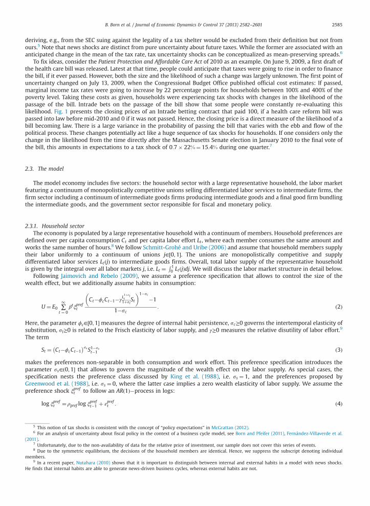
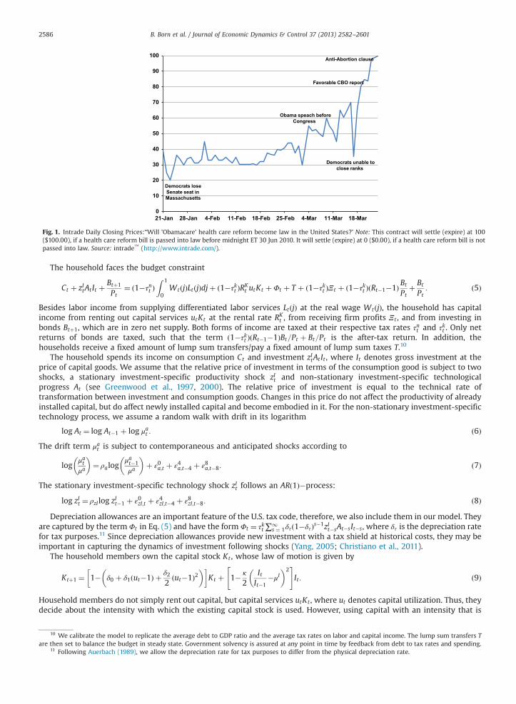
To fix ideas, consider the Patient Protection and Affordable Care Act of 2010 as an example. On June 9, 2009, a first draft ofthe health care bill was released. Latest at that time, people could anticipate that taxes were going to rise in order to financethe bill, if it ever passed. However, both the size and the likelihood of such a change was largely unknown. The first point ofuncertainty changed on July 13, 2009, when the Congressional Budget Office published official cost estimates: If passed,marginal income tax rates were going to increase by 22 percentage points for households between 100% and 400% of thepoverty level. Taking these costs as given, households were experiencing tax shocks with changes in the likelihood of thepassage of the bill. Intrade bets on the passage of the bill show that some people were constantly re-evaluating thislikelihood. Fig. 1 presents the closing prices of an Intrade betting contract that paid 100, if a health care reform bill waspassed into law before mid-2010 and 0 if it was not passed. Hence, the closing price is a direct measure of the likelihood of abill becoming law. There is a large variance in the probability of passing the bill that varies with the ebb and flow of thepolitical process. These changes potentially act like a huge sequence of tax shocks for households. If one considers only thechange in the likelihood from the time directly after the Massachusetts Senate election in January 2010 to the final vote ofthe bill, this amounts in expectations to a tax shock of 0:7� 22%¼ 15:4% during one quarter.7

2.3. The model

The model economy includes five sectors: the household sector with a large representative household, the labor marketfeaturing a continuum of monopolistically competitive unions selling differentiated labor services to intermediate firms, thefirm sector including a continuum of intermediate goods firms producing intermediate goods and a final good firm bundlingthe intermediate goods, and the government sector responsible for fiscal and monetary policy.

2.3.1. Household sectorThe economy is populated by a large representative household with a continuum of members. Household preferences are

defined over per capita consumption Ct and per capita labor effort Lt , where each member consumes the same amount andworks the same number of hours.8 We follow Schmitt-Grohé and Uribe (2006) and assume that household members supplytheir labor uniformly to a continuum of unions j∈½0;1�. The unions are monopolistically competitive and supplydifferentiated labor services LtðjÞ to intermediate goods firms. Overall, total labor supply of the representative householdis given by the integral over all labor markets j, i.e. Lt ¼

R 10 LtðjÞdj. We will discuss the labor market structure in detail below.

Following Jaimovich and Rebelo (2009), we assume a preference specification that allows to control the size of thewealth effect, but we additionally assume habits in consumption:

U ¼ E0 ∑1

t ¼ 0βtξpreft

Ct�ϕcCt�1�γL1þslt1þsl

St

� �1�sc

�1

1�sc: ð2Þ

Here, the parameter ϕc∈½0;1� measures the degree of internal habit persistence, sc≥0 governs the intertemporal elasticity ofsubstitution, sl≥0 is related to the Frisch elasticity of labor supply, and γ≥0 measures the relative disutility of labor effort.9

The term

St ¼ Ct�ϕcCt�1� �ss S1�ss

t�1 ð3Þ

makes the preferences non-separable in both consumption and work effort. This preference specification introduces theparameter ss∈ð0;1� that allows to govern the magnitude of the wealth effect on the labor supply. As special cases, thespecification nests the preference class discussed by King et al. (1988), i.e. ss ¼ 1, and the preferences proposed byGreenwood et al. (1988), i.e. ss ¼ 0, where the latter case implies a zero wealth elasticity of labor supply. We assume thepreference shock ξpreft to follow an ARð1Þ�process in logs:

log ξpreft ¼ ρpref log ξpreft�1 þ εpreft : ð4Þ

5 This notion of tax shocks is consistent with the concept of “policy expectations” in McGrattan (2012).6 For an analysis of uncertainty about fiscal policy in the context of a business cycle model, see Born and Pfeifer (2011), Fernández-Villaverde et al.

(2011).7 Unfortunately, due to the non-availability of data for the relative price of investment, our sample does not cover this series of events.8 Due to the symmetric equilibrium, the decisions of the household members are identical. Hence, we suppress the subscript denoting individual

members.9 In a recent paper, Nutahara (2010) shows that it is important to distinguish between internal and external habits in a model with news shocks.

He finds that internal habits are able to generate news-driven business cycles, whereas external habits are not.

Democrats lose Senate seat in Massachusetts

Obama speach before Congress

Democrats unable to close ranks

Favorable CBO report

Anti-Abortion clause

0

10

20

30

40

50

60

70

80

90

100

21-Jan 28-Jan 4-Feb 11-Feb 18-Feb 25-Feb 4-Mar 11-Mar 18-Mar

Fig. 1. Intrade Daily Closing Prices:“Will ’Obamacare’ health care reform become law in the United States?’ Note: This contract will settle (expire) at 100($100.00), if a health care reform bill is passed into law before midnight ET 30 Jun 2010. It will settle (expire) at 0 ($0.00), if a health care reform bill is notpassed into law. Source: intrade™ (http://www.intrade.com/).

B. Born et al. / Journal of Economic Dynamics & Control 37 (2013) 2582–26012586

The household faces the budget constraint

Ct þ zItAtIt þ Btþ1

Pt¼ ð1�τnt Þ

Z 1

0WtðjÞLtðjÞdjþ ð1�τkt ÞRK

t utKt þΦt þ T þ ð1�τkt ÞΞt þ ð1�τkt ÞðRt�1�1ÞBt

Ptþ Bt

Pt: ð5Þ

Besides labor income from supplying differentiated labor services LtðjÞ at the real wage WtðjÞ, the household has capitalincome from renting out capital services utKt at the rental rate RK

t , from receiving firm profits Ξt , and from investing inbonds Btþ1, which are in zero net supply. Both forms of income are taxed at their respective tax rates τnt and τkt . Only netreturns of bonds are taxed, such that the term ð1�τkt ÞðRt�1�1ÞBt=Pt þ Bt=Pt is the after-tax return. In addition, thehouseholds receive a fixed amount of lump sum transfers/pay a fixed amount of lump sum taxes T.10

The household spends its income on consumption Ct and investment zItAt It , where It denotes gross investment at theprice of capital goods. We assume that the relative price of investment in terms of the consumption good is subject to twoshocks, a stationary investment-specific productivity shock zIt and non-stationary investment-specific technologicalprogress At (see Greenwood et al., 1997, 2000). The relative price of investment is equal to the technical rate oftransformation between investment and consumption goods. Changes in this price do not affect the productivity of alreadyinstalled capital, but do affect newly installed capital and become embodied in it. For the non-stationary investment-specifictechnology process, we assume a random walk with drift in its logarithm

log At ¼ log At�1 þ log μat : ð6ÞThe drift term μat is subject to contemporaneous and anticipated shocks according to

logμatμa

� �¼ ρalog

μat�1μa

� �þ ε0a;t þ ε4a;t�4 þ ε8a;t�8: ð7Þ

The stationary investment-specific technology shock zIt follows an ARð1Þ�process:

log zIt ¼ ρzIlog zIt�1 þ ε0zI;t þ ε4zI;t�4 þ ε8zI;t�8: ð8Þ

Depreciation allowances are an important feature of the U.S. tax code, therefore, we also include them in our model. Theyare captured by the term Φt in Eq. (5) and have the form Φt ¼ τkt∑

1s ¼ 1δτð1�δτÞs�1zIt�sAt�sIt�s, where δτ is the depreciation rate

for tax purposes.11 Since depreciation allowances provide new investment with a tax shield at historical costs, they may beimportant in capturing the dynamics of investment following shocks (Yang, 2005; Christiano et al., 2011).

The household members own the capital stock Kt , whose law of motion is given by

Ktþ1 ¼ 1� δ0 þ δ1ðut�1Þ þ δ22ðut�1Þ2

� �� �Kt þ 1� κ

2ItIt�1

�μI� �2

" #It : ð9Þ

Household members do not simply rent out capital, but capital services utKt , where ut denotes capital utilization. Thus, theydecide about the intensity with which the existing capital stock is used. However, using capital with an intensity that is

10 We calibrate the model to replicate the average debt to GDP ratio and the average tax rates on labor and capital income. The lump sum transfers Tare then set to balance the budget in steady state. Government solvency is assured at any point in time by feedback from debt to tax rates and spending.

11 Following Auerbach (1989), we allow the depreciation rate for tax purposes to differ from the physical depreciation rate.

B. Born et al. / Journal of Economic Dynamics & Control 37 (2013) 2582–2601 2587

higher than normal is not costless, but leads to higher depreciation of the capital stock. This is captured by the increasingand convex function δðutÞ ¼ δ0 þ δ1ðut�1Þ þ δ2=2ðut�1Þ2, with δ0; δ1; δ240. Without loss of generality, capital utilization insteady state is normalized to 1. Following Christiano et al. (2005), we assume the presence of investment adjustment costsSðIt=It�1Þ ¼ κ=2ðIt=It�1�μIÞ2 to dampen the volatility of investment over the business cycle. κ40 is a parameter governingthe curvature of the investment adjustment costs and μI is the steady state growth rate of investment, which is equal to thesteady state growth rate of capital. This specification assures that the investment adjustment costs are minimized and equalto 0 along the balanced growth path, i.e. S¼ S′¼ 0 and S″40, where the primes denote derivatives.

The household maximizes its utility, Eq. (2), by choosing Ct ; Lt ; St ; Btþ1; Ktþ1; ut , and It , subject to the budget constraint (5),the law of motion for capital (9), and the resource constraint for aggregate labor given by (10) below.

2.3.2. Labor marketThe labor market is characterized by differentiated labor services and staggered wage setting. To model these features

without letting idiosyncratic wage risk affect the household members, and thus making aggregation intractable, we assumea continuum of unions j; j∈½0;1�. The household members supply their labor LtðjÞ equally to the unions, which aremonopolistically competitive and supply differentiated labor LtðjÞ to intermediate firms at wage WtðjÞ. Every period, a unionj is able to re-optimize its wage with probability ð1�θwÞ, 0oθwo1. A union j that is not able to re-optimize indexes itsnominal wage to the price level according to WtðjÞPt ¼ ðΠt�1ÞχwΠ1�χwμytWt�1ðjÞPt�1, where the parameter χw∈½0;1� measuresthe degree of indexing, Π is steady state gross inflation, and μyt is the gross growth rate of output (see, e.g., Smets andWouters, 2003). Thus, in the absence of price adjustment the wage still partly adapts to changes in productivity and inflation(Christiano et al., 2008), thereby assuring that no current wage contract will deviate arbitrarily far from the currentoptimal wage.

Household members supply the amount of labor services that is demanded at the current wage. Unions that can resettheir wages choose the real wage that maximizes the expected utility of its members, taking into account the demand for itslabor services LtðjÞ ¼ ðWtðjÞ=WtÞ�ηw;t Lcomp

t , where Lcompt is the aggregate demand for composite labor services, the respective

resource constraint

Lt ¼ Lcompt

Z 1

0

WtðjÞWt

� ��ηw;t

dj ; ð10Þ

and the aggregate wage level Wt ¼ ðR 10 WtðjÞ1�ηw;t djÞ1=ð1�ηw;t Þ. The time-varying substitution elasticity ηw;t allows us to includea wage markup shock μwt ¼ ðηw;t�1Þ�1 that follows:

logμwtμw

� �¼ ρw log

μwt�1μw

� �þ ε0w;t þ ε4w;t�4 þ ε8w;t�8: ð11Þ

Including a wage markup shock is motivated by the finding that this shock is important for explaining output fluctuations(see, e.g., Smets and Wouters, 2007; Schmitt-Grohé and Uribe, 2012).

2.3.3. Firm sectorA continuum of monopolistically competitive intermediate goods firms i; i∈½0;1�, produces differentiated intermediate

goods Yit via a Cobb–Douglas production function, using capital services uitKit and a composite labor bundle Lcompit

Yit ¼ ztðuitKitÞαðXtLcompit Þ1�α�ψXY

t ; ð12Þwhere α is the capital share, zt is a stationary TFP shock, Xt is a non-stationary labor augmenting productivity process, andXYt is the trend of output. The fixed cost of production ψ is set such that profits are 0 in steady state and there is no entry or

exit (Christiano et al., 2005). The composite labor bundle is aggregated from differentiated labor inputs LitðjÞ with the Dixit–Stiglitz aggregator Lcomp

it ¼ ½R 10 LitðjÞðηw;t�1Þ=ηw;t dj�ηw;t=ðηw;t�1Þ.For the non-stationary labor augmenting productivity process Xt , we assume a random walk with drift in its logarithm

log Xt ¼ log Xt�1 þ log μxt : ð13ÞThe drift term μxt is subject to contemporaneous and anticipated shocks according to

logμxtμx

� �¼ ρxlog

μxt�1μx

� �þ ε0x;t þ ε4x;t�4 þ ε8x;t�8: ð14Þ

Hence, in the deterministic steady state, the natural logarithm of the non-stationary component of the neutral technologyshock grows with rate μx. The stationary technology shock zt follows an ARð1Þ�process with persistence ρz

log zt ¼ ρzlog zt�1 þ ε0z;t þ ε4z;t�4 þ ε8z;t�8: ð15ÞWe assume staggered price setting a la Calvo (1983) and Yun (1996). Each period, an intermediate goods firm i can re-

optimize its price with probability ð1�θpÞ, 0oθpo1. If a firm i cannot re-optimize the price, its price is indexed to inflationΠt ¼ Pt=Pt�1 according to Pitþ1 ¼ ðΠtÞχp ðΠÞ1�χpPit , where χp∈½0;1� governs the degree of indexation. The intermediate goodsfirms maximize their discounted stream of profits subject to the demand from the final good producer, Eq. (17) below,applying the discount factor of their owners, the household members.

B. Born et al. / Journal of Economic Dynamics & Control 37 (2013) 2582–26012588

The intermediate goods are bundled by a competitive final good firm to a final good Yt using a Dixit–Stiglitz aggregationtechnology with substitution elasticity ηp

Yt ¼Z 1

0Yðηp�1Þ=ηpit di

!ηp=ðηp�1Þ

: ð16Þ

Expenditure minimization yields the optimal demand for intermediate good i as

Yit ¼Pit

Pt

� ��ηp

Yt ∀i: ð17Þ

2.3.4. Government sectorGovernment expenditures are financed by taxing profits and the returns to capital services at the rate τkt and labor

income at the rate τnt . Following Leeper et al. (2010), we allow for endogeneity in the tax rules. Specifically, both labor andcapital tax rates respond to lagged government debt to ensure fiscal solvency. In addition, following Kliem and Kriwoluzky(2012), we allow for an automatic stabilizing role of tax rates by having the labor tax rate respond contemporaneously tohours worked and the capital tax rate respond contemporaneously to investment:

τnt ¼ ð1�ρτnÞτn þ ρτnτnt�1 þ ϕnD log

Bt

Pt=BP

� �þ ϕnl logðLt=LÞ þ ε0τn;t þ ε4τn;t�4 þ ε8τn;t�8 ð18Þ

τkt ¼ ð1�ρτkÞτk þ ρτkτkt�1 þ ϕkD log

Bt

Pt=BP

� �þ ϕkI logðzIt It=IÞ þ ε0τk;t þ ε4τk;t�4 þ ε8τk;t�8; ð19Þ

where τnt and τkt are average tax rates, τk; τn∈½0;1Þ are parameters determining the unconditional mean, ρτn; ρτk∈½0;1Þ are theautoregressive parameters, and the ϕ's are the feedback semi-elasticities. Using average effective tax rates for capital andlabor income may be problematic for several reasons. First, the U.S. tax code does not allow for a clean division betweenlabor and capital taxation, which are theoretical constructs.12 Second, using average effective tax rates may be particularlyproblematic for progressive labor income taxes, where marginal tax rates rather than effective tax rates influence peoples'behavior. Nevertheless, for comparability with the existing literature, we follow the path set forward by Mendoza et al.(1994), Jones (2002), and Leeper et al. (2010) and construct average effective tax rates for capital and labor income.13 Whilethis is clearly a simplifying assumption, it can be justified on grounds that dynamics of marginal and average tax rates arevery similar (Mendoza et al., 1994).

In contrast to the other shocks in our model, the tax shocks εiτj;t�i; i∈f0;4;8g; j∈fk;ng are not assumed to be i:i:d: Instead,due to the problem of attributing proprietor's income to capital and labor taxation and due to the fact that many taxmeasures affect both capital and labor margins, we allow for correlation of the tax shocks to labor and capital at theindividual time horizons, while keeping the assumption of no correlation across horizons.

Government spending Gt , which may be thought of as entering the utility function additively separable, displays astochastic trend XG

t and is assumed to respond to lagged government debt (ϕgD). Log deviations of government spendingfrom its trend are then given by

loggtg

� �¼ ρg log

gt�1

g

� �þ ϕgD log

Bt

Pt=BP

� �þ ϵ0g;t þ ϵ4g;t�4 þ ϵ8g;t�8; ð20Þ

where gt ¼ Gt=XGt denotes detrended government spending and ρg is the persistence parameter.

The stochastic trend in Gt is assumed to be cointegrated with the trend in output. This assures that the output share ofgovernment spending Gt=Yt is stationary, while at the same time allowing the trend in Gt to be smoother than the one in Yt .The degree of smoothness is governed by the parameter ρxg . In particular,

XGt ¼ ðXG

t�1Þρxg ðXYt�1Þ1�ρxg : ð21Þ

The structure for our fiscal policy processes implies that the same autocorrelation coefficients govern the endogenousresponses of anticipated and surprise shocks. However, by allowing for an endogenous response of tax rates andgovernment spending to debt and business cycle conditions, fiscal foresight can in principle affect the policy variablegradually through its effect on the rest of the system and thus in a different way than the surprise shock does.

12 For example, the personal income tax applies to both sources of income.13 A referee pointed out to us that one could employ a mixed frequency Bayesian approach to estimate our quarterly model using the annual Barro and

Sahasakul (1983) average marginal tax rates as extended by Barro and Redlick (2011). We still opt for using effective tax rates for the following reasons:(i) It eases comparison to other studies, (ii) Barro and Sahasakul (1983) marginal tax rates focus on labor tax rates, making it hard to estimate a consistentmeasure of correlation between labor and capital tax rates, and (iii) there is not much prior evidence on estimating fiscal feedback rules using mixedfrequency data, while the evidence for quarterly effective tax rates (Kliem and Kriwoluzky, 2012) suggests that these rules can be consistently estimatedand the parameters identified.

B. Born et al. / Journal of Economic Dynamics & Control 37 (2013) 2582–2601 2589

Lump sum transfers T are set to balance the budget in steady state, given B=P; τn, and τk. Thus, the government budgetconstraint is given by

Gt þ T þΦt þ Rt�1Bt

Pt¼ τnt WtL

compt þ τkt RK

t utKt þ Ξt þ ðRt�1�1ÞBt

Pt

� �þ Btþ1

Pt: ð22Þ

We close the model by assuming that the central bank follows a Taylor rule that reacts to inflation and output growth:

Rt

R¼ Rt�1

R

� �ρR Πt

Π

� �ϕRΠ Yt

Yt�1

1μy

� �ϕRY

!1�ρR

expðξRt Þ; ð23Þ

where ρR is a smoothing parameter introduced to capture the empirical evidence of gradual movements in interest rates(see, e.g., Clarida et al., 2000). The parameters ϕRY

and ϕRΠcapture the responsiveness of the nominal interest rate to

deviations of inflation and of output growth from their steady state values. We assume that the central bank responds tochanges in output rather than its level. This conforms better with empirical evidence and avoids the need to define ameasure of trend growth that the central bank can observe (see Lubik and Schorfheide, 2007). ξRt is the i:i:d: monetarypolicy shock.

3. Model estimation

We use a Bayesian approach as described in An and Schorfheide (2007) and Fernández-Villaverde (2010). Specifically, weuse the Kalman filter to obtain the likelihood from the state-space representation of the model solution and the TailoredRandomized Block Metropolis-Hastings (TaRB-MH) algorithm (Chib and Ramamurthy, 2010) to maximize the posteriorlikelihood.14

3.1. Data

We use quarterly U.S. data from 1955:Q1 until 2006:Q4 and include twelve observable time series: the growth rates ofper capita GDP, consumption, investment, wages and government expenditure, all in real terms, the logarithm of the level ofper capita hours worked, the growth rates of the relative price of investment and of total factor productivity, the logdifference of the GDP deflator, and the federal funds rate. Since our main objective are the effects of tax shocks, we alsoinclude capital and labor tax rates.15 Tax rates and the government spending to GDP ratio show a large persistence. Testsagainst the null hypothesis of a unit root in both tax rates are borderline significant, while they cannot reject the null of aunit root in the government spending to GDP ratio. As there are theoretical reasons to believe that both the tax rates and thegovernment spending to GDP ratio do not contain unit roots, we treat them as stationary. However, to account for therelatively persistent deviations from the unconditional mean, we allow the trend in Gt to be smoother than the one in Yt .16

3.2. Fixed parameters

Prior to estimation, we fix a number of parameters to match sample means (see Table 1 in the Online Appendix). Thecurvature of the utility function sc is set to 2. This value is consistent with most DSGE models. The discount factor β is fixed at0.99. We set the parameter that governs the disutility of labor effort γ such that labor effort in steady state is 20%. We assume anannual physical depreciation rate of 10%, which corresponds to a δ0 of 0.025 per quarter. Following Auerbach (1989) and Mertensand Ravn (2011), we set the depreciation rate for tax purposes δτ to twice the rate of physical depreciation, i.e. 0.05. Thedepreciation parameter δ1 is fixed to set the steady state capacity utilization to 1 (Christiano et al., 2005). The parameter α is0.3253, which matches the capital share in output over our sample, and the fixed cost parameter ψ is set to ensure zero profits insteady state. We assume a steady state price and wage markup of 11% and thus set ηp and ηw to 10.

The steady state gross growth rates of per capita output μy and of the relative price of investment μa are set to theirsample means of 1+0.45% and 1�0.43%. The parameters τk and τn, which determine the unconditional mean of the tax rates,equal the post-war sample means of 0.387 and 0.207. We set the steady state ratio of government spending to output G=Y to0.2038, which also corresponds to the sample mean. We fix the debt to GDP ratio B=Y such that debt to annual GDP is equalto the average gross federal debt to GDP ratio over our sample of 50%. The lump sum transfers in steady state, T, were set to�0.0145 in order to balance the budget in steady state, given the steady state tax rates, the government spending share inGDP, the debt to GDP ratio, and the steady state interest rate on government debt. Finally, the steady state inflation ratecorresponds to the average sample mean of 1.0089, i.e. annual inflation of 3.6%.

14 We used a t-distribution with 10 degrees of freedom as proposal density. The posterior distribution was computed from a 12,500 draw Monte CarloMarkov Chain.

15 Detailed data sources, plots of the series, and the observation equation that describes how the empirical time series are matched to thecorresponding model variables can be found in the Online Appendix.

16 We think that the government spending to GDP ratio actually displays mean reversion. Since the end of our sample in 2006Q4, it has returned toabout 20.5 in 2010 and is thus close to its unconditional mean.

B. Born et al. / Journal of Economic Dynamics & Control 37 (2013) 2582–26012590

3.3. Priors

To avoid the common problem of the estimated model overpredicting the model variances, we follow Christiano et al.(2011) and use endogenous priors (see also Del Negro and Schorfheide, 2008). The procedure is motivated by sequentialBayesian learning. Starting from independent initial priors on the parameters that are unrelated to the data underconsideration, we use the standard deviations observed in a “pre-sample” to update those initial priors. Thus, we use theproduct of the initial priors and the pre-sample likelihood of the standard deviations of the observables as the new prior.17

Due to the absence of available data for a pre-sample, we follow Christiano et al. (2011) and use the actual sample tocompute the standard deviations of the observables.

Tables A2 and A3 present the initial prior distributions. Where available, we use prior values that are standard in theliterature (e.g. Smets and Wouters, 2007) and independent of the underlying data. The autoregressive parameters of the taxprocesses, ρτn and ρτk, are assumed to follow a beta distribution with mean 0.7 and standard deviation 0.2. For theautocorrelation between the tax shocks, we assume a modified beta distribution centered around 0, covering the interval[�1,1], with standard deviation 0.3. The other autoregressive parameters, ρi; i∈fpref ; g; z; x; zI; a;wg, are assumed to follow abeta distribution with mean 0.5 and standard deviation 0.2. We assume the standard deviations of the shocks to followinverse-gamma distributions with prior mean 0.1 and standard deviation 2. The only exception are the measurement errors,for which we assume a uniform prior with an upper bound equal to one quarter of the series' variance. The feedbackparameters in the tax rules and the government spending rule (ϕnD, ϕnl, ϕkD, ϕkI , and ϕgD) are assumed to follow standardnormal distributions. For the parameters of the Taylor-rule, ϕRΠ

and ϕRY, we impose gamma distributions with a prior mean

of 1.5 and 0.5, respectively, while the interest rate smoothing parameter ρR has the same prior distribution as the persistenceparameters of the shock processes. The habit parameter ϕc is assumed to be beta distributed with a prior mean of 0.7, whichis standard in the literature. Following Justiniano et al. (2010b), the parameter determining the Frisch elasticity of laborsupply sl is assumed to follow a gamma distribution with a prior mean of 2 and a standard deviation of 0.75. The priordistribution for the parameter governing the wealth elasticity of labor supply ss is a beta distribution with mean 0.5 andstandard deviation 0.2. We impose an inverse-gamma distribution with prior mean of 0.5 and standard deviation of 0.15 forδ2=δ1, the elasticity of marginal depreciation with respect to capacity utilization. The parameters governing the indexation ofprices and wages, χp and χw, each are beta distributed with mean 0.5 and standard deviation 0.2. For the Calvo parametersθw and θp we assume a beta distribution with a prior mean of 0.5, which corresponds to price and wage contracts having anaverage length of half a year (Smets and Wouters, 2007). Finally, we follow the literature (e.g. Justiniano et al., 2010a; Smetsand Wouters, 2007) and impose a gamma prior with mean 4 for the parameter controlling investment adjustment costs κ.

3.4. Posterior distribution

The last four columns of Tables A2 and A3 display the mean, the standard deviation, and the 90%-posterior intervals foreach of the estimated parameters.18 Most estimated parameters and shock processes are in line with previous studies on thedeterminants of business cycle fluctuations, both with those using only contemporaneous shocks (e.g. Justiniano et al.,2010a; Smets and Wouters, 2007) as well as those including contemporaneous and anticipated shocks (Schmitt-Grohé andUribe, 2012; Khan and Tsoukalas, 2012; Fujiwara et al., 2011).

However, some estimates deserve further comment. We find a considerable degree of internal habits with ϕc ¼ 0:94,which is close to the estimate obtained by Schmitt-Grohé and Uribe (2012). The posterior mean of the parameter governingthe wealth elasticity (ss ¼ 0:05) implies a relatively low wealth elasticity of labor supply and, thus, preferences that are closeto the ones proposed by Greenwood et al. (1988).19 Schmitt-Grohé and Uribe (2012) find an even lower wealth elasticity ofalmost zero. Khan and Tsoukalas (2012), on the other hand, estimate the wealth elasticity of labor to be quite high at 0.62.A possible explanation for these differing estimates is the inclusion of government spending as an observable. Increases ingovernment spending may entail positive consumption responses (Galí et al., 2007; Blanchard and Perotti, 2002), a behaviorwhich can be explained by a New-Keynesian model with a low wealth elasticity (Monacelli and Perotti, 2008). Even instudies finding a negative consumption response (see, e.g., Ramey, 2011), this negative response tends to be relatively smallor hardly distinguishable from 0, also suggesting the presence of a low wealth effect. Including government spending as anobservable restricts the parameter governing the wealth elasticity to a low value. In our model, this happens, although theconsumption response to a government spending shock is estimated to be negative. On the other hand, without theobservable government spending as in Khan and Tsoukalas (2012), this parameter remains mostly unrestricted with regardto the effects of government spending on consumption.20

Turning to the nominal rigidities in our model, we find that prices and wages are on average adjusted about every 2.5and 3.5 quarters, respectively. The degree of price indexation is low (χp ¼ 0:01) and in a similar range as in Justiniano et al.(2011). Wages, on the other hand, are indexed to inflation with a higher proportion than prices (χw ¼ 0:6), whichcorresponds well with the estimates in Smets and Wouters (2007).

17 For more information, see the technical appendix of Christiano et al. (2011).18 Due to space constraints, we only present results for the shock processes. Detailed estimation results are available in the Online Appendix.19 Note, however, that in the presence of habits, even a value of ss ¼ 0 still implies the presence of a wealth effect, see Monacelli and Perotti (2008).20 A small wealth effect also helps in explaining the empirical behavior of labor market variables (Galí et al., 2011).

B. Born et al. / Journal of Economic Dynamics & Control 37 (2013) 2582–2601 2591

The parameters of the Taylor rule are in line with previous estimates (e.g. Clarida et al., 2000). They imply a high degreeof interest rate smoothing (ρR ¼ 0:83), a strong response to inflation (ϕRΠ

¼ 2:27), and a moderate value for the standarddeviation of the monetary policy shock (sR ¼ 0:386%). The response of monetary policy to output growth ϕRy is estimated tobe very small. This small estimate seems to be due to the endogenous feedback of the fiscal rules that captures most of thepolicy feedback to economic conditions.21

Most shocks are estimated to be highly persistent, with ARð1Þ�coefficients ranging from 0.94 for the labor tax rate to 0.98for government spending shocks.22 The notable exception is the preference shock, which has the lowest autocorrelationwith 0.09, a value close to the ones found in, e.g., Khan and Tsoukalas (2012) and Schmitt-Grohé and Uribe (2012). Incontrast, the non-stationary productivity component with a serial correlation of 0.62 and the capital tax shock with 0.77exhibit only a moderate degree of persistence. In particular, the autocorrelation of the non-stationary TFP shock is consistentwith the moderate values commonly found in the literature (e.g. Justiniano et al., 2011; Khan and Tsoukalas, 2012).

Our estimation results show that there is considerable correlation between the tax shocks. We find a significant positivecontemporaneous correlation of the surprise shocks of 0.52. There is also some evidence for correlation of the anticipatedshocks, albeit the 90%-interval contains 0 in both cases. We also find highly statistically significant feedback from both debtand current economic conditions to the tax rates. In terms of economic significance, while both debt feedback and currenteconomic conditions play a role in satisfying the government's intertemporal budget constraint, the feedback from debt isrelatively weak. In contrast, current economic conditions play a stronger role, potentially via the positive effect ofprogressive taxation on government spending.

Government spending and labor taxes act to stabilize debt with parameters ϕgD ¼�0:003 and ϕnD ¼ 0:003, respectively.The negative estimated value of ϕkD ¼�0:002 implies that capital taxes decrease if debt increases. This potentially reflectsthe sometimes held belief of policy makers in self-financing capital tax cuts, i.e. being on the wrong side of the Laffer curve.Both tax rates also show a sizable stabilizing reaction to business cycle conditions with estimated values of ϕnl ¼ 0:021 andϕkI ¼ 0:019.

Table 1 compares some empirical moments of the data to the corresponding moments from the model. Overall, themodel is able to replicate the sample moments fairly well, both for the growth rates of the national accounts variables and ofthe fiscal variables. Moreover, the correlations with output growth and the autocorrelations are well-matched. The onlyexception is the growth rate of wages, which is slightly procyclical in the model and acyclical in the data and exhibits anoverly high autocorrelation in the model. Looking at the fiscal variables, we find that both spending and tax rates are wellmatched in their cyclicality, with government spending being slightly procyclical and tax rates acyclical in both the data andthe model. The autocorrelation of government spending growth rates is close to 0, while taxes are highly autocorrelated. Themodel is mostly able to replicate these findings. Only the autocorrelation of capital taxes is a bit lower than in the data, butstill high at 0.83.

4. Business cycle effects of fiscal news

We are now in a position to analyze the dynamic effects of fiscal news. To better understand the dynamic effects of newsshocks, we analyze their transmission into the economy in Section 4.1. Given the estimated deep parameters of the model,we then compute forecast error variance decompositions to trace out the shocks' contributions to business cycle volatility(Section 4.2). In Section 4.3, we discuss the shocks' dynamic effects and variance contributions in a model re-estimated onfederal government data.

4.1. Impulse responses

In this subsection, we analyze the impulse responses to anticipated and surprise capital and labor tax shocks.23

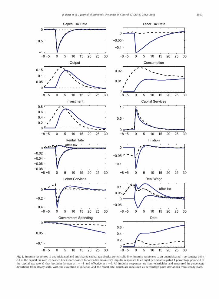
4.1.1. Capital tax rate shocksFig. 2 shows the median impulse responses to an unanticipated (solid line) and an eight period anticipated (dashed line)

one percentage point cut of the capital tax rate.24 The top left panel shows the impulse response for the capital tax rate thatis shocked. In order to deal with the correlation of the tax shocks, we use a Cholesky ordering with capital taxes ordered

21 Compare the working paper version Born et al. (2011), which featured no endogenous feedback, but a considerable estimated output response ofmonetary policy.

22 The high persistence of the labor tax rate has, for example, been documented in Cardia et al. (2003).23 Due to space constraints, the discussion of the government spending shock is relegated to the Online Appendix. In general, the responses to the

surprise government shock are similar to the responses to a spending “news”-shock in Ramey (2011). Although Ramey (2011)-shocks are expected changesin defense spending, spending actually starts rising one quarter after the announcement. Thus, the spending “news”-variable more closely corresponds to asurprise shock in our framework. As in her study, spending, output, hours and labor income taxes rise, while consumption and investment fall. Moreover,the implied peak multiplier in her study is between 1.1 and 1.2, while it is about 0.9 in our baseline model.

24 For both shocks, this roughly corresponds to a one standard deviation shock as s0τk ¼ 0:929% and s8τk ¼ 1:078%.

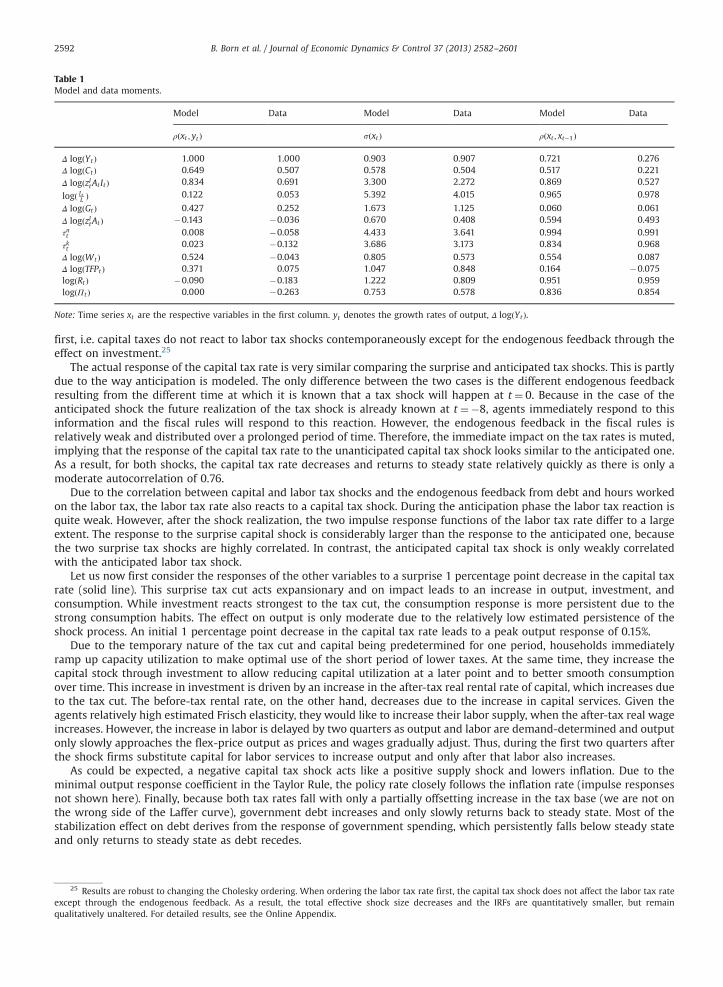
Table 1Model and data moments.

Model Data Model Data Model Data

ρðxt ; yt Þ sðxt Þ ρðxt ; xt�1Þ

Δ logðYt Þ 1.000 1.000 0.903 0.907 0.721 0.276Δ logðCt Þ 0.649 0.507 0.578 0.504 0.517 0.221Δ logðzItAt It Þ 0.834 0.691 3.300 2.272 0.869 0.527

logð LtL Þ 0.122 0.053 5.392 4.015 0.965 0.978

Δ logðGt Þ 0.427 0.252 1.673 1.125 0.060 0.061Δ logðzItAt Þ �0.143 �0.036 0.670 0.408 0.594 0.493τnt 0.008 �0.058 4.433 3.641 0.994 0.991

τkt 0.023 �0.132 3.686 3.173 0.834 0.968

Δ logðWt Þ 0.524 �0.043 0.805 0.573 0.554 0.087Δ logðTFPt Þ 0.371 0.075 1.047 0.848 0.164 �0.075logðRt Þ �0.090 �0.183 1.222 0.809 0.951 0.959logðΠt Þ 0.000 �0.263 0.753 0.578 0.836 0.854

Note: Time series xt are the respective variables in the first column. yt denotes the growth rates of output, Δ logðYt Þ.

B. Born et al. / Journal of Economic Dynamics & Control 37 (2013) 2582–26012592

first, i.e. capital taxes do not react to labor tax shocks contemporaneously except for the endogenous feedback through theeffect on investment.25

The actual response of the capital tax rate is very similar comparing the surprise and anticipated tax shocks. This is partlydue to the way anticipation is modeled. The only difference between the two cases is the different endogenous feedbackresulting from the different time at which it is known that a tax shock will happen at t ¼ 0. Because in the case of theanticipated shock the future realization of the tax shock is already known at t ¼�8, agents immediately respond to thisinformation and the fiscal rules will respond to this reaction. However, the endogenous feedback in the fiscal rules isrelatively weak and distributed over a prolonged period of time. Therefore, the immediate impact on the tax rates is muted,implying that the response of the capital tax rate to the unanticipated capital tax shock looks similar to the anticipated one.As a result, for both shocks, the capital tax rate decreases and returns to steady state relatively quickly as there is only amoderate autocorrelation of 0.76.

Due to the correlation between capital and labor tax shocks and the endogenous feedback from debt and hours workedon the labor tax, the labor tax rate also reacts to a capital tax shock. During the anticipation phase the labor tax reaction isquite weak. However, after the shock realization, the two impulse response functions of the labor tax rate differ to a largeextent. The response to the surprise capital shock is considerably larger than the response to the anticipated one, becausethe two surprise tax shocks are highly correlated. In contrast, the anticipated capital tax shock is only weakly correlatedwith the anticipated labor tax shock.

Let us now first consider the responses of the other variables to a surprise 1 percentage point decrease in the capital taxrate (solid line). This surprise tax cut acts expansionary and on impact leads to an increase in output, investment, andconsumption. While investment reacts strongest to the tax cut, the consumption response is more persistent due to thestrong consumption habits. The effect on output is only moderate due to the relatively low estimated persistence of theshock process. An initial 1 percentage point decrease in the capital tax rate leads to a peak output response of 0.15%.

Due to the temporary nature of the tax cut and capital being predetermined for one period, households immediatelyramp up capacity utilization to make optimal use of the short period of lower taxes. At the same time, they increase thecapital stock through investment to allow reducing capital utilization at a later point and to better smooth consumptionover time. This increase in investment is driven by an increase in the after-tax real rental rate of capital, which increases dueto the tax cut. The before-tax rental rate, on the other hand, decreases due to the increase in capital services. Given theagents relatively high estimated Frisch elasticity, they would like to increase their labor supply, when the after-tax real wageincreases. However, the increase in labor is delayed by two quarters as output and labor are demand-determined and outputonly slowly approaches the flex-price output as prices and wages gradually adjust. Thus, during the first two quarters afterthe shock firms substitute capital for labor services to increase output and only after that labor also increases.

As could be expected, a negative capital tax shock acts like a positive supply shock and lowers inflation. Due to theminimal output response coefficient in the Taylor Rule, the policy rate closely follows the inflation rate (impulse responsesnot shown here). Finally, because both tax rates fall with only a partially offsetting increase in the tax base (we are not onthe wrong side of the Laffer curve), government debt increases and only slowly returns back to steady state. Most of thestabilization effect on debt derives from the response of government spending, which persistently falls below steady stateand only returns to steady state as debt recedes.

25 Results are robust to changing the Cholesky ordering. When ordering the labor tax rate first, the capital tax shock does not affect the labor tax rateexcept through the endogenous feedback. As a result, the total effective shock size decreases and the IRFs are quantitatively smaller, but remainqualitatively unaltered. For detailed results, see the Online Appendix.

−8 −5 0 5 10 15 20 25 30−1

−0.5

0

Capital Tax Rate

−8 −5 0 5 10 15 20 25 30

−0.1

−0.05

0

Labor Tax Rate

−8 −5 0 5 10 15 20 25 30

0

0.05

0.1

0.15

Output

−8 −5 0 5 10 15 20 25 300

0.01

0.02

Consumption

−8 −5 0 5 10 15 20 25 300

0.20.40.60.8

Investment

−8 −5 0 5 10 15 20 25 300

0.5

1

Capital Services

−8 −5 0 5 10 15 20 25 30−0.08−0.06−0.04−0.02

0

Rental Rate

−8 −5 0 5 10 15 20 25 30

−0.1

−0.05

0

−8 −5 0 5 10 15 20 25 30−0.4

−0.2

0

Labor Services

−8 −5 0 5 10 15 20 25 30

−0.05

0

0.05

0.1

Real Wage

−8 −5 0 5 10 15 20 25 30

−0.1

−0.05

0Government Spending

−8 −5 0 5 10 15 20 25 300

0.2

0.4

0.6

Debt

after tax

after tax

Fig. 2. Impulse responses to unanticipated and anticipated capital tax shocks. Notes: solid line: impulse responses to an unanticipated 1 percentage pointcut of the capital tax rate τkt ; dashed line (short-dashed for after-tax measures): impulse responses to an eight period anticipated 1 percentage point cut ofthe capital tax rate τkt that becomes known at t ¼�8 and effective at t ¼ 0. All impulse responses are semi-elasticities and measured in percentagedeviations from steady state, with the exception of inflation and the rental rate, which are measured as percentage point deviations from steady state.

B. Born et al. / Journal of Economic Dynamics & Control 37 (2013) 2582–2601 2593

B. Born et al. / Journal of Economic Dynamics & Control 37 (2013) 2582–26012594

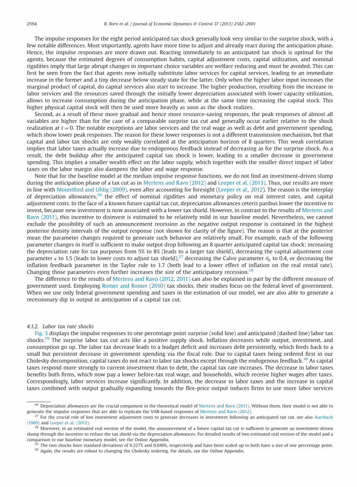
The impulse responses for the eight period anticipated tax shock generally look very similar to the surprise shock, with afew notable differences. Most importantly, agents have more time to adjust and already react during the anticipation phase.Hence, the impulse responses are more drawn out. Reacting immediately to an anticipated tax shock is optimal for theagents, because the estimated degrees of consumption habits, capital adjustment costs, capital utilization, and nominalrigidities imply that large abrupt changes in important choice variables are welfare reducing and must be avoided. This canfirst be seen from the fact that agents now initially substitute labor services for capital services, leading to an immediateincrease in the former and a tiny decrease below steady state for the latter. Only when the higher labor input increases themarginal product of capital, do capital services also start to increase. The higher production, resulting from the increase inlabor services and the resources saved through the initially lower depreciation associated with lower capacity utilization,allows to increase consumption during the anticipation phase, while at the same time increasing the capital stock. Thishigher physical capital stock will then be used more heavily as soon as the shock realizes.

Second, as a result of these more gradual and hence more resource-saving responses, the peak responses of almost allvariables are higher than for the case of a comparable surprise tax cut and generally occur earlier relative to the shockrealization at t ¼ 0. The notable exceptions are labor services and the real wage as well as debt and government spending,which show lower peak responses. The reason for these lower responses is not a different transmission mechanism, but thatcapital and labor tax shocks are only weakly correlated at the anticipation horizon of 8 quarters. This weak correlationimplies that labor taxes actually increase due to endogenous feedback instead of decreasing as for the surprise shock. As aresult, the debt buildup after the anticipated capital tax shock is lower, leading to a smaller decrease in governmentspending. This implies a smaller wealth effect on the labor supply, which together with the smaller direct impact of labortaxes on the labor margin also dampens the labor and wage response.

Note that for the baseline model at the median impulse response functions, we do not find an investment-driven slumpduring the anticipation phase of a tax cut as in Mertens and Ravn (2012) and Leeper et al. (2013). Thus, our results are morein line with Mountford and Uhlig (2009), even after accounting for foresight (Leeper et al., 2012). The reason is the interplayof depreciation allowances,26 the effect of nominal rigidities and monetary policy on real interest rates, and capitaladjustment costs. In the face of a known future capital tax cut, depreciation allowances ceteris paribus lower the incentive toinvest, because new investment is now associated with a lower tax shield. However, in contrast to the results of Mertens andRavn (2011), this incentive to disinvest is estimated to be relatively mild in our baseline model. Nevertheless, we cannotexclude the possibility of such an announcement recession as the negative output response is contained in the highestposterior density intervals of the output response (not shown for clarity of the figure). The reason is that at the posteriormean the parameter changes required to generate such behavior are relatively small. For example, each of the followingparameter changes in itself is sufficient to make output drop following an 8 quarter anticipated capital tax shock: increasingthe depreciation rate for tax purposes from 5% to 8% (leads to a larger tax shield), decreasing the capital adjustment costparameter κ to 1.5 (leads to lower costs to adjust tax shield),27 decreasing the Calvo parameter θp to 0.4, or decreasing theinflation feedback parameter in the Taylor rule to 1.7 (both lead to a lower effect of inflation on the real rental rate).Changing those parameters even further increases the size of the anticipatory recession.28

The difference to the results of Mertens and Ravn (2012, 2011) can also be explained in part by the different measure ofgovernment used. Employing Romer and Romer (2010) tax shocks, their studies focus on the federal level of government.When we use only federal government spending and taxes in the estimation of our model, we are also able to generate arecessionary dip in output in anticipation of a capital tax cut.

4.1.2. Labor tax rate shocksFig. 3 displays the impulse responses to one percentage point surprise (solid line) and anticipated (dashed line) labor tax

shocks.29 The surprise labor tax cut acts like a positive supply shock. Inflation decreases while output, investment, andconsumption go up. The labor tax decrease leads to a budget deficit and increases debt persistently, which feeds back to asmall but persistent decrease in government spending via the fiscal rule. Due to capital taxes being ordered first in ourCholesky decomposition, capital taxes do not react to labor tax shocks except through the endogenous feedback.30 As capitaltaxes respond more strongly to current investment than to debt, the capital tax rate increases. The decrease in labor taxesbenefits both firms, which now pay a lower before-tax real wage, and households, which receive higher wages after taxes.Correspondingly, labor services increase significantly. In addition, the decrease in labor taxes and the increase in capitaltaxes combined with output gradually expanding towards the flex-price output induces firms to use more labor services

26 Depreciation allowances are the crucial component in the theoretical model of Mertens and Ravn (2011). Without them, their model is not able togenerate the impulse responses that are able to replicate the VAR-based responses of Mertens and Ravn (2012).

27 For the crucial role of low investment adjustment costs to generate decreases in investment following an anticipated tax cut, see also Auerbach(1989) and Leeper et al. (2012).

28 Moreover, in an estimated real version of the model, the announcement of a future capital tax cut is sufficient to generate an investment-drivenslump through the incentive to reduce the tax shield via the depreciation allowances. For detailed results of two estimated real version of the model and acomparison to our baseline monetary model, see the Online Appendix.

29 The two shocks have standard deviations of 0.227% and 0.049%, respectively and have been scaled up to both have a size of one percentage point.30 Again, the results are robust to changing the Cholesky ordering. For details, see the Online Appendix.

−8 −5 0 5 10 15 20 25 30

−0.05

0

0.05

0.1

Capital Tax Rate

−8 −5 0 5 10 15 20 25 30−1

−0.5

0

Labor Tax Rate

−8 −5 0 5 10 15 20 25 30

0

0.2

0.4

Output

−8 −5 0 5 10 15 20 25 300

0.05

0.1

0.15

Consumption

−8 −5 0 5 10 15 20 25 30−0.5

00.5

11.5

Investment

−8 −5 0 5 10 15 20 25 30

−0.10

0.10.2

Capital Services

−8 −5 0 5 10 15 20 25 30−0.01

0

0.01

Rental Rate

−8 −5 0 5 10 15 20 25 30

−0.06−0.04−0.02

00.02

−8 −5 0 5 10 15 20 25 30−0.2

0

0.2

0.4

Labor Services

−8 −5 0 5 10 15 20 25 30

0

0.5

1

Real Wage

−8 −5 0 5 10 15 20 25 30

−0.4

−0.2

0Government Spending

−8 −5 0 5 10 15 20 25 300

1

2

3

Debt

after tax

after tax

Fig. 3. Impulse responses to unanticipated and anticipated labor tax shocks. Notes: See Fig. 2.

B. Born et al. / Journal of Economic Dynamics & Control 37 (2013) 2582–2601 2595

instead of capital services. The decrease in capital services stems from a drop in capacity utilization, which overcompensatesthe increase in the capital stock driven by consumption smoothing. Only when the initial burst of deflation starts subsidingdo markups return to their steady state value and do capital services catch up and finally rise above steady state.

B. Born et al. / Journal of Economic Dynamics & Control 37 (2013) 2582–26012596

The anticipated labor tax shock also acts expansionary, but already upon announcement. As explained above, agents havemore time to adjust and save resource and utility costs associated with abruptly changing their behavior. Therefore, theimpulse responses are more drawn out and have a higher peak than for the surprise shock. Due to the smaller relativechange in labor and capital taxation, both labor and capital services increase during the anticipation phase without muchsubstitution taking place. This changes upon realization of the labor tax cut, when firms switch from capital to labor, withboth inputs still being well above steady state.

Initially, due to agents wanting to expand the future capital stock and to consume more immediately due to consumptionsmoothing, inflation slightly increases and then slowly subsides when the production factors capital and labor expand.Inflation only picks up when the labor tax shock realizes, before subsiding again.

4.2. Variance decomposition

We use our DSGE-based estimation approach to analyze the quantitative importance of the different anticipated andsurprise shocks for explaining business cycles. To this end, we compute conditional and unconditional forecast errorvariance decompositions for the growth rates of output, consumption, investment, hours, wages, the federal funds rate,inflation, labor and capital tax rates, and government spending (see Table A3).31 We find that fiscal foresight plays amoderate role in explaining business cycle fluctuations. Specifically, using full information Bayesian estimation andaccounting for different kinds of shocks, we find that anticipated government spending is the fiscal variable with the largesteffect on output variance. It is responsible for 13% of output variance, which is close to the 16% found by Forni and Gambetti(2010), who use a factor VAR to deal with fiscal foresight and also consider total government data. However, this value issomewhat larger than the 6% found by Schmitt-Grohé and Uribe (2012) in their RBC-DSGE model without endogenous fiscalfeedback.32

We find that capital tax shocks and, in particular, news about capital taxes explain less than 2% of output growthfluctuations in our baseline model, while news about labor tax shocks do not matter at all. This compares to an outputvariance contribution of tax shocks of about 20% to 27% in the VAR study of Mertens and Ravn (2012). However, their studyuses Romer and Romer (2010) tax shocks and is thus focused on the federal level. Whenwe estimated our baseline model onfederal fiscal data only, tax shocks account for 24% of output fluctuations (see the results and discussion in Section 4.3).

Regarding the evidence on the effects of news shocks on the business cycles, our finding that about 50% of the variance ofoutput growth can be attributed to anticipated shocks is on the upper end of estimates found in Forni et al. (2011), Barskyand Sims (2011), and Kurmann and Otrok (forthcoming). The news shocks that matter most are news about non-stationarytechnology, which account for 13% to 22% of the variance of output and consumption. With a variance share of 19% to 22%,news about stationary TFP is especially important in explaining the variability of investment growth. But it also contributessignificantly to the variance of output (12% to 15%). Using a factor model, Forni et al. (2011) find that around 20% of outputvolatility is explained by technology and 10% by news about technology, while Barsky and Sims (2011), in a VAR, attribute10% to 40% to news shocks. Kurmann and Otrok (forthcoming) study the term-structure of interest rates in a VAR and findthat non-stationary TFP news, the only news shocks they consider, account for about 50% of output volatility.

Fujiwara et al. (2011) and Khan and Tsoukalas (2012), using an estimated DSGE model with nominal rigidities, find atechnology news contribution to output variance of 8.5% and 1.6%, respectively, while Schmitt-Grohé and Uribe (2012) in thecontext of a real model find that news about technology account for about 10% of output variance. Our own estimate of atechnology news contribution of 33% is closer to the monetary DGSE model of Davis (2007) with 20% to 50% of outputvariance attributed to technology news and the 50% in the VAR of Kurmann and Otrok (forthcoming).

Allowing anticipation not only for TFP but also for other shocks leads to a higher relative contribution of news shocks.Whereas the contribution of anticipated shocks in the study by Fujiwara et al. (2011) ranges from 4% (to the variance ofinvestment) to 15% (to inflation volatility), we find contributions of anticipated shocks (combining all shocks) between 29%(consumption volatility) and 60% (variance of the nominal interest rate). This difference to Fujiwara et al. (2011) is mostlydue to the fact that Fujiwara et al. (2011) assume the presence of a deterministic linear trend and thus do not allow forchanges in trend growth. In contrast, most of the importance of TFP news shocks in our model is driven by the non-stationary, i.e. trend, shock. The difference to the results in Khan and Tsoukalas (2012) seems to be due to our differentspecification of the investment specific technology shocks (see below), as in their study the contemporaneous investmentspecific technology shock accounts for 68% and 87% of output and investment variability, thus hardly leaving room for othershocks at all.33

31 For ease of exposition we have combined the two anticipated shock components into one and left out the anticipated stationary investment-specificshocks that contribute less than 0.1% to the variance of the variables. Full tables can be found in the Online Appendix.

32 Estimating a version of the Schmitt-Grohé and Uribe (2012) model with fiscal feedback and including an anticipated preference shock as in theirmodel, we find that only surprise spending shocks matter with a contribution to output variance of about 12%. When adding a nominal block, the modelmoments of the fiscal and technological variables move closer to the empirical data, while at the same time the importance of the anticipated governmentspending shock increases at the cost of the surprise one. This better model fit suggests the importance of nominal rigidities and the interaction of fiscalpolicy with monetary policy to account for the empirically observed data. For more details, see the Online Appendix.

33 A further confounding factor is that Khan and Tsoukalas (2012) do not use TFP as an observable, while we do.

B. Born et al. / Journal of Economic Dynamics & Control 37 (2013) 2582–2601 2597

Turning to the role of unanticipated shocks, we see that while the investment-specific technology shock has beenidentified as an important driver of business cycles by previous studies (Fisher, 2006; Davis, 2007; Justiniano et al., 2010a), itis of lesser importance in our case and contributes a smaller fraction to fluctuations than TFP shocks. The contributions ofnon-stationary investment-specific productivity vary between 2.3% (e.g. output) and 6% (inflation), whereas stationaryinvestment-specific technology explains less than 1%. The difference to the previous studies' finding of a high contribution ofinvestment-specific technology stems from our decision to include the relative price of investment as an observable. Recentstudies, which include the relative price of investment as an observable, find similarly small contributions of investment-specific technology (Justiniano et al., 2011; Schmitt-Grohé and Uribe, 2012).34 However, we have to stress that both thestationary as well as the non-stationary investment-specific productivity shock pertain to the relative price of investmentand are, accordingly, mapped to this observable. Thus, our stationary investment-specific technology shock is not directlycomparable to the stationary investment-specific technology shock in Schmitt-Grohé and Uribe (2012), which is rather amarginal efficiency of investment (MEI) shock as in Justiniano et al. (2011). This could explain the differing results regardingthe effects of this particular shock for output with 20% in their case vs. less than 1% in our model. Following the criticism ofChari et al. (2009), we abstain from including this additional type of disturbance, as it has no clear structural interpretation(apart from maybe being related to financial disturbances) in our one-sector model and its inclusion would not bedisciplined by observable data.35

4.3. Fiscal policy at the federal level

One could argue that nationwide shocks have different implications than state level shocks. To better judge the effect offiscal policy measures at the federal level, like e.g. stimulus packages, holding the revenues and expenditures at thesubnational level constant (something that might theoretically be done by giving appropriate transfers to the states), wehave re-estimated our model with fiscal data from the federal level only.

The importance of fiscal foresight increases considerably as can be seen from the lower panel of Table A3. Fiscal foresightnow explains 37% of the unconditional variance of output. Particularly important is foresight about government spending(22% of output variance), followed by anticipated labor tax rates (11%), and capital taxes (4%). While in our baseline modelsurprise and anticipated labor tax shocks did not play a big role in explaining the variance of the variables considered, theyare now an important driver of variability. This is mostly due to three changes in the estimated parameter values (see thelast column of Tables A2 and A3). First, labor tax shocks are estimated to be a lot more persistent at 0.998 compared to 0.94.This together with the second element, the lower Frisch elasticity of labor supply (sl ¼ 2:598 compared to 0.786 in thebaseline model), implies more persistent responses of the labor supply. Third, the feedback of capital taxes to investment isestimated to be negative (ϕkI ¼�0:009). Due to those three parameter changes, an investment increase after a decrease inlabor taxes leads to a rise in labor and thereby the marginal product of capital. A decrease in capital taxation further propelsthis boom. This generates a very strong amplification mechanism as shown in the impulse responses discussed below.

If we consider the model estimated on federal fiscal data instead of total government data, the impulse responses to bothsurprise and anticipated government spending shocks hardly change neither quantitatively nor qualitatively.36 For the labortax shock, the impulse responses change quantitatively for both surprise and anticipated shocks, but are very similarqualitatively. The main difference relates to capital taxes and explains the quantitative differences: because capital taxes areestimated to decrease when investment increases, the boom in investment, consumption, and output generated by the labortax cut is further propelled as capital taxes decrease. In contrast, for the model with total government, an endogenouscapital tax increase dampened the output effect. Moreover, due to the stronger boom, the effect on government debt islower and even turns negative after 12 quarters for the surprise shock and 4 quarters after announcement for theanticipated shock. Via feedback, this lower debt build-up compared to the total government case relatively quickly leads toan additional increase in government spending and thus output. As a result, the labor tax decrease has a very largemultiplier with a peak output response of about 3%.

For the surprise capital tax shock, the impulse responses are both qualitatively and quantitatively similar to the baselineresponses. However, for the anticipated capital tax shock the responses differ strongly from the baseline case. Due to anestimated negative correlation of the anticipated labor and capital tax shocks, the anticipated decrease in capital taxes isassociated with the expectation of an increase in labor taxes. Paired with the lower estimated value of the Frisch elasticitycompared to the general government case, people start decreasing their labor supply immediately, leading to a drop ininvestment and thus generating an investment-driven anticipatory recession. Moreover, due to the persistent increase ingovernment debt and the high persistence of the labor tax rate, the tax burden on labor stays high for a long time, creating ashort-lived boom after the capital tax cut realizes.

34 Models that do not use the relative price of investment as an observable variable usually imply wrong moments for this series (Justiniano et al.,2011). When this problem is eliminated, the variance contribution of investment-specific technology shocks tends to disappear.

35 For details on the importance of measurement error, see the Online Appendix. Measurement error explains about 3% to 10% of the variance of wages,corroborating recent work by Justiniano et al. (2013), who stress the importance of accounting for measurement error in wages. Also not surprisingly, giventhe construction of labor and capital tax rates, measurement error is an important contributor to their variance, explaining 20–30 at short and 1% to 5% atlong horizons.

36 Impulse response plots can be found in the Online Appendix.

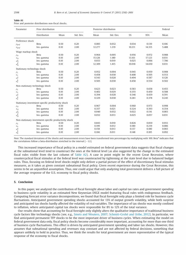
Table A1Prior and posterior distributions non-fiscal shocks.

Parameter Prior distribution Posterior distribution Federal

Distribution Mean Std. Dev. Mean Std. Dev. 5% 95% Mean

Preference shockρpref Beta 0.50 0.20 0.085 0.032 0.034 0.139 0.106spref Inv.-gamma 0.10 2.00 12.277 1.219 10.211 14.315 5.488

Wage markup shockρw Beta 0.50 0.20 0.964 0.005 0.956 0.972 0.988sw Inv.-gamma 0.10 2.00 15.128 1.180 13.161 17.123 0.031s4w Inv.-gamma 0.10 2.00 0.033 0.019 0.025 0.066 7.786

s8w Inv.-gamma 0.10 2.00 12.309 1.415 10.018 14.650 0.031

Stationary technology shockρz Beta 0.50 0.20 0.952 0.004 0.945 0.959 0.908sz Inv.-gamma 0.10 2.00 0.458 0.030 0.408 0.505 0.553s4z Inv.-gamma 0.10 2.00 0.543 0.028 0.494 0.587 0.128

s8z Inv.-gamma 0.10 2.00 0.505 0.030 0.458 0.554 0.502

Non-stationary technology shockρx Beta 0.50 0.20 0.623 0.023 0.583 0.658 0.455sx Inv.-gamma 0.10 2.00 0.402 0.029 0.355 0.450 0.588s4x Inv.-gamma 0.10 2.00 0.394 0.028 0.346 0.439 0.591

s8x Inv.-gamma 0.10 2.00 0.329 0.030 0.281 0.378 0.245

Stationary investment-specific productivity shockρzI Beta 0.50 0.20 0.967 0.004 0.960 0.973 0.998szI Inv.-gamma 0.10 2.00 0.357 0.021 0.324 0.393 0.354s4zI Inv.-gamma 0.10 2.00 0.040 0.032 0.022 0.116 0.083

s8zI Inv.-gamma 0.10 2.00 0.032 0.013 0.025 0.057 0.031

Non-stationary investment-specific productivity shockρa Beta 0.50 0.20 0.843 0.010 0.826 0.859 0.955sa Inv.-gamma 0.10 2.00 0.199 0.012 0.180 0.219 0.086s4a Inv.-gamma 0.10 2.00 0.158 0.013 0.137 0.180 0.065

s8a Inv.-gamma 0.10 2.00 0.166 0.011 0.148 0.185 0.092

Note: The standard deviations of the shocks and measurement errors have been transformed into percentages by multiplying with 100. Betan indicates thatthe correlations follow a beta-distribution stretched to the interval [�1,1].

B. Born et al. / Journal of Economic Dynamics & Control 37 (2013) 2582–26012598

This increased importance of fiscal policy in a model estimated on federal government data suggests that fiscal changesat the subnational level tend to counteract the ones at the federal level (as also suggested by the change in the estimatedfiscal rules visible from the last column of Table A2). A case in point might be the recent Great Recession, wherecountercyclical fiscal stimulus at the federal level was counteracted by tightening at the state level due to balanced budgetrules. Thus, focusing on federal level shocks might only deliver a partial picture of the effect of discretionary fiscal stimulusmeasures, as it takes as given constant subnational fiscal policy. Given recent experience during the Great Recession, thisseems to be an unjustified assumption. Thus, one could argue that only analyzing total government delivers a full picture ofthe average response of the U.S. economy to fiscal policy shocks.

5. Conclusion

In this paper, we analyzed the contribution of fiscal foresight about labor and capital tax rates and government spendingto business cycle volatility in an estimated New Keynesian DSGE model featuring fiscal rules with endogenous feedback.Computing forecast error variance decompositions, we found that fiscal foresight only plays a limited role for business cyclefluctuations. Anticipated government spending shocks accounted for 13% of output growth volatility, while both surpriseand anticipated tax shocks hardly affected the volatility of real variables. The importance of tax shocks was mostly confinedto inflation, where anticipated capital tax shocks were responsible for 8% to 12% of the total variance.

Our results show that accounting for fiscal foresight only slightly alters the qualitative importance of traditional businesscycle factors like technology shocks (see, e.g., Smets and Wouters, 2007; Schmitt-Grohé and Uribe, 2012). In particular, wefind anticipated permanent TFP shocks to be the most important driver of business cycles. When estimating the model onfederal government data only, fiscal policy shocks become considerably more important, accounting for more than one thirdof business cycle fluctuations. This effect is driven by anticipated government spending and labor tax shocks. However, thisassumes that subnational spending and revenues stay constant and are not affected by federal decisions, something thatappears unlikely to hold in practice. Thus, we think the results for total government are more representative of the typicalresponse of the economy to fiscal shocks.

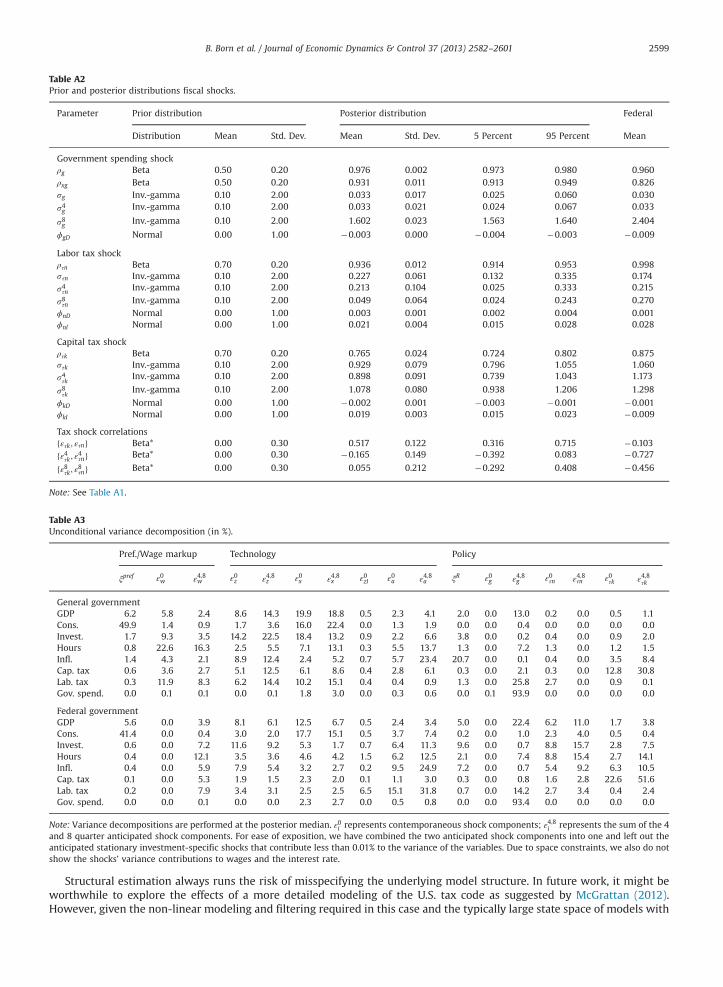
Table A2Prior and posterior distributions fiscal shocks.

Parameter Prior distribution Posterior distribution Federal

Distribution Mean Std. Dev. Mean Std. Dev. 5 Percent 95 Percent Mean

Government spending shockρg Beta 0.50 0.20 0.976 0.002 0.973 0.980 0.960ρxg Beta 0.50 0.20 0.931 0.011 0.913 0.949 0.826sg Inv.-gamma 0.10 2.00 0.033 0.017 0.025 0.060 0.030s4g Inv.-gamma 0.10 2.00 0.033 0.021 0.024 0.067 0.033

s8g Inv.-gamma 0.10 2.00 1.602 0.023 1.563 1.640 2.404

ϕgD Normal 0.00 1.00 �0.003 0.000 �0.004 �0.003 �0.009

Labor tax shockρτn Beta 0.70 0.20 0.936 0.012 0.914 0.953 0.998sτn Inv.-gamma 0.10 2.00 0.227 0.061 0.132 0.335 0.174s4τn Inv.-gamma 0.10 2.00 0.213 0.104 0.025 0.333 0.215

s8τn Inv.-gamma 0.10 2.00 0.049 0.064 0.024 0.243 0.270ϕnD Normal 0.00 1.00 0.003 0.001 0.002 0.004 0.001ϕnl Normal 0.00 1.00 0.021 0.004 0.015 0.028 0.028

Capital tax shockρτk Beta 0.70 0.20 0.765 0.024 0.724 0.802 0.875sτk Inv.-gamma 0.10 2.00 0.929 0.079 0.796 1.055 1.060s4τk Inv.-gamma 0.10 2.00 0.898 0.091 0.739 1.043 1.173

s8τk Inv.-gamma 0.10 2.00 1.078 0.080 0.938 1.206 1.298

ϕkD Normal 0.00 1.00 �0.002 0.001 �0.003 �0.001 �0.001ϕkI Normal 0.00 1.00 0.019 0.003 0.015 0.023 �0.009

Tax shock correlationsfετk ; ετng Beta* 0.00 0.30 0.517 0.122 0.316 0.715 �0.103fε4τk ; ε4τng Beta* 0.00 0.30 �0.165 0.149 �0.392 0.083 �0.727

fε8τk ; ε8τng Beta* 0.00 0.30 0.055 0.212 �0.292 0.408 �0.456

Note: See Table A1.

Table A3Unconditional variance decomposition (in %).

Pref./Wage markup Technology Policy

ξpref ε0w ε4;8w ε0z ε4;8z ε0x ε4;8x ε0zI ε0a ε4;8a ξR ε0g ε4;8g ε0τn ε4;8τn ε0τk ε4;8τk

General governmentGDP 6.2 5.8 2.4 8.6 14.3 19.9 18.8 0.5 2.3 4.1 2.0 0.0 13.0 0.2 0.0 0.5 1.1Cons. 49.9 1.4 0.9 1.7 3.6 16.0 22.4 0.0 1.3 1.9 0.0 0.0 0.4 0.0 0.0 0.0 0.0Invest. 1.7 9.3 3.5 14.2 22.5 18.4 13.2 0.9 2.2 6.6 3.8 0.0 0.2 0.4 0.0 0.9 2.0Hours 0.8 22.6 16.3 2.5 5.5 7.1 13.1 0.3 5.5 13.7 1.3 0.0 7.2 1.3 0.0 1.2 1.5Infl. 1.4 4.3 2.1 8.9 12.4 2.4 5.2 0.7 5.7 23.4 20.7 0.0 0.1 0.4 0.0 3.5 8.4Cap. tax 0.6 3.6 2.7 5.1 12.5 6.1 8.6 0.4 2.8 6.1 0.3 0.0 2.1 0.3 0.0 12.8 30.8Lab. tax 0.3 11.9 8.3 6.2 14.4 10.2 15.1 0.4 0.4 0.9 1.3 0.0 25.8 2.7 0.0 0.9 0.1Gov. spend. 0.0 0.1 0.1 0.0 0.1 1.8 3.0 0.0 0.3 0.6 0.0 0.1 93.9 0.0 0.0 0.0 0.0

Federal governmentGDP 5.6 0.0 3.9 8.1 6.1 12.5 6.7 0.5 2.4 3.4 5.0 0.0 22.4 6.2 11.0 1.7 3.8Cons. 41.4 0.0 0.4 3.0 2.0 17.7 15.1 0.5 3.7 7.4 0.2 0.0 1.0 2.3 4.0 0.5 0.4Invest. 0.6 0.0 7.2 11.6 9.2 5.3 1.7 0.7 6.4 11.3 9.6 0.0 0.7 8.8 15.7 2.8 7.5Hours 0.4 0.0 12.1 3.5 3.6 4.6 4.2 1.5 6.2 12.5 2.1 0.0 7.4 8.8 15.4 2.7 14.1Infl. 0.4 0.0 5.9 7.9 5.4 3.2 2.7 0.2 9.5 24.9 7.2 0.0 0.7 5.4 9.2 6.3 10.5Cap. tax 0.1 0.0 5.3 1.9 1.5 2.3 2.0 0.1 1.1 3.0 0.3 0.0 0.8 1.6 2.8 22.6 51.6Lab. tax 0.2 0.0 7.9 3.4 3.1 2.5 2.5 6.5 15.1 31.8 0.7 0.0 14.2 2.7 3.4 0.4 2.4Gov. spend. 0.0 0.0 0.1 0.0 0.0 2.3 2.7 0.0 0.5 0.8 0.0 0.0 93.4 0.0 0.0 0.0 0.0

Note: Variance decompositions are performed at the posterior median. ε0i represents contemporaneous shock components; ε4;8i represents the sum of the 4and 8 quarter anticipated shock components. For ease of exposition, we have combined the two anticipated shock components into one and left out theanticipated stationary investment-specific shocks that contribute less than 0.01% to the variance of the variables. Due to space constraints, we also do notshow the shocks’ variance contributions to wages and the interest rate.

B. Born et al. / Journal of Economic Dynamics & Control 37 (2013) 2582–2601 2599

Structural estimation always runs the risk of misspecifying the underlying model structure. In future work, it might beworthwhile to explore the effects of a more detailed modeling of the U.S. tax code as suggested by McGrattan (2012).However, given the non-linear modeling and filtering required in this case and the typically large state space of models with

B. Born et al. / Journal of Economic Dynamics & Control 37 (2013) 2582–26012600

anticipation effects, estimating the effects of fiscal news in such a model will be an extremely challenging computationaltask. Finally, the role of the information structure assumed in the present work should be further scrutinized as theparticular choice of information structures may matter (Leeper and Walker, 2011).

Acknowledgments

We would like to thank Martin Flodén (the editor), two anonymous referees, Zeno Enders, Patrick Hürtgen, GernotMüller, Jörn Tenhofen, Arnoud Stevens, Todd Walker, and seminar audiences in Bonn and Dortmund, as well as participantsat the Doctoral Workshop on Dynamic Macroeconomics 2010, the 2nd Conference on Recent Developments inMacroeconomics, the 2010 Cologne Workshop on Macroeconomics, the 2010 Annual Meeting of the Verein für Socialpolitik,the 2012 SEEK/CEPR Workshop on News, Sentiment, and Confidence in Fluctuations, and the Spring Meeting of YoungEconomists 2012 for helpful comments and discussions. We are grateful to Martín Uribe for providing us with the relativeprice of investment data. All remaining errors are our own. The views of this paper are those of the authors and do notnecessarily represent those of the IMF or IMF policy.

Appendix A. Tables

See Tables A1–A3.

Appendix B. Supplementary data

Supplementary data associated with this article can be found in the online version at http://dx.doi.org.10.1016/j.jedc.2013.06.011.

References

An, S., Schorfheide, F., 2007. Bayesian analysis of DSGE models. Econometric Reviews 26 (2–4), 113–172.Auerbach, A.J., 1989. Tax reform and adjustment costs: the impact on investment and market value. International Economic Review 30 (4), 939–962.Barro, R.J., Redlick, C.J., 2011. Macroeconomic effects from government purchases and taxes. Quarterly Journal of Economics 126 (1), 51–102.Barro, R.J., Sahasakul, C., 1983. Measuring the average marginal tax rate from the individual income tax. Journal of Business 56 (4), 419–452.Barsky, R.B., Sims, E., 2011. News shocks and business cycles. Journal of Monetary Economics 58 (3), 273–289.Baxter, M., King, R.G., 1993. Fiscal policy in general equilibrium. American Economic Review 83 (3), 315–334.Beaudry, P., Portier, F., 2004. An exploration into Pigou's theory of cycles. Journal of Monetary Economics 51 (6), 1183–1216.Beaudry, P., Portier, F., 2006. Stock prices, news, and economic fluctuations. American Economic Review 96 (4), 1293–1307.Blanchard, O.J., Perotti, R., 2002. An empirical characterization of the dynamic effects of changes in government spending and taxes on output. Quarterly

Journal of Economics 117 (4), 1329–1368.Born, B., Peter, A., Pfeifer, J., 2011. Fiscal News and Macroeconomic Volatility. Bonn Econ Discussion Papers 08/2011.Born, B., Pfeifer, J., 2011. Policy Risk and the Business Cycle. Bonn Econ Discussion Papers 06/2011.Calvo, G.A., 1983. Staggered prices in a utility-maximizing framework. Journal of Monetary Economics 12 (3), 383–398.Cardia, E., Kozhaya, N., Ruge-Murcia, F.J., 2003. Distortionary taxation and labor supply. Journal of Money, Credit and Banking 35 (3), 350–373.Chari, V.V., Kehoe, P.J., McGrattan, E.R., 2009. New Keynesian models: not yet useful for policy analysis. American Economic Journal: Macroeconomics 1 (1),

242–266.Chib, S., Ramamurthy, S., 2010. Tailored randomized block MCMC methods with application to DSGE models. Journal of Econometrics 155 (1), 19–38.Christiano, L.J., Eichenbaum, M., Evans, C.L., 2005. Nominal rigidities and the dynamic effects of a shock to monetary policy. Journal of Political Economy

113 (1), 1–45.Christiano, L.J., Ilut, C., Motto, R., Rostagno, M., 2008. Monetary Policy and Stock Market Boom-Bust Cycles. ECB Working Paper Series 955.Christiano, L.J., Trabandt, M., Walentin, K., 2011. Introducing financial frictions and unemployment into a small open economy model. Journal of Economic

Dynamics and Control 35 (12), 1999–2041.Clarida, R., Galí, J., Gertler, M., 2000. Monetary policy rules and macroeconomic stability: evidence and some theory. Quarterly Journal of Economics 115 (1),

147–180.Davis, J.M., 2007. News and the Term Structure in General Equilibrium. Mimeo.Del Negro, M., Schorfheide, F., 2008. Forming priors for DSGE models (and how it affects the assessment of nominal rigidities). Journal of Monetary

Economics 55 (7), 1191–1208.Fernández-Villaverde, J., 2010. The econometrics of DSGE models. SERIEs 1 (1), 3–49.Fernández-Villaverde, J., Guerrón-Quintana, P.A., Kuester, K., Rubio-Ramírez, J., 2011. Fiscal Volatility Shocks and Economic Activity. NBER Working Papers

17317.Fernández-Villaverde, J., Rubio-Ramírez, J.F., Sargent, T.J., Watson, M.W., 2007. ABCs (and Ds) of understanding VARs. American Economic Review 97 (3),

1021–1026.Fisher, J.D., 2006. The dynamic effects of neutral and investment specific technology shocks. Journal of Political Economy 114 (3), 413–451.Forni, L., Monteforte, L., Sessa, L., 2009. The general equilibrium effects of fiscal policy: estimates for the euro area. Journal of Public Economics 93 (3–4),

559–585.Forni, M., Gambetti, L., 2010. Fiscal Foresight and the Effects of Government Spending. CEPR Discussion Papers 7840.Forni, M., Gambetti, L., Sala, L., 2011. No News in Business Cycles. CEPR Discussion Papers 8274.Fujiwara, I., Hirose, Y., Shintani, M., 2011. Can news be a major source of aggregate fluctuations? A Bayesian DSGE approach. Journal of Money, Credit and

Banking 43 (1), 1–29.Galí, J., López-Salido, J.D., Vallés, J., 2007. Understanding the effects of government spending on consumption. Journal of the European Economic

Association 5 (1), 227–270.Galí, J., Smets, F., Wouters, R., 2011. Unemployment in an estimated new Keynesian model. In: NBER Macroeconomics Annual 2011, vol. 26.Gambetti, L., 2012. Government spending news and shocks. Mimeo, Universitat Autonoma de Barcelona.

B. Born et al. / Journal of Economic Dynamics & Control 37 (2013) 2582–2601 2601

Giannone, D., Reichlin, L., 2006. Does information help recovering structural shocks from past observations? Journal of the European Economic Association4 (2–3), 455–465.

Greenwood, J., Hercowitz, Z., Huffman, G.W., 1988. Investment, capacity utilization, and the real business cycle. American Economic Review 78 (3), 402–417.Greenwood, J., Hercowitz, Z., Krusell, P., 1997. Long-run implications of investment-specific technological change. American Economic Review 87 (3),

342–362.Greenwood, J., Hercowitz, Z., Krusell, P., 2000. The role of investment-specific technological change in the business cycle. European Economic Review 44 (1),

91–115.Hansen, L.P., Sargent, T.J., 1991. Two difficulties in interpreting vector autoregressions. In: Lucas, R., Sargent, T. (Eds.), Rational Expectations Econometrics,

pp. 77–119.House, C.L., Shapiro, M.D., 2006. Phased-in tax cuts and economic activity. American Economic Review 96 (5), 1835–1849.Jaimovich, N., Rebelo, S., 2009. Can news about the future drive the business cycle? American Economic Review 99 (4), 1097–1118.Jones, J.B., 2002. Has fiscal policy helped stabilize the postwar U.S. economy? Journal of Monetary Economics 49 (4), 709–746.Justiniano, A., Primiceri, G.E., Tambalotti, A., 2010a. Investment shocks and business cycles. Journal of Monetary Economics 57 (2), 132–145.Justiniano, A., Primiceri, G.E., Tambalotti, A., 2010b. Investment shocks and business cycles, Online Appendix, available at ⟨http://faculty.wcas.northwestern.

edu/�gep575/samm_OnlineAppendix5_gt.pdf⟩ (accessed February 28th, 2010).Justiniano, A., Primiceri, G.E., Tambalotti, A., 2011. Investment shocks and the relative price of investment. Review of Economic Dynamics 14 (1), 102–121.Justiniano, A., Primiceri, G.E., Tambalotti, A., 2013. Is there a trade-off between inflation and output stabilization? American Economic Journal:

Macroeconomics 5 (2), 1–31.Khan, H., Tsoukalas, J., 2012. The quantitative importance of news shocks in estimated DSGE models. Journal of Money, Credit and Banking 44 (8),

1535–1561.King, R.G., Plosser, C.I., Rebelo, S.T., 1988. Production, growth and business cycles: I. The basic neoclassical model. Journal of Monetary Economics 21 (2–3),

195–232.Kliem, M., Kriwoluzky, A., 2012. Toward a Taylor Rule for Fiscal Policy. Mimeo, University of Bonn.Kurmann, A., Otrok, C, forthcoming. News shocks and the slope of the term structure of interest rates. American Economic Review.Leeper, E.M., Plante, M., Traum, N., 2010. Dynamics of fiscal financing in the United States. Journal of Econometrics 156 (2), 304–321.Leeper, E.M., Walker, T.B., 2011. Information flows and news driven business cycles. Review of Economic Dynamics 14 (1), 55–71.Leeper, E.M., Walker, T.B., Yang, S.-C.S., 2012. Fiscal Foresight and Information Flows. Technical appendix.Leeper, E.M., Walker, T.B., Yang, S.-C.S., 2013. Fiscal foresight and information flows. Econometrica 81 (3), 1115–1145.Lubik, T.A., Schorfheide, F., 2007. Do central banks respond to exchange rate movements? A structural investigation. Journal of Monetary Economics 54 (4),

1069–1087.McGrattan, E.R., 1994. The macroeconomic effects of distortionary taxation. Journal of Monetary Economics 33 (3), 573–601.McGrattan, E.R., 2012. Capital taxation during the U.S. great depression. Quarterly Journal of Economics 127 (3), 1515–1550.Mendoza, E.G., Razin, A., Tesar, L.L., 1994. Effective tax rates in macroeconomics: cross-country estimates of tax rates on factor incomes and consumption.

Journal of Monetary Economics 34 (3), 297–323.Mertens, K., Ravn, M.O., 2011. Understanding the aggregate effects of anticipated and unanticipated tax policy shocks. Review of Economic Dynamics 14 (1),

27–54.Mertens, K., Ravn, M.O., 2012. Empirical evidence on the aggregate effects of anticipated and unanticipated U.S. tax policy shocks. American Economic

Journal: Economic Policy 4 (2), 145–181.Monacelli, T., Perotti, R., 2008. Fiscal Policy, Wealth Effects, and Markups. NBER Working Papers 14584.Mountford, A., Uhlig, H., 2009. What are the effects of fiscal policy shocks? Journal of Applied Econometrics 24 (6), 960–992.Nutahara, K., 2010. Internal and external habits and news-driven business cycles. Economics Letters 107, 300–303.Parker, J.A., 1999. The reaction of household consumption to predictable changes in social security taxes. American Economic Review 89 (4), 959–973.Poterba, J.M., 1988. Are consumers forward looking? Evidence from fiscal experiments. American Economic Review 78 (2), 413–418.Ramey, V.A., 2011. Identifying government spending shocks: it's all in the timing. Quarterly Journal of Economics 126 (1), 1–50.Romer, C.D., Romer, D.H., 2010. The macroeconomic effects of tax changes: estimates based on a new measure of fiscal shocks. American Economic Review

100 (3), 763–801.Schmitt-Grohé, S., Uribe, M., 2006. Optimal fiscal and monetary policy in a medium-scale macroeconomic model. In: NBER Macroeconomics Annual 2005,

vol. 20, pp. 383–462.Schmitt-Grohé, S., Uribe, M., 2012. What's news in business cycles. Econometrica 80 (6), 2733–2764.Sims, E., 2012. Non-invertibilities and structural VARs. Advances in Econometrics 28, 81–135.Smets, F., Wouters, R., 2003. An estimated dynamic stochastic general equilibrium model of the euro area. Journal of the European Economic Association 1

(5), 1123–1175.Smets, F., Wouters, R., 2007. Shocks and frictions in US business cycles: a Bayesian DSGE approach. American Economic Review 97 (3), 586–606.Yang, S.-C.S., 2005. Quantifying tax effects under policy foresight. Journal of Monetary Economics 52 (8), 1557–1568.Yun, T., 1996. Nominal price rigidity, money supply endogeneity, and business cycles. Journal of Monetary Economics 37 (2), 345–370.