first-principles electronic-state calculation code by
TRANSCRIPT

First-Principles Electronic-State
Calculation Code
by Pseudopotential Method
Osaka2002 nano
VOL. I
– Basic Usage –
First Edition
Koun SHIRAI
ISIR, Osakak University
2 November 2004

1
History
Rev. 0.7 04 March 2003Rev. 0.9 18 December 2003Rev. 1.0 04 February 2004 Rev. 1.1 02 November 2004
Contents
Introduction 5
1 THEORY 81.1 Density functional method . . . . . . . . . . . . . . . . . . . . 81.2 Local Density Approximation . . . . . . . . . . . . . . . . . . 111.3 Pseudopotential Approximation [8] . . . . . . . . . . . . . . . 111.4 Plane-wave expansion . . . . . . . . . . . . . . . . . . . . . . 141.5 Plane-wave cutoff . . . . . . . . . . . . . . . . . . . . . . . . . 161.6 k-space summation . . . . . . . . . . . . . . . . . . . . . . . . 171.7 Conjugate gradient method in Kohn-Sham functional . . . . . 191.8 Fast Fourier transform . . . . . . . . . . . . . . . . . . . . . . 241.9 Hellmann-Faynman forces and stresses . . . . . . . . . . . . . 25
2 Load Map 272.1 Overview . . . . . . . . . . . . . . . . . . . . . . . . . . . . . 272.2 Preparation . . . . . . . . . . . . . . . . . . . . . . . . . . . . 27
2.2.1 machine dependence . . . . . . . . . . . . . . . . . . . 302.3 Input parameters . . . . . . . . . . . . . . . . . . . . . . . . . 31
2.3.1 Input options . . . . . . . . . . . . . . . . . . . . . . . 31
3 Atomic pseudopotentials 333.1 input file . . . . . . . . . . . . . . . . . . . . . . . . . . . . . . 333.2 execution . . . . . . . . . . . . . . . . . . . . . . . . . . . . . 36
4 Construction of crystals 404.1 Input of crystal data . . . . . . . . . . . . . . . . . . . . . . . 404.2 Execution of cryst . . . . . . . . . . . . . . . . . . . . . . . . 444.3 Control parameters . . . . . . . . . . . . . . . . . . . . . . . . 464.4 Graphics display of crystal structure . . . . . . . . . . . . . . 47
2
CONTENTS 3
5 Ground states of electronic structures (I) 495.1 inip . . . . . . . . . . . . . . . . . . . . . . . . . . . . . . . . 49
5.1.1 specail k-point sampling . . . . . . . . . . . . . . . . . 515.1.2 Cutoff radius of planewaves . . . . . . . . . . . . . . . 54
5.2 pwm . . . . . . . . . . . . . . . . . . . . . . . . . . . . . . . . 565.2.1 SCF calculation . . . . . . . . . . . . . . . . . . . . . . 565.2.2 Interpretation . . . . . . . . . . . . . . . . . . . . . . . 585.2.3 Recalculation . . . . . . . . . . . . . . . . . . . . . . . 645.2.4 Display of charge density . . . . . . . . . . . . . . . . 655.2.5 Cases of wrong convergence . . . . . . . . . . . . . . . 685.2.6 Related options . . . . . . . . . . . . . . . . . . . . . . 69
6 Ground-States of Solids (II) 726.1 Atom Optimization . . . . . . . . . . . . . . . . . . . . . . . . 72
6.1.1 Preparation of calculation . . . . . . . . . . . . . . . . 736.1.2 Interpretation . . . . . . . . . . . . . . . . . . . . . . . 746.1.3 Error in forces . . . . . . . . . . . . . . . . . . . . . . 756.1.4 Convergence problem . . . . . . . . . . . . . . . . . . 76
6.2 Optimization of cell parameters . . . . . . . . . . . . . . . . . 786.2.1 Preparation of calculation . . . . . . . . . . . . . . . . 796.2.2 Read output files . . . . . . . . . . . . . . . . . . . . . 796.2.3 Discussion about convergence . . . . . . . . . . . . . . 816.2.4 Pressure dependence . . . . . . . . . . . . . . . . . . . 826.2.5 Related options . . . . . . . . . . . . . . . . . . . . . . 83
7 Electronic band structure 847.1 DOS structure . . . . . . . . . . . . . . . . . . . . . . . . . . 85
7.1.1 Preparation . . . . . . . . . . . . . . . . . . . . . . . . 857.1.2 Results of DOS calculation . . . . . . . . . . . . . . . 877.1.3 Display . . . . . . . . . . . . . . . . . . . . . . . . . . 897.1.4 Fermi surface . . . . . . . . . . . . . . . . . . . . . . . 92
7.2 Band structure . . . . . . . . . . . . . . . . . . . . . . . . . . 937.2.1 Preparation . . . . . . . . . . . . . . . . . . . . . . . . 937.2.2 Result of band calculation . . . . . . . . . . . . . . . . 94
7.3 Display of wavefunctions . . . . . . . . . . . . . . . . . . . . . 101
A Graphics display of a crystal by Mathematica 102A.1 coordinates systems . . . . . . . . . . . . . . . . . . . . . . . 102A.2 Charge density contour map . . . . . . . . . . . . . . . . . . . 106

CONTENTS 4
Acknowledgment 108
References 109

Introduction
A package ”Osaka2002 nano” (or shortly ”Osaka2002” or Osaka2k) is a setof program codes which calculate electronic structures of materials by first-principles pseudopotential method. It covers a wide range of calculationsfrom optimization of crystal structure to molecular dynamic simulations,in addition to standard self-consistent calculation and band calculations.Every components are the art-of-state calculations.
What we call nowadays first-principles calculations are also called inmany ways, e.g., ab-initio calculation, parameterless calculation, etc. Thenaming is cynical. 1 Which principle is the first one? The approach is not a
posteriori (empirical?), but really heavy experiences are needed to acquaintthe skill of calculations. Parameterless is by no means no parameters incalculations. Although no parameter fitted to experiment is assumed, thereare indeed a couple of control parameters of calculations, which may yielddifferent answers by the input value. The statement that only atomic num-bers are required as input is merely a slogan of first-principles researchers.Actually, serious working experience is needed. This makes beginners tohesitate to work on.
This manual is written to alleviate the barriers and pains which begin-ners suffer. The intended level of this manual is such one that beginnerscan acquaint skills of professional calculations by self study alone. Specialattention is paid that not specialists but experimentalists use this packagein order to interpret their obtained data.
I should mention in advance that this English edition is not completetranslation from the original Japanese text. Owing to the authors limited
1This is average Japanese impression to the name, first-principles. I don’t know hownatural these naming sounds to Western people. Linguistically speaking, plural form isused only when special meaning is added. Furthermore, it is difficult to accept such anidea that there are many first things. Here is a reason why Japanese is easily disrupt todistinguish between countable and uncountable nouns.
5

CONTENTS 6
ability of English, some parts are omitted, and the English text was not wellpolished out. I solicit the readers generosity in this regard.
History
As in many other programs, Osaka2k is also not created by one person,despite that only one person is indicated as the author in this manual.Here, by writing the names of contributors, I would like to express myacknowledgments to those pioneers.
A program atom which generates atomic pseudopotentials is created byTroullier and Martins [10], which itself has the long history. Osaka2k usesit as it were.
Development of the core program of Osaka2k is dated back to 1987 at To-hoku University. There, under the direction of Prof. Katayama-Yoshida, Dr.N. Orita (Now, AIST) as the primary writer and Dr. T. Sasaki (NIRIM),and T. Nishimatsu (Tohoku Univ.) developed a first-principles moleculardynamic simulation program, named cpgs at that time, which based onCar-Parrinello method. The primal use of cpgs was study of impuritiesin semiconductors at that time, and for this purpose, cpgs had been com-pleted. Therefore, they are really the parents of this program. cpgs hadbeen developed there until 1995.
However, the purpose of cpgs was limited, several deficients were found,such as only Γ−point sampling, no use of symmetry, etc. After Prof.Katayama-Yoshida moved to Osaka Univ. at 1995, the present author beganto rewrite it in order to use of crystal symmetry fully, and multi k sampling.In this process, the author reconstructed the code in order to make use ofTSPACE [24] created by Prof. A. Yanase. In addition, the core part of SCFcalculation was replaced with the method of Teter-Payne-Allan [18], andfunctions of atomic optimization etc had been added.
At the same time, band, DOS, phonon calculations were developed bythe author. Until the fall of 2000, all the components had been integratedall together. This was the original form of Osaka2000, which was opened topublic at 2000.
After that, the whole codes were rewritten from beginning by new For-tran 90 under unified direction of programming design. This yielded a com-pletely new version ”Osaka2002 nano”

CONTENTS 7
legal matters
As usual, we cannot owe any social responsibility for consequences of usingthis program package. The correctness of obtained result is after all users’responsibility, even though we paid our best efforts for the program codesto be correct.
When you publish papers, which use data obtained by ”Osaka2k”, pleasecite Osaka2k in text or references. ”Osaka2k” is of course just a name of aprogram, so that readers cannot understand which method is used, if onlythis name is written. In this case, some of the original papers, which Osaka2kis based on, should be cited. To what extent should be cited is kind of tast,but when you do not have any idea about this, we recommend the followingtwo papers.
As to used potentials, Troullier-Martins [10], As to calculational method,a review paper by Payne et. al. [19].
As to graphics of band diagram, there is no need to say anything whenelemental drawing like 7.5 is used. But when using high-quality graphicslike Fig. 7.6, you should refer program ayband created by A. Yanase.
source codes
The source codes can be obtained from the following site,http://www.cmp.sanken.osaka-u.ac.jp/~koun/osaka.html
When you find program bug or errors in the manual, please send mes-sages [email protected]

Chapter 1
THEORY
In this section, the underlying principles of Osaka2k are described. Thoughit is more appropriate to study the basics of densiy functional theory (DFT)by standard textbooks, some conceptions and technicals are explained insome length here, because especially those topics written in paragraphs 1.7and 1.5 are rarely treated in usual textbooks.
1.1 Density functional method
Theoretically, the properties of solid can be obtained by solving the eigen-states of total Hamiltonian of the system. In the atomic unit system, non-relativistic Hamiltonian of the system is given by 1
H = −∑
i
∇2 +1
2
∑
i6=j
e2
|ri − rj |+
∑
i
Vion(ri) + Eion(Rn), (1.1)
where i− and j-summations take over all electron positions, Rn nth-atomposition、Vion(ri) atom potential at ri, and Eion(Rn) the ion-ion directinteraction.
Most of the properties of the system being in interest such as the totalenergy of the ground state, atom force, electron density and electrostaticpotential, etc. can be obtained by solving Schrodinger equation:
HΨ0(ri) = E0Ψ0(ri) (1.2)
1Usually, e2 is set to 2 in the atom unit system, however, there are Rydberg unit andHartree unit even if it is named atomic units, to avoid this confusion we left e2as it washere.
8
CHAPTER 1. THEORY 9
One of attempts of non-empirical method to obtain the properties ofsolid is to solve the equation of the many-electron Hamiltonian (1.1) di-rectly. In practice, the equation (1.2) is often rewritten through a Slaterdeterminant which is composed of a lot of single-electron wave functions.This is the so-called Hartree-Fock approximation, where only the exchangeeffect is considered. In many problems, it is known that the exchange termonly is not good. Further developments in order to include the correlationeffect into account, many methods, such as the configuration interactionby expanding on many Slater determinants and the quantum Monte Carlomethod, etc, have been devised.
Anyway, these approaches are all based upon the wave functions andexpress the electronic states of solid through the set of wave functions. Inthe configuration interaction method, the combination of wave functions isvery complicated, resulting in severely the limitation of the size of problems.
Meanwhile, for the many-electron problems, another and very differentapproach called the density functional theory has been proposed. In thisapproach, the electron density is the quantity, from which the theory is de-veloped. To solve one-electron equations which are derived from the densityfunctional theory is much easier than solving Eq. (1.2). The correlation ef-fect is taken into account, and the size of the system which can be handledis far larger. Since 1980, this method has established a position as one ofthe main methods of calculating the properties of solid and molecules fromthe first principles.
The work by Hohenberg and Kohn [1] is now known as a fundamentalreference as the density functional theory. In this work, it is shown thatthe ground states energy of electrons is a unique functional of the electrondensity. Furthermore, given external potential, It is shown that the ground-state energy can be obtained by minimizing the energy functional, withrespect to the electron density. When the density is the true ground-stateelectron density, this minimizes the energy functional. In a subsequent paperby Kohn and Sham [2], it is shown that the energy functional is recast byusing orbitals as EKS(Ψi) subjected to the orthogonalization condition ofthe set of one-electron wave functions Ψi(r)
EKS(Ψi) = −∑
i
fi
∫Ψi∇2Ψid
3r +
∫ρ(r)Vion(r)d
3r
+e2
2
∫ρ(r)ρ(r′)
|r − r′|d3rd3r′ + Exc[ρ(r)] + Eion(Rn),(1.3)
where EKS is Kohn-Sham functional energy, the i-summation takes over all

CHAPTER 1. THEORY 10
one-electron orbits, fi the number of occupations in i-state, Exc the exchangeenergy, and ρ(r) is the charge density and given by
ρ(r) =∑
i
fi|Ψi(r)|2. (1.4)
The wave functions Ψi(r) which minimize the Kohn-Sham functional energyin (1.1) satisfy the following eigenvalue equations
HKSΨi = εiΨi, (1.5)
where HKS is Kohn-Sham’s Hamiltonian
HKS = −∇2 + Vion(r) + VH(r) + Vxc(r). (1.6)
Here, VH(r) is Hatree-Fock potential
VH(r) =
∫ρ(r′)
|r − r′|d3r′, (1.7)
Vxc is exchange correlation potential
Vxc(r) =δExc[ρ]
δρ(r), (1.8)
and εi and Ψi denote the eigenvalues and eigenfunctions of the Kohn-Shamequation, respectively.
The wave functions calculated by Eq. (1.5) yield the charge density byEq. (), which is just ρ(r) appearing in the Hartree-Fock and exchangepotential. Hence, the Kohn-Sham equation must be solved self-consistently.
It seems that Eq. (1.6) plays a role of Schrodinger equation of one-electron wave function, but the thought underlying these equation is quitedifferent. For the case of Hatree-Fock, the wave functions are treated asthe most important quantity, and the charge density is second one, in otherwords, a dependent variable. On the other hand, in the density functionaltheory, the charge density comes first. Wave functions are something expe-dient, so that they are allowed to vary as far as the charge density is thesame.
There are a lot of good reviews about density functional theory andwhich will be described in the next paragraph ([3, 4, 5]).
CHAPTER 1. THEORY 11
1.2 Local Density Approximation
A price of mathematical simplification of the density functional method,which replaces the many-electronic problem by one-electron problem is paidby introducing unknown functional of exchange and correlation Exc of thecharge density. Fortunately, there is an easy approximation for Exc. Themost widely used form of Exc is the so-called local density approximation(LDA). That is, the exchange and correlation energy of uniform electrongas, which is well studied, is used. In this approximation, the exchange-correlation energy at each point of the real space, Exc(r), is assumed toequal to that energy of a uniform electron gas with the same charge density.
Exc =
∫εxc(r)ρ(r)d3r, (1.9)
where tVxc(r) is exchange potential and given by
Vxc(r) =δExc
δρ(r)=
∂ρ(r)εxc(r)∂ρ(r)
. (1.10)
Then εxc(r) isεxc(r) = εhom
xc [ρ(r)], (1.11)
where εhomxc is the exchange-correlation energy in a uniform electron gas of
that charge density. Actual form of the exchange and correlation energy asthe function of the charge density is constructed, based on the most reli-able studies about homogeneous electron gas, such as [7] or quantum MonteCarlo method [6]. Within the local density approximation, the exchange andcorrelation potentials become a local function of the charge density. Tremen-dous of calculations of for solids and molecules have shown effectiveness andaccuracy of this approximation.
1.3 Pseudopotential Approximation [8]
The second approximation which follows the local density approximation isuse of pseudopotential. The wave functions of solid is expended here throughthe set of plane waves. Plane-wave expansion it is uneconomical to describelocalized states, such as core states of atoms which exhibit strong oscillationsin the core region. Fortunately, the physical and chemical characteristics ofmany materials are governed by the valence electrons which extend to morewide region, and the core states are insensitive to those properties. We thencan make an approximation by using valence electrons solely in describing
CHAPTER 1. THEORY 12
the chemical combining characters of materials. Therefore, needed poten-tials have relatively slowly varying characters and this is desired properties.The wave functions which simulate the valence electrons accords to thatare called the pseudo-wave functions. The good reviews of pseudopotentialmethod can be found in Ref. [8].
The pseudopotential are constructed so as they describe as much pre-cisely as possible the electron scattering characters outside the core region.Good pseudo-wave function are called ”transferable”. In general, pseudopo-tentials of an atom have different scattering characters in each angular mo-mentum and are non-local. Mathematically, pseudopotentials can be ex-pressed as,
VNL =∑
l
|lm〉Vl〈lm|, (1.12)
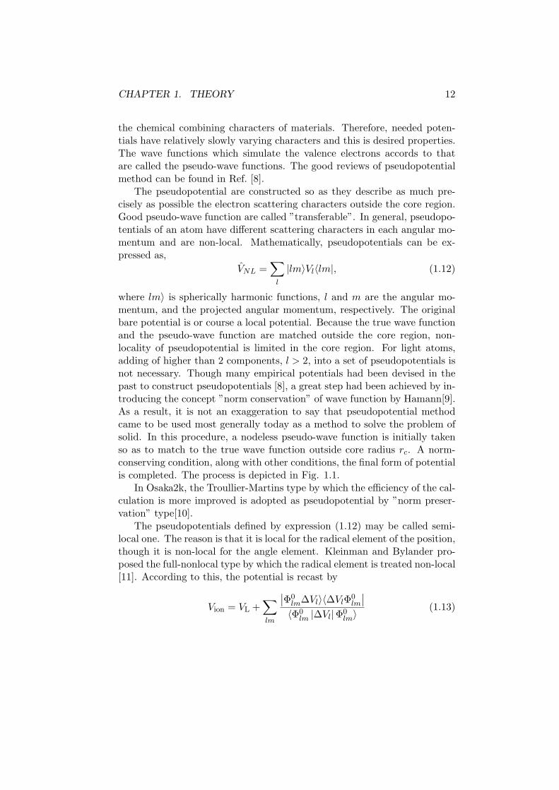
where lm〉 is spherically harmonic functions, l and m are the angular mo-mentum, and the projected angular momentum, respectively. The originalbare potential is or course a local potential. Because the true wave functionand the pseudo-wave function are matched outside the core region, non-locality of pseudopotential is limited in the core region. For light atoms,adding of higher than 2 components, l > 2, into a set of pseudopotentials isnot necessary. Though many empirical potentials had been devised in thepast to construct pseudopotentials [8], a great step had been achieved by in-troducing the concept ”norm conservation” of wave function by Hamann[9].As a result, it is not an exaggeration to say that pseudopotential methodcame to be used most generally today as a method to solve the problem ofsolid. In this procedure, a nodeless pseudo-wave function is initially takenso as to match to the true wave function outside core radius rc. A norm-conserving condition, along with other conditions, the final form of potentialis completed. The process is depicted in Fig. 1.1.
In Osaka2k, the Troullier-Martins type by which the efficiency of the cal-culation is more improved is adopted as pseudopotential by ”norm preser-vation” type[10].
The pseudopotentials defined by expression (1.12) may be called semi-local one. The reason is that it is local for the radical element of the position,though it is non-local for the angle element. Kleinman and Bylander pro-posed the full-nonlocal type by which the radical element is treated non-local[11]. According to this, the potential is recast by
Vion = VL +∑
lm
∣∣Φ0lm∆Vl〉〈∆VlΦ
0lm
∣∣〈Φ0
lm |∆Vl|Φ0lm〉
(1.13)

CHAPTER 1. THEORY 13
rc
pseudo wavefunction
↑
↑true wavefunction
pseudo potential
↑
↑ Z/r
Figure 1.1: Outline of pseudopotential A true wave function (solid
curve) can be replaced with a pseudo-wave function (dashed curve).
Wave function and potential of all electrons are the same each other in
the chemically important area outside the core radius rc
where Φ0lm is the pseudo-wave function of the atom when the pseudopotential
is constructed. ∆Vl is obtained by
∆Vl = Vl,NL − VL. (1.14)
Giving nonlocal potential in this way, the calculation of non-local part of thepotential is greatly accelerated. Further benefit is obtained in calculationof operating of nonlocal potential onto wave functions if the arbitrariness ofVL is utilized.

CHAPTER 1. THEORY 14
1.4 Plane-wave expansion
There are about ∼ 1023 atoms in real crystals. It is intractable to solvedirectly the KS equation for the system with such degrees of freedom, whichis virtually infinite dimension. For such a system, it is convenient to use theartificial mathematical tool of Born-von Karman’s boundary condition andBloch theorem[13].
Not only plane-wave method, but almost all the calculation methods ofsolids undergo a benefit of the periodical boundary condition. For problemsof surface of solids, defects, and even for completely disordered solids, wecan study these materials by assuming large super cells, which are of courseartifacts though.
A mathematical model of a crystal is constructed from three basic trans-lational vectors in the real space:
t = n1R1 + n2R2 + n3R3, (1.15)
where n1, n2, n3 are arbitrary integers. The lattice constructed from theprimitive translational vectors is called Bravais lattice. Crystals are ex-pressed by combining a Bravais lattice and the basis, which is composed ofall the atoms in the primitive unit cell.
The reciprocal lattice space is defined for a lattice in the real space. Thebasic translational vectors of the reciprocal lattice space are defined so as tosatisfy
Ri · Gj = 2πδij , (1.16)
where i and j take an integer value from 1 to 3. Now, we have G1 as
G1 = 2πR2 × R3
R1 · (R2 × R3). (1.17)
G2,G3 can obtained by cyclic change the indeces. The lattice vectors of thereciprocal lattice (reciprocal vector) can be expressed as
G = n1G1 + n2G2 + n3G3 (1.18)
where n1, n2, n3 are arbitrary integers.Reciprocal vectors are used for Fourier transformed expression of arbi-
trary functions with periodicity. When f(r) is a smooth function of R,we can expand it by
f(r) =∑
G
AGeiG·r, (1.19)

CHAPTER 1. THEORY 15
Under the periodic boundary condition, the electron state is specifiedby the wave vector k and band index n. The wave function has a form ofproduct of a plane wave exp(ik · r) and a periodic function uk(r) with thelattice periodicity,2
Ψkn(r) = exp(ik · r)uk(r). (1.20)
This is what Bloch theorem states, which reduce greatly a problem of solidsfrom nearly infinity to the orders of the number of atoms in the unit cell.
There are many kinds of band calculations, but these are different merelyat a point of the ways to express wave functions, i.e., basis functions, exceptthe cellar method.
Because uk(r) in Eq. (1.20) is a periodical function of the lattice, it canbe expanded by the reciprocal lattice vectors according to Eq. (1.19), andthen is expressed by,
Ψkn(r) =∑
G
ck+Gei(k+G)·r. (1.21)
Because plane waves satisfy the Bloch’s condition by construction, theyprovide a good expression as valence electrons in crystal, which are extendedover the crystal. Various quantities of the ground states can be expressedneatly by this expansion. On the other hand, a disadvantage of this methodis slow convergence (see Ref. [8]).
The total energy Eq. (1.3) is written by plane waves, [14]
Etot =∑
i,G
|cki+G|2(ki + G)2
+1
2
∑
G
ρ∗(G)VH(G) +3
4
∑
G
ρ∗(G)Vxc(G)
+∑
G
ρ∗(G)S∗(G)VL(G) +∑
i,l,G,G′
c∗ki+Gcki+G′
×S(G′ − G)V NLl (ki + G,ki + G′) + Eion(Rn), (1.22)
where S(G) is the structure factor. In addition, the Hellmann-Feynmanforce and stress, etc, can be evaluated also easily by this plane wave expan-sion, which will be seen later.
2Alternatively, the exponential form can be taken as exp(−ik · r). In this program, tokeep consistency with TSPACE, we decided to the definition of Eq. (1.20)
CHAPTER 1. THEORY 16
The last term of Eq. (1.22) is the so-called Ewald term, which corre-sponds to the direct Coulomb interaction between ions
Eion(Rn) =e2
2
∑
κ,κ′
ZκZκ′γκ,κ′ , (1.23)
where κ is the atom index in the lattice cell, and γκ,κ′ is given by
γκ,κ′ =∑
l′
′erfc
(η
∣∣R(
l′
κ′ κ
)∣∣)
R(
l′
κ′ κ
)
+4π
Ωc
∑
G 6=0
′ 1
G2exp
[−
(G
2η
)2]
exp [iG · (xκ − xκ′)]
− 2η√π
δκ,κ′ − π
2η2Ωc. (1.23a)
Here, κ 6= κ′ is understood in the primed summation. η is so taken as thesummation over the real space and that on the reciprocal space in Eq. (1.23a)becomes good convergent. (see. Ref. [15], p. 385)
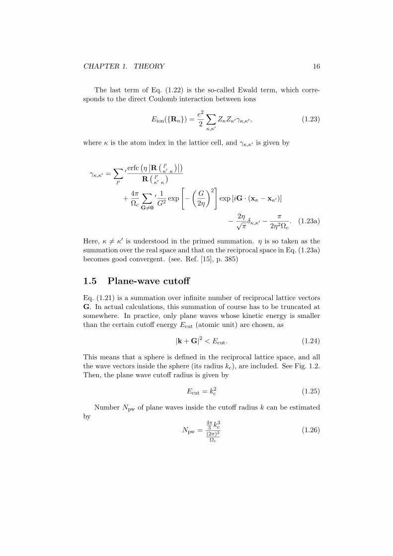
1.5 Plane-wave cutoff
Eq. (1.21) is a summation over infinite number of reciprocal lattice vectorsG. In actual calculations, this summation of course has to be truncated atsomewhere. In practice, only plane waves whose kinetic energy is smallerthan the certain cutoff energy Ecut (atomic unit) are chosen, as
|k + G|2 < Ecut. (1.24)
This means that a sphere is defined in the reciprocal lattice space, and allthe wave vectors inside the sphere (its radius kc), are included. See Fig. 1.2.Then, the plane wave cutoff radius is given by
Ecut = k2c (1.25)
Number Npw of plane waves inside the cutoff radius k can be estimatedby
Npw =4π3 k3
c
(2π)3
Ωc
(1.26)

CHAPTER 1. THEORY 17
kc
k i
kc
FFT Box
NGDIM(a) (b)
Wavefunctionsphere
Charge-densitysphere
Figure 1.2: (a) Expanding plane waves for ki. (b) relationships betweenplane wave sphere, the charge density sphere, and FFT box.
where Ωc is the volume of the primitive lattice cell.Number Npw of plane waves needed for good convergence depends on
the atom type in the primitive unit cell. In general, the systems containingelements of 1st row in the periodic table need a cutoff energy larger thansystem containing only elements of 2nd or 3rd rows.
1.6 k-space summation
In the calculation of the total energy and forces, taking an average of oper-ator Q which acts on the Kohn-Sham wave functions is often needed.
According to Bloch’s theorem, the average over all the wave functions iscalculated by
Q =Ωc
(2π)3
∫
BZQkd3k, (1.27)
where Qk is given byQk = 〈Ψkn|Q|Ψkn〉. (1.28)
For example, in the case in which Q is Kohn-Sham Hamiltonian, Qkn is theeigenvalue of Kohn-Sham equation, and Q is the average value of the bandenergy of n-th band.

CHAPTER 1. THEORY 18
In the numerical calculation of Eq. (1.27), the integral can be replaced bythe summation of finite points in k-space, and it usually takes a lot of time.However, with choosing wisely enough a set of special points, we could obtainas accurate as by using much more k points. This is called the special pointsampling method. In our program, the method by Monkhorst and Pack [16]is used as the standard special point sampling method. The mesh of k pointsis created by three integers of N1, N2, and N3. These integers determine thedensity of k points in a primitive unit cell of reciprocal lattice. A generalpoint of the mesh is given by
krst = u1rG1 + u2sG2 + u3tG3 (1.29)
uip =2p − Ni − 1
2Ni, (1.30)
where p takes a value from 1 to Ni. This mesh makes N1N2N3 pieces ofk points in the Brillouin zone. Therefore, the integral of (1.27) is replacedwith the summation of discrete k points.
Q =1
N1N2N3
∑
rst
Qkrst(1.31)
Some k points are occasionally points on symmetry line or planes. If somek points are connected each other by symmetry, it is enough to solve theKohn-Sham equation at only one point of the group of symmetry-connectedpoints (stars). By using symmetry, computation time can be greatly saved.In Osaka2k, the number of k points is decreased as much as possible byproperties of crystal symmetry and time-reversal symmetry.
The quality of the special-point sampling is accessed by the cutoff vectorsof the real space. Periodical functions of the reciprocal space like Qk can beexpressed by the Fourier series in the real space
Qk =∑
R
BReik·R, (1.32)
where BR are expansion coefficients. B0 is the average of Qkn over theBrillouin zone. Usually, the Fourier coefficient BR decreases rapidly withincreasing |R|. Inserting (1.32) into (1.31), we get
Q = B0 +∑
R 6=0
BRφR, (1.33)
where φR can be written by
φR =1
N1N2N3
∑
rst
eikrst·R. (1.33a)
CHAPTER 1. THEORY 19
The summation of φR over R 6= 0 can be regarded as an error of Q for aparticular set rst of sampling points. By classifying R through |R|, i.e.,shell structure of R, the summation of Eq. (1.33) can be grouped by shells,as
ith shell∑
R
φR. (1.33b)
As the shell sum vanishes to further extent, the qualify of the samplingpoints becomes better.
1.7 Conjugate gradient method in Kohn-Sham func-tional
Next, it is necessary to solve Eq. (1.3). A traditional method to solvethis is to diagonalize Eq. (1.5) self-consistently so that the output chargedensity and input charge density become to match. In this method, theoutput charge density is returned to as the input of the next step, by mixingit with the old input charge density. How set the mixing rate is subtleproblem. Especially when the size of a crystal becomes large, adjustment ofthe mixing rate is indeed a tough business. The conjugate-gradient methodin Kohn-Sham functional is an excellent method to solve this difficulty. Wewill explain in detail below.
Based on the arguments so far made, to seek the ground states of a crystalis equivalent to a problem of minimizing the total energy EKS(ck+G,n)by varying plane-wave expansion coefficients ck+G,n of all the occupiedbands.
It is known that conjugate-gradient method is an efficient mathematicaltechnique to find the minimum point of multi-dimensional functions f(x).Especially, when f(x) can be approximated by quadric form,
f(x) =1
2x · A · x − b · x + c, (1.34)
and when A is positive-definitive, one can always find the minimum point,at least in principle.
Because a gradient of function f(x) at x is given by
−∇f(x) = b − A · x, (1.35)
the minimum point x satisfies the following linear equation
A · x = b. (1.36)
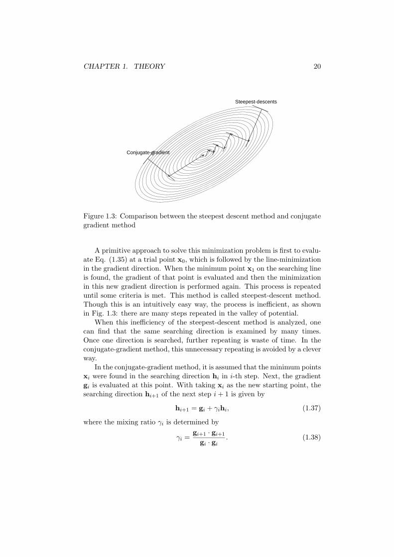
CHAPTER 1. THEORY 20
Conjugate-gradient
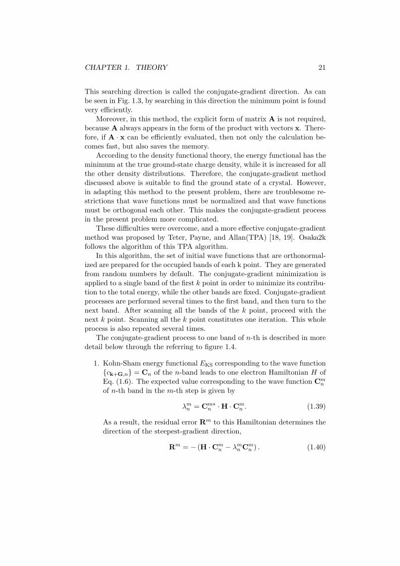
Steepest-descents
Figure 1.3: Comparison between the steepest descent method and conjugategradient method
A primitive approach to solve this minimization problem is first to evalu-ate Eq. (1.35) at a trial point x0, which is followed by the line-minimizationin the gradient direction. When the minimum point x1 on the searching lineis found, the gradient of that point is evaluated and then the minimizationin this new gradient direction is performed again. This process is repeateduntil some criteria is met. This method is called steepest-descent method.Though this is an intuitively easy way, the process is inefficient, as shownin Fig. 1.3: there are many steps repeated in the valley of potential.
When this inefficiency of the steepest-descent method is analyzed, onecan find that the same searching direction is examined by many times.Once one direction is searched, further repeating is waste of time. In theconjugate-gradient method, this unnecessary repeating is avoided by a cleverway.
In the conjugate-gradient method, it is assumed that the minimum pointsxi were found in the searching direction hi in i-th step. Next, the gradientgi is evaluated at this point. With taking xi as the new starting point, thesearching direction hi+1 of the next step i + 1 is given by
hi+1 = gi + γihi, (1.37)
where the mixing ratio γi is determined by
γi =gi+1 · gi+1
gi · gi. (1.38)
CHAPTER 1. THEORY 21
This searching direction is called the conjugate-gradient direction. As canbe seen in Fig. 1.3, by searching in this direction the minimum point is foundvery efficiently.
Moreover, in this method, the explicit form of matrix A is not required,because A always appears in the form of the product with vectors x. There-fore, if A · x can be efficiently evaluated, then not only the calculation be-comes fast, but also saves the memory.
According to the density functional theory, the energy functional has theminimum at the true ground-state charge density, while it is increased for allthe other density distributions. Therefore, the conjugate-gradient methoddiscussed above is suitable to find the ground state of a crystal. However,in adapting this method to the present problem, there are troublesome re-strictions that wave functions must be normalized and that wave functionsmust be orthogonal each other. This makes the conjugate-gradient processin the present problem more complicated.
These difficulties were overcome, and a more effective conjugate-gradientmethod was proposed by Teter, Payne, and Allan(TPA) [18, 19]. Osaka2kfollows the algorithm of this TPA algorithm.
In this algorithm, the set of initial wave functions that are orthonormal-ized are prepared for the occupied bands of each k point. They are generatedfrom random numbers by default. The conjugate-gradient minimization isapplied to a single band of the first k point in order to minimize its contribu-tion to the total energy, while the other bands are fixed. Conjugate-gradientprocesses are performed several times to the first band, and then turn to thenext band. After scanning all the bands of the k point, proceed with thenext k point. Scanning all the k point constitutes one iteration. This wholeprocess is also repeated several times.
The conjugate-gradient process to one band of n-th is described in moredetail below through the referring to figure 1.4.
1. Kohn-Sham energy functional EKS corresponding to the wave functionck+G,n = Cn of the n-band leads to one electron Hamiltonian H ofEq. (1.6). The expected value corresponding to the wave function Cm
n
of n-th band in the m-th step is given by
λmn = Cm∗
n · H · Cmn . (1.39)
As a result, the residual error Rm to this Hamiltonian determines thedirection of the steepest-gradient direction,
Rm = − (H · Cmn − λm
n Cmn ) . (1.40)

CHAPTER 1. THEORY 22
TRIAL WAVE FUNCTION FOR BAND
Calculate steepest-descent vector
Orthogonalize to all bands
Precondition vector
Orthogonalize to all bands
Determine conjugate direction
Orthogonalize to present band andnormalize
Calculate Kohn-Sham energy oftrial value of
Calculate value of
that minimizesKohn-Sham energy functional
CONSTRUCT NEW TRIAL WAVE FUNCTION
REPEATN TIMES
orUNTIL
CONVERGED
Figure 1.4: Flow diagram of the direct minimization method
The mean square of this Rm is called the residual error ξm of wavefunctions.
2. This residual error vector Rm is corrected so as to orthogonal to otherbands of the k point:
R′m = Rm −∑
r 6=n
(Cr · Rm)Cr. (1.41)
3. To accelerate the convergence, this corrected residual error vector R′m
is preprocessed (preconditioning). That is, a suitable weighting matrixK is multiplied in order for all the diagonal elements of R′m to be ofthe same order of magnitude,
R′′m = R′m · K. (1.42)
CHAPTER 1. THEORY 23
In practice, the matrix K is so constructed as a diagonal matrix, whosediagonal element is given by the inverse of the corresponding elementof R′m roughly.
4. Modifying R′′m again so that it is orthogonal to all the bands includingitself.
Gm = R′′m −∑
r 6=n
(Cr · R′′m
)Cr −
(Cm
n · R′′m)Cm
n . (1.43)
5. Using this Gm, the conjugate gradient is obtained. That is,
Fm = Gm − γmFm−1 (1.44)
is given for the conjugate gradient. The mixing ratio γm can be ob-tained from Gm according to Eq. (1.38). γ0 can be set to be 0 as theinitial condition.
6. Fm is orthonormalized with the present band again. We denote it byDm. By this way, the line minimization problem in the direction Dm
becomes in turn the minimization problem of the total energy EKS(θ)as a function of θ.
Cm+1n = Cm
n cos θ + Dm sin θ. (1.45)
7. Since EKS(θ) is a function of the density, and the density is propor-tional to the square of the wave function, if EKS(θ) can be approxi-mated to be linear in the density, EKS(θ) may be expressed by
EKS(θ) = const + A cos 2θ + B sin 2θ. (1.46)
Because there are three unknown numbers in Eq. (1.46), three equa-tions are necessary. Value EKS(0) with θ = 0 has already been evalu-ated, and its derivative is also obtained easily as,
∂EKS
∂θ
∣∣∣∣∣θ=0
= 2fnRe(Dm∗ · H · Cmn ) (1.47)
Because H ·Cmn has already been evaluated, Eq. (1.47) is obtained by
only taking the scalar product of vectors. B in Eq. (1.46) is half avalue given by Eq. (1.47).

CHAPTER 1. THEORY 24
8. The remaining variable can be obtained either by evaluating EKS(θ)with θ1 6= 0 or by calculating the second derivative of EKS(θ) at θ = 0.We will use the later way here. By this way, A is given by A =(1/4)∂2EKS/∂θ2. Then, θmin minimizing Eq. (1.46) is determined by
θmin = −1
2tan−1
−
∂EKS
∂θ
∣∣∣θ=0
12
∂2EKS
∂θ2
∣∣∣θ=0
(1.48)
1.8 Fast Fourier transform
An important part of calculation in the conjugate-gradient method is tooperate the Kohn-Sham Hamiltonian on the wave functions. In the program,this step is carried out by using the Fast Fourier Transform (FFT). Osaka2kutilizes the fact that the kinetic energy is local in the reciprocal space, andthat local potential is diagonal in the real space.
Given the number of basis function Npw, calculation of the kinetic en-ergy from in the reciprocal space needs arithmetic operations O(Npw) inEq. (1.22). On the other hand, because the local potential is a matrix of thesize Npw, the calculation in the reciprocal lattice space needs operations ofO(N2
pw). This operation can be accelerated by rewriting with a real spacerepresentation,
∑
G′
VL(G − G′)ck+G′,n =1
Ωc
∫e−iG·rVL(r)
∑
G′
eiG′·rck+G′,nd3r. (1.49)
From Eqs. (1.20, 1.21), we see that summing ckd + Gd gives
ukn(r) =∑
G′
eiG′·rck+G′,n. (1.50)
Therefore, the evaluation of Eq. (1.49) is:
1. To convert the wave function ck+G,n expanded in the reciprocal spaceinto the representation ukn(r) in the real space.
2. To take the product of ukn(r) and VL(r) in the real space.
3. To convert the result to its representation in the reciprocal space.
Though this three-step calculation seems more involved than the direct prod-uct of V ·C in the reciprocal space, it actually is superior in terms of com-putation speed.

CHAPTER 1. THEORY 25
Because the operation of 2 is actually a diagonal sum in the real space,the number of floating-point arithmetic is only O(Npw). Operations of 1 and3 needs only the number of floating-point arithmetic of order O(Npw log(Npw)),when FFT is used. The number of overall operation is therefore still orderof O(Npw log(Npw)). This technique was devised by Car and Parrinello[20]and has become widespread.
It may be worth to notice the region on which FFT is performed. Thewave functions are expressed in a spherical region with the radius kc, inwhich Npw plane waves are involved, as shown in Fig. 1.2 (a). On theother hand, in order to express the charge density faithfully for varyingwave functions, we must take a sphere of the twice radius in the reciprocalspace. See the figure (b). As a result, the rectangular region on which FFTis performed is the length of4kc. The mesh in the reciprocal space is almostthe same as that in the real space. According to Eq. (1.26), the number ofmesh points in the real space, NFFT is given by
NFFT∼= 16Npw (1.51)
1.9 Hellmann-Faynman forces and stresses
Hellmann-Faynman theorem enables us to calculate atomic forces and stresseseasily.
In a material, a force exerted on an atom whose position is given by RI
is given by energy derivative with respect to RI
FI = −dEtot
dRI
= − d
dRI
〈Ψ|H|Ψ〉 (1.52)
By this definition, in order to estimate atomic forces, the total energy mustbe evaluated at several (at least two) points of RI .
Hellmann Faynman theorem reduces this task considerably,[21] In vertueof this theorem, Eq. (1.52) can be recast as
FI = −〈Ψ|∂V (R)∂RI
|Ψ〉 (1.53)
At a glance, difference between Eq. (1.52 and (1.53) might seem notsignificant. But, the difference is definite. In Eq. (1.52), wave functionΨ has implicitly dependence on atom positions. Once atom positions arechanged, Ψ must be recalculated. On the other hand, in Eq. (1.53), Ψ isthe wave function at the equilibrium positions. Schrodinger equation is once

CHAPTER 1. THEORY 26
solved, and only once is enough. What you have to do is merely integrationof wave function over new external potential. The latter task is much easierthan performing another SCF calculation.
Evaluation of forces and stresses can be done straightforwardly in plane-wave expansion. Because the basis functions are fixed in the real space,application of Hellmann-Feyman theorem is simple and yield no correctionterm, such as Purley correction.
For concrete expressions, see [14] for atom forces, and se [22, 23] forstresses.3
Information of atom force is utilized for optimization of atom positions,Similarly, information of stresses is utilized for cell optimization.
It should be noted that in general convergence speed about force andstress is much slower than that of the energy. The total energy is a variablewith respect to the change in wave functions. This means that the varia-tion of the total energy around the equilibrium state is second order in thevariation of wave function. On the other hand, the variation of force is onlythe first order.
3In Ref. [23], in Eq. (2), the sign appearing in front of kinetic energy is mistyped as−.

Chapter 2
Load Map
2.1 Overview
A electronic-structure calculation package of ”Osaka2002” based on pseu-dopotential method is actually a set of several program codes. The relation-ship between them is shown in Fig. 2.1.
In brief, given a crystal, which is constructed by cryst, prepare atomicpotentials of constituting the crystal by atom, carry out self-consistent field(SCF) calculation by pwm. inip does preparation to pass some parametersto pwm.
The core of Osaka2002 is pwm. Once SCF calculation is completed, wehave several choices to proceed further. Among them are optimization ofthe crystal, phonon calculation, molecular dynamics simulations.
If you need to know details of electronic spectra, band and DOS calcula-tions can be obtained by pwbcd. pwbcd has an option to display wavefunc-tions in the real space.
atom is a program to generate pseudopotentials, and is independent ofthe rest of the package Osaka2k.
Throughout all the calculations, full use of crystal symmetry was made.This is accomplished thanks to a library TSPACE.
2.2 Preparation
directory structure
After downloading the source codes, expand in a suitable directory. On ex-pand, you will see four directories, as shown in Fig. 2.2. Users should create
27

CHAPTER 2. LOAD MAP 28
(inip)
Preparation
(pwm)
(pwbcd)
DOS calc.
Band calc.
WFs disp.
(cryst)Create a crystalGenerate atom pseudopotentials
(atom)
Self-Consistent Calculation
constant T
constant Tp
Molecular Dynamic Simulation
Atom optimization
Cell optimization
under pressures
Phonon calculation
Figure 2.1: Overiew of Osaka2002
a directory /bin, in which executable codes are stored. For users conve-nience, we add a directory /drivers, which is not shown in the figure. Inthis directory, machine-dependent files and Makefile are stored. Users shouldadd a working directory /data, in which you will carry out calculation.
All the source codes are put in directory /fsrcs, along with Makefile.These are copied into directory /bin, and are compiled to create executablecodes. These executable codes will be copied or linked into a working direc-tory which contains a crystal data you want to calculate, such as /sidat inthe figure.
Directory /input contains template files for input.
The current version of Osaka2002 is featured by being reusable; once

CHAPTER 2. LOAD MAP 29
fsrcs/
bin/
Makefile
pwminipcryst
all the sourc codes
ppot/ si.pot si.pwfc_.pot
generatorwycoffrel/spn/
psmap.datmat.dpatom/ atomk.f
atom.dat
/atomscript...
data/
input/
sidat/grdat/...
si.xtl
...
...
copy and make
linkcopypwm.parainip.para ...
nom/
com/
Figure 2.2: Directory structure of Osaka2002
executable codes are compiled, there is no need to recompile them when acrystal or calculation conditions are changed. In a previous version writtenby old Fortran, many calculational parameter should be given before com-pilation, and thereby recompilation was needed whenever these parametersor crystals were changed. Only one exception is TSPACE, because this waswritten at so old age.
compile
First of all, find Makefile, drivs.f90 suitable to your machine in /drivers,put these in /fsrcs. Then, edit /drivs.f90 as described latter. When youlike to get benefits of the maximum performance of your machine, furtherarrangements, such as in fft util.f90, may be needed. Some of techniques

CHAPTER 2. LOAD MAP 30
are described in ”Installation Manual of Osaka2002”.
Copy Makefile in /bin, type
% make prep
Then, all the needed files are copied in /bin.
All the executable codes are created by Makefile. For inip,
% make inip
For pwm,
% make
After comilation, unnecessary files will be deleted by commands
% make clean
or
% make clobber
For pwbcd, which carrys out band, DOS calculations along with others,
% make pwbcd
Atom potentials are created in /patom, the data files should be restoredin directory /ppot.
2.2.1 machine dependence
After copied necessary files in /fsrcs, modify these in order to meet your mi-chine. In /drivers, machine-dependent codes such as Makefile, drivs.f90,are put in according to specific machines. Suitable ones should be moved to/fsrcs, and add modification.
In drivs.f90, find a subroutine potdir, and edit a part
CHARACTER(LEN=15) :: datadir = ’/home/user/ppot’
CHAPTER 2. LOAD MAP 31
in order to meet your environment. This is the directory in which atomicpotentials are restored. Note that LEN is exactly matched to the length ofdatadir. It is our observation that, even though datadir is correct, thelength is often wrong, so that it failed to find the potential files.
pwm uses a mathematical library lapack. Describe the method to linkthis library in Makefile, according to your system construction. TSPACE
is troublesome, because this is written by old style Fortran. Some of tipsof handling TSPACE is described in Appendix of ”Installation Manual ofOsaka2002”
For TSPACE usersTSPACE enclosed in this package is basically the same as thatof Ref. [24]. However, in order to make more flexible to treatvariety of materials, some parameters are written in a separatefile TSPARAM and the file is included at the compilation time.Therefore, TSPACE in this package must be used.
2.3 Input parameters
Every program in the package requires input data, as usual. These data arecommonly written in a file named as *.para. The format of these files willbe described in order to appear. Here, notices applied commonly in thesefiles are described.
One of problems which came to be clear on the course of the programdevelopment, is that, at every time program revision is made, input param-eters are subjected to change. In case this is often happened, to rewrite themanual only due to minor changes is indeed troublesome for both of thewriter and users. In many cases, actually such a minor change of parameterdoes not relate to the uses of average users. On the basis of this painfulexperiences, we decided that a standard file *.para explicitly keeps onlyfew parameters, which are frequently used. Others are added when needed.The way to add these parameters is to use option input.
2.3.1 Input options
Options are to be added according to user’s special needs. Because theseextended features are continuously progressed as the program is developed, itis not suitable to describe this kind of text. These things belongs to details

CHAPTER 2. LOAD MAP 32
of revision, so that these are described separately in a form of TechnicalReport Series associated with Osaka2002.
Here, we describe only general rules in adding options, which are commonin every *.para file.
First of all, keep distinction of upper and lower cases, i.e., options arecase sensitive.
After describing general input parameters, make one empty line, thentype
OPTION BEGIN
specify each option followed byOPTION END
During these description, do not insert blank lines.
There are two types of options.
1. toggle variablesfermi broadening ON
Type the name of variable, and put one (and only one) space, followdby ON/OFF.
2. value variablespressure=
1.5
Type the name of variable, followed by= without any space. Then,after carriage return, its value is typed after at least one space. Whena real number is entered, type for example 300. even when the valueis just 300.
The available options are subjected to change as the program code isdeveloped, refer Technical Report Series, or a source file auxinp.f90. Indirectory input, there is a file opts list, which lists all the implementedoptions.
This completes file preparation. Now, we can proceed to creation of atomicpotentials in the next chapter

Chapter 3
Atomic pseudopotentials
One feature of contemporary pseudopotential method is that a part of cre-ating potential can be separated from the rest of bulk electronic structurecalculation. Currently, there are several program codes to generate pseu-dopotentials. Package Osaka2k uses one of such program, atom, which isdeveloped by Troullier and Martins. Hence, we cannot owe responsibilityfor this program, even though we will explain sometimes principles underly-ing this code. Although utility of this program is really wide, we restrictedour concerns to those related to pwm.
The source code is atomk.f in directory /patom.1。To create atom, type
f77 atomk.f -o atom
After creating an executable atom, generate atom pseudopotentials neededone by one 2
3.1 input file
First, edit an input file atom.dat. The format is as follows,The meaning of each line is as follows
1st line type of calculation (itype) and title(ititle).As types of calculation,itype=
1The original code is atom.f. Only change made in atomk.f is output format in orderto meet the input of pwm
2Although the code is well developed, there is still some machine dependence. Theseare referred to ”Installation manual”
33

CHAPTER 3. ATOMIC PSEUDOPOTENTIALS 34
Table 3.1: Format of atom.dat
itype ititle
ikerknameat icorr + isppznuc zsh rsh rmax aa bbncore nval
n l zo↓ zo↑ evd...
rcs rcp rcd rcf cfac rcfac
• ae: all-electron calculation
• pg: generation of pseudopotential
• pe: generation of pseudopotential with core correction withrespect to the exchange-correlation term
• ph: generation of pseudopotential with core correction includingthe Hartree term
• pt: test of pseudopotential
• pm: test of pseudopotential and modification of valence elec-trons
2nd line kind of pseudopotential (ikerk)ikerk=
• tm2 Improved Troullier and Martins
• bhs Bachelet, Mamann, Schuter
• oth generate data file
• van Vanderbilt
• tbk Troullier and Martins
• yes Kerker
• no Hamann, Schluter, Chiang
3rd line atom name(nameat) and options(icorr + ispp).nameat is just atom name. icorr+ispp is consisted of three characters.The first two corresponds to icorr and gives the type of electron-correlation functional. Those available areicorr=

CHAPTER 3. ATOMIC PSEUDOPOTENTIALS 35
• ca Ceperly-Alder (Perdew-Zunger parameterization)
• xa Xα method
• wi Wigner interporation scheme
• hl Hedin-Lundqvist
• gl Gunnarson-Lundqvist-Wilkins
• bh von Barth-Hedin
The third character corresponds to ispp and gives a selectionispp=
r relativistic calculation
s spin polarization
t none
4th line charge number of nucleus (znuc), charge of inner core (zsh), coreradius (rsh), maximum radius(rmax), parameters of radial mesh(aa,bb).
5th line number of core orbitals(ncore) and number of valence orbitals(nval)
after 5th line occupation of the valence orbitals specified by n and l(zo).The orbital energy as option input (evd).
last line cutoff radii for generating pseudooptentials(rc).Further parameters are added when core correction is needed (cfacand rcfac).
Atomic orbitals are specified by three quantun numbers, i.e., the princi-pal quantum number n, angular-momentum l, and its azimuthal componentm, even when spin freedom can be ignored. In atom (and most of otherprograms of this kind), spherical potentials are assumed. This treatmentmeans, for example, when there is only one electron available among px,py, and pz orbitals, each orbital is occupied equally by 1/3 electron. Thiskeeps the dimensionality of problem within only one dimension. Otherwise,the problem would become essentially three dimensional one, for which so-lutions become much more complicatd. Therefore, third quantum numberm is ignored.
In the following, we explain how to specify these parameters, taking Sias example.

CHAPTER 3. ATOMIC PSEUDOPOTENTIALS 36
pg Silicon
tm2
n=Si c=ca
0.0 0.0 0.0 0.0 0.0 0.0
3 2
3 0 2.00 0.00
3 1 2.00 0.00
2.13 2.57 1.50 1.50
The first line gives the code of calculation kind, name of atom, while thesecond gives the kind of pseudopotential. For now, we write as
pg generation of pseudopotential
tm2 Improved Troullier and Martins
The third line is written as shown. The forth line is ignored. Leave italone.
The fifth line gives the numbers of core and valence orbitals, which arespecified by two quantum numbers n and l. In the present example of Si, theneutral atom is configured by (1s)2(2s)2(2p)6(3s)2(3p)2. This means thatthere are three core orbitals; 1s, 2s, and 2p, while two 3s aned 3p orbitalsare included as the valence orbitals.
Next, occupation numbers are followed. In each line, one valence orbitalis described by specifying n, l, the number of occupation of down-spin andup-spin. In the present case, spin freedom is ignored, the occupation numberof only down-spin is used. For Si, two electrons are occupied for 3s and twoare occupied 3p orbital.
The last line gives the cutoff radii for generating pseudopotentials inorder of s, p, d, f orbitals. Values are given in atomic unit.
3.2 execution
We explain the basic usage of atom. Advanced usage of it should be referredin related Technical Reports.
1 All electron calculation First, all electron calculations including allcore orbitals must be performed. Set pg as the type of calculation, 3
3All electron calculation is originally performed by setting ae. But, in the processof generating pseudopotentials, all electron calculation is performed before creation ofpseudopotential.

CHAPTER 3. ATOMIC PSEUDOPOTENTIALS 37
At this moment, you may do not wary about the values of the cutoffradii. Putting a data file atom.dat in the same directory as atomk, executeatomk.
2 Read an output file atom.out In an output file atom.out, results ofall-electron calculation is written. The eigen-energy of all the orbitals arelisted, along with information about the shape of orbitals along in the radialaxis. Users are encouraged to plot orbitals. For doing so, fort.11 can beused.
In file atom.out, after
radial grid parameters
the characteristics of each orbital in the radial direction is listed, as
n = 2 l = 0 s = .0
a extr .634 -1.373
r extr .057 .458
r zero .153
r 90/99 % .903 1.348
This describes the features of 2s orbital. This orbital has two extreme andone zero point other than the origin. The position of zeros are given by r
zero in Bohr units. r extr indicates the position of extreme. Users shouldcheck if the obtained orbitals behave as expected.
Next, determine the cutoff radii for generating pseudopotentials, by see-ing the shape of valence orbitals. There is to a large extent arbitrariness inchoosing the cutoff radius rc. This arbitrariness causes beginners confusion(not only beginners but experts too). At the first trial, it may be taken tobe 1.1 ∼ 1.6 times larger than the position of the most outer extremum,by rule of thumb. It can be set to be inside of the most outer exremum,as far as it still is outside of the most outer zero point. In general, as rc isset to be larger, the obtained potential becomes soft and consequently goodconvergence is achieved. A bad news is degradation of transferability.
One feature of the Troullier-Martins type is that rc can be larger thanothers such as Bachelet et. al. [12]. The cutoff radii are written in the lastline of atom.dat.
3 Generating pseudopotentials After deleting all the previous outputfiles, again execute atom. Then, all the needed files are created. The pseu-

CHAPTER 3. ATOMIC PSEUDOPOTENTIALS 38
dopotential and pseudo-wave functions are written in fort.10. Users areagain encouraged to see these as graphics output.
In fort.10, wavefunctions and potentials are listed in order s, p, ... Eachdata are listed as two column data; the first is the radial position and thesecond is the value of wavefunction/potential. At the first, the number ofmesh points appears.
The pseudopotential data as output is the bare-ion one, which the elec-tronic contribution has been removed, and the wavefunction u(r) is normal-ized as it were. This means that it holds
∫ ∞
0|u(r)|2dr = 1 (3.1)
but not∫· · · rdr.
4 Give the names for data files Finally, take binary files pseudo.dat01and fort.13 among various output files. The former is the potential data,while the latter is the pseudo-wave function data. These files are actuallyused in the following calculations. Rename these and saved in directory/ppot/nom. The file name of potential should be (atom name).pot, andthe name of wavefunction should be (atom name).pwf. Atom name is givenby two characters. In the present case, these are si.pot and si.pwf, re-spectively. In case of C, underscore should be followed, such as c .pot andc .pot. The name characters should be written by lowercase. It should benoted that *.pot and *.pwf files are usable only on the current platform,since these data are written binary format. When platform is changed, thenpotential and wavefunction data should be recalculated on that platform.
5 Repeat if necessary The above process is repeated for used atoms.
To what extent can we take as the valence electron?
As studying various materials, you will find it problem to determine whichelectron is counted as the valence electron and which is counted as thecore electron. For light elements, such as Si, this seems definite. But,for 4f elements and heavy elements, such distinction becomes difficult. Inaddition, we are further embarrassed with questions as to what configurationof electrons should be used as the reference state when pseudopotentials areconstructed.
All of these problems are essential problems in the pseudopotential method.As a guide, we supply input templates for all the elements in /patom/atomscripts.

CHAPTER 3. ATOMIC PSEUDOPOTENTIALS 39
However, this is by no means the best set, nor even correct. When you beginto suspect these supplied data, and when try to change the input data tosee how the result is influenced, then this is a sign that you are qualified asa real and active researcher in this field. You will search the literature anddiscuss a problem to other researchers.
Chapter 4
Construction of crystals
4.1 Input of crystal data
Crystals are described by the lattice of the unit cell and the atoms con-stituting the lattice. The primitive unit cell is the minimum lattice whichpreserving the translational symmetry. However, more large cells called asconventional unit cell are often used due to practical reasons.
In the primitive unit cell, the unit translational vectors are expressedby a set of R1, R2, and R3, while in the conventional unit cell the unittranslational vectors are expressed by a set of a, b, and c.
When referring the coordinate (h, k, l) without any notice, we cannotsay which of hR1 + kR2 + lR3 or ha + kb + lc is meant by. The formeris said as the expression in the primitive base, while the expression in theconventional base. Correspondingly, the reciprocal lattice is expressed byG1, G2, and G3 in the primitive base, while a∗, b∗, c∗ in the conventionalbase.
Usually in the crystallographic literature, a crystal is described in theconventional base, by using three lengths, (a b c), of the lattice vectors andits three angles (α, β, γ), where α means the angle between b and c axes,and so on.
In cryst, by using a, b, c, α, β, and γ, the lattice vectors are translatedin the cartesian coordinated, as
a = ax
b = b(cos γx + sin γy)
c = c(cos βx + ry +√
1 − cos2 β − r2z) (4.1)
40
CHAPTER 4. CONSTRUCTION OF CRYSTALS 41
where r is given by
r = (cos α − cos β cos γ)/ sin γ.
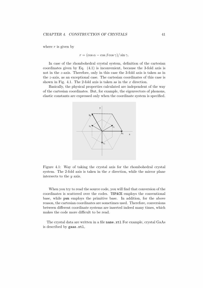
In case of the rhombohedral crystal system, definition of the cartesiancoordinates given by Eq. (4.1) is inconvenient, because the 3-fold axis isnot in the z-axis. Therefore, only in this case the 3-fold axis is taken as inthe z-axis, as an exceptional case. The cartesian coordinates of this case isshown in Fig. 4.1. The 2-fold axis is taken as in the x direction.
Basically, the physical properties calculated are independent of the wayof the cartesian coordinates. But, for example, the eigenvectors of phonons,elastic constants are expressed only when the coordinate system is specified.
t1t2
t3
h1
h2
x
y
Figure 4.1: Way of taking the crystal axis for the rhombohedral crystalsystem. The 2-fold axis is taken in the x direction, while the mirror planeintersects to the y axis.
When you try to read the source code, you will find that conversion of thecoordinates is scattered over the codes. TSPACE employs the conventionalbase, while pwm employs the primitive base. In addition, for the abovereason, the cartesian coordinates are sometimes used. Therefore, conversionsbetween different coordinate systems are inserted indeed many times, whichmakes the code more difficult to be read.
The crystal data are written in a file name.xtl For example, crystal GaAsis described by gaas.xtl,
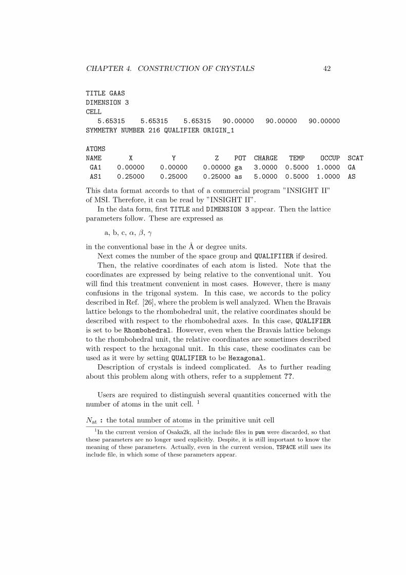
CHAPTER 4. CONSTRUCTION OF CRYSTALS 42
TITLE GAAS
DIMENSION 3
CELL
5.65315 5.65315 5.65315 90.00000 90.00000 90.00000
SYMMETRY NUMBER 216 QUALIFIER ORIGIN_1
ATOMS
NAME X Y Z POT CHARGE TEMP OCCUP SCAT
GA1 0.00000 0.00000 0.00000 ga 3.0000 0.5000 1.0000 GA
AS1 0.25000 0.25000 0.25000 as 5.0000 0.5000 1.0000 AS
This data format accords to that of a commercial program ”INSIGHT II”of MSI. Therefore, it can be read by ”INSIGHT II”.
In the data form, first TITLE and DIMENSION 3 appear. Then the latticeparameters follow. These are expressed as
a, b, c, α, β, γ
in the conventional base in the A or degree units.Next comes the number of the space group and QUALIFIIER if desired.Then, the relative coordinates of each atom is listed. Note that the
coordinates are expressed by being relative to the conventional unit. Youwill find this treatment convenient in most cases. However, there is manyconfusions in the trigonal system. In this case, we accords to the policydescribed in Ref. [26], where the problem is well analyzed. When the Bravaislattice belongs to the rhombohedral unit, the relative coordinates should bedescribed with respect to the rhombohedral axes. In this case, QUALIFIERis set to be Rhombohedral. However, even when the Bravais lattice belongsto the rhombohedral unit, the relative coordinates are sometimes describedwith respect to the hexagonal unit. In this case, these coodinates can beused as it were by setting QUALIFIER to be Hexagonal.
Description of crystals is indeed complicated. As to further readingabout this problem along with others, refer to a supplement ??.
Users are required to distinguish several quantities concerned with thenumber of atoms in the unit cell. 1
Nat : the total number of atoms in the primitive unit cell1In the current version of Osaka2k, all the include files in pwm were discarded, so that
these parameters are no longer used explicitly. Despite, it is still important to know themeaning of these parameters. Actually, even in the current version, TSPACE still uses itsinclude file, in which some of these parameters appear.

CHAPTER 4. CONSTRUCTION OF CRYSTALS 43
Nspe: the number of chemical elements constituting the crystal
Nka : the number of distinct atom sites (irreducible sites), which are notconnected by symmetry
Distinction between Nspe and Nka is important. In the former classification,all the atoms are counted as one, if these atoms are the same chemicalelement. On the other hand, in the latter classification, even when theatoms are the same chemical element, they are counted as different kinds ifthey cannot be transformed by crystal symmetry.
For example, in graphite crystal, these parameters are
Nspe = 1, Nka = 2, Nat = 4
In a file *.xtl, it is not necessary to list all the atom coordinates inthe primitive unit cell. Listing only prototype atoms at the irreducible sitessuffices. Hence, only number Nka of atoms appear in the list. Other atomsare created by symmetry operations in cryst. In the package or home page,files many crystals are available, so that you can exercise how to describecrystals.
In a line, NAME comes first. This name is arbitrary. Next, three relativecoordinates come, followed by the name of potential. This name of potentialis the one by which the correct potential data file is searched, so that it mustbe the same as the name of the potential. For example, for Si atom, youshould type si. For C, you shoud type one character c followed by onespace, as ct.
The remaining data are not used, accordingly you can omit them. 2
Description of QUALIFIER accords to ”International Tables for Crystal-lography” (ITC) [25]. These available descriptions are
ORIGIN 1 or ORIGIN 2
For the trigonal system,
RHOMBOHEDRAL or HEXAGONAL
For low-symmetry crytals,
UNIQUE b or UNIQUE c
2In a previous version, the next data of valence number was required. Now, this is notnecessary. These data are read in from /ppot/com/psmap.dat

CHAPTER 4. CONSTRUCTION OF CRYSTALS 44
and
UNIQUE b,CELL 1, 2 or 3
Due to the restriction of TSPACE, for base-center lattices, only C center isacceptable. Hence, when the data are described in another center, it shouldbe rewritten on C center, and specify CELL n as QUALIFIER
4.2 Execution of cryst
Next, execute cryst by using data *.xtl. As an output, you will get *.prim.After this point, all the calculation refers *.prim as the crystal data, but not*.xtl. It may useful to remember that all the data in the calculation after*.prim are expressed in the atomic units. Only in output, some conventionalunits are sometimes used. In this case, explicit units will be given. Hence,if specific units are not given, the atomic units are assumed.
First place a file si.xtl in a working directory /sidat, then executecryst. You are asked to answer
input the crystal name with a period at the end.
> si.
You should type as above, including a period at the last.
The output file si.prim should be checked.Title and date appear, and the conventional unit cell, primitive unit cell,
the reciprocal lattice vectors in the cartesian coordinates are followed, as
TITLE GAAS
date: Fri Jan 5 17:56:20 2001
DIMENSION 3
LATTICE PARAMETERS (A,B,C,CA,CB,CC) in a.u.
10.6829045 10.6829045 10.6829045
0.0000000 0.0000000 0.0000000
Space group
216 Td2 F-43m ORIGIN_1
IL NG NC
2 24 1 ORI
The conventional vectors
10.6829045 0.0000000 0.0000000
0.0000000 10.6829045 0.0000000
0.0000000 0.0000000 10.6829045
The primitive vectors

CHAPTER 4. CONSTRUCTION OF CRYSTALS 45
0.0000000 5.3414522 5.3414522
5.3414522 0.0000000 5.3414522
5.3414522 5.3414522 0.0000000
The primitive reciprocal vectors without 2Pi
-0.0936075 0.0936075 0.0936075
0.0936075 -0.0936075 0.0936075
0.0936075 0.0936075 -0.0936075
IL, NG, and NC, which are parameters of TSPACE, are the type of lattice,the order of crystallographic point group, and the number of choices of theorigin.
By using the space-group number, the crystal structure is constructed.It is important to check the output crystal structure. Nspe and all the chem-ical elements in the crystal are listed. Then, Nka comes, and the Wyckoffpositions of each sites are follows
Number of atom species
2
No Name Zat Zval
1 ga 31 3
2 as 33 5
KIND OF ATOMS
2
Wycoff Positions
ATM ( x, y, z) Nos Wycf Code
1 ( 0.00000, 0.00000, 0.00000) 1/ 1 4a 0 0/1 0 0/1 0 0/1
2 ( 0.25000, 0.25000, 0.25000) 3/ 1 4c 0 1/4 0 1/4 0 1/4
NUMBER OF ATOMS
2
L.L. AND U.U. VALENCE ELEMENT
1 1 3.0000 1 ga
2 2 5.0000 2 as
POSITIONS RELATIVE TO A UNIT CONVENTIONAL CELL SPECIES SYM(IG)
1 0.0000000 0.0000000 0.0000000 1 ga 1
2 0.2500000 0.2500000 0.2500000 2 as 1
After Wyckoff positions, Nat appears. After subtitle L.L. AND U.U., allNat atoms are classified as Nka cites, each line lists the range of those atomsbelonging to an irreducible site. One line also contains the valence number,so that you should check it. Finally, relative coordinates of every atoms arelisted.
Note
CHAPTER 4. CONSTRUCTION OF CRYSTALS 46
On the outset, we should confess that quality of cyrst is lessthan other components of Osaka2k, in a sense of described be-low. cyrst attempts to determine Wyckoff positions by givencoordinates and the space group information. Because 230 kindsof space groups are so complicated, this attempt in the presentcode does not guarantee to always success. For more details, re-fer to a supplement [?]. When it failed, cryst assigns the failedcite to a general point. Accordingly, user should take care of thisassignment. If the assignment is wrong, you are required to fixmanually. to a supplement [?].
Notations of Wyckoff positions accords to those of ITC. Its positionalcode accords to those ofTSPACE. This is composed of three components. Ineach component is composed of an integer and a fraction number. Theinteger part means that 1, 2, and 3 means the relative coordinates x, y,and z, respectively, while 0 means just 0. When sign - are preceded to x,then negative value of x is meant. The fraction number are added to theinteger part. For instance, 1 0/1 2 1/4 -2 1/4 means a coordinate(x, y + 1
4 , −y + 14).
4.3 Control parameters
So far, there is no case where users are required to modify parameters. Formost cases, the default values of TSPARAM will suffice. But, if you want tocalculate a large-size crystal, these default values may be insufficient. Inthis case, you are required to modify these by yourself.
TSPARAM are directory read and used in TSPACE, but these parametersare transformed explicitly or implicitly to other programs, such as cryst,inip, and pwm, and hence you should be care of setting these parameters.
PARAMETER (LMNATM=50,LMNKAT=20)
PARAMETER (MAXNPW=4854)
LMNATM specifies the upper limit for Nat in the unit cell, and LMNKAT specifiesthe upper limit for Nka. Therefore, it is recommended to take larger valuesthan those actually used.
MAXNPW specifies the upper limit of the number of planewaves. But, thenumber of planewaves here is different one in pwm. Hence, you can set avalue smaller than that used in pwm.

CHAPTER 4. CONSTRUCTION OF CRYSTALS 47
4.4 Graphics display of crystal structure
At this level, users must want to check correctness of crystal data by graph-ics, as well as numerics. Few people if not could imagine a crystal figure bynumerics only, but most cannot do so without help of graphics.
There are many tools (commercial or public domain) to display crystalstructures. Osaka2k offers a set of Mathematica notebooks to analyze re-sults. Among them, CrsytAnal.nb analyzes the data *.prim. In order todisplay crystal structures, you are required only few input parameters, suchas file name, in this Mathematica nootbook. Mathematica is very flexible,and I like this in data analysis. But, if you want to analyze further, forexample, to calculate bond lengths or angles, you may need to knowledgefor Mathematica.
Figure 4.2: GaAs crystal. The red line indicates the primitive unit cell.
You will feel that commercial programs are easier to use than Mathe-matica nootbook. On the other hand, if you want to do further analysis,you may find after all that efforts as much as to understand Mathematicanootbook is required.
Although I do not here describe how to use Mathematica nootbook,those people who know the basics of Mathematica would not be difficult tounderstand that. Appendix A helps those people to use.
In Fig. 4.2, an example of crystal structure drawn by CrystAnal.nb is

CHAPTER 4. CONSTRUCTION OF CRYSTALS 48
shown.

Chapter 5
Ground states of electronicstructures (I)
5.1 inip
Before proceeding to pwm, some preparations are needed. This is done byinip. 1
One important purpose of inip is to expand the basis set of plane waves,given cutoff radius kc in the reciprocal space. Count the number of planewaves Npw, and the cut the FFT box out. The relationships of the size ofkc to NGDIM and NG3, which determine the FFT box, are shown in Fig. 1.2.The length of one edge of FFT box is 2*NGDIM+1 in the k space, and theone in the real space NADIM=2*NGDIM.
Another purpose of inip is to determine k sampling point on the sum-mation over the Brillouin zone, which is discribed in the next section.
A input file inip.para looks like as follows,
Input file name (priod is needed at the end)
si.
Parameters about k points
Cutoff k radius (AMAX) given by lattice index without 2Pi
3.1
way to give sampling points (0:given manually, 1:calc)
1In the previous version, the chief purpose of inip is estimation of the size of matricesappearing in pwm, in order to write them in a include file. In the current version, all theinclude files have been discarded, and accordingly such roles of inip is unnecessary. But,other things which are done by inip are still needed, and hence inip is left as beingseparated from pwm
49

CHAPTER 5. GROUND STATES OF ELECTRONIC STRUCTURES (I)50
pwm
inip
inip.para
pwm.para
pwm_si.outpwm_si.sumpwm_si.etotpwm_si.ekspwm_si.frcpwm_si.rhopwm_si.wfn(pwm_si.vrs)pwm_si.inp
pwm_si.wfn
/ppot/ data
si.potgenerator ...
inip_si.out
inip_si.kpt
inip_si.rmesh
inip_si.inp
si.prim
si.xtl
cryst
Figure 5.1: relationships among various files of pwm
1
number of k-sampling points
2
potential type (spin, NLCC, relativistic)
0 0 0
In the following, the meaning of these parameters are explained.First the name of crystal comes with a period, which is followed by the
cutoff radius for the plane wave expansion
• the cutoff radius of the plane waves (AMAX)the cutoff radius for the plane wave expansion kc is given in the unitsof minimum value of the primitive reciprocal vectors gmin.
• Way of giving k sampling1: automtic calculation, 0: manual input

CHAPTER 5. GROUND STATES OF ELECTRONIC STRUCTURES (I)51
• number of segments of k sampling (NKDIV)number of segments of k sampling when automatic calculation
• options for pseudopotentiallist of potential options. Three options are spin, core correction, andrelativistic effect. 1 indicates ON, while 0 indicates OFF. These op-tions are the same as those for pseudopotential-generation programatom, and thereby both must be the same.
Any information of potential type used pwm is inherited from the aboveparameters in inip. and accordingly no specification appears in pwm.para.
5.1.1 specail k-point sampling
There are several ways to giving k sampling points, as shown in the following.
(i) Automatic calculation(isotropic and uniform sampling ≡ defualt)
When automatic calculation is chosen, k points are determined accordingto the method of Monkhorst-Park as described in Sec 1.6.[16] In default, thefirst zone is divided by M , indexing from (−M + 1)/2M to (M − 1)/2M ineach of three principal direction in 2π/a units.
For example, when M = 1, only Γ is sampled. WhenM = 2, thereare 8 points, i.e., (1/4, 1/4, 1/4) and ones changed with every sign. In areal crystal, further reduction of k points is achieved, because of crystalsymmetry and time-reversal symmetry.
In Fig. 5.2, a feature of Monkhorst-Park is compared to that of beginner.A beginner would take first the center point, next the zone boundary points,and further proceed by taking the midpoint. On the other hand, Monkhorst-Park method avoids the zone center point and the boundary points as far aspossible. This method gives better accuracy than that of beginners on thesame computational task.
Even numbers for M is recommended, except when M = 1.This value of M is given for input NKDIV. The determined sampling
points and the total number is written out in an output file inip *.inp, as
nkpts
2
Sampling point in p
LD -1 -1 -1/ 4 WTK= 0.250000
XY 1 -1 -1/ 4 WTK= 0.750000

CHAPTER 5. GROUND STATES OF ELECTRONIC STRUCTURES (I)52
amateure?
0 1/2-1/2
Ndiv
1
2
4
8
Monkhorst-Pack mesh
0 1/2-1/2
1/4
1/8
1/16
Figure 5.2: Comparison of k-point mesh between the method of Monkhorst-Park method and of amatua. In Monkhorst-Park method, the zone-centerand zone-boundary points are avoided as far as possible.
In the above example, for an input M = 2, the final number of samplingpoints, nkpt, only two. Remember the initial number of created k pointsis 8. Symmetry reduced greatly nkpt. You can see that these points are(−1/4,−1/4,−1/4) and (1/4,−1/4,−1/4) in the primitive base, and thesampling wights are 1/4 and 3/4, respectively.
(ii) Automatic calculation (anisotropic sampling)For crystals which are significantly anisotropic, such as super lattices,
the above isotropic sampling is inefficient. In this case, anisotropic mesh isdesirable. For doing so, optional parameters are available.
In inip.para, at the end of basic parameters, place one blank line, whichis followed by
OPTION BEGIN
anisotrop_ksample=
1 1 4 4
OPTION END
By declaring anisotrop ksample=, the uniform division NKDIV previouslygiven is made no effect. In the next line, the first three numbers mean the
CHAPTER 5. GROUND STATES OF ELECTRONIC STRUCTURES (I)53
segment numbers for the three primitive vectors g1, g2, and g3, respectively.The last one means the least common multiple (LCM) of first three integers.Since inip does not check correctness of this LCM, users should be carefulfor giving this number.
(iii) Manual inputAutomatic calculation for giving k sampling point is convenient. On the
other hand, there are cases in which a more flexible way to give samplingpoints is needed. In this case, user can specify sampling points manually.A user should determine sampling points by himself. The way of giving thepoints determined is as follows,
The portion from 6 to 9 lines in the above list for inip.para is replacedwith
way to give sampling points (0:given manually, 1:calc)
0
number of k-sampling points
4
KB(3), ICB
-1 -1 -1 4
1 0 0 4
0 1 0 4
0 0 1 4
This example gives four points (1/4, 1/4, 1/4) and (1/4, 0, 0) and its cycli-cally changed points.
For the hexagonal system, other sampling method such as Chadi-Cohenalgorithm [30] may be useful. In this case, the sampling points are given inthis way.
When the number mesh points is small, a way of k sampling is critical.For example, when the total energies are compared among various polymor-phic modifications, equivalent sampling method is important. Super latticesand polytypes of SiC are good examples [31].
In any method, it is desirable to estimate how used sampling is good.To do so, use of Eq. (1.33b) is made. In the section of inip *.out,
=====> Final report for k-point sampling <=====
you will find a list as
Quality of sampling by 2-points...
list only nonzero shells up to 41 shells
Sh No shell sum

CHAPTER 5. GROUND STATES OF ELECTRONIC STRUCTURES (I)54
8 ( -1.00000, 0.00000)
15 ( 1.00000, 0.00000)
23 ( -1.00000, 0.00000)
26 ( -1.00000, 0.00000)
28 ( 1.00000, 0.00000)
32 ( -1.00000, 0.00000)
36 ( 1.00000, 0.00000)
38 ( 1.00000, 0.00000)
This is a list of only those shell sums in Eq. (??) which gives no zero. Inthe example shows that the shell sum vanishes up to 7th shell.
5.1.2 Cutoff radius of planewaves
Another important parameter is the cutoff radius (AMAX) for plane waveexpansion. The dimensionless input parameter AMAX is related to the cutoffradius kc in the k space by
kc = AMAX ∗ gmin, (5.1)
where gmin is the minimum length of the three primitive reciprocal vectors.The cutoff energy Ecut is given by Eq. (1.25) in the atomic units.
For each sampling point ki, all the plane waves G which satisfy Eq.(1.24) are taken as the basis set. Accordingly, the number of plane wavesNpw differs slightly from point to point.
In an output file inip *.out, you will find an example as
=====> Final report for k-point sampling <=====
For cutoff energy in Ry = 4.959185
NHDIM = 59
NGDIM = 4
nkpts= 2
Name: LD -1 -1 -1/ 4 NSTR= 8 WTK= 0.25000 NPW= 55 INV= 6
Name: XY 1 -1 -1/ 4 NSTR= 24 WTK= 0.75000 NPW= 50 INV=18
Sum over WTK 1.000000
From this, you see that point (−1/4,−1/4,−1/4) and (1/4,−1/4,−1/4)have different Npw, 55 and 50, respectively. The basis set of these points arestored in an output file inip *.kpt. inip determines the dimension of thearray of basis set (NHDIM) as the maximum of these Npw’s, i.e., 59.
Along with NHDIM, parameters used for pwm are summarized in the lastsection of inip *.out, as
Passed parameters
NEPC 8 NEDIM 4

CHAPTER 5. GROUND STATES OF ELECTRONIC STRUCTURES (I)55
NKPTS 2 NHDIM 59
NGDIM 4
Then, ...
LIN SEG NGLIN 9 NADIM 8
VOL SEG NG3 729 NA3 512
As another role of inip creates a list of real-space points, which are con-nected by the crystal symmetry. This data is stored in a file inip *.rmesh.When there is no symmetry, i.e., the space group is P1, this file is notcreated.

CHAPTER 5. GROUND STATES OF ELECTRONIC STRUCTURES (I)56
5.2 pwm
The core program of Osaka2k is pwm. This program calculates the electronicground states for a given crystal. This is achieved by self-consistent energyminimization for the energy functional as described in Sec. 1.7.
After creating an executable code pwm as described in Sec. 2.2, make acopy or link pwm into your working directory.
5.2.1 SCF calculation
Input parameters for pwm is written in pwm.para. There are a couple ofparameters, which control calculations. As described earlier, we ceased topack all the input parameters in the standard format of pwm.para. Instead,rarely used parameters are written by optional input, when need occurs.
A typical form of pwm.para looks like as follows,
Input file name
si.prim
Job (0:SCF Calc. 1:Atom optimize 2:Cell optimize 3:Phonon 4:MDS)
0
atom movement (0: OFF, 1: ON valid only when cell optimization)
0
number of iteration for electrons (maxIter0wfn)
15
conjugate-gradient paths (npath)
5
wftol
1.0D-11
ftol
8.0D-5
etol
1.0D-12
iread (previous WFs)
0
imoni,irhout,iwfout
0 1 1
Resume atom relaxation
0
max number of iterations for atoms (maxIter0atom)
4
Resume cell relaxation
0
max number of iterations for cell (maxIter0cell)

CHAPTER 5. GROUND STATES OF ELECTRONIC STRUCTURES (I)57
2
In the following, meaning of each parameters are explained.
xtl.name name of crystalJobNo Job type
0 : SCF calculation (default)1 : optimization of atom positions2 : optimization of unit cell4 : MDS
atomMove0ctrl atom relaxation 0 : no (default) 1 : domaxIter0wfn the maximum number of iterations for energy
minimization process with respect wave functionsnpath0wfn iteration number of conjugate-gradient paths for a bandwftol tolerance of wavefunction error (Ry2)ftol tolerance of HF forces (Ry/aB
2)etol tolerance of energy (Ry)iread wfn selection of initial wave functions 0: random data (default)imoni0ctrl monitoring 0 : OFF (default)irhout output of charge density 1: ON (default)iwfout output of wave functions 1: ON (default)atomMove resume resume of atom relaxation 0 : OFF (default)maxIter0atom the maximum iterations for atom relaxationcellMove resume resume of cell relaxation 0 : OFF (default)maxIter0cell the maximum iterations for cell relaxation
The most important parameters are those of convergent criteria. Asdescribed in Sec. 1.7, the electronic ground state can be found by itera-tive minimization of the total energy. As the smallest iteration loop, theminimization process by the conjugate-gradient method is applied to oneband at a ki point. For a band, the conjugate-gradient path is repeatedby npath0wfn. Then, this process is repeated over the all bands of nbandat a ki point. After completing this at ki, proceed to the next kj point.After repeating over all the k sampling points, one iteration in the mostouter loop is completed. This outer loop will be repeated by maxIter0wfn,if convergence criteria are not satisfied.
Among these parameters, the most frequently changed may be maxIter0wfn.This value may be chosen to be about 5. SCF calculation will stop, whenthe iteration of the outer loop exceeds maxIter0wfn, or when the error of

CHAPTER 5. GROUND STATES OF ELECTRONIC STRUCTURES (I)58
wave functions becomes less that wftol, or when energy variation from theprevious step becomes less that etol
If you intend to achieve SCF calculation of electronic ground state only,JobNo is set to be 0. In this case, all the remaining parameters afteratomMove resume are ignored.
For a given crystal, at the first time of calculation, set iread wfn=0. Inthis case, the initial wave functions are created by random data.
As output control, there are three options to output files, monitering(imoni0ctrl), charge density (irhout), wave functions (iwout). Usually,set imoni0ctrl=0. Only for debugging, this will be changed. When treat-ing a large crystal, and if you do not need further calculation than SCFcalculation for the fixed crystal, then you can save memory not to outputwave function file by setting iwout = 0. It is noted that, to save memory,wavefunction data is written in binary file. Hence, this file is usable only onthe working machine.
On completing the above preparation, you can run pwm. When shortcalculation, directory type
% pwm
After launching pwm, the process of calculation is flowing out on the display.When long calculation, it should be put on as a background job, by
% pwm>stdout &
Because pwm prints out some output directly on the display, the above redi-rection for output is needed, otherwise causes output error. When the jobis put on a queue system, keep instructions of the system.
It is important to estimate the calculation time for a given crystal. Asa guide, we include benchmark tests in a directory bncmrk. This was donefor a crystal containing 8 Si atoms. Various platforms were examined. Youcan acquaint some idea about how long calculation is taken.
5.2.2 Interpretation
On completing calculation, pwm outputs various files as shown in Fig. 5.1.
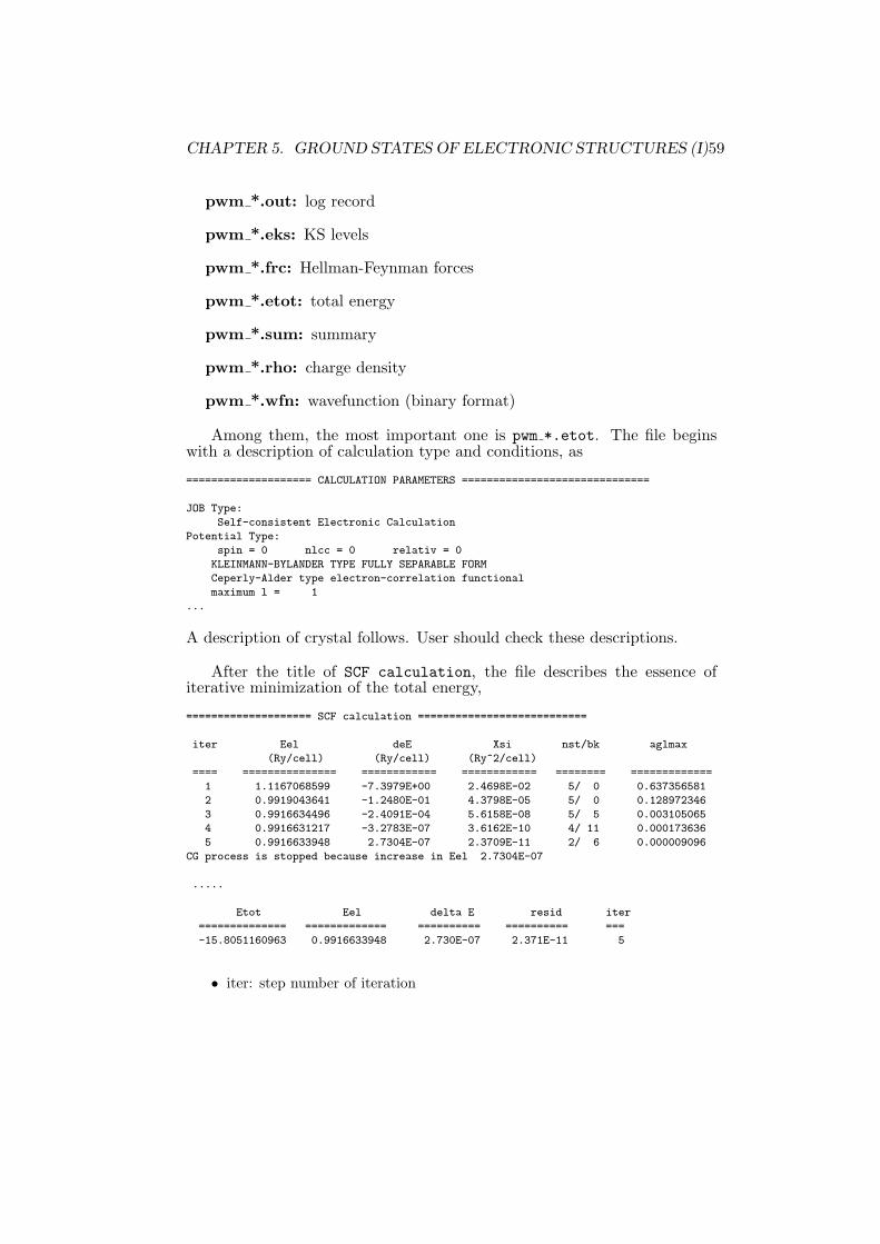
CHAPTER 5. GROUND STATES OF ELECTRONIC STRUCTURES (I)59
pwm *.out: log record
pwm *.eks: KS levels
pwm *.frc: Hellman-Feynman forces
pwm *.etot: total energy
pwm *.sum: summary
pwm *.rho: charge density
pwm *.wfn: wavefunction (binary format)
Among them, the most important one is pwm *.etot. The file beginswith a description of calculation type and conditions, as
==================== CALCULATION PARAMETERS ==============================
JOB Type:
Self-consistent Electronic Calculation
Potential Type:
spin = 0 nlcc = 0 relativ = 0
KLEINMANN-BYLANDER TYPE FULLY SEPARABLE FORM
Ceperly-Alder type electron-correlation functional
maximum l = 1
...
A description of crystal follows. User should check these descriptions.
After the title of SCF calculation, the file describes the essence ofiterative minimization of the total energy,
==================== SCF calculation ===========================
iter Eel deE Xsi nst/bk aglmax
(Ry/cell) (Ry/cell) (Ry^2/cell)
==== =============== ============ ============ ======== =============
1 1.1167068599 -7.3979E+00 2.4698E-02 5/ 0 0.637356581
2 0.9919043641 -1.2480E-01 4.3798E-05 5/ 0 0.128972346
3 0.9916634496 -2.4091E-04 5.6158E-08 5/ 5 0.003105065
4 0.9916631217 -3.2783E-07 3.6162E-10 4/ 11 0.000173636
5 0.9916633948 2.7304E-07 2.3709E-11 2/ 6 0.000009096
CG process is stopped because increase in Eel 2.7304E-07
.....
Etot Eel delta E resid iter
============== ============= ========== ========== ===
-15.8051160963 0.9916633948 2.730E-07 2.371E-11 5
• iter: step number of iteration

CHAPTER 5. GROUND STATES OF ELECTRONIC STRUCTURES (I)60
• Eel: the energy of electrons Eel
• ∆E: change in Eel from the previous step
• ξ: residual error in wavefunction, Eq. (1.40)
• the number of paths actually carried out/ the number of back path: usuallythe former number is equal to the set value npath. But, at sometime, theconjugate-gradient paths are stopped before reaching the npath step, becauseof satisfaction of other criteria of convergence. At sometime, the minimiza-tion process fails by some reasons. The electron energy may be increased. Ifthis happens, then the conjugate-gradient process for this band is stopped,and the number of such an event is counted as the number of back path.
• θ: the maximum value of mixing angles of all the bands, θ, in Eq. (1.45)
As shown in the example, as the process proceeds, Eel is decreased,accordingly the absolute of ∆E, ξ, and θ are also decreased. The processis stopped at step 5, because|∆E| < etol. Then, the total energy Etot isprinted at the last by adding the electrostatic energy of ions Eewald to theconverged electron energy Eel.
Next, decomposition of the total energy Etot is listed as
component of Etot
kin 5.97858894
hart 1.08391474
exc -4.78172988
loc -1.80253465
nonloc 0.51342418
ewald -16.79677949
----------------------------
total -15.80511616
This decomposition is given by Eq. (1.22). From this analysis, which con-tribution dominates the total energy may be investigated. However, thisway of decomposition is somewhat arbitrary or is based on mathematicalconvenience. Hence, users should remain that to place too much physicalmeaning on them is dangerous.
For example, although the ion-ion electrostatic interaction energy, i.e.,Ewald term Eq. (1.23) seems to be most definite, it cannot be so clearlyseparated from other terms. In Ref. [23], it is shown that the Ewald termis decreased, when a Si crystal is compressed. Because all the ions in Sicrystal have +4 charge, it will be expected that the electrostatic energyshould be increased as the inter-atomic distance is decreased. This seeminglyunexpected result is a consequence of the fact that even Ewald term is not

CHAPTER 5. GROUND STATES OF ELECTRONIC STRUCTURES (I)61
independent of other interaction terms such as ion-electron interaction in aform of Eq. 1.22. [27]
At the last, stress components are listed as
total stress (Ry/Bohr^3)
S(1,1)= -2.24759E-05 S(2,3)= 3.17724E-10
S(2,2)= -2.24759E-05 S(3,1)= 2.52820E-10
S(3,3)= -2.24756E-05 S(1,2)= -1.10795E-10
By evaluating stresses for a given strain, we can calculate elastic constants.The total stress also can be decomposed as for the total energy. This is donein pwm *.strs. However, some cautions are needed in the interpretation asfor the decomposition of the total energy.
For example, the first term of the total energy in Eq. (1.22) represents thekinetic energy. The corresponding component of the total stress is given by
∑
i,G
|cki+G|2(ki + G)α(ki + G)β (5.2)
in Eq. (2) of Ref. [23]. This correspondence is clear. But, if you interpret the above
expression 5.2 as indicating the change exactly in the kinetic energy component in
the total energy given by Eq. (1.22), it would be wrong. I means that the two is
numerically different. Hellmann-Faynman theorem guarantees that the total force
or stress are given by the change in the total energy if the true ground state is
found, but does not guarantees that each component of force or stress are given
by the change in the corresponding component of the total energy. This equalityholds only for the whole, but not for individual components.
Hellmann-Feynman forces for each atom are listed in pwm *.frc, as
HELLMANN-FEYNMAN FORCE (RY/BOHR)
ATOM X Y Z
ITER= 1
1 1 -0.230775E-08 -0.154249E-07 -0.573629E-07
1 2 0.637597E-07 0.428339E-07 0.299777E-07
These three components are expressed in the Cartesian coordinates, whichare those of used in constructing the crystal.
Accuracy of energyIn the above example, the electron energy Eel is well converged within ∆Eel <
10−8. User may be surprised to see that the value is in a good agreement with

CHAPTER 5. GROUND STATES OF ELECTRONIC STRUCTURES (I)62
each other among various platforms. This is a good news. Unfortunately, this doesnot mean that this accuracy gives smallness of the error in Eel from the true value.This merely indicates the numerical stability, even if the error from the true valueis large.
The error analysis of Eel is a complicated problem. This is an author’s sufferingnot to be able to provide the definite criteria as to which extent the magnitude oferror changes for given conditions.
Let us to evaluate errors in pwm from a viewpoint of general error analysisin numeric calculations. When referring errors in Eel, first it must be clarifiedwhat kinds of errors are involved. On input, errors (i) in input data can occur.During calculation, errors of (ii) rounding off and other inherent ones in digitalcomputations are unavoidable. Errors are also introduced (iii) by approximationsused in the calculation. All the errors are more or less amplified to yield the finalerror. This process is called error propagation, and is an important concept innumerical analysis, along with numerical stability.[29]
In the present analysis, forget the first kind of error, i.e., input error, such aserrors in a crystal structure, potentials, etc.
Let us estimate errors of kind (iii), especially, descretization errors in evaluatingthe total energy expressed by Eq. (1.22). For simplicity, only a term of ion-electron interaction is considered. It is given by an integration over the real space,∫
ρ(r)V (r)d3r. The integration is, of course, evaluated by summing over the finite
segmentations. When the integration∫ h
−hf(x)dx on the small finite range −h, h
is replaced merely by 2hf(0), the error is estimated by
1
6
f ′′
0
f0
h2 (5.3)
In the integration∫
ρ(r)V (r)d3r, the integrand is given by a product of thepotential and the charge density. Here, we simplify a problem by taking only apotential; ρ has merely an effect to smear the effective potential. For Si crystal, theintegration may be dominated by a contribution from the bond center, the value ofpotential and its second derivatives at the region are assumed in evaluation of Eq.(5.3), then they yield the coefficient of h2 to be ∼ 0.05. the width of mesh in thereal space h is given by a0/NADIM, where NADIM is the number of descritizationfor the lattice length a0 ∼ 7. When tt NADIM=16, the relative error becomes1 × 10−2. When NADIM=40, the relative error is barely improved by one order ofmagnitude.
By using a Si crystal, actual calculation is carried out by changing Ecut to seethe effect on the accuracy of Eel. In Table 5.1, the results are listed.
As shown in the Table, when NADIM=16, the value Eel has two digits of accuracyunder the decimal point. When NADIM=40, it has four digits of accuracy (Ry/cellunits). By considering the above assumption, the agreement between expectationand the result is good. According to Eq. (5.3), three times fine mesh is requiredto obtain the accuracy of Eel by one order of magnitude, since the relative error is
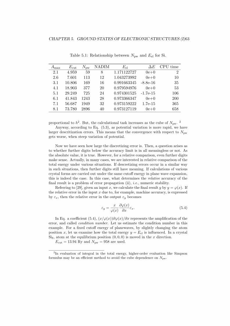
CHAPTER 5. GROUND STATES OF ELECTRONIC STRUCTURES (I)63
Table 5.1: Relationship between Npw and Eel for Si.
Amax Ecut Npw NADIM Eel ∆E CPU time
2.1 4.959 59 8 1.171122727 0e+0 22.6 7.601 113 12 1.043273992 0e+0 103.1 10.806 169 16 0.991663345 -8.8e-16 354.1 18.903 377 20 0.979594976 0e+0 535.1 29.249 725 24 0.974301525 -1.7e-15 1066.1 41.843 1243 28 0.973366347 0e+0 2007.1 56.687 1949 32 0.973159222 1.7e-15 3658.1 73.780 2896 40 0.973127119 0e+0 658
proportional to h2. But, the calculational task increases as the cube of Npw. 2
Anyway, according to Eq. (5.3), as potential variation is more rapid, we havelarger descritization errors. This means that the convergence with respect to Npw
gets worse, when steep variation of potential.
Now we have seen how large the discretizing error is. Then, a question arises asto whether further digits below the accuracy limit is in all meaningless or not. Asthe absolute value, it is true. However, for a relative comparison, even further digitsmake sense. Actually, in many cases, we are interested in relative comparison of thetotal energy under various situations. If descretizing errors occur in a similar wayin such situations, then further digits still have meaning. If calculations of variouscrystal forms are carried out under the same cutoff energy in plane wave expansion,this is indeed the case. In this case, what determines the relative accuracy of thefinal result is a problem of error propagation (ii), i.e., numeric stability.
Referring to [29], given an input x, we calculate the final result y by y = ϕ(x). Ifthe relative error in the input x due to, for example, machine accuracy, is expressedby εx, then the relative error in the output εy becomes
εy =x
ϕ(x)
∂ϕ(x)
∂xεx. (5.4)
In Eq. a coefficient (5.4), (x/ϕ(x))∂ϕ(x)/∂x represents the amplification of theerror, and called condition number. Let us estimate the condition number in thisexample. For a fixed cutoff energy of planewaves, by slightly changing the atomposition x, let us examine how the total energy y = Eel is influenced. In a crystalSi8, atom at the equilibrium position (0, 0, 0) is moved in the x direction.
Ecut = 13.94 Ry and Npw = 958 are used.
2In evaluation of integral in the total energy, higher-order evaluation like Simpsonformulus may be an efficient method to avoid the cube dependence on Npw.

CHAPTER 5. GROUND STATES OF ELECTRONIC STRUCTURES (I)64
10-1
10-2
10-3
10-4
10-5
10-6
10-7
10-8
10-9
10-10
10-11
10-12
10-16
10-15
10-14
10-13
10-12
10-11
10-10
10-9
10-8
10-7
10-6
10-5
10-4
ε u
εE
Figure 5.3: The relative error in the total energy, εE, of Si8 for the inputerror εu due to error of atom positions.
The result is shown in Fig. 5.3. From this figure, you can see that the conditionnumber is small enough over a wide range of error in u. This means numericalstability. By the relation of εE with respect to εu larger than 10−7, we can evaluatethat εE ∼ ε2
u. This reflects that the variation of potential from the equilibriumpotision is approximated by harmonic form.
In this way, we can see that because of good numeric stability of pwm, we can
compare the total energy exceeding two digits, if the same computational conditions
are used. The problem of energy accuracy is further discussed later (in Sec. 6.1.3).
5.2.3 Recalculation
If you find that one SCF calculation is not enough to achieve good conver-gence, then you can continue the calculation. In this case, the output data ofwavefunction is used as the input of the next calculation. User are required

CHAPTER 5. GROUND STATES OF ELECTRONIC STRUCTURES (I)65
to rename the output file pwm *.wfn as inip *.wfn, and set iread to be 1in pwm.para. Then, the next calculation will start with this wavefunctionas the initial state.
Estimation of various energiesHow can the total energy obtained in this way be interpreted? We have
evaluated the total energy by the pseudopotential method, i.e., Eq. (1.22).Therefore, only valence contribution is involved. Fortunately, most of chem-ical properties of solids are determined by valence electron solely. Manyinterested energies can be evaluated through evaluation of the total energyby pseudopotential method.
For example, the cohesive energy Ecoh(A) of element A can be estimatedby
Ecoh(A) = E(A(gas)) − E(A(sol)). (5.5)
The formation energy Eform(AmBn) of compound AmBn can be estimatedby
Eform(AmBn) = mE(A(sol)) + nE(B(sol)) − E(AmBn). (5.6)
When comparing the energy between solid and isolated atom, it is knownthat there is a problem regarding continuity of the exchange-correlation en-ergy. This is not a problem of pseudopotential approximation, but essentialproblem of DFT. There are many discussions in the literature, but here onlyone of early studies by pseudopotential is cited.[28].
5.2.4 Display of charge density
After you can complete pwm without trouble, the first quantity which you cansee is the total energy. But, the energy itself is relative quantity, in partic-ular, so in pseudopotential mathod. Even using the same pseudopotentialmethod, and even using the same pseudopotentials, you can see differentvalues between different implementations (different codes). It is almost im-possible to justify if the obtained value of total energy is reasonable, if yousee the total energy only. In most cases, to see the charge distribution is agood test for justifying the correctness of calculation.
The charge density in the real space is written out in file pwm *.rho. Theformat of pwm *.rho is that at the top the potential types (spin, NLCC,relativistic in input file inip.para) and the numbers of segmentations(NAX, NAY, NAZ) in the real space are described as
0 0 0
16 16 16
spin= -1

CHAPTER 5. GROUND STATES OF ELECTRONIC STRUCTURES (I)66
Figure 5.4: A surface of equi-density of charge for graphite
After spin identification, the charge density ρ(r) = ρ(i, j, k) is sequentiallywritten in order that i is taken as the most inner loop, while k is as the mostouter loop.
For visualization of charge density, a Mathematica notebookChgDnst.nbcan be used. As input, a crystal data *.prim and the charge density datapwm *.rho are used. As an example, three-dimensional plot of charge densityof graphite is shown in Fig. 5.4.
From the figure, you can see that honeycomb bonding is formed in a layer.In this way, three-dimensional display is useful for quick grasping how thecharge is distributed. Although appealing appearance, three-dimensionaldisplay has a disadvantage in less quantitative than two-dimensional contourmap of charge distribution. An example is shown in Fig. 5.5. There aretwo C atoms in a plane z = 1/4. The thick line indicates the boundary of

CHAPTER 5. GROUND STATES OF ELECTRONIC STRUCTURES (I)67
0 10 20 30 400
5
10
15
20
25
Max= 0.334983 at 38, 8
0 0.08 0.16 0.24 0.32 0.4
0.08
0.16
0.240.32
[el/Bohr^3]
Figure 5.5: A contour map of charge density of graphite, on a cut planez = 1/4
the primitive unit cell, and gray points indicate atoms. The contour mapis drawn so that the more dark part is, the higher density it means. Youcan see that a strong covalent bond is formed between two adjacent atoms.Two-dimensional plotting has a disadvantage to show only one cut plane ina plot. Hence, you should be careful not missing the whole picture.
More details of ChgDnst.nb is given by Appendix A.Correctness of obtained charge density is judged after all by the discipline
and experience as physicist, Then, you may say that we rely on calculationsjust because we do not know how the charge is distributed. If we know that,we would not need calculations. Yes, you are right. Even for experiencedtheoreticians, it is difficult to judge correctness of two different distributions,if difference is only quantitative. We can only say that it is just beginning ofphysics. In addition, even if your result is perfect in terms of calculationaltechnique, you should remind that the current status of the first-principlescalculation is still far from perfect. We are facing to electrons of ∼ 1023. Ilike to close this section with a wise man’s saying, although it is practicallyno help for the above question,
”This is not to say that it solves the many-body problem; no approach
does that – if one miraculously did, physics would be much less inter-
esting and challenging.” (Callaway), Ref. [32], p. 106

CHAPTER 5. GROUND STATES OF ELECTRONIC STRUCTURES (I)68
5.2.5 Cases of wrong convergence
In most cases, SCF calculation is completed with sufficient convergence.But, you may encounter that it is not so. In case of odd-number of electrons,this may happen. The top of valence band is occupied only partially. In theline minimization process of the conjugate-gradient method, the predictionbased on parabolic extrapolation is not guaranteed to succeed. In addition,crossing of nearly degenerate levels can happen, which causes instability tothe minimization process.
This can, in particular, be serious for metals. In metals, the valence topoccurs at somewhere of the Brillouin zone. Gapless feature of metals causesalternation of occupancy at different k points, which makes the minimizationprocess unstable.
There is no universal prescription for the above problem. We can onlydo case by case, some of which are found in Technical Report Series. Here,basics what we should do are described below, based on my experience.
On the outset, it should be reminded that it does not necessarily becomeunstable simply because of metals. Don’t attribute instability always to theodd-number of electrons, whenever it happens. In my experience, even formetals, we can get good convergence, unless degeneracy occurs at the topof bands or between different k points.
Then, when you encounter difficulty in convergence, first check whetherit is caused by degeneracy at the top valence levels. In input file pwm.para,add an option,
allow_posE ON
Watch how the top levels are varied as the minimization proceeds. Check ifoscilation of specific band or alternation among several levels occur.
At this point, it should be care of concept of degeneracy
1. Rigorously speaking, degeneracy is predicted by symmetry reason.However, in actual calculations, the criterion for degeneracy is madeonly by numerical estimation. Hence, numerical accuracy becomesproblem. Usually, those levels which fall within some energy rangecan be regarded as being degeneracy.
2. Degeneracy occurs not only for those bands at a k point, but also forbands at different k. Convention of the band theory is that degeneracybetween different k points are not regarded as degeneracy. But, in

CHAPTER 5. GROUND STATES OF ELECTRONIC STRUCTURES (I)69
the actual calculation, this kind is still degeneracy, which yield samedifficulty as the first kind.
In pwm, bands are updated by band by band. During this process, thoseoccupation numbers are fixed. If one or some of these levels exceed theFermi level, the line minimization based on parabolic extrapolation wouldbe failed. When this is the case, a method of broadening of occupationnumber is generally useful. In pwm, Fermi broadening method is available.
Other cases of wrong convergenceYou may encounter convergence problem other than the previous type.
For example, the line minimization could be failed even when occupation isnot problem. The line minimization is based on the parabolic extrapolation.See Eq. (1.46), that the function is given by a quadric with respect to θ.Usually, this treatment works well. But, because of nonlinearity of theexchange-correlation functional with respect to the variation in density, thisapproximation could give bad a prediction for the minimum position.
5.2.6 Related options
There are many options for controlling SCF calculations. They may bechanged from version to version.
• diagonalize OFFBy default, diagonalization of Hamiltonian is performed within thesubspace of the valence electrons at the last of each step of the energyminimization. By declaring in this way, the diagonalization process isomitted.
• allow posE ONBy default, the energy minimization process is stopped if the change∆Eel is increased. By declaring in this way, the process is continuedeven if positive ∆Eel is met.
• ran wfn=1
The type of initial guess for wavefunctions. By default (1), it is createdby random numbers. Set 0, if wavefunctions constructed by specificplane waves are used.
• vary occ ONMake the occupation number variable. By default, it is fixed.

CHAPTER 5. GROUND STATES OF ELECTRONIC STRUCTURES (I)70
• energ deg Ef=1.0E-4
The energy criterion if energy levels are degenerate.
• nel add=1
Electrons are added (subtracted if negative number) by a given number(integer).
• rnel add=0.9
Electrons are added (subtracted if negative number) by a given number(real number).
• nband extra=1
Bands are added by a given number. By default, the number of bandis half of the number of all the valence electrons.
• mix occ=1.0D-1
When the occupation number is varied, weight of mixing of new andold wavefunctions. 1 means use of completely new wavefunction (de-fault).
• fermi broadening ONThe occupation number is determined by Fermi-Dirac distributionfunction.
• T elec start0fermi=0.1
Initial electron temperature when Fermi-broadening is applied.
• T elec end0fermi=0.1
Distinated electron temperature when Fermi-broadening is applied.
You can see that many of options in this section are related to the oc-cupation. Examples of real calculations are found in Technical Reports,as
• No. 14 ”Control of the number of electron – with application to energygap –”

CHAPTER 5. GROUND STATES OF ELECTRONIC STRUCTURES (I)71
• No. 17 ”Impurity levels in semiconductors”
• No. 37 ”Manage of electron occupation in case of odd-number elec-trons”

Chapter 6
Ground-States of Solids (II)
Once pwm completes a SCF calculation, you have several choices on whichwe work.
6.1 Atom Optimization
The total energy Etot of a crystal is a function of atom positions Ri. Ifthe primitive unit cell contains N atoms, Etot(Ri) is a function of 3Nvariables. The equilibrium positions of atoms are such a configuration thatthe Etot(Ri) takes minimum with respect to atom positions. Usually,the energy function has many local minima, so that to search the globalminimum is difficult. Indeed, no algorithm can locate the global minimumin general situations.
In this chapter, we restrict ourselves to search a local minimum on a lin-ear theory. Hence, the obtained minimum is highly dependent of the initialpositions. While many algorithms are available for this purpose, we employthe conjugate-gradient method based on linear approximation. By sayinglinear, it is meant that the line minimization along the conjugate-gradientdirection is carried out by parabolic approximation Becase in pwm, Hellmann-Feynman forces, i.e., energy gradient with respect to atom positions can beeasily evaluated, this method is especially effective.
By using the conjugate-gradient method, all the atoms in the primitiveunit cell can be moved to obtain the optimal structure. When we keep theoriginal crystal symmetry, the atom movements are restricted in order notto violate the crystal symmetry. In other words, the atom can be displacedin a range determined by Wyckoff positions. Therefore, for example, for Siof the original space group O7
h, all the atoms cannot be displaced by this
72

CHAPTER 6. GROUND-STATES OF SOLIDS (II) 73
method. Only when the crystal symmetry is artificially lowered, e.g., to P1,the atoms can be displaced.
6.1.1 Preparation of calculation
Similar to the procedure described in Sec. 5.2.3, the output wavefunc-tions (pwm *.wfn) of SCF calculation should be prepared. Then, input filepwm.para is edited as
Job (0:SCF Calc. 1:Atom optimize 2:Cell optimize 3:Phonon 4:MDS)
1
.....
number of iteration for electrons (maxIter0wfn)
7
.....
ftol
8.0D-5
.....
Resume atom relaxation
0
max number of iterations for atoms (maxIter0atom)
4
First, select 1 as Job Type. Set maxIter0atom an appropriate value, whichis the upper limit for the iterations of conjugate-gradient process for atoms.
In this case, the maximum iterations for wavefunction, maxIter0wfn, canbe reduced from that of SCF calculation. To use the previous wavefunctiondata, rename it to inip *.wfn, and set iread 1. Now, we are ready to runpwm.
Calculation will be ended when iterations of atom movement exceedmaxIter0atom, or when the residual force becomes less than ftol (Ry/aB
unit).When a calculation does not end with a sufficient relaxation, you can
continue that calculation, by setting Resume atom relaxation = 1. In thiscase, the atom positions are succeeded from those of which the previouscalculation achieved. This is done by reading file pwm *.var. So, you don’tneed to rewrite file *.prim. For doing so, the data file pwm *.var should berenamed as inip *.var. As to wavefunction, of course, rename the previousoutput file pwm *.wfn to inip *.wfn.

CHAPTER 6. GROUND-STATES OF SOLIDS (II) 74
6.1.2 Interpretation
As an example, we perform an atom optimization for a crystal Si8 whoseatom positions are slightly deviated from the equilibrium positions.
POSITIONS RELATIVE TO A UNIT CONVENTIONAL CELL TYPE SYM(IG)
1 0.0200000 0.0000000 0.0000000 1 si 1
2 0.0000000 0.5000000 0.5000000 1 si 1
3 0.5000000 0.0000000 0.4900000 1 si 1
4 0.5200000 0.4800000 0.0000000 1 si 1
5 0.2500000 0.2500000 0.2500000 1 si 1
6 0.7500000 0.7500000 0.2500000 1 si 1
7 0.7400000 0.2500000 0.7100000 1 si 1
8 0.2500000 0.7700000 0.7500000 1 si 1
As listed above, the relative coordinates are deviated at three digits underthe decimal point.
Let us apply the conjugate-gradient process to this by five times.
ATOM
ITER Etot delE rsforc frc_grd umin
==== ============== ============= ============ ============ ============
0 -63.22541053 0.000E+00 2.446E-02 -1.957E-01 0.000E+00
1 -63.27078260 -4.537E-02 5.633E-03 -4.395E-02 4.516E-01
2 -63.27326505 -2.482E-03 2.116E-03 -1.578E-02 1.127E-01
3 -63.27381923 -5.542E-04 1.847E-03 -1.079E-02 6.977E-02
4 -63.27456888 -7.496E-04 1.613E-03 -8.261E-03 1.391E-01
5 -63.27478859 -2.197E-04 4.204E-04 -3.124E-03 5.204E-02
This lists the step number of the conjugate-gradient process of atom po-sitions, the total energy tt Etot, the change in the total energy delE, theresidual error in the wavefunction resid, residual Hellmann-Feynman force(its average rsf and its projection onto the searching direction frgr, anddisplacement per atom dx/at. As seen, the total energy, residual forces, andatom displacements are monotonously decreased, as expected.
As a result, the final values of the relative coordinates become
Positions relative to the conventional unit cell
1 0.0036562 0.0002995 -0.0061577 1 si 1
2 0.0038705 0.5001516 0.4937230 1 si 1
3 0.5035348 0.0000587 0.4935374 1 si 1
4 0.5039569 0.4997671 -0.0063730 1 si 1
5 0.2537480 0.2497998 0.2440929 1 si 1
6 0.7537595 0.7500895 0.2440021 1 si 1
7 0.7536154 0.2498403 0.7436120 1 si 1
8 0.2538493 0.7499966 0.7435759 1 si 1

CHAPTER 6. GROUND-STATES OF SOLIDS (II) 75
These are in agreement with the equilibrium value by three digits under thedecimal point.
Here, I like to pull user’s attention regarding Hellmann-Feynman forces.It should be that the sum of all the forces in the primitive unit cell is zero. Inother words, the sum of inner forces must be zero. One consequence of thisis that the displacement of atom positions is allowed up to rigid translations.Of course, in our case, because of numeric computation, there are alwaysnumeric errors, so that the sum of forces never vanish. Hence, how the sumof forces deviate from zero is a test of numerical accuracy. You can see thissum in filepwm *.frc. After listing Hellmann-Feynman forces of all the atoms, the sumis shown as
Check translational invariance
0.4647E-05 -0.2650E-05 0.5672E-05
This magnitude is good enough for usual purpose.
6.1.3 Error in forces
Mathematically, the residual Hellmann-Feynman forces can be reduced byarbitrary small. In practice, once the residual forces are reduced to a somelevel, further iterations do not improve accuracy any more, because of nu-merical errors.
Let check the error in forces more closely. As discussed in 5.2.2, whenwe refer to error estimation in daily calculations, what we can usually do isto estimate relative errors, but not the absolute error. This means that weignore the error in the total energy obtained by using a truncated number ofthe basis set from that value by using complete set. Within a fixed numberof the basis set, we estimate uncertainty of the total energy ∆E. We dothis usually by seeing the energy change ∆E in the last step of the iterativeprocesses. Let assume a harmonic approximation between the total energyEtot and the deviation of atom from its equilibrium position ∆x,
∆E =1
2k(∆x)2, (6.1)
where k is a force constant between a pair of atoms under consideration.Uncertainty in Etot leads to the error in position ∆x by
√2∆E/k, i.e.,
∆x is not linear against to ∆E but its square root. Hence, uncertainty inposition is larger than that of the energy. By using a relation f = kx, i.e.,
∆f =√
2k∆E, (6.2)

CHAPTER 6. GROUND-STATES OF SOLIDS (II) 76
we can conclude that the error in force is more severe than that of ∆E.For example, let us consider Si crystal. In the direction of bond axis, the
force constant is kr ' 0.3 [Ry/Bohr2]. The energy change at the last step ofSCF calculation with respect to wavefunction is order of 1.0−7 Ry, and byEq. (6.2) we have an error of force, ∆f = 2.5×10⁻⁴. From this, uncertaintyin position is estimated as ∆u ∼ 1× 10⁻³, which corresponds to ∼ 1× 10⁻⁴
in the relative unit. This says that relative coordinates are accurate up tofour digits under the decimal point. You can confirm in the above outputfile for atom relaxation that the accuracy of relative coordinates are in thisorder.
6.1.4 Convergence problem
As usual, behind advantages of the conjugate-gradient method, some risksare hindered. Here, some cases in which the conjugate-gradient process failsare discussed.
The most prominent feature of the conjugate-gradient method, com-pared with the steepest-descent method, resides in a way of determiningthe searching direction in each step of minimization. Once the searchingdirection is determined, then the minimizing process in the one-dimensionalspace is the same between these two methods. Usually, parabolic approxi-mation is used, that is, the energy function is approximated in this directionby E(x) = ax2 +bx+c. We already have the function value (energy) E0 andits derivative E′(0) = −f at a set of atom positions x = x0. Without loss ofgenerality, we can take x0 as the origin. Only another piece of informationis enough to determine completely the parabolic form E(x). Naturally, weobtain another one by evaluating E(x) at another point x = x1, i.e., E1.
Thus, the position of energy minimum xmin is determined by
xmin = − b
2a(6.3)
where a and b are
b = −f,
a =1
x1
(E1 − E0
x1− b
), (6.4)
respectively.Hence, at the cost of minimum computational task to locate the mini-
mum point in a searching direction, it applicability is limited by parabolic

CHAPTER 6. GROUND-STATES OF SOLIDS (II) 77
approximation. 1. For most cases, the parabolic approximation is not sobad, but sometimes fails.
x
Eto
t
x x xx
dEdx
x
Eto
t
x x xx
dEdx
(a) (b)
Figure 6.1: An example of failure in the parabolic extrapolation. The solidline indicates the true adiabatic potential, while the dashed line indicatesthe parabolic approximation
First example of the failure is shown in Fig. 6.1 (a). As shown in thefigure, the extrapolated point xext by using evaluation at x0 and x = x1
is largely deviated from the true minimum point xmin. Even in this case,if we take the next step from xext as the next starting point, we couldreach the true minimum point. But, because a feature of the conjugate-gradient method is that searching directions previously done basically arenever repeated, the second search will be done in a direction perpendicularto this direction. Hence, we could not reach the true minimum point.
Another example with which the program could not do anything, isshown in Fig. 6.1 (b). When the initial position x0 and the trial positionx1 happen to appear like in this figure, evaluation of the curvature by Eq.(6.1) leads a negative a, and accordingly the parabola is interpreted as upperconcave one. Then, there would be no minimum point. In this case, theprogram proceeds by only restarting from x1 as the initial point.
Essentially, this case cannot be solved by parabolic approximation. Weshould find somewhere in which parabolic approximation becomes good by
1There are many algorithms for the line minimization, which does not rely on theparabolic approximation. But, these algorithms should evaluate the functional values atmany points. If too many time is spent for this evaluation, the merit of the conjugate-gradient method would be totally spoiled.

CHAPTER 6. GROUND-STATES OF SOLIDS (II) 78
some ways, such as changing a trial positionx1
When you encounter this problem, what you can (should) do is checkthe form of energy curve (adiabatic potential) in this direction. For thispurpose, program is slightly modified as follows. In a source file pw relax.f,find subroutine Atom Optimize. At the beginning of this subroutine, youwill find a variable
LOGICAL :: step_flag=.FALSE. !step-by-step process
Change the variable step flag to be .TRUE.. Then, pwm stop enteringconjugate-gradient process, instead carries out evaluation of energy at equidis-tance steps in a given direction. The calculation is done in subroutineAtom Line Step. The unit step width and the total number of steps aredefined by unit dis and u it max in this routine. User can change theseparameters according to their needs.
The result is shown in an output file pwm *.sum
===== ION RELAXATION ================
...
STEP Etot delE resid rsf frgr dx/at
1 -63.21392591 0.0000E+00 0.7951E-07 0.2444E-01 -0.1955E+00 0.0000E+00
の後、
0 0.000000 -0.63213926E+02 -0.19549217E+00
1 0.080000 -0.63228246E+02 -0.16235414E+00
2 0.160000 -0.63239896E+02 -0.12886472E+00
3 0.240000 -0.63248852E+02 -0.94986127E-01
4 0.320000 -0.63255078E+02 -0.60610679E-01
5 0.400000 -0.63258530E+02 -0.25618189E-01
Each line lists the step number, displacementu, the total energy Etot, andthe force component in the searching directionfs are in order. Because thederivative of u−Etot with respect to u gives fs, its relation should be checked.
It is wise, anyway, to be around 5 the step number of iteration ofconjugate-gradient, (maxIter0atom).
6.2 Optimization of cell parameters
Similar to atom optimization, pwm can optimize the cell parameters, becausestresses can be easily evaluated. Stress tensor σij has the same role asHellmann-Feynman forces do in atom optimization. Correspondingly, therole of displacement is replaced with strain tensor εij .

CHAPTER 6. GROUND-STATES OF SOLIDS (II) 79
6.2.1 Preparation of calculation
As in atom optimization, first execute a SCF calculation for initial cell pa-rameters, with obtaining output wavefunction. Then, rename wavefunctionfile to inip *.wfn, end edit pwm.para
Job (0:SCF Calc. 1:Atom optimize 2:Cell optimize 3:Phonon 4:MDS)
2
atom movement (0: OFF, 1: ON valid only when cell optimization)
0
.....
Resume cell relaxation
0
max number of iterations for cell (maxIter0cell)
2
First, set Job Type to be 2 in order to activate the cell optimizationprocess. In this time, user has two choices whether atom positions are alsooptimized or not, by setting the next input line.
The maximum allowed number of iterations for cell optimization is setin maxIter0cell. By default, conjugate-gradient method is employed alsoin this case.
pwm will stop the conjugate-gradient process if the iteration exceedsmaxIter0cell or if the residual stress becomes less than stress tol (de-fault value 2 × 10⁻⁵ (a.u.)).
When one optimizing calculation does not achieve sufficient convergence,user can continue the optimization by setting Resume cell relaxation tobe 1. In this case, the data of cell parameters and atom positions achievedin the previous calculation is stored in file pwm *.var, and are read in at thenext calculation. Hence, it is not required to rewrite the crystal data file*.prim.
6.2.2 Read output files
Here, we show a nontrivial example of cell optimization for α−boron. Thiscrystal belongs to the trigonal system with the space group D5
3d. In thiscase, even under hydrostatic pressures, the strains are not isotropic. Hence,a usual method of isotropic change in volume is not suitable to describestrains under hydrostatic pressures. The present method provides correctdescription in this case.
The lattice parameters are used from the experimental values as

CHAPTER 6. GROUND-STATES OF SOLIDS (II) 80
LATTICE PARAMETERS in a.u.
9.5563443 9.5563443 9.5563443
0.5290309 0.5290309 0.5290309
The corresponding stresses are obtained as
total stress (Ry/Bohr^3)
S(1,1)= -3.88638E-04 S(2,3)= 2.30327E-10
S(2,2)= -3.88636E-04 S(3,1)= -3.87469E-18
S(3,3)= -9.38125E-04 S(1,2)= -3.37167E-18
For quick view of result, it is better to see an output file pwm *.sum. In thisfile, find a title
===== LATTICE MODIFICATION ===================
After this title, the conditions of cell optimization follow as
use Conjugate-Gradient Method
convergence criterion for stress 2.000E-05
Max iteration 3
Symmetry constraints on the cell 3
0: triclinic, 1: monoclinic, 2: orthorombic, 3: tetragonal, 4: cubic
under pressure = 0.00000 (GPa) = 0.000E+00 (Ry/Bohr^3)
Then, description of conjugate-gradient process with respect to the cellparameters follows
IC Etot0 Etot del_E epmin res stress its sea comp
0 -68.47157622 -68.47157622 0.000E+00 0.000E+00 0.109E-02 0.641E+00
1 -68.47157622 -68.47982412 -0.825E-02 0.248E-01 0.328E-04 0.132E-01
2 -68.47982412 -68.47983356 -0.944E-05 0.781E-03 0.244E-05 -0.643E-03
3 -68.47983356 -68.47983356 0.000E+00 0.781E-03 0.244E-05 0.138E-02
iteration stop
because the change in E 0.00E+00
became less than that allowed by RSstress 2.00000E-05
<<<<<<<<< final results <<<<<<<<<<<<<<<<<<<<<<<<<<<<<
STEP Etot delE resid rsf rfm
100 -68.47983356 -0.8715E-08 0.7725E-10 0.5726E-04 0.2039E-03
Etot= -6.84798336E+01 (Ry/cell)
-9.31717578E+02 (eV/cell)
Here, for simplicity, we extract only relevant portions following a header IC.IC indicates step number of the conjugate-gradient process with respect tocell optimization. The initial value (Etot0) and the final value (Etot) ofthe total energy at each step, change in the total energy (del E), the strainof minimum point (epmin), the magnitude of residual stress (res stress),and its component in the searching direction (sea comp) follow.

CHAPTER 6. GROUND-STATES OF SOLIDS (II) 81
As iteration proceeds, you can see that the total energy and the residualstress become small.
As a consequence, the cell parameters become
The final lattice parameters
9.38527485 9.38527485 9.38527485
0.52019576 0.52019576 0.52019576
Finally, stress tensor is written out
total stress (Ry/Bohr^3)
S(1,1)= 1.33098E-06 S(2,3)= 1.39142E-10
S(2,2)= 1.33137E-06 S(3,1)= 2.91728E-18
S(3,3)= 1.69774E-06 S(1,2)= -1.92993E-18
As seen, the diagonal components become small compared with the initialvalue by two order of magnitude.
6.2.3 Discussion about convergence
Convergence problems in cell optimization is basically the same as those inatom optimization as described in Sec. ??. If something trouble happens,the best thing is to see what happens with the adiabatic potential along thesearching direction.
In source file pw cellrelax.f, find subroutine Cell Optimize. Then,in the header part, find a variable declaration
LOGICAL :: step_flag=.FALSE. !step-by-step process
This variable step flag should be changed to .TRUE., then the line step isactivated. Actual line step is carried out in subroutine Cell StepByStep.There, you can change default values of step width of cell parameters (unit step)and the number of step( nstep) according to your needs.
The result is shown in file pwm *.sum. Find the title
===== LATTICE MODIFICATION ===================
Then, look at the following portion
e= 0.00000000 Etot= -15.80512513 ssd1= 0.00153912
e= 0.00200000 Etot= -15.80511615 ssd1= -0.01048361
e= 0.00400000 Etot= -15.80508321 ssd1= -0.02244878
e= 0.00600000 Etot= -15.80502655 ssd1= -0.03430808
e= 0.00800000 Etot= -15.80494640 ssd1= -0.04610712
e= 0.01000000 Etot= -15.80484299 ssd1= -0.05779727

CHAPTER 6. GROUND-STATES OF SOLIDS (II) 82
For each strain (e), the total energy(Etot), the stress component in thesearching direction (ssd1) are listed. Plot e versus Etot, and e versus ssd1.The latter gives the derivated of the former.
The accuracy of cell parameters is determined by that of strainεij , andthe latter is expressed by the residual stress σij as
σij = Cijklεkl (6.5)
where Cijkl are elastic constants. In evaluating Eq. (6.5), you can replacethe elastic constants with bulk modulus.
As an example, let estimate the accuracy of cell parameters of α−B. Theresidual stress is ∆σ ≈ 10−6 [Ry/Bohr3]. Assume the bulk modulus B ofboron being similar to that of Si (B = 100 [GPa] = 6.8× 10⁻³ [Ry/Bohr3]).Then, the accuracy of cell parameters becomes∆ε ≈ 1.5×10⁻⁴, that is 0.01%is concluded.
How to cut plane waves When the lattice parameters are varied,a special caution is required, unlike in atom optimization. Once the cellshape is changed, a way of cutting planewaves becomes different. For afixed cutoff radius rc or energy Ecut, the number of planewaves Npw insidethe cutoff sphere may be different. In this case, unphysical discontinuitymay appear in the change in the energy.[35] On the other hand, if a set oforiginal planewaves is fixed, and thereby fixed Npw, the expansion surface ofplanewaves in G space is no longer sphere, and thereby resulted in impropercutting. This problem becomes especially troublesome for strong anisotropiccrystals.
This contradiction forces us to compromise at some points. In pwm, thelatter method is employed, in order to avoid unphysical discontinuity. But,users should remind that calculation may be correct only for small strains.Qualitatively, what to extent this approximation is valid of course dependson the conditions of calculation and materials, but roughly speaking, strainsmore than 10% is worth to suspect the correctness.
6.2.4 Pressure dependence
pwm can optimize cell parameters under hydrostatic pressures. In pwm.para,an option is added as
pressure_GPa=
10.0

CHAPTER 6. GROUND-STATES OF SOLIDS (II) 83
The applied pressure is input in GPa. Positive value means compression,while negative value expansion.
In pwm, the conjugate-gradient process is repeated until the internal stressis balanced with the external pressure.
6.2.5 Related options
• steepest atom relax ON
• steepest cell relax ON
In atom and cell optimization, by default the conjugate-gradient methodis applied. But, the conjugate-gradient method is not always best one, asdescribed in Sec 6.1.4. In some times, the steepest-descent method is morefavorable. In this case, the above options let the process do so.
• pressure GPa=1
Specify an externally applied pressure in GPa.
• trial step0atps=0.001
In atom optimization, specify the trial displacement u1 in the lineminimization. The atomic unit is assumed.
• trial step0cell=0.001
In cell optimization, specify the trial strain ε1 in the line minimization.

Chapter 7
Electronic band structure
After completion of SCF calculation, band and DOS calculations are pos-sible. Prior to proceeding to these calculation, knowledge of Brillouin zoneand other related topics are prerequisite. For example, user should knowthat the Brillouin zone of FCC is as shown in Fig. 7.1. Brillouin zones forall Bravais lattices are tabulated in Ref. [24]. If you want to draw Brillouinzone by yourself, Mathematica’s notebook MakeBZ.nb gives users a way todo so.
g1g2
g3
L
Γ
KWX
U
Figure 7.1: Brillouin zone of FCC
Band and DOS calculations are done in pwbcd. File dependence re-lated this program is shown in Fig. 7.2. Program ayband and pdosdr are
84

CHAPTER 7. ELECTRONIC BAND STRUCTURE 85
drawing programs into PostScript file, which are written by Professor A.Yanase. First of all, data of charge density of SCF calculation pwm *.rho
is required. Although k point sampling data inip *.kpt is not necessary,file inip *.inp is still needed, because this file keeps the type of potentialsalong with other conditions. For both of band and DOS calculations, thesame input file bcd.para, but its description is different for different calcula-tions. Maybe, you may be better prepare different input format band.paraand dos.para for respective calculations, and then rename one of then tobcd.para depending on which calculation is chosen.
7.1 DOS structure
bnd_si.out
dos_si.out
or
fort.2
bcd.para
pwbcd
pwm_si.rho
inip_si.inp si.prim
ayband
pdosdr
Figure 7.2: flow of pwbcd
7.1.1 Preparation
For DOS calculation, input file bcd.para looks like
JobType
dos
Input file name

CHAPTER 7. ELECTRONIC BAND STRUCTURE 86
si.prim
number of division (nkdiv)
8
number of levels you want to draw (NBUP) usually NEPC
12
scan zone only (iscan)
1
print control (ilp)
1
use symmetry (isymm)
1
energy unit (ienun=0 for Ry, 1 for eV)
0
In the following, meaning of the parameters is explained.
JobType Job type = dosxtl.name crystal namenkdiv division number of k lineNBUP number of bands drawniscan options for debug, 1: defaultilp print option, 1: defaultisymm options for symmetrization, 1: on, 0: offienun energy unit, 0: Ry, 1: eV
The most important parameter is the number of division of the Brillouinzone. This is done by specifying nkdiv. In each axis of the parallelepipedof the first zone is divided by nkdiv. The number of bands drawn (NBUP)should be less than NHDIM. Usually, about twice of the number of valencebands is sufficient. But, for simple metals such as alkali metal, the numberof valence bands is too small (only one or two), so that further inclusion ofconduction bands is desirable.
Other parameters are only for debug purpose, and hence usually theabove setting is enough.
pwbcd prints out the result in file dos *.tbl and fort.2. In orderto display these data, a Mathematica notebook DOSshow.nb is ready fordoing conventionally. In this case, raw data in file dos *.tbl. For furtherprocessing, data file fort.2 containing symmetry-decomposed spectra canbe displayed by pdosdr. This utility is created by Prof. Yanase.
In DOS calculation, the k sampling is taken so that the parallelopipedspanned by three primitive vectors, G1, G2, and G3, are uniformly seg-mented by nkdiv. For example, in case nkdiv=4, four k points are taken in
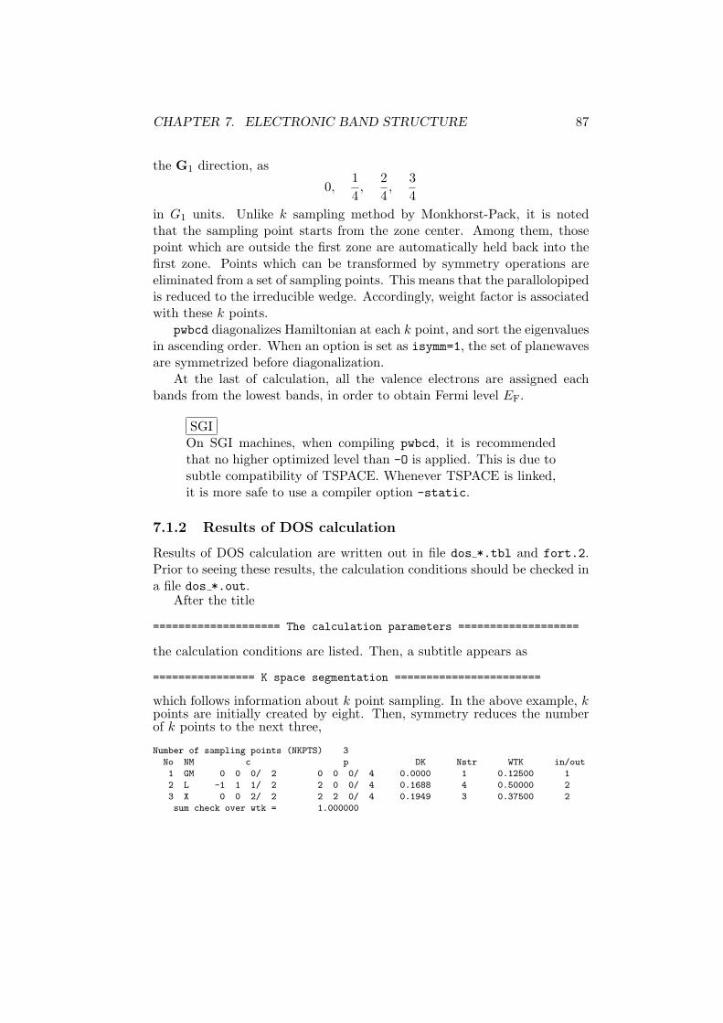
CHAPTER 7. ELECTRONIC BAND STRUCTURE 87
the G1 direction, as
0,1
4,
2
4,
3
4
in G1 units. Unlike k sampling method by Monkhorst-Pack, it is notedthat the sampling point starts from the zone center. Among them, thosepoint which are outside the first zone are automatically held back into thefirst zone. Points which can be transformed by symmetry operations areeliminated from a set of sampling points. This means that the parallolopipedis reduced to the irreducible wedge. Accordingly, weight factor is associatedwith these k points.
pwbcd diagonalizes Hamiltonian at each k point, and sort the eigenvaluesin ascending order. When an option is set as isymm=1, the set of planewavesare symmetrized before diagonalization.
At the last of calculation, all the valence electrons are assigned eachbands from the lowest bands, in order to obtain Fermi level EF.
SGIOn SGI machines, when compiling pwbcd, it is recommendedthat no higher optimized level than -O is applied. This is due tosubtle compatibility of TSPACE. Whenever TSPACE is linked,it is more safe to use a compiler option -static.
7.1.2 Results of DOS calculation
Results of DOS calculation are written out in file dos *.tbl and fort.2.Prior to seeing these results, the calculation conditions should be checked ina file dos *.out.
After the title
==================== The calculation parameters ===================
the calculation conditions are listed. Then, a subtitle appears as
================ K space segmentation =======================
which follows information about k point sampling. In the above example, kpoints are initially created by eight. Then, symmetry reduces the numberof k points to the next three,
Number of sampling points (NKPTS) 3
No NM c p DK Nstr WTK in/out
1 GM 0 0 0/ 2 0 0 0/ 4 0.0000 1 0.12500 1
2 L -1 1 1/ 2 2 0 0/ 4 0.1688 4 0.50000 2
3 X 0 0 2/ 2 2 2 0/ 4 0.1949 3 0.37500 2
sum check over wtk = 1.000000

CHAPTER 7. ELECTRONIC BAND STRUCTURE 88
In this list, the name of k point, the coordinates in the conventional, andin the primitive base appear, which are followed by the magnitude (DK), thenumber of the star, (Nstr), the k point wight (WTK), the index as to whetherinside of the zone or outside (refer TSPACE).
After that, it describes processes of symmetrization of planewaves anddiagonalization of Hamiltonian for each k point. Codes of Osaka2k such aspwm are basically described on the primitive base, while TSPACE is describedon the conventional base. For this reason, pwbcd heavily does conversioncoordinates between these expressions, and checks are made many times.These checks are recorded in file dos *.out. Usual users do not need thisdescription.
dos *.out concludes with estimating Fermi level EF.
=================== determin Ef =================================
Determine the Fermi level
energy --- (eV)
Fermi energy = 6.2896
at 1 th-kpoint 0 0 0/ 4
Total piled up number = 8.000000
Number of electrons = 8
Sorting of HOMO
Valence Top: 6.2896 at 1 2 2 0/ 4
Sorting of LUMO
Conduction Bottom: 7.1785 at 3 0 0 0/ 4
Gap= 0.8889 from 0 0 0/ 4 to 2 2 0/ 4
final distribution of the valence bands
kn IP2 - IP3 E2 - E3 Occ2 - Occ3
1 3 3 - 4 3.17028 - 3.17028 2.00000 - 2.00000
2 2 3 - 4 4.91918 - 4.91918 2.00000 - 2.00000
3 1 2 - 4 6.28963 - 6.28963 2.00000 - 2.00000
Ef= 6.28963 nv= 3 kf= 1 del_n= 0.00000
Nel= 8.0000
Ef= 6.2896
Within the resolution of a given mesh, the energy gap is also estimated. Theabove example says that the energy gap is 0.8889 eV, which is differencebetween the valence top at (000) and the conduction bottom at (220)/4.
After subtitle final distribution of the valence bands, occupa-tions of the valence top bands are displayed over the zone. For Si, becauseit has four valence bands, the forth band is the topmost occupied band,unless there is no degeneracy. When degeneracy takes place, all the degen-erate bands are considered as the valence top level. The band index of these

CHAPTER 7. ELECTRONIC BAND STRUCTURE 89
degenerated top bands are kept by indeces from IP2 to IP3. E2 and E3
are respective energies. In the present case, the degeneracy is rigorous forsymmetry reason. But, even without symmetry reason, those levels whichfall within the energy resolution ERESO are regarded as being degenerate. Inthis case, those bands from IP2 to IP3 are equally occupied. pwbcd checksif the occupation obtained in this way is consistent with the total numberof electron Nel.
7.1.3 Display
For displaying DOS structure, there are two choices.
(i) Line spectrum
The most primitive method to display DOS spectra is simply plot theraw data in dos *.tbl. The format of this file is
1 -5.885658 0.125000
1 6.289627 0.125000
...
2 -3.384971 0.500000
...
The first column lists index of k point, the second does the KS levels, and thethird does the weight of the k point. Mathematica’s notebook DOSshow.nb
reads this file, put these data in Gaussian distribution function, and plotthat. An example obtained in this way is shown in Fig. 7.3 (a).
When using corse mesh points, you see spurious peaks. If you want tolook for van Hove singularity, this is really trouble unless a huge number ofk mesh point is taken.1
(ii) tetrahedron method
The tetrahedron method is a sophisticated algorithm of interpolation forsmoozing discritized DOS curve. [36]
pdosdr do that by reading an output fort.2 of pwbcd, when JobType
= dos. The format of fort.2 will be explained in Sec. 7.2.2. Becausepdosdr is originally created for other use, the way of description for latticeis different from Osaka2k; pwbcd uses the primitive base, while pdosdr uses
1This point is leaned by Prof. Yanase.

CHAPTER 7. ELECTRONIC BAND STRUCTURE 90
nkdiv=4
nkpts=8
nkdiv=8
nkpts=30
=0.1
nkdiv=16
nkpts=149
nkdiv=32
nkpts=913
-10-5 510 15
0.5
=0.05
-10-5 510 15
1
-10-5 510 15
0.5
-10-5 510 15
0.5
1
1.5 =0.2
-10
-10
-5 510 15
1
2
3
-5 510 15
1
2
-5 510 15
1
-5 510 15
1
2
nkdiv=4
nkpts=8
nkdiv=8
nkpts=30
nkdiv=16
nkpts=149
nkdiv=32
nkpts=913
0 10
(a) (b)
Figure 7.3: DOS of Si. (a) line spectra broaden by Gaussian, (b) spectradrawn by the tetrahedron method
the conventional base. For a case such as FCC, user are required to bridgethese two expression in k sampling. 2
For Si case, for example, the Brillouin zone is divided by 2 × 2 × 2 inpwbcd. Because G1, G2, G3 is not orthogonal system, the above meshyields (111)/2 as well as (000) and (001) in the conventional base (2π/aunit ). On the other hand, pdosdr divides uniformly the space a∗, b∗, c∗,because of use of conventional base. If we set the division number two, extrapoints such as (100)/2, (110)/2, in addition to the above k points. As tothese extra points, because pwbcd does not sample, this setting causes errorin pdosdr.
Hence, in pdosdr, the division number should be 1. Then, pdosdr takes
2The authors did not check completely for all crystal systems, although he believescorrectness of the present treatment.

CHAPTER 7. ELECTRONIC BAND STRUCTURE 91
four k points, i.e., (000)/1, (100)/1, (110)/1, (111)/1. Because (111)/1 isequivalent to (000)/1, and (110)/1 is to (100)/1, among three k points inpwbcd, only two are used in pdosdr. The other is discarded. This waste ofcomputation cannot be helped.
Now, we explain how to use pdosdr. Prepare an input file pdos.para,as
NONMSPIN-ORBIT
1 1 1
0
-10.0 20.0 0.2
8
The first line is related to magnetic states, and in the present case,simply follow the above example. The next three numbers indicate thedivision numbers in the k space, NX, NY, and NZ. Care must be paid in orderto keep consistency the division numbers in pwbcd, as described above. Thenext line is set to be zero, which is used for decomposition of DOS intoatomic orbitals. The following three numbers are the lower limit of energyaxis (ESTART), the upper limit (ENEND, the width of energy step (DE). Themesh points of the energy axis are therefore ENEND-ESTART)/DE+1 The lastnumber is the number of electrons in the primitive unit cell
An output file fort.12 lists as
SPIN 1
1 -10.0000 0.000 0.0000
2 -9.8000 0.000 0.0000
150 19.8000 1.689 27.1343
151 20.0000 1.438 27.4481
electron number= 8 EF= 6.80000000000000
The spectrum data are listed between the first and last comment lines. Eachline lists the index of energy mesh, energy, DOS, and its convolution up tothis point.
This data can be displayed by Mathematica’s notebook PDOSshow.nb.By removing the first and last lines of fort.12, it is read by PDOSshow.nb.In Fig. 7.3 (b), an example is shown. Even when mesh points are small,DOS curve looks smooth. But, if you want to obtain van Hove singularities,it is invariably true that you have to take a large number of mesh points.
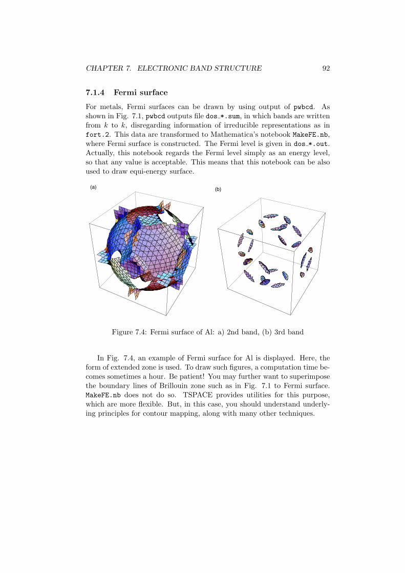
CHAPTER 7. ELECTRONIC BAND STRUCTURE 92
7.1.4 Fermi surface
For metals, Fermi surfaces can be drawn by using output of pwbcd. Asshown in Fig. 7.1, pwbcd outputs file dos *.sum, in which bands are writtenfrom k to k, disregarding information of irreducible representations as infort.2. This data are transformed to Mathematica’s notebook MakeFE.nb,where Fermi surface is constructed. The Fermi level is given in dos *.out.Actually, this notebook regards the Fermi level simply as an energy level,so that any value is acceptable. This means that this notebook can be alsoused to draw equi-energy surface.
(b)(a)
Figure 7.4: Fermi surface of Al: a) 2nd band, (b) 3rd band
In Fig. 7.4, an example of Fermi surface for Al is displayed. Here, theform of extended zone is used. To draw such figures, a computation time be-comes sometimes a hour. Be patient! You may further want to superimposethe boundary lines of Brillouin zone such as in Fig. 7.1 to Fermi surface.MakeFE.nb does not do so. TSPACE provides utilities for this purpose,which are more flexible. But, in this case, you should understand underly-ing principles for contour mapping, along with many other techniques.

CHAPTER 7. ELECTRONIC BAND STRUCTURE 93
7.2 Band structure
The band calculation in pwbcd calculates bands at k points along arbitrarylines, although the lines are usually chosen to be symmetry lines. Theselines should be singly connected. As in DOS case, two ways for displaythe result are ready. One is simply plot each bands without information ofsymmetry, by reading file band *.tbl. The other is sophisticated method ofusing ayband, which interpolates and extrapolates points by using symmetryproperties fully. Outputs of ayband is PostScript file. Then, the file can behandled by many drawing programs, such as Illustrator. ayband is createdby Prof. A. Yanase.
7.2.1 Preparation
For band calculation, input file bcd.para looks like
JobType
bnd
Input file name
si.prim
number of k points specifying symmetry lines (NKPTS)
7
KB(3), ICB (in prim)
0 0 0 1 G
3 3 6 8 K
1 1 2 2 X
1 2 3 4 W
1 1 1 2 L
0 0 0 1 G
0 1 1 2 X
number of division per line (NDIV)
5
number of levels you want to draw (NBUP) usually NEPC
12
scan zone only (iscan)
1
print control (ilp)
1
use symmetry (isymm)
1
In the following, meaning of each parameter is described.The most important input is specification of lines, on which band disper-
sions are drawn. pwbcd assumes that the drawing lines are singly connected.Hence, the drawing lines are expressed by sequence of node points k as
A → B → C · · ·
The number of nodes is given by NKPTS in bcd.para. Then, each node pointk, KB(3)/ICB, is given in primitive base.
CHAPTER 7. ELECTRONIC BAND STRUCTURE 94
JobType Job type = bndxtl.name crystal nameNKPTS number of lines drawnKB(3), ICB terminal k points of each lineNDIV division number for each lineNBUP number of bands drawniscan options for debug 1: defaultilp print option 1: defaultisymm option for symmetrization 1: on, 0: off
In the above example, five symmetry lines, L−Γ, Γ−X, X−W , W −K,K − Γ, are taken. 3 The segment number of each line is given by NDIV.
The number of bands which you want to draw is specified by NBUP. pwbcdcalculates bands from the lowest up to NBUP at each k point. As in DOS, itmay be as large as the number of electrons in the primitive unit cell. But, iftoo small, it should be more than that. When setting use symmetry = 1,this caution is particularly important. In this case, pwbcd enumerates bandsat each symmetry block by NBUP. If NBUP is too small, it may happen for someband on a symmetry line to miss to connect to that on another symmetryline. In this case, NBUP should be increased. The remaining parameters arefor debug purpose, so usually there are left as it.
7.2.2 Result of band calculation
pwbcd calcultes bands along given lines, and yields output file bnd *.tbl andfort.2. Before seeing result, users should check if the calculation conditionsare really what you intend. This can be seen in file bnd *.out, as in DOS.
For quick view band diagram, data bnd *.tbl is transformed to a 2-dimensional plotting program. The format of bnd *.tbl looks like
1 -0.248790244660327
1 -6.646822029304370E-002
...
2 -0.289100855937076
...
In each line, first the index of k point comes, then an energy level comes.Therefore, plotting it is easy. An example obtained in this way is shown in
3Prof. A. Yanase points out a wise selection Γ → K → X(1, 1, 0) → W → L → Γ →
X(1, 0, 0)

CHAPTER 7. ELECTRONIC BAND STRUCTURE 95
Fig. 7.5. The abscissa represents k lines in order L − Γ − X − W − K − Γ,and each line is segmented by 5. Due to lack of symmetry information,connectivity between adjacent levels has to been decided manually. In thisexample, this determination is not difficult, but for more general case, am-biguity always is associated with. At the zone boundary, sometimes theasymptotic behavior of dispersion of degenerate bands is important. In thiscase, symmetry properties help us greatly to remove such ambiguities. But,full use of symmetry properties are highly skillful work, so that user shouldlean deeply group-theoretical methods.
3020100-0.5
0.0
0.5
1.0
1.5
k
EE
Figure 7.5: Primitive plotting of bands of Si. The output of pwbcd is simplyplotted without use fo symmetry properties.
ayband does this in place of you. ayband connects relevant pointssmoothly by spline curves. To which point should be connected to which isjudged by using irreducible representations. Also, for curvature at the zoneboundary, ayband checks if k dependence is linear in k or quadric, by usingcumbersome processes which are seemingly redundant calculations.

CHAPTER 7. ELECTRONIC BAND STRUCTURE 96
Two bands which belong to the same irreducible presentation do not cross, i.e., no
closing rule. Accordingly, there is no accidental degeneracy. ayband is strict with
this principle. I have no compliant with this treatment in implementation, because
actual code should have always definite criteria, otherwise we could not write code.
However, I am not sure if this is in principle correct. For example, C. Herring
discussed various properties of accidental degeneracy if the accidental degeneracy
presents.[37] I am not sure if accidental degeneracy without any symmetry reason
can happen.
Output file fort.2 is a complete data set in terms of symmetry proper-ties. This file is expected to put in ayband.
The data format of fort.2 is as follows.Data are gathered according to k points, while in each k point data are
gathered according to the irreducible representation of the small group of k.The minimum data block looks like
1 5 5 5 10 1 L 2 1 1 5
2.793676 5.247479 6.851224 7.409376 8.271489
The first number is a serial number, which follows the next four representk in presentation KB(3)/IC. In this examle, (5, 5, 5)/10, that is, L point.User should note that k is presented in the conventional base. Next comesa spin-related parameter (IUD), which follows the name of k point.
The remaining four are the index of the irreducible representation (MRN),the dimensionality of the representation (MWET), the number of star k (NST),and the number of eigenstates belonging this block (NEIG).
After carried return, NEIG eigenvalues are enumerated in ascending orderin energy.
ayband uses information involved in fort2.In order to execute ayband, further input data are required. fort.3 is
another input file. There contains parameters to control drawing process.The format looks like
NONMSPIN-ORBIT
0 0 50 NLCOMP NSPIN IFILE
0 1 12 JPR JMARK IPOINT(character)
-1.0 1.2 100.0 150.0
5
4 4 4 8 0 0 0 8 LD
0 0 0 8 8 0 0 8 DT
8 0 0 8 8 4 0 8 W
8 4 0 8 6 6 0 8 K

CHAPTER 7. ELECTRONIC BAND STRUCTURE 97
6 6 0 8 0 0 0 8 SM
0.5 Fermi level
Si PseudoPotential
The meaning of these parameters are described in the following.
MAGNET Magnetic state. pwm uses option NONMSPIN-ORBIT only.
NLCOMP, NSPIN,IFILE the number of DOS components with respectto angular-momentum, spin state. Set both to be 0. IFILE is the fileindex of the output file.
IPR, JMARK,IPOINT The first two are parameters controlling output.By default, set as in the above. IPOINT is the size of characters forthe representation in the band diagram. item [E0, EM, YM, XM]Minimum and maximum of energy of plotting, and the scale of x−and y− axis in mm.
NAXM the number of lines in band diagram. Individual lines are describedin the following.
line description Specify symmetry lines by giving two terminal points k1
and k2. k is given three numerators and the common denominator.This description appears for NAXM lines. The name of terminal pointsare added for users convenience only, and are not read in ayband.
EF Fermi level
TITLE The title of figure
In this way ayband requires again line specifications, independent of thoseof pwbcd.
In Fig. 7.6, a band diagram obtained in this way is displayed.You can see that dispersion curves are smoothly drawn, and connectivity
at the zone boundary is made clear.
In the figure, the numbers indicate the label of irreducible representa-tion. This numbering is in accordance with TSPACE, the way of which is itsown one. Users who have well read reference may want to use more ortho-dox labeling. In this case, user are expected to examine correspondence oflabeling between TSPACE and the reference you want.
CHAPTER 7. ELECTRONIC BAND STRUCTURE 98
-0.6-0.5-0.4-0.3-0.2-0.1 0.0 0.1 0.2 0.3 0.4 0.5 0.6 0.7 0.8 0.9 1.0 1.1 1.2 1.3 1.4
Ener
gy \
Ry\
Γ Σ KS X Z W Q L Λ Γ ∆ X
1
1
1
1
4 46 6
7
7
7
7
A A
1
1
1
1
1
2
2
3
4
4
4
4
4
1
1
1
1
2
2
3
4
4
4
4
4
1
1
1
1
2
2
3
4
4
4
4
1
1
11
2
2
3
4
4
4
1
1
1
1
2
2
3
4
4
4
1
1
1
1
2
2
3
4
4
4
1
1
1
1
2
2
3
4
4
4
1
1
1
1
2
2
3
4
4
4
1
1
1
1
2
2
3
4
4
4
1
1
1
1
1
1
1
1
1
1
1
1
1
1
1
1
1
1
1
1
1
1
1
2
2
1
1
1
1
1
2
2
2
2
2
1
1
1
1
1
2
2
2
22
2
1
1
1
1
1
1
2
2
2
2
2
2
1
1
1
1
1
1
2
2
2
2
2
2
1
1
1
4
4
4
5
5
6
6
1
1
1
1
1
3
3
3
1
1
1
1
1
1
3
3
3
1
1
1
1
1
1
3
3
3
1
1
1
1
1
1
3
3
3
3
1
1
1
2
4
4
4
4
5
5
5
1
1
12
4
4
4
5
5
1
1
12
4
4
4
5
5
1
1
2
4
4
4
5
5
2
2
2
2
2
2
3 3
4 4
EF
Si PseudoPotential
Figure 7.6: band diagram of Si drawn by ayband. The line lengths of dif-ferent k points are given by the correct length in k space
As to time-reversal symmetry, a note should be added. When time-
reversal symmetry yields extra degeneracy between different irreducible
representations, ayband displays only one of them. For example, a
zincblend crystal (S.G. T 2d ) such as GaAs has extra degeneracy be-
tween ∆3 and ∆4 on ∆ line, due to time-reversal symmetry. ayband
attributes only 3 as the label. Therefore, when you enumerate bands
and degeneracy, you should count by taking another invisible one into
account.
A troublesome point of character table in the literature is that there areactually two ways of presentations; normal irreducible representation (vectorpresentation) and ray presentation (projective or multiplier representation).4 TSPACE uses ray presentation. In my impression, vector representation ismore frequently used in the literature of band calculations. Maybe, Koster
4An example of the vector representation is Koster[38]. This representation is easy tounderstand, but actual character table is apt to be big. Enumeration of this representation

CHAPTER 7. ELECTRONIC BAND STRUCTURE 99
table [38] is one of the most frequently cited one. Therefore, the corre-spondence of representations between TSPACE and literature such as Koster,BSW, etc.
TSPACE can print out complete list of irreducible tables by calling TSIRDS.TSPACE uses ray representation D(α). It is an irreducible representation Γ(α)of the small group k multiplied by a phase factor
D(α) = exp(ik · τα)Γ(α), (7.1)
where τα is a nonprimitive translation associated with rotation α This rep-resentation D(α) looks neat because superfitious factor associated with non-primitive translation is removed, and thereby has definite correspondence tothe point group except zone boundary.
Let us see an example of nonsymmorphic space group, say, Si. On ∆line, subroutine TSIRDS prints out character tables, as
IMR NO 1 DIMENSION= 1
1 2192227284042
1 1 + + + + + + + +
IMR NO 2 DIMENSION= 1
1 2192227284042
1 1 + + + + - - - -
IMR NO 3 DIMENSION= 1
1 2192227284042
1 1 + + - - + + - -
IMR NO 4 DIMENSION= 1
1 2192227284042
1 1 + + - - - - + +
IMR NO 5 DIMENSION= 2
1 2192227284042
1 1 + - I J 0 0 0 0
2 2 + - J I 0 0 0 0
in file fort.15. In this table, all the matrix element for all the symmetryelements are listed (In the present, only diagonal elements are extracted forclarity). Meaning of the index of symmetry elements and index of repre-sentation should be referred to in TSPACE [24]. The character of this raypresentation is compiled to show in the left of Table 7.1.
By seeing this, you can find definite correspondence of character tablebetween the present D(α) and that of point group C4v. On the other hand,in the vector representation Γ(α), complex number η appear. In the limit
for all 230 space groups is tremendous task. On the contrary, ray representation achievesgreatly economy of table. Hence, Kovalev[39], Bradley Cracknell [40] thoroughly describescharacter tables which cover all the space group. Ray representation is, on the other hand,higher skill to understand.
CHAPTER 7. ELECTRONIC BAND STRUCTURE 100
Table 7.1: Character table on the ∆ line. The left shows multiplier represen-tations D, while the right shows vector representations Γ. The second rowlists non-primitive translation τ = (1/4, 1/4, 1/4) associated with rotation.The first column of the left part indicates the label in TSPACE.
D E C2 2C4 2σv 2σd Γ E C2 2C4 2σv 2σd
τ τ τ τ1 ∆1 1 1 1 1 1 ∆1 1 1 η η 12 ∆′
1 1 1 1 -1 -1 ∆′1 1 1 η −η -1
3 ∆2 1 1 -1 1 -1 ∆2 1 1 −η η -14 ∆′
2 1 1 -1 -1 1 ∆′2 1 1 −η −η 1
5 ∆5 2 -2 0 0 0 ∆5 2 -2 0 0 0η = exp[−ik · τ ]
k → 0, this factor becomes 1, so that you can still find correspondence tothe presentation of the point group C4v.
But, at the zone boundary, it is not easy. When the dimension of arepresentation is one, the representation becomes equivalent to that of pointgroup, but complex numbers appear in the character. When the dimension ismore than one, correspondence to that of point group disappears. Probably,irreducible representations of X point is the most complicated one. The raypresentation looks like,
IMR NO 1 DIMENSION= 2
1 2 3 4161819222526272840424346
1 1 + + + + 0 0 0 0 0 0 0 0 - - - -
2 2 + + - - 0 0 0 0 0 0 0 0 - - + +
IMR NO 2 DIMENSION= 2
1 2 3 4161819222526272840424346
1 1 + + + + 0 0 0 0 0 0 0 0 + + + +
2 2 + + - - 0 0 0 0 0 0 0 0 + + - -
IMR NO 3 DIMENSION= 2
1 2 3 4161819222526272840424346
1 1 + - + - J I J I 0 0 0 0 0 0 0 0
2 2 + - - + J I I J 0 0 0 0 0 0 0 0
IMR NO 4 DIMENSION= 2
1 2 3 4161819222526272840424346
1 1 + - + - I J I J 0 0 0 0 0 0 0 0
2 2 + - - + I J J I 0 0 0 0 0 0 0 0
As before, it is arranged as the character table in the left of Table 7.2.As Koster table [38] lists only vector representations (the right of Table
7.2), the characters converted to the vector representation Γ(α) by Eq. (7.1)are written in output file fort.18 of pwbcd. There, character tables arelisted at each k point.
11 1 th point = 40 0 0/ 40 X 2 1.0000 0.0000 0.0000
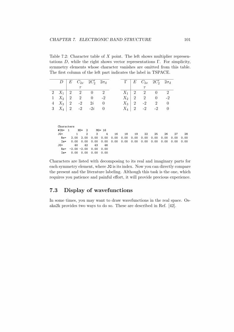
CHAPTER 7. ELECTRONIC BAND STRUCTURE 101
Table 7.2: Character table of X point. The left shows multiplier represen-tations D, while the right shows vector representations Γ. For simplicity,symmetry elements whose character vanishes are omitted from this table.The first column of the left part indicates the label in TSPACE.
D E C2x 2C ′2 2σd Γ E C2x 2C ′
2 2σd
τ τ2 X1 2 2 0 2 X1 2 2 0 21 X2 2 2 0 -2 X2 2 2 0 -24 X3 2 -2 2i 0 X3 2 -2 2 03 X4 2 -2 -2i 0 X4 2 -2 -2 0
Characters
#IR= 1 ND= 2 MG= 16
JG= 1 2 3 4 16 18 19 22 25 26 27 28
Re= 2.00 2.00 0.00 0.00 0.00 0.00 0.00 0.00 0.00 0.00 0.00 0.00
Im= 0.00 0.00 0.00 0.00 0.00 0.00 0.00 0.00 0.00 0.00 0.00 0.00
JG= 40 42 43 46
Re= -2.00 -2.00 0.00 0.00
Im= 0.00 0.00 0.00 0.00
Characters are listed with decomposing to its real and imaginary parts foreach symmetry element, where JG is its index. Now you can directly comparethe present and the literature labeling. Although this task is the one, whichrequires you patience and painful effort, it will provide precious experience.
7.3 Display of wavefunctions
In some times, you may want to draw wavefunctions in the real space. Os-aka2k provides two ways to do so. These are described in Ref. [42].

Appendix A
Graphics display of a crystalby Mathematica
A.1 coordinates systems
Most of graphics data of Osaka2k can be handled by Mathematica’s note-books. Among these nobebooks, only ChgDnst.nb is described in this ap-pendix. Because projecting of charge density distribution on a cross sectionis frequently used, user should be familiar to handle the coordinate systemin a general way. Nowadays, there are many commercial programs are avail-able to display such a distribution. Nevertheless, you cannot use it withfoolproof. I mean that without knowledge of coordinate system and of howsurfaces are expressed, you cannot obtain correct answer. Efforts for un-derstanding how express nonorthogonal system and how specify a cut planein a particular program, even it is a well documented commercial program,amounts to almost the same effort to create the same program. You mustknow what you are doing with a specific coordinate.
Here, as nontrivial example, we take α oxigen crystal, which belongs tomonoclinic crystal. The space group is C2/m, and base-center (C-center),and the crystal structure is shown in A.1 (a).
Basically, Mathematica’s 3-dimensional plotting routines assume to useequi-spacing orthogonal mesh. Owing this, tedious conversion of coordinatesare required for non-orthogonal systems. Although user are not required toknow details of coordinate transformation, he must know how specify a cutplane he wants to draw.
In ChgDnst.nb, by section 2. (Construct crystal structure), a given
102

APPENDIX A. GRAPHICS DISPLAY OF A CRYSTAL BY MATHEMATICA103
(a)
(b)
R1R2
R3
ab
c
gp0
gp1gp2
gp4
gp3
gp7gp5
gp6pl0
pl2
pl1
(c)
pl0 pl1
pl2plt
Figure A.1: Cutting a cross section out of the crystal. (a) α− oxigen crysal.The primitive unit cell (red) and the conventional unit cell (blue) are indi-cated. Graphics frame covers both of unit cells. (b) a cut plane (green) isspecified by three points, pl0, pl1, pl2. (c) 2-dimensional charge densityis plotted on the rectangular spanned by pl0, pl1, plt
crystal is described in the folloing, First, in section read *.prim, data ofthe crystal structure is read by opening data file
file = OpenRead["name.prim"]
Hence, you should input the name of a crystal file.The length unit is given by the maximum of a0, b0, c0 (amax in A)
• The primitive unit cell is given by three primitive translational vectorst1, t2, t3 ( t1, t2, t3 in the notebook)
• The conventional unit cell is given by three translational vectors tc1, tc2, tc3( tc1, tc2, tc3)

APPENDIX A. GRAPHICS DISPLAY OF A CRYSTAL BY MATHEMATICA104
• Define a global region so that it includes all these unit cells. Theglobal region is spanned by three vectors gp1, gp2, gp3 ( gp1, gp2,
gp3), and these are necessarily an orthogonal set.
Given these basic data, ChgDnst.nb draws the primitive and conven-tional unit cells, and cut the global region, as shown in Fig. A.1 (a). Theglobal region is a parallelepiped, whose vertices are termed as gp0, . . . , gp7(in the figure (b)). In what follows, all coordinates are expressed on thisglobal coordinates.
In this coordinate system, atom positions are expressed as follows.
• The basis are composed of Natom (natom) atoms. The positions aregiven by ba[i].
• Lattices are specified by a set of three integers. This is done in thenotebook by calling function lattice
lattice[l_,m_,n_] := N[l t1+m t2+n t3]
In convenience, several of these are identified by a serial number, as
lattice[0]=lattice[0,0,0];
lattice[1]=lattice[1,0,0];
lattice[2]=lattice[0,1,0];
lattice[3]=lattice[0,0,1];
lattice[4]=lattice[1,1,0];
lattice[5]=lattice[0,1,1];
lattice[6]=lattice[1,0,1];
lattice[7]=lattice[1,1,1];
lattice[8]=lattice[-1,1,1];
lattice[9]=lattice[1,-1,1];
lattice[10]=lattice[1,1,-1];
lattice[11]=lattice[1,-1,0];
lattice[12]=lattice[1,0,-1];
lattice[13]=lattice[0,1,-1];
lattice[14]=lattice[2,0,0];
lattice[15]=lattice[0,2,0];
lattice[16]=lattice[0,0,2];
and
lattice[-#]=-lattice[#];
• Atom positions are given by calling function atomPos
atomPos[l_Integer,j_Integer]:=lattice[l]+ba[j]

APPENDIX A. GRAPHICS DISPLAY OF A CRYSTAL BY MATHEMATICA105
This is a list of major variables in the notebook.Another complication can occur for the present case of oxigen crystal.
When the graphics region is clipped by the global region, gp0, . . . , gp7,a molecule O2 is halfway cut. Accordingly, the molecular unit is hardlyseen. Therefore, user should expand the global region further. This is donemanually, by following the algorithm of the notebook.
After that, in section read data file, input the file name of chargedensity, as
file = OpenRead["pwm_name.rho"]
Then, charge density data are read in. After the title, density statistics
ro3min, atmin
0.234258, 1, 1, 35
ro3max, atmax
247.381, 12, 58, 56
ChgDnst.nb calculates the maximum and minimum of charge density.3-dimensional contour map of charge density is plotted by scanning data
points inside the global parallelepiped region. User achieves it only by throw-ing desired parameters in plot command
Timing[ grf = ContourPlot3D[ fulst[l,m,n],
l,igxmin,igxmax,m,igymin,igymax,n,igzmin,igzmax,
Contours->80, PlotPoints->8,4 ] ]
Here, Contours is the value of contour at which contour map is created.Hence, this value must be fallen into a range between the mimimum andmaximam of charge density, estimated before. Fig. 5.4 is an example ob-tained in this way in a global region, gp0, ... , gp7.
A 2-dimensional cut plane is specified by two vectors. These are spec-ified by three points, pl0, pl1, pl2. It is recommended that these threepoints are expressed by using gp0, ... , gp7 instead of using absolutecoordinates. If you want to take pl0 a quarter of gp0-gp3, define it as
−→pl0 =
3−→gp0 +
−→gp3
4(A.1)
The right-hand side contains gp0, ... , gp7 only.Because the region spanned by the vectors is, in general, not rectangular,
a new vector plt is taken as normal to a line pl0-pl1 as shown in the figure

APPENDIX A. GRAPHICS DISPLAY OF A CRYSTAL BY MATHEMATICA106
A P
Figure A.2: Coordinate transformation in displaying charge density plot.The primitive unit cell is indicated by red lines, while black frames indicatethe global region. Charge density is given at each lattice point. Point Agiven in the cartesian coordinates is draw back to an equivalent point P inthe primitive unit cell.
(c). The black area if the final region on which contour map is drawn. InChgDnst.nb, intersections of the unit cell and atom positions, if any, aredrawn as well. An example is shown in Fig. 5.5.
A.2 Charge density contour map
The charge density data in the real space, rod r, are given on the primitiveunit cell only, because it is a minimum set. The primitive unit cell is dividedby na1, na2, na3 , and the charge density is given only those lattice
points. The normalized factor is taken to satisfy
Nel =NA3∑
i=1
ρi ×1
NA3, (A.2)
where Nel is the number of electrons in the primitive unit cell
After charge density data are read in the notebook, the charge densityis transacted. There are two points to be considered.

APPENDIX A. GRAPHICS DISPLAY OF A CRYSTAL BY MATHEMATICA107
First, it is almost always better to expand charge density data on thecartesian lattice points in order to proceed with graphics processes. Onthe other hand, the original primitive cell on which the lattice points areexpanded is in general not an orthogonal system. Even cubic crystals, FCCand BCC are not orthogonal systems.
Another point is that, because the original data are given only inside theprimitive unit cell, in order to obtain the charge density at a general pointin the whole space, the general point is hold back into the primitive unitcell.
By these requirements, conversion of the coordinates between the carte-sian and the original primitive unit cell space is needed. These relation isshown in Fig. A.2.
This conversion is carried out by function
fd[l_,m_,n_]
in notebook. This function is calculate the charge density at a general pointon the whole space. A point A on which you want to know the charge densityis given by the cartesian coordinate l, m, n. This point is draw back topoint P in the primitive unit cell as shown in Fig. A.2. The primitiveunit cell is originally divided by na1, na2, na3 . Because the point P
is generally not a lattice point in the primitive unit cell, the charge densityof P is interpolated by those of the nearest neighbor lattice points. Theinterpolated value is return by function fd.
All the contour maps of charge density are drawn through calling fd.

Acknowledgment
In the course of developing Osaka2k, contribution of pioners has been de-scribed in Introduction. Here, I like express my gratitude to other people,mainly students of our laboratory. Particular, H. Fujita and Y. Yamazakicontributed at the initial stage of the project, which is usually the mostdifficult time. Dr. Dinh van An helped me to translate the part of theoryin this manual.
108
References
[1] P. Hohenberg and W. Kohn, Phys. Rev. 136, B864 (1964)
[2] W. Kohn and L. J. Sham, Phys. Rev. 140, A1133 (1965)
[3] J. Callaway and N. H. March, Solid Stete Physics 38, (1984) p. 135
[4] R. O. Jones and O. Gunnarsson, Rev. Mod. Phys. 61, 689 (1989)
[5] Adv. in Quantum Chemistry 21, S. B. Trickey ed., (Academic, SanDiego, 1989)
[6] D. M. Ceperley and B. Alder, Phys. Rev. Lett. 45, 566 (1980)
[7] J. P. Perdew and A. Zunger, Phys. Rev. B 23, 5048 (1981)
[8] V. Heine, Solid Stete Physics 24, (1970) p. 1, and all the volume.
[9] D. R. Hamann, M. Schluter, and C. Chiang, Phys. Rev. Lett. 43, 1494(1979)
[10] N. Troullier and J. L. Martins, Phys. Rev. B 43, 1993 (1991)
[11] L. Kleinman and D. M. Bylander, Phys. Rev. Lett. 48, 1425 (1982)
[12] G. B. Bachelet, D. R. Hamann, and M Schluter, Phys. Rev. B 26, 4199(1982)
[13] N. W. Aschcroft and N. D. Mermin, ”Solid State Physics”, (Holt-Saunders, Philadelphia, 1976)
[14] J. Ihm, A. Zunger, and M. L. Cohen, J. Phys. C: Solid State Phys. 12,4409 (1979)
[15] M. Born and K. Huang, ”Dynamical Theory of Crystal Lattices”, (Ox-ford University Press, Oxford, 1954)
109

REFERENCES 110
[16] H. J. Monkhorst and J. D. Pack, Phys. Rev. B 13, 5188 (1976)
[17] W. H. Press, S. A. Teukolsky, W. T. Vetterling, and B. R. Flannery,”Numeric Recipes”, 2nd ed. (Cambridge, Camridge, 1992)
[18] M .P .Teter, M. C. .Payne, and D. C. Allan, Phys. Rev. B 40, 12255(1989)
[19] M. C. .Payne, M .P .Teter, D. C. Allan, T .A .Arias, andJ .D Joannopoulos, Rev. Mod. Phys. 64, 1045 (1992)
[20] R. Car and M. Parrinello, Phys. Rev. Lett. 55, 2471 (1985)
[21] R. P. Feynman, Phys. Rev. 56, 340 (1939)
[22] O. H. Nielsen and R. M. Martin, Phys. Rev. B 32, 3780 (1985)
[23] O. H. Nielsen and R. M. Martin, Phys. Rev. B 32, 3792 (1985)
[24] A. Yanase, Fortran Program for Space Group (TSPACE), (Shokabo,Tokyo, 1995)
[25] T. Hahn, ed. ”International Tables for Crystallography”, Vol. A(Kluwer Academic Pub., Dordrecht, 1996)
[26] G. Burns and A. M. Glazer, ”Space Groups for Solid State Scientists”,2nd. ed., (Academic, San Diego, 1990)
[27] M. T. Yin and M. L. Cohen, Phys. Rev. B 26, 3259 (1982)
[28] J. Ihm and M. L. Cohen, Phys. Rev. B 21, 1527 (1980)
[29] J. Stoer and R. Bulirsch, ”Introduction to Numerical Analysis”, 2nded. (Springer, New York, 1992)
[30] D. J. Chadi and M. L. Cohen, Phys. Rev. B 8, 5747 (1973)
[31] C. H. Park, B.-H. Cheong, K. H. Lee, and K. J. Chang, Phys. Rev. B49, 4485 (1994)
[32] J. Callaway, ”Quantum Theory of the Solid State”, 2nd. ed., (Academic,San Diego, 1991).
[33] C. -L. Fu and K. -M. Ho, Phys. Rev. B 28, 5480 (1983)
[34] M. R. Pederson and K. A. Jackson, Phys. Rev. B 43, 7312 (1991)

REFERENCES 111
[35] M. T. Yin, Proc. 17th Int. Conf. on the Physics of Semiconductors, eds.J. D. Chadi and W. A. Harrison (Springer, NY, 1984) p. 927
[36] O. Jepson and O. K. Anderson, Solid State Commun. 9, 1763 (1971)
[37] C. Herring, Phys. Rev. 52, 365 (1937)
[38] G. F. Koster, Solid Stete Physics 5, (1957) p. 173. It is sometimespointed out that there are errors in the printed character tables inthe literature, including this Koster’s paper. Errors found in the majorprinted tables are corrected in J. L. Warren, Rev. Mod. Phys. 40, 38(1968).
[39] O. V. Kovalev, ”Representations of the Crystallographic SpaceGroups”, 2nd ed., translated to English (Gordon adn Breach ScientificPub., Yverdon, 1993)
[40] C. J. Bradley and A. P. Cracknell, ”The Mathematical Theory of Sym-metry in Solids”, (Clarendon Press, Oxford, 1972)
[41] L. Verlet, Phys. Rev. 159, 98 (1967)
[42] Technical Report No. 21 ”Plotting of wavefunctions on the real space”
[43] D. Frenkel and B. Smit, ”Understanding Molecular Simulation”, (Aca-demic, San Diego, 1996)
[44] S. E, Koonin and D. C. Meredith, ”Computational Physics”, (AddisonWesley, Massachusets, 1990)