Submitted 2017 October 17; revised 2018 May 8; accepted 2018 June 4Preprint typeset using LATEX style emulateapj v. 12/16/11

FIRST ALMA LIGHT CURVE CONSTRAINS REFRESHED REVERSE SHOCKS & JET MAGNETIZATION INGRB161219B

Tanmoy Laskar1,2,3, Kate D. Alexander4, Edo Berger4, Cristiano Guidorzi5, Raffaella Margutti6,Wen-fai Fong6,7, Charles D. Kilpatrick8, Peter Milne9, Maria R. Drout10,11, C. G. Mundell12,

Shiho Kobayashi13, Ragnhild Lunnan14,15, Rodolfo Barniol Duran16, Karl M. Menten17, Kunihito Ioka18,Peter K. G. Williams4

Submitted 2017 October 17; revised 2018 May 8; accepted 2018 June 4

ABSTRACT

We present detailed multi-wavelength observations of GRB161219B at z = 0.1475, spanning theradio to X-ray regimes, and the first ALMA light curve of a GRB afterglow. The cm- and mm-band observations before 8.5d require emission in excess of that produced by the afterglow forwardshock (FS). These data are consistent with radiation from a refreshed reverse shock (RS) producedby the injection of energy into the FS, signatures of which are also present in the X-ray and opticallight curves. We infer a constant-density circumburst environment with an extremely low density,n0 ≈ 3 × 10−4 cm−3, and show that this is a characteristic of all strong RS detections to date. TheVLA observations exhibit unexpected rapid variability on ∼ minute timescales, indicative of stronginterstellar scintillation. The X-ray, ALMA, and VLA observations together constrain the jet breaktime, tjet ≈ 32d, yielding a wide jet opening angle of θjet ≈ 13, implying beaming corrected γ-rayand kinetic energies of Eγ ≈ 4.9× 1048 erg and EK ≈ 1.3× 1050 erg, respectively. Comparing the RSand FS emission, we show that the ejecta are only weakly magnetized, with relative magnetization,RB ≈ 1, compared to the FS. These direct, multi-frequency measurements of a refreshed RS spanningthe optical to radio bands highlight the impact of radio and millimeter data in probing the productionand nature of GRB jets.

Keywords: gamma-ray burst: general – gamma-ray burst: individual (GRB161219B)

1. INTRODUCTION

1 National Radio Astronomy Observatory, 520 EdgemontRoad, Charlottesville, VA 22903, USA

2 Department of Astronomy, University of California, 501Campbell Hall, Berkeley, CA 94720-3411, USA

3 Jansky Fellow4 Department of Astronomy, Harvard University, 60 Garden

Street, Cambridge, MA 02138, USA5 Department of Physics and Earth Science, University of Fer-

rara, via Saragat 1, I-44122, Ferrara, Italy6 Center for Interdisciplinary Exploration and Research in

Astrophysics (CIERA) and Department of Physics and Astro-physics, Northwestern University, Evanston, IL 60208, USA

7 Hubble Fellow8 Department of Astronomy and Astrophysics, University of

California, Santa Cruz, CA 95064, USA9 Steward Observatory, University of Arizona, 933 N. Cherry

Ave, Tucson, AZ 85721, USA10 Hubble and Carnegie-Dunlap Fellow11 The Observatories of the Carnegie Institution for Science,

813 Santa Barbara Street, Pasadena, CA 91101, USA12 Department of Physics, University of Bath, Claverton

Down, Bath, BA2 7AY, United Kingdom13 Astrophysics Research Institute, Liverpool John Moores

University, IC2, Liverpool Science Park, 146 Brownlow Hill, Liv-erpool L3 5RF, United Kingdom

14 The Oskar Klein Centre & Department of Astronomy,Stockholm University, AlbaNova, SE-106 91 Stockholm, Sweden

15 Department of Astronomy, California Institute of Technol-ogy, 1200 East California Boulevard, Pasadena, CA 91125, USA

16 Department of Physics and Astronomy, California StateUniversity, Sacramento, 6000 J Street, Sacramento, CA 95819,USA

17 Max-Planck-Institut fur Radioastronomie, Auf dem Huegel69, 53121 Bonn, Germany

18 Center for Gravitational Physics, Yukawa Institute for The-oretical Physics, Kyoto University, Kyoto 606-8502, Japan

Long-duration γ-ray bursts (GRBs) have thus farbeen almost exclusively discovered through theirprompt γ-ray emission, which unequivocally arisesfrom relativistic outflows at high Lorentz factors,Γ & 102 (Krolik & Pier 1991; Fenimore et al. 1993;Woods & Loeb 1995; Baring & Harding 1995, 1997;Lithwick & Sari 2001). These outflows are under-stood to be produced by a nascent, compact cen-tral engine, such as a magnetar or accreting blackhole, formed in the collapsing core of a dying massivestar (Woosley & Bloom 2006; Piran 2005; Metzger et al.2011). The internal shock model proposed to explainthe γ-ray emission invokes collisions between shells witha wide distribution of Lorentz factors ejected by theengine (Rees & Meszaros 1992; Kobayashi et al. 1997;Kumar & Piran 2000). Understanding the distributionof ejecta energy as a function of their Lorentz factoris therefore a critical probe of the nature of the cen-tral engine, its energy source, and the energy extractionmechanism (Woosley 1993; MacFadyen & Woosley 1999;Aloy et al. 2000; Narayan et al. 2001; Zhang et al. 2003;Tchekhovskoy et al. 2008).While monitoring the γ-ray sky remains an excellent

means for detecting GRBs, a detailed description of theenergetics of their jets and their progenitor environmentsis only possible through a study of the long-lasting X-ray to radio afterglow, generated when ejecta interactwith their circumburst environment setting up the for-ward shock, and producing synchrotron radiation (FS;Sari et al. 1998). Theoretical modeling of detailed multi-wavelength observations in the synchrotron frameworkyields the energy of the explosion, the degree of jet col-

2 Laskar et al.

limation, the density of the surrounding medium, andthe mass loss history of the progenitor star, as well asinformation about the microphysical processes responsi-ble for relativistic particle acceleration Sari et al. (1999);Chevalier & Li (2000); Granot & Sari (2002).Whereas GRB afterglows have traditionally been

modeled as arising from jets with a uniform bulkLorentz factor, radially structured ejecta profiles withenergy spanning a range of Lorentz factors are gainingtraction as viable models for the observed deviationsof X-ray and optical light curves from the syn-chrotron model19 (Nakar & Piran 2003; Bjornsson et al.2002, 2004; Huang et al. 2006; Johannesson et al.2006; Melandri et al. 2008, 2009; Troja et al. 2012;Virgili et al. 2013). Ejecta released later, or at lowerLorentz factors than the initial impulsive shell re-sponsible for the prompt emission, catch up with thecontact discontinuity during the afterglow phase andinject energy into the FS (Rees & Meszaros 1998;Sari & Meszaros 2000). Energy injection throughmassive ejecta may explain late-time plateaus, re-brightening events, slow decays, and unexpectedbreaks observed in the X-ray and optical lightcurves of some afterglows (Kumar & Panaitescu2000; Zhang & Meszaros 2002; Granot et al.2003; Panaitescu et al. 2006; Mangano et al.2007; Guidorzi et al. 2007; Margutti et al. 2010b;Holland et al. 2012; Li et al. 2012; Greiner et al.2013; Panaitescu et al. 2013; Nardini et al. 2014;De Pasquale et al. 2015; Beniamini & Mochkovitch2017), and forms a distinct class of models fromlate-time central engine activity, which has been in-voked to explain some rapid X-ray and optical flares(Burrows et al. 2005a; Ioka et al. 2005; Ghisellini et al.2009; Nardini et al. 2010; Margutti et al. 2010a, 2011;Li et al. 2012).The process of energy transfer between the ejecta and

the circumburst medium is expected to be mediated bya reverse shock (RS) propagating into the ejecta dur-ing the injection period. This RS is similar to the oneexpected from the deceleration of the ejecta by the cir-cumburst environment as observed in exquisite detailin the afterglow of GRB130427A (Laskar et al. 2013;Perley et al. 2014; van der Horst et al. 2014); however,an RS supported by energy injection is expected to con-tinue propagating into the ejecta during the entire in-jection period (Zhang & Meszaros 2002). If injectiontakes place in the form of a violent shell collision, theresulting strong RS is expected to exhibit a detectableobservational signature in the form of an optical flashor radio flare (Akerlof et al. 1999; Sari & Piran 1999a;Kulkarni et al. 1999; Soderberg & Ramirez-Ruiz 2002;Zhang & Meszaros 2002; Kobayashi & Zhang 2003;Berger et al. 2003; Soderberg & Ramirez-Ruiz 2003;Chevalier et al. 2004). In the case of gentle, or continu-ous energy injection, the RS is long-lasting, and its fluxremains proportional to that of the FS during the en-

19 Alternate explanations include circumburst density enhance-ments, structured jets, viewing angle effects, varying micro-physical parameters, and gravitational microlensing (Zhang et al.2006; Nousek et al. 2006; Panaitescu et al. 2006; Toma et al.2006; Eichler & Granot 2006; Granot et al. 2006; Jin et al. 2007;Shao & Dai 2007; Kong et al. 2010; Duffell & MacFadyen 2015;Uhm & Zhang 2014).

tire injection period, Fν,m,r ∝ ΓFν,m,f (Sari & Meszaros2000; Zhang & Meszaros 2002; Panaitescu & Kumar2004; Genet et al. 2007; Lyutikov & Camilo Jaramillo2017). Thus, it may be possible to detect reverse shocksarising from energy injection in cases both of violent col-lisions and of interactions at high enough ejecta Lorentzfactor. Strong RS signatures are also excellent probes ofthe magnetization of the jets (σB), since high σB effec-tively increases the sound speed20, thereby suppressingshock formation (Giannios et al. 2008).Our previous observations of GRB140304A at z ≈ 5.3

yielded the first multi-frequency, multi-epoch detectionof a RS from a violent shell collision, lending credenceto the multi-shell model (Laskar et al. 2017). However,the high redshift of this event impacted the quality ofdata, limiting the strength of the inference feasible. Inan analysis of four GRB afterglows exhibiting late-timeoptical and X-ray re-brightening events, we constrainedthe distribution of ejecta energy as a function of Lorentzfactor (Laskar et al. 2015). In one case, our observationswere incompatible with RS radiation from the injection,suggesting collisions in at least some instances may begentle processes; for the remaining three cases, the ob-servations lacked the requisite temporal sampling andfrequency coverage to conclusively rule out an injectionRS. The reason may partly stem from the fact that theRS emission peaks in the mm-band for typical shock pa-rameters, and no facilities in this observing window hadthe requisite sensitivity (de Ugarte Postigo et al. 2012).However, the advent of the Atacama Large Millime-ter/submillimeter Array (ALMA) now allows us to trackthe mm-band evolution of afterglows to a sensitivity∼ 30–100µJy for the first time, re-energizing the searchfor refreshed reverse shocks.Here we report detailed radio through X-ray observa-

tions of GRB161219B at z = 0.1475, and present thefirst ALMA light curve of a GRB afterglow. The cm-band SEDs at . 8.5 d exhibit unusual spectral features,which we discuss in detail in a separate work (Alexan-der et el., in prep; henceforth ALB18). Through multi-wavelength modeling of the X-ray, optical, and late radiodata, we constrain the parameters of the FS powering theafterglow emission. The resulting model over-predictsthe early X-ray emission, which can be explained by anepisode of energy injection culminating at ≈ 0.25d. Weinterpret the early optical and radio observations as aris-ing from a reverse shock launched by the same injectionevent. By tying the RS and FS parameters together, weshow that the ejecta were not strongly magnetized. Weemploy standard cosmological parameters of Ωm = 0.31,Ωλ = 0.69, and H0 = 68km s−1Mpc−1. All magnitudesare in the AB system and not corrected for Galactic ex-tinction21, all uncertainties are at 1σ, and all times arerelative to the Swift trigger time and in the observerframe, unless otherwise indicated.

2. GRB PROPERTIES AND OBSERVATIONS

GRB161219B was discovered by the Swift(Gehrels et al. 2004) Burst Alert Telescope (BAT,

20 In magnetized media, information travels at the speed of thefast magnetosonic wave.

21 Galactic extinction correction based on Schlafly & Finkbeiner(2011) is built into our modeling software (Laskar et al. 2014).

A Refreshed RS in GRB161219B 3

Table 1XRT Spectral Analysis for GRB161219B

Parameter Value

Tstart (s) 1.1× 102

Tend (s) 1.1× 107

NH,gal (1020 cm−2) 3.06

NH,int (1021 cm−2) 2.2± 0.1Photon index, ΓX 1.86± 0.03Flux† (observed) (1.86 ± 0.05) × 10−12

Flux† (unabsorbed) (2.41± 0.06) × 10−12‡

C statistic (dof) 684 (699)

Note. — † erg cm−2 s−1 (0.3–10 keV); ‡ as-suming the same fractional uncertainty as forthe absorbed flux.

Barthelmy et al. 2005) on 2016 December 19 at18:48:39UT (D’Ai et al. 2016). The burst duration isT90 = 6.94 ± 0.79 s, and the γ-ray spectrum is well fitwith a power law plus exponential cut off model22

dNγ

dEγ= Eαγ

γ e−Eγ(2+αγ)/Eγ,peak , (1)

with power law photon index, αγ = −1.29 ± 0.35and Eγ,peak = 61.9 ± 16.5 keV, yielding a fluence ofFγ = (1.5 ± 0.1) × 10−6 erg cm−2 (15–150keV, 90%confidence; Palmer et al. 2016). The burst was alsodetected by Konus-Wind with a duration of T90 ≈

10 s; the spectral fit to the Konus-Wind light curveyields αγ = −1.59 ± 0.71, Epeak = 91 ± 21 keV, andFγ = (3.1 ± 0.8) × 10−6 erg cm−2 (20-1000keV, 1σ;Frederiks et al. 2016). The optical afterglow was dis-covered by the Swift UV/Optical Telescope (UVOT;Roming et al. 2005) in observations beginning 112 s af-ter the BAT trigger (Marshall & D’Ai 2016). Spectro-scopic observations 36hr after the burst with the X-shooter instrument on the ESO VLT 8.2m telescopeprovided a redshift of z = 0.1475 (Tanvir et al. 2016).At this redshift, the inferred isotropic equivalent γ-ray energy in the 1-104 keV rest frame energy band isEγ,iso = (1.8 ± 0.4) × 1050 erg from Konus-Wind andEγ,iso = (1.1 ± 0.1) × 1050 erg from Swift -BAT, respec-tively, based on a Monte Carlo analysis using the re-spective spectral parameters. Since the Konus-Windenergy range is wider than the BAT band and there-fore samples more of the γ-ray spectrum, we use thevalue of Eγ,iso as determined from Konus-Wind in thiswork. The corresponding isotropic-equivalent luminosity,Lγ,iso = Eγ,iso(1 + z)T−1

90 ≈ 1049 erg s−1, which makesthis an intermediate-luminosity GRB (Bromberg et al.2011).

2.1. X-ray: Swift/XRT

The Swift X-ray Telescope (XRT, Burrows et al.2005b) began observing GRB161219B 108 s after theBAT trigger. The X-ray afterglow was localized to RA= 06h06m51.37s, Dec = -26 47′ 29.7′′ (J2000), with anuncertainty radius of 1.4′′ (90% containment)23. XRT

22 Here, dNγ is the number of photons with energy in the range,E to E + dE.

23 http://www.swift.ac.uk/xrt_positions/727541/

Table 2Swift UVOT Observations of GRB161219B

Mid-time, UVOT Flux density Uncertainty Detection?∆t (d) band (mJy) (mJy) (1=Yes)

2.16× 10−3 uwh 6.19× 10−1 1.74× 10−2 15.19× 10−3 uvu 5.97× 10−1 1.67× 10−2 16.81× 10−3 uvb 6.92× 10−1 7.38× 10−2 17.10× 10−3 uwh 5.30× 10−1 2.50× 10−2 17.39× 10−3 uw2 2.99× 10−1 4.12× 10−2 1

. . . . . . . . .

Note. — This is a sample of the full table available on-line.

continued observing the afterglow for 123 d in photoncounting mode.We extract XRT PC-mode spectra using the on-line

tool on the Swift website (Evans et al. 2007, 2009)24.We downloaded the event and response files and fit themusing the HEASOFT (v6.19) software package and cor-responding calibration files. We used Xspec to fit thedata, assuming a photoelectrically absorbed power lawmodel (tbabs × ztbabs × pow), constraining the in-trinsic absorption to remain constant across the epochs,and fixing the galactic absorption column to NH,Gal =3.06×1020 cm−2 (Willingale et al. 2013). We do not findstrong evidence for evolution in the X-ray photon index.Constraining the photon index to remain fixed, we findΓX = 1.86± 0.03 for a spectrum comprising all availablePC-mode data (Table 1). We use this value of the pho-ton index and the unabsorbed counts-to-flux conversionrate from the Swift website of 4.95×10−11 erg cm−2 ct−1

to convert the 0.3–10keV count rate light curve25 to fluxdensity at 1 keV for subsequent analysis. We combinethe uncertainty in flux calibration based on our spectralanalysis (2.4%) in quadrature with the statistical uncer-tainty from the on-line light curve.

2.2. UV, optical, and near-IR

We analyzed the UVOT data using HEASOFT (v.6.19) and corresponding calibration files. The afterglowwas detected in all seven optical and UV filters. Thebackground near the source was dominated by diffractedlighted from a nearby R ∼ 13mag USNO-B1 star (RA= 06h06m50.65s, Dec = -26 47′ 53.3′′; J2000) 21′′ SEof the afterglow. We performed photometry using therecommended 5′′ aperture centered on the source, butestimated the background contribution using an annuluswith inner radius 21′′ and outer radius 31′′centered onthe nearby star, masking out one other contaminatingsource from the background region. The uncertainty inthe background measurement contributes an additional,unknown source of systematic uncertainty in the targetflux density near the end of the UVOT light curve (Table2).We began observing GRB161219B with two 1-m tele-

scopes in Sutherland (South Africa), which are operatedby Las Cumbres Observatory Global Network (LCOGT;Brown et al. 2013) on 2016 December 19, 20:43 UT, at

24 http://www.swift.ac.uk/xrt_spectra/727541/25 Obtained from the Swift website at http://www.swift.ac.

uk/xrt_curves/727541 and re-binned to a minimum signal-to-noiseratio per bin of 8.

4 Laskar et al.

Table 3Optical and Near-IR Observations of GRB161219B

∆t Observatory Instrument Filter Frequency Flux density Uncertainty† Detection? Reference(d) (Hz) (mJy) (mJy) 1=Yes

5.44× 10−4 SAAO MASTER CR 4.67× 1014 1.34× 100 4.26× 10−1 1 Buckley et al. (2016)7.33× 10−3 Terksol K-800 CR 4.67× 1014 6.52× 10−1 2.35× 10−2 1 Mazaeva et al. (2016)8.82× 10−3 Terksol K-800 CR 4.67× 1014 7.29× 10−1 2.81× 10−2 1 Mazaeva et al. (2016)

. . . . . . . . . . . . . . . . . . . . . . . . . . .

Note. — †An uncertainty of 0.2 AB mag is assumed where not provided. The data have not been corrected for Galactic extinction. This isa sample of the full table available on-line.

1.9 hours since the GRB, in SDSS r′ and i′ filters. Obser-vations with 1-m and 2-m LCOGT telescopes (formerlyFaulkes Telescopes North and South) both in Hawaii andin Siding Springs (Australia) proceeded on a daily basisfor four days, followed by a regularly increasing spacinguntil 2017 January 14 (25 days post GRB). Additionaloptical observations with the 2-m Liverpool Telescope(LT; Steele et al. 2004) in the same filters culminated onJanuary 23 (35 days post GRB). Bias and flat-field cor-rections were applied using the specific pipelines of theLCOGT and of the LT. The optical afterglow magnitudeswere obtained by PSF-fitting photometry, after calibrat-ing the zero-points with four nearby stars with SDSS r′

and i′ magnitudes from the AAVSO Photometric All-SkySurvey (APASS) catalog (Henden et al. 2016). A sys-tematic error of 0.02 mag due to the zero-point scatterof the calibrating stars was incorporated as an additionalsource of uncertainty in the magnitudes.We obtained uBVgri imaging of GRB161219B from

2016 December 22 to 2017 March 21 using the DirectCCD Camera on the Swope 1.0 m telescope at LasCampanas Observatory in Chile. We reduced the datausing the photpipe imaging and photometry package(Rest et al. 2005) following the methods described inKilpatrick et al. (2017). We performed aperture pho-tometry using a 4′′ circular aperture on the position ofGRB161219B. We calibrated the photometry in u′-bandusing Tycho2 standards, and the other filters using PS1standard-star fields observed in the same instrumentalconfiguration and at a similar airmass, after transformingthe gri magnitudes to the Swope natural system usingthe corresponding filter functions (Scolnic et al. 2015).We observed GRB161219B with the Low Resolution

Imaging Spectrometer (LRIS; Oke et al. 1995) on the 10-m Keck I telescope on 2017 March 29 in UBgRIz bands.The images were bias-subtracted, flat-fielded and cleanedof cosmic rays using LPipe26. The host galaxy is welldetected in all filters. We performed photometry relativeto the PS1, Tycho2, and APASS standards using a 4′′

aperture.We obtained 7 epochs of near-IR observations in the

JHK-bands with the Wide-field Camera (WFCAM;Casali et al. 2007) mounted on the United Kingdom In-frared Telescope (UKIRT) spanning ≈ 2.5 to ≈ 270d.We obtained pre-processed images from the WFCAMScience Archive (Hamly et al. 2008) which are correctedfor bias, flat-field, and dark current by the Cambridge

26 http://www.astro.caltech.edu/~dperley/programs/lpipe.html

Table 4GRB161219B: Log of ALMA observations

∆t Frequency Flux density Uncertainty(d) (GHz) (µJy) (µJy)

1.30 91.5 1332 321.30 103.5 1244 313.30 91.5 853 343.30 103.5 897 338.31 91.5 505 158.31 103.5 500 1924.45 91.5 314 4124.45 103.5 285 4378.18 91.5 64 1478.18 103.5 51 20

Astronomical Survey Unit27. For each epoch and filter,we co-add the images and perform astrometry relative to2MASS using a combination of tasks in Starlink28 andIRAF. We perform aperture photometry using standardtasks in IRAF using an aperture of 4.5 times the full-width at half-maximum of the seeing measured from starsin the field, in order to capture the combined light of theafterglow, supernova, and host galaxy.We present the results of our optical and NIR photome-

try, together with a compilation of all other optical obser-vations reported in GCN circulars in Table 3. We includethe GROND, Gran Telescopio Canarias (GTC), NordicOptical Telescope (NOT), and Pan-STARRS1 (PS1)light curves presented by Cano et al. (2017b), togetherwith the European Southern Observatory (ESO) VeryLarge Telescope (VLT), the 3.6 m Telescopio NazionaleGalileo (TNG), LT, and Keck observations presented byAshall et al. (2017) in our modeling.

2.3. Millimeter: ALMA

We obtained ALMA observations of the afterglow at1.3 d after the burst through program 2016.1.00819.T(PI: Laskar) in Band 3, with two 4GHz-wide base-bandscentered at 91.5 and 103.5 GHz, respectively. Promptdata reduction, facilitated through rapid data release bythe Joint ALMA Observatory (JAO), yielded a strong(& 50σ) detection in our 31 min scheduling block, with16 min on source. We acquired two additional epochswith an identical setup at ≈ 3.3 and ≈ 8.3 d, respec-tively. Given the brightness of the afterglow and the un-usual nature of the radio SEDs, we requested and weregranted Director’s Discretionary Time through program2016.A.00015.S for two additional epochs. All obser-

27 http://casu.ast.cam.ac.uk/28 http://starlink.eao.hawaii.edu/starlink

A Refreshed RS in GRB161219B 5

Table 5GRB161219B: Log of VLA observations

∆t Frequency Flux density Uncertainty Det.?(d) (GHz) (µJy) (µJy)

0.51 19.0 278.1 28.6 10.51 21.0 156.2 41.7 10.51 23.0 184.7 36.1 10.51 25.0 242.4 47.5 1. . . . . . . . . . . . . . .

Note. — The last column indicates a detection (1) or non-detection (0); in the latter case, the flux density is a 3σ upperlimit and the uncertainty refers to the mean map noise. Weinclude the GMRT detection reported by Nayana & Chandra(2016). This is a sample of the full table available on-line.

Table 6XRT Light Curve Fit

Parameter Value

tb,1 (d) (6.0± 2.3)× 10−2

tb,2 (d) (1.3± 0.4)× 101

Fb (mJy) (9.7± 2.6)× 10−3

αX,1 −0.37± 0.09αX,2 −0.82± 0.02αX,3 −1.32± 0.08χ2/dof 126/75

vations utilized J0522-3627 as bandpass and flux den-sity calibrator, and J0614-2536 as phase calibrator. Weimaged the pipeline products using the Common As-tronomy Software Application (CASA; McMullin et al.2007). The afterglow was detected in all 5 epochs, andthe superb sensitivity of ALMA allowed us to measurethe flux density in the two side-bands separately, yield-ing the first ALMA light curve of a GRB afterglow. Wereport the results of our ALMA observations in Table 4.

2.4. Centimeter: VLA

We observed the afterglow using the Karl G. JanskyVery Large Array (VLA) starting 0.5 d after the burstthrough program 15A-235 (PI: Berger). We detected andtracked the flux density of the afterglow from 1.2GHz to37GHz over 9 epochs until ≈ 159 d after the burst. Weused 3C48 as the flux and bandpass calibrator and J0608-2220 as gain calibrator. Some of the high-frequency ob-servations (& 15GHz) suffered from residual phase er-rors, which we remedied using phase-only self-calibrationin epochs with sufficient signal-to-noise. We carried outdata reduction using CASA, and list the results of ourVLA observations in Table 5.

3. BASIC CONSIDERATIONS

We now interpret the X-ray, optical, and radio observa-tions in the standard synchrotron framework (Sari et al.1998; Granot & Sari 2002), in which the observed spec-tra are characterized by power law segments connectedat characteristic break frequencies: the self-absorptionfrequency (νa), the characteristic synchrotron frequency(νm), and the cooling frequency (νc). The electrons re-sponsible for the observed radiation are assumed to forma power law distribution in energy with index, p.

3.1. X-rays and optical – and location of νc

10−2 10−1 100 101 102

Time (days)

10−5

10−4

10−3

10−2

10−1

Flux

den

sity at 1ke

V (m

Jy)

Figure 1. Swift XRT light curve of GRB161219B at 1 keV (blackpoints), together with a twice-broken power law fit (blue; equation2). Data before ≈ 8.8 × 10−3 d are dominated by flaring activityand are not included in the fit.

The XRT light curve exhibits a flare at 4.2 × 10−3 to6.2 × 10−3 d (Figure 1). Such flares in early X-ray lightcurves are relatively common and may arise from resid-ual central engine activity or the collisions of relativis-tic shells (Burrows et al. 2007; Margutti et al. 2010a;Laskar et al. 2017), and we do not include this portionof the light curve in our multi-wavelength analysis. ThePC-mode light curve after 8.8× 10−3 d can be fit with apower law with two breaks, described by

Fν(t) = Fb

[1

2

(t

tb,1

)−y1αX,1

+1

2

(t

tb,1

)−y1αX,2

]−1/y1

×

[1 +

(t

tb,2

)y2(αX,2−αX,3)]−1/y2

, (2)

breaking29 first from αX,1 = −0.37 ± 0.09 to αX,2 =−0.82 ± 0.02 at ≈ 0.06 d and then to αX,3 = −1.32 ±

0.08 at ≈ 13 d (Table 6). We also fit the Swift/UVOTlight curves in three well-sampled bands at . 2.4 d (uwh,uvw1, uvw2 ) with a broken power law model,

Fν(t) = Fb

[1

2

(t

tb

)−yα1

+1

2

(t

tb

)−yα2

]−1/y

, (3)

and provide a fit to the r′ in this same period for referencein Table 7. The Swift/UVOT light curves in these threebands exhibit a shallow decline with αUV,avg,1 = −0.22±0.02, followed by a steepening with αUV,avg,2 = −0.76±0.02 at tb,UV,avg = (9.4±1.3)×10−2 d (weighted averages;Figure 2). The prominent re-brightening in the opticallight curves after ≈ 2.4 d is associated with an emergingsupernova (SN2016jca30), and the subsequent flatteningat & 50 d can be attributed to contamination from anunderlying host galaxy, the latter also detectable as anextension in the optical images (Cano et al. 2017b).

29 We fix the smoothness parameters here and in equation 3 aty1 = y2 = y = 5, and use the convention Fν ∝ tανβ .

30 https://wis-tns.weizmann.ac.il/object/2016jca/

6 Laskar et al.

Table 7UV/Optical Light Curve Fit

Band tb Fb α1 α2 χ2/dof(d) (mJy)

r′ 0.15† 0.31‡ −0.29± 0.03 −0.68± 0.01 6.3/14uvw1 0.21± 0.04 0.13 ± 0.02 −0.33± 0.04 −0.95± 0.05 7.9/10uvw2 0.12± 0.03 0.14 ± 0.02 −0.20± 0.05 −0.79± 0.05 4.7/11white 0.07± 0.02 0.29 ± 0.03 −0.17± 0.02 −0.70± 0.03 5.6/11Avg§ 0.094± 0.013 . . . −0.22± 0.02 −0.76± 0.02 . . .

Note. — † Fixed. ‡ This parameter is strongly correlated with tb.§

Weighted average of the UV fits.

10−2 10−1 100

Time (days)

10−2

10−1

Flu

den

sity (m

Jy)

Optical r'-bandWHITEUVW1UVW2

Figure 2. Optical r′-band (red circles), and Swift/UVOT uwh-uw1 - and uw2 -band light curves of GRB161219B (green squares,orange diamonds, and blue hexagons respectively) before 2.4 d, to-gether with broken power law fits (lines; equation 3).

The break time of tb,avg ≈ 9 × 10−2 d in the UVlight curves is consistent with the time of the firstbreak in the X-ray light curve at tb,X,1 ≈ 6 × 10−2 d.Such an achromatic break is unusual in GRB after-glows and in the standard synchrotron model can onlybe explained as (i) onset of the afterglow (Sari & Piran1999b; Kobayashi & Zhang 2007), (ii) viewing angle ef-fects (Granot et al. 2002) and (iii) jet breaks (Rhoads1999; Sari et al. 1999). Of these, the first two are pre-ceded by rising light curves, and the third results in asteeply decaying light curve (α ≈ −p), neither of whichis the case here. We investigate the origin of this featurein Section 4.We now interpret the observed light curves at& 0.1 d in

the synchrotron framework, beginning with the locationof the cooling frequency, νc. We investigate four possi-bilities, νc > νX, νc < νopt, νopt < νc < νX, and νc ≈ νX.In the first scenario (νc > νX), we note that the observedX-ray spectral index βX = −0.86± 0.03 = (1 − p)/2 im-plies p = 2.72 ± 0.06, which yields αX = −1.29 ± 0.04(ISM) or αX = −1.79± 0.04 (wind). However, the mea-sured decline rate is αX = −0.82 ± 0.02. Thus νc > νXbetween 0.1 d and ≈ 13 d is ruled out.If νc < νopt, then βX = −0.86±0.03 implies p = 1.76±

0.06. In this case, we expect the X-ray and optical to lieon the same spectral slope, with βopt ≈ −0.86. We findthat the host-subtracted GROND grizJHK photometryat ≈ 1.5 d can be fit with a single power law, βopt =

−0.5± 0.1. This is shallower than expected, and cannotbe explained if νc < νopt (extinction in the host galaxywould further steepen the optical spectral index). Thusνc < νopt is ruled out.If νopt < νc < νX, then the observed X-ray spectral

index once again implies p = 1.76± 0.06. The expectedoptical spectral index is (1−p)/2 = −0.38±0.03, and thesteeper could be explained as arising from extinction. Forp < 2, the expected light curves depend upon assump-tions regarding the normalization of the total energy ofaccelerated electrons relative to the energy of the forwardshock (Bhattacharya 2001; Dai & Cheng 2001). If weassume the electron spectrum cuts off above a maximalelectron Lorentz factor31, that a constant fraction of theshock energy is given to the electrons, and that the totalelectron energy must be finite (Gao et al. 2013), then wewould have αX = −(3p+10)/16 = −0.96±0.01, inconsis-tent with the observed value of αX = −0.82±0.02, as wellas αopt = −(3p+2)/16 = −0.46±0.01, inconsistent withthe observed value of αopt = −0.76± 0.02. On the otherhand, if we assume the closure relations of Granot & Sari(2002) apply for p < 2, then we expect αX = (2−3p)/4 =−0.82±0.04, and αopt = 3(1−p)/4 = −0.57±0.04 (ISM)or αopt = (1−3p)/4 = −1.07±0.04 (wind). Whereas theobserved X-ray decline rate matches this prediction, theoptical decline rate does not. Thus, the p = 1.76± 0.06model is disfavored.We therefore investigate the last possibility, νc ≈ νX

at & 0.1 d. Anchoring this model to the optical spectralindex, βopt = −0.5 ± 0.1, we infer p = 1 − 2β = 2.0 ±

0.2 for the spectral ordering, νm < νopt < νc ≈ νX.The observed UV spectral index, βUV = −1.2 ± 0.2, issteeper than the optical, and indicates extinction in thehost galaxy. The observed optical decline rate of αopt =−0.76±0.02 is not consistent with the predicted value ofαopt = (1− 3p)/4 = −1.25± 0.15 for the wind case, butagrees with the expected value of αopt = 3(1 − p)/4 =−0.75± 0.15 for the ISM case.The spectral index between the NIR K-band and the

X-rays is βox = −0.68 ± 0.02; this is steeper than βopt

and consistent with νopt < νc at this time. If νc ≈ νX,we expect the X-ray spectral index to be intermediatebetween (1 − p)/2 ≈ −0.5 and −p/2 ≈ −1, which issatisfied by the measured index, βX = −0.86 ± 0.03. If

31 One possibility for a high energy cutoff in the electronspectrum (γM) is afforded by balancing the electron acceleration

timescale and the dynamical timescale, γM ∼ ΓtqeBmpc

, where Γ is

the shock Lorentz factor, qe is the fundamental electron charge, Bis the post-shock magnetic field, mp is the proton mass, and c isthe speed of light.

A Refreshed RS in GRB161219B 7

we place νc ≈ 1 keV and use the rounded shape of thecooling break as derived by Granot & Sari (2002), weheuristically calculate a spectral index across the endsof the Swift X-ray band between 0.3 keV and 10keV ofβ ≈ −0.82, consistent with the observed index. Finally,the observed decline rate, αX = −0.82±0.02 is also inter-mediate between 3(1−p)/4 ≈ −0.75 and (2−3p)/4 ≈ −1,further indicating νc ≈ νX.Thus the optical and X-ray observations indicate an

ISM environment with νm < νopt < νc ≈ νX at & 0.1 dand moderate extinction in the host galaxy. Whereasthe final X-ray decline rate of αX,3 ≈ −1.3 appearstoo shallow for a jet break, where we expect αX ≈

−p ≈ −2 (Rhoads 1999; Sari et al. 1999), we note thatthe break time and post-break decay rate are degen-erate with the break smoothness. A later break timein a physically-motivated model may be consistent withthe steeper post-break decay expected. Our subsequentmulti-wavelength analysis, described in Section 4, con-firms this interpretation.

3.2. Radio – unexpected variability and location of νm

The cm-band data of GRB161219B are truly remark-able, exhibiting spectro-temporal variability on time andfrequency scales shorter than ever observed for a GRBradio afterglow. The SEDs at 0.5, 1.4, 3.4, 4.5, and 8.5 dexhibit spectral features with δν/ν . 1, too narrow forproduction via standard synchrotron emission (Figure 3).The observations at 24.5 d appear to exhibit a deficit at≈ 5–30GHz. Only the epochs at ≈ 16.5 d, ≈ 79 d, and≈ 159d exhibit simple SEDs that can be understood aspower laws, or combinations thereof.These unexpected spectral features appear to be due to

a combination of factors. At frequencies above≈ 10GHz,atmospheric phase decoherence can reduce the measuredflux density. Whereas most of the data were obtained inA-configuration and a fast cycle time of 2–4 minutes wasemployed, the phase referencing is not perfect and thereare residual errors on all baselines. To check this, we per-formed phase-only self-calibration on the afterglow itselfin epochs where the target was detected at a signal-to-noise of & 3 per solution interval, and found the processto yield an increased flux density by 10–30%, and a re-duced map noise in the vicinity of the afterglow. How-ever, self-calibration is not possible when the target isfainter than ≈ 0.5–1mJy, and even where feasible, thisprocess does not completely explain the observed spec-tral features. We also find the observed rapid variabilityat cm-bands to be robust to self-calibration.High-cadence uv-domain fitting of the visibilities at

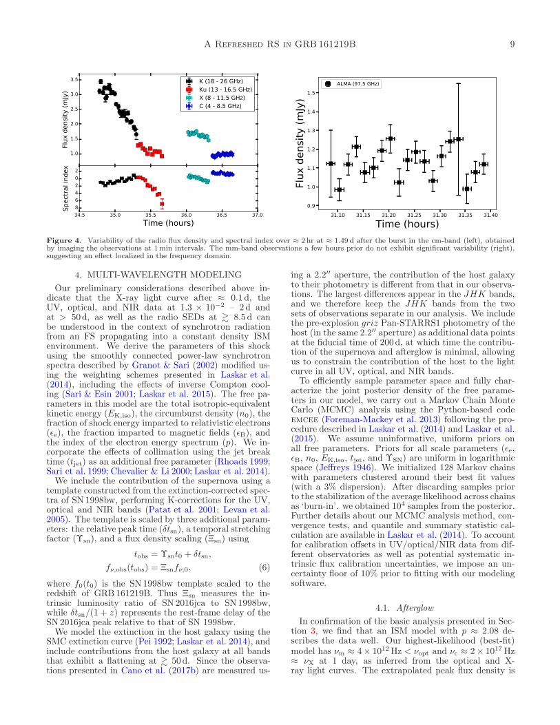
time resolution of minutes reveals another unexpectedvariability: the afterglow light curve exhibits rapidbrightening and fading within a single receiver base-band(2 GHz at K-band, 1 GHz otherwise) in the first fourepochs on time scales of minutes, while the spectral in-dex across base-bands within the same receiver tuningchanges rapidly (Figure 4). The mm-data do not exhibitcomparable levels of variability, with the scatter in thetime series being consistent with the mean uncertaintyof the measurements. Whereas variability on short timescales is a known characteristic of diffractive interstellarscintillation, such effects have not been observed at fre-quencies & 10GHz, as apparent for this event (Rickett1990). A detailed discussion of the cm-band variability is

presented in ALB18; for the purposes of our broad-bandanalysis, we use the time-averaged data for each epoch,together with the ALMA light curve to study the behav-ior of the afterglow in the cm and mm bands. The cm-band data in the first three epochs exhibit the greatestdegree of variability, and we do not include them whilecomputing the goodness of fit; however, they are impor-tant components for our final model, and we return todiscussing the full cm-band data set in Section 6.As the observed variability appears to decrease at

& 8.5 d, we attempt to derive the properties of the in-trinsic emission by fitting the radio SEDs after this time.As the precise fits depend on the data selected for fitting,the true uncertainty on the measured numbers below arelikely larger than those quoted, which are purely statis-tical.The radio SED at ≈ 8.5d exhibits a rising spectrum at

& 10GHz. Fitting the data above 10GHz with a brokenpower law,

Fν(ν) = Fb

[1

2

(ν

νb

)−yβ1

+1

2

(ν

νb

)−yβ2

]−1/y

, (4)

fixing β1 = 1/3, β2 = (1 − p)/2 ≈ −0.5, and y = 1.84−0.40p ≈ 1.0 (appropriate for νm; Granot & Sari 2002),yields νb = (9.2±1.0)×1010Hz with flux density, Fν,pk =0.508± 0.007mJy. The data at . 10GHz are in excessof the ν1/3 power law, while the spectrum at 16.5 d isrelatively flat and can be fit as a single power law withβ = −0.19 ± 0.03. We address both points together inSection 6.The SED at ≈ 24.5d exhibits a steep spectrum, β =

−1.1 ± 0.2 at ≈ 10–30GHz, which underpredicts theALMA observations at this time by a factor of ≈ 10.It is possible that the decrement in the VLA obser-vations at ν & 10GHz relative to lower frequencies isdue to phase decoherence, which systematically reducesthe observed flux32, as the data were acquired undermarginal weather conditions; we therefore remove thesedata also from our model fit. Fitting the cm-band dataat . 10GHz together with the ALMA observations, wefind νb = 9.4 ± 4.4GHz and Fν,pk = 0.49 ± 0.03mJy at≈ 24.5 d. The constancy of the peak flux density from8.5 d to 24.5 d identifies this break as νm and confirms thecircumburst medium as an ISM environment, for whichwe expect Fν,m ∝ t0; the observed decline rate of thisfrequency, αν,peak = −2.2± 0.5 is also consistent at 1.4σwith the expectation of ανm = −1.5.Projecting this frequency back to the optical bands at

earlier times with αν = −1.5, we expect the break tohave crossed R-band at ≈ 3× 10−2 d. Clear filter obser-vations calibrated to R-band from Terksol at 0.29d yieldfν,R = 0.56±0.01mJy (Mazaeva et al. 2016), in excellentagreement with νm ≈ νopt at this time. This is furtherconsistent with the subsequent decline rate and spectralindex in the optical bands (Section 3.1), confirming theoptical emission at & 3 × 10−2 d and radio observations

32 If the phase fluctuations induced by the atmosphere on agiven baseline can be approximated as a Gaussian random processwith zero mean and standard deviation, σ, then the expectation

of the interferometric visibility is 〈V 〉 = V e−σ2/2, where V is thetrue visibility. See Chapter 13 of Thompson et al. (2001) for aderivation.

8 Laskar et al.

109 1010 1011

Frequency (Hz)

10−1

100

Flux

den

sity (m

Jy) 0.5 d

109 1010 1011

Frequency (Hz)

10−1

100

Flux

den

sity (m

Jy) 1.4 d

109 1010 1011

Frequency (Hz)

10−1

100

Flux

den

sity (m

Jy) 3.4 d

109 1010 1011

Frequency (Hz)

10−1

100

Flux

den

sity (m

Jy) 4.5 d

109 1010 1011

Frequency (Hz)

10−1

100

Flux

den

sity (m

Jy) 8.5 d

109 1010 1011

Frequency (Hz)

10−1

100

Flux

den

sity (m

Jy) 16.5 d

109 1010 1011

Frequency (Hz)

10−1

100

Flux

den

sity (m

Jy) 24.5 d

109 1010 1011

Frequency (Hz)

10−1

100

Flux

den

sity (m

Jy) 79.0 d

109 1010 1011

Frequency (Hz)

10−1

100

Flux

den

sity (m

Jy) 158.5 d

Figure 3. Multi-frequency cm-band (VLA) and mm-band (ALMA) spectral energy distributions of the afterglow of 161219B from 0.5 dto ≈ 159 d, together with power law (16.5 d) and broken power law (8.5 d, 24.5 d, 79 d, and 158.5 d) fits (solid) to some of the observations(red points; see Section 3.2 for details). The radio SEDs exhibit unexpected variability in the cm-band (see also Figure 4).

at & 8.5 d as synchrotron emission from the FS. In theslow cooling regime, the afterglow peak flux density isgiven by,

Fν = 9.93(p+ 0.14)(1 + z)ǫ1/2B n

1/20 EK,iso,52d

−2L,28 mJy

∼ 50mJy (ǫB,−2n0)1/2

(1− ηradηrad

)Eγ,iso, (5)

for 161219B and p ≈ 2, where ηrad is the radiative ef-ficiency. Taking Fν,m ≈ 0.5mJy and assuming ηrad ≈

10%, we find n0 ≈ 6 × 10−4ǫ−1B,−2cm

−3, indicating a lowdensity environment.The ALMA light curve can be fit with a single power

law with α1 = −0.52± 0.02 from the first observation at1.3 d to the fourth epoch at ≈ 24.5 d. This is shallowerthan the expected decline rate of FS emission, and isbest described as a combination of two emitting compo-nents declining at different rates (Section 6). This best-fit power law over-predicts the flux density at the fifthepoch at 78.2 d by a factor of ≈ 3, which suggests a jetbreak has occurred between 24.5 and 78.2d, as indicatedby the X-ray observations (Section 3.1).The radio SED fades at all frequencies between 24.5 d

and 79.0 d, and the best fit broken power law modelat 79.0 d yields νb = 2.4 ± 0.8GHz with flux density

Fν,pk = 0.20 ± 0.02mJy (fixing the same parameters asat 24.5 d). The drop in peak flux further indicates a jetbreak has taken place between 24.5 d and 79.0 d. TheSED in the last epoch at 159.5 d can be fit either witha broken power law with β1 = 1/3 (fixed), β2 ≈ −0.5(fixed), νb = 7.9± 1.5GHz and Fν,pk = 0.12± 0.01mJy,or as a single power law with β = −0.8 ± 0.1. An in-crease in the break frequency νb with time is physicallyimplausible, and it is possible that the lowest frequencyobservations in this epoch have contribution from thehost galaxy. We discuss this epoch further in Section7.6.To summarize, the optical and X-ray light curves re-

quire a constant density environment with p ≈ 2. Themulti-band X-ray through radio observations of the af-terglow are consistent with a slow cooling FS (νm < νc)in an ISM environment with νm ≈ νopt at ≈ 3× 10−3 d,while the NIR to X-ray SED indicates νc ≈ νX for the du-ration of the X-ray observations. The UV spectral slopeis marginally steeper than that in the optical bands, in-dicating possible extinction in the host galaxy. The peakflux density of the FS is Fν,m ≈ 0.5mJy, implying thatthe optical and X-ray light curves prior to ≈ 3 × 10−2 dand radio SEDs prior to 8.5 d are dominated by emissionfrom a separate mechanism.

A Refreshed RS in GRB161219B 9

1.0

1.5

2.0

2.5

3.0

3.5

Flux density (mJy)

K (18 - 26 GHz)Ku (13 - 16.5 GHz)X (8 - 11.5 GHz)C (4 - 8.5 GHz)

34.5 35.0 35.5 36.0 36.5 37.0

Time (hours)

−8

−6

−4

−2

0

2

Spectral index

31.10 31.15 31.20 31.25 31.30 31.35 31.40

Time (hours)0.9

1.0

1.1

1.2

1.3

1.4

1.5

Flux

den

sity (m

Jy)

ALMA (97.5 GHz)

Figure 4. Variability of the radio flux density and spectral index over ≈ 2 hr at ≈ 1.49 d after the burst in the cm-band (left), obtainedby imaging the observations at 1min intervals. The mm-band observations a few hours prior do not exhibit significant variability (right),suggesting an effect localized in the frequency domain.

4. MULTI-WAVELENGTH MODELING

Our preliminary considerations described above in-dicate that the X-ray light curve after ≈ 0.1 d, theUV, optical, and NIR data at 1.3 × 10−2 – 2 d andat > 50d, as well as the radio SEDs at & 8.5 d canbe understood in the context of synchrotron radiationfrom an FS propagating into a constant density ISMenvironment. We derive the parameters of this shockusing the smoothly connected power-law synchrotronspectra described by Granot & Sari (2002) modified us-ing the weighting schemes presented in Laskar et al.(2014), including the effects of inverse Compton cool-ing (Sari & Esin 2001; Laskar et al. 2015). The free pa-rameters in this model are the total isotropic-equivalentkinetic energy (EK,iso), the circumburst density (n0), thefraction of shock energy imparted to relativistic electrons(ǫe), the fraction imparted to magnetic fields (ǫB), andthe index of the electron energy spectrum (p). We in-corporate the effects of collimation using the jet breaktime (tjet) as an additional free parameter (Rhoads 1999;Sari et al. 1999; Chevalier & Li 2000; Laskar et al. 2014).We include the contribution of the supernova using a

template constructed from the extinction-corrected spec-tra of SN1998bw, performing K-corrections for the UV,optical and NIR bands (Patat et al. 2001; Levan et al.2005). The template is scaled by three additional param-eters: the relative peak time (δtsn), a temporal stretchingfactor (Υsn), and a flux density scaling (Ξsn) using

tobs = Υsnt0 + δtsn,

fν,obs(tobs) = Ξsnfν,0, (6)

where f0(t0) is the SN1998bw template scaled to theredshift of GRB161219B. Thus Ξsn measures the in-trinsic luminosity ratio of SN2016jca to SN1998bw,while δtsn/(1 + z) represents the rest-frame delay of theSN2016jca peak relative to that of SN 1998bw.We model the extinction in the host galaxy using the

SMC extinction curve (Pei 1992; Laskar et al. 2014), andinclude contributions from the host galaxy at all bandsthat exhibit a flattening at & 50 d. Since the observa-tions presented in Cano et al. (2017b) are measured us-

ing a 2.2′′ aperture, the contribution of the host galaxyto their photometry is different from that in our observa-tions. The largest differences appear in the JHK bands,and we therefore keep the JHK bands from the twosets of observations separate in our analysis. We includethe pre-explosion griz Pan-STARRS1 photometry of thehost (in the same 2.2′′ aperture) as additional data pointsat the fiducial time of 200d, at which time the contribu-tion of the supernova and afterglow is minimal, allowingus to constrain the contribution of the host to the lightcurve in all UV, optical, and NIR bands.To efficiently sample parameter space and fully char-

acterize the joint posterior density of the free parame-ters in our model, we carry out a Markov Chain MonteCarlo (MCMC) analysis using the Python-based codeemcee (Foreman-Mackey et al. 2013) following the pro-cedure described in Laskar et al. (2014) and Laskar et al.(2015). We assume uninformative, uniform priors onall free parameters. Priors for all scale parameters (ǫe,ǫB, n0, EK,iso, tjet, and ΥSN) are uniform in logarithmicspace (Jeffreys 1946). We initialized 128 Markov chainswith parameters clustered around their best fit values(with a 3% dispersion). After discarding samples priorto the stabilization of the average likelihood across chainsas ‘burn-in’. we obtained 104 samples from the posterior.Further details about our MCMC analysis method, con-vergence tests, and quantile and summary statistic cal-culation are available in Laskar et al. (2014). To accountfor calibration offsets in UV/optical/NIR data from dif-ferent observatories as well as potential systematic in-trinsic flux calibration uncertainties, we impose an un-certainty floor of 10% prior to fitting with our modelingsoftware.

4.1. Afterglow

In confirmation of the basic analysis presented in Sec-tion 3, we find that an ISM model with p ≈ 2.08 de-scribes the data well. Our highest-likelihood (best-fit)model has νm ≈ 4× 1012Hz < νopt and νc ≈ 2× 1017 Hz≈ νX at 1 day, as inferred from the optical and X-ray light curves. The extrapolated peak flux density is

10 Laskar et al.

10−3 10−2 10−1 100 101 102

Time (days)

10−5

10−4

10−3

10−2

10−1

Flux

den

sity (m

Jy)

Swift-XRT

10−3 10−2 10−1 100 101 102Time (days)

10−7

10−5

10−3

10−1

101

Flux density (m

Jy)

O tical B-band x 53UVB x 52Optical u-band x 51UVU x 50

WHITE x 5−1UVW1 x 5−2UVM2 x 5−3UVW2 x 5−4

10−3 10−2 10−1 100 101 102

Time (day )10−6

10−5

10−4

10−3

10−2

10−1

100

101

102

Flux

den

ity (m

Jy)

Optical I-band x 53

Optical i'-band x 52

Optical R-band x 51

Optical r'-band x 50

Optical V-band x 5−1

UVV x 5−2

Optical g'-band x 5−3

10−3 10−2 10−1 100 101 102

Time (days)

10−5

10−4

10−3

10−2

10−1

100

101

Flux

den

si y

(mJy

)

UKIRT K-band x 53NIR K-band x 52NIR H-band x 51UKIRT H-band x 50

NIR J-band x 5−1

UKIRT J-band x 5−2

Optical z'-band x 5−3

100 101

Time (days)10−6

10−4

10−2

100

102

Flux

den

si y

(mJy

)

Radio K (19.0 GHz) x 5−3

Radio K (21 GHz) x 5−2

Radio K (23 GHz) x 5−1

Radio K (25 GHz) x 50

Radio Ka (30 GHz) x 51

Radio Ka (33.5 GHz) x 52

Millime er (ALMA) x 53

Millime er (ALMA) x 54

100 101 102Time (days)

10−5

10−3

10−1

101

103

Flux

den

sity (m

Jy)

Radi L (1.3 GHz) x 5−4

Radi L (1.6 GHz) x 5−3

Radi S (2.6 GHz) x 5−2

Radi S (3.4 GHz) x 5−1

Radi C (5 GHz) x 50

Radi C (7 GHz) x 51

Radi X (8.5 GHz) x 52

Radi X (11 GHz) x 53

Radi Ku (13.4 GHz) x 54

Radi Ku (15.9 GHz) x 55

Figure 5. X-ray (top left), UV (top right), optical (center left), NIR (center right), and radio (bottom) light curves ofGRB161219B/SN2016jca, together with an FS ISM model including contributions from the supernova light (solid lines). We show adecomposition of the Swift/w2-band, optical g′-band, and optical z′-band light curves into FS (dashed) and supernova (dash-dotted) com-ponents. Data represented by open symbols are not included in the model fit. The JHK photometry from GROND, NOT, and GTC wasreported in a 2.2′′ aperture and does not include the full light of the host; these bands are therefore treated separately from the UKIRTphotometry, which does include all contributions from the host (Section 4). This FS-only model over-predicts the X-ray data at . 0.1 d,and under-predicts the optical observations at . 3× 10−3 d as well as the radio observations at . 8.5 d; both deficiencies are overcome inthe refreshed RS model presented in Figure 10.

A Refreshed RS in GRB161219B 11

Fν,m ≈ 1mJy. The peak of the rounded spectrum33 is

then Fν,pk = 2−1/yFν,m ≈ 0.5mJy, consistent with theradio SEDs and the optical observations at ≈ 3× 10−2 d(Section 3.2). The afterglow remains in the slow coolingregime for the duration of the observations.This model also requires a jet break at tjet ≈ 32 d,

corresponding to an opening angle of ≈ 13 (Sari et al.1999). The resulting beaming-corrected kinetic and γ-ray energies are EK ≈ 1.3 × 1050 erg and Eγ ≈ 4.9 ×

1048 erg, respectively. The corresponding radiative ef-ficiency is extremely low, η ≈ 4% (independent of thebeaming angle). We discuss this further in Section 6.This break time is later than derived from fitting the X-ray light curve alone (Section 3.1), owing to the steeperpost-break decline rate in the physical model comparedto the simple power law fits of the X-ray light curve.The resulting model matches the X-ray data at & 0.1 dfairly well (Figure 5). We note the time of the jetbreak is partly driven by the ALMA light curve, whichdeclines as α = −1.5 ± 0.3 between 24.5 and 78.2 d,steeper than the expected value of ≈ −0.8 for the order-ing νm < νALMA < νc and a spherical, adiabatic shock,as also discussed in Section 3.2. The resulting modellight curve matches the ALMA flux density in the fi-nal 3 epochs, but underpredicts the mm- and cm-bandobservations before ≈ 8.5 d (Figure 6). The parametersfor the best fit model, together with the median and 68%credible intervals from the MCMC analysis, are providedin Table 8 and histograms of the marginalized posteriordensity are presented Figure 7. We note that νa is notconstrained by the data, resulting in some degeneraciesbetween the physical parameters (Figure 8).

4.2. Supernova

The supernova (SN 2016jca) associated with this bursthas previously been studied by Ashall et al. (2017) andCano et al. (2017b), who consider both magnetar andradioactive decay models for powering the SN lightcurve. Ashall et al. (2017) argue for the magnetar modelwith an ejecta mass of Msn,ej ≈ 8M⊙, despite thehigh isotropic-equivalent ejecta kinetic energy required,Esn,K,iso ≈ 5.4× 1054 erg. Their afterglow model used toderive the SN light curve requires p < 2, while the largejet opening angle they infer, θjet ≈ 40, is based on an as-sumed circumburst density of n0 ≈ 1cm−3, over 3 ordersof magnitude larger than the value obtained here frommulti-wavelength modeling. Cano et al. (2017b) derive alower ejecta mass, Msn,ej = 5.8 ± 0.3M⊙, and a similarejecta kinetic energy, Esn,K,iso = (5.1 ± 0.8) × 1054 erg.Under the assumption that the SN light curve is pow-ered by radioactive decay of 51Ni, they find a Nickelmass of MNi = 0.22 ± 0.08M⊙, and γ-ray opacity, κγ ≈

0.034 cm2 g−1. Our method, which assumes the samecolor evolution as the template, yields a stretch factor ofΥsn ≈ 0.8 and a flux scale factor34 of Ξsn ≈ 0.8, within≈ 1σ of the correlation between these parameters derivedby Cano (2014). Whereas our method does not allow us

33 Here y = 1.84−0.40p ≈ 1.0 is the smoothness of the νm break.34 These correspond to the parameters k and s of Cano (2014),

respectively. We use different symbols in this work to avoid con-fusion with the the ejecta Lorentz factor distribution (equation 7)and the circumburst medium density profile index.

Table 8Results of multi-wavelength modeling

Parameter Best-fit MCMC

Forward Shock

p 2.08 2.079+0.009−0.006

ǫe 0.93 0.89+0.05−0.07

ǫB 5.1× 10−2 (5.8+5.4−3.0)× 10−2

n0(cm−3) 3.6× 10−4 (3.2+1.4−1.2)× 10−4

EK,iso,52 (erg) 0.47 0.46+0.14−0.09

tjet (d) 31.5 33.0+1.5−1.4

θjet (deg) 13.5 13.44 ± 0.35

AV (mag) 3.0× 10−2 (2.1+2.0−2.1)× 10−2

EK (erg) 1.3× 1050 (1.27+0.36−0.25)× 1050

Prompt Emission

Eγ,iso (1.8± 0.4)× 1050 . . .

Eγ (erg) 4.9× 1048 (4.9± 1.9)× 1048

ηrad 3.7% . . .

SN 2016jca

δtsn,peak (d) −3.7 −4.10+0.80−0.96

Υ 0.83 0.84± 0.04

Ξf 0.73 0.76± 0.02

Mean host contribution (µJy)

uw2 1.64 1.57± 0.34

um2 1.48 1.12+0.30−0.51

uw1 2.35 2.39± 0.27

uwh 5.03 4.90± 0.35

uvu 3.61 3.26± 0.39

u′ 2.92 2.77+0.59−0.81

uvb 8.35 8.03+0.38−0.69

B 3.89 3.64± 0.25

g′ 9.58 9.28± 0.27

uvv 6.61 5.32± 0.88

V 15.3 14.0± 0.8

r′ 13.2 12.8± 0.6

R 11.9 10.6± 1.0

i′ 17.1 16.4± 0.6

I 14.1 13.4± 1.0

z′ 20.2 19.6± 0.65

UKIRT-J 30.6 31.5± 2.1

J 19.2 17.3± 1.2

UKIRT-H 28.7 29.3± 2.5

H 19.1 18.5± 1.2

K 17.3 18.4± 2.0

UKIRT-K 34.5 37.5± 2.5

5GHz 60.2 52.0± 16.4

7.4GHz 42.0 41.2± 13.2

12 Laskar et al.

109 1010 1011

Frequency (Hz)

10−1

100

Flux

den

sity (m

Jy) 0.5 d

109 1010 1011

Frequency (Hz)

10−1

100

Flux

den

sity (m

Jy) 1.4 d

109 1010 1011

Frequency (Hz)

10−1

100

Flux

den

sity (m

Jy) 3.4 d

109 1010 1011

Frequency (Hz)

10−1

100

Flux

den

sity (m

Jy) 4.5 d

109 1010 1011

Frequency (Hz)

10−1

100

Flux

den

sity (m

Jy) 8.5 d

109 1010 1011

Frequency (Hz)

10−1

100

Flux

den

sity (m

Jy) 16.5 d

109 1010 1011

Frequency (Hz)

10−1

100

Flux

den

sity (m

Jy) 24.5 d

109 1010 1011

Frequency (Hz)

10−1

100

Flux

den

sity (m

Jy) 79.0 d

109 1010 1011

Frequency (Hz)

10−1

100

Flux

den

sity (m

Jy) 158.5 d

Figure 6. Multi-frequency cm-band (VLA) and mm-band (ALMA) spectral energy distributions of the afterglow of 161219B, togetherwith a forward shock ISM model (solid lines; Section 4). The red shaded regions represent the expected variability due to scintillation.This FS-only model under-predicts the radio observations at . 8.5d, and requires an additional component (Section 6 and Figure 12).

to derive specific physical parameters of SN2016jca, ourresults are broadly consistent with those of Cano et al.(2017b), who find (frequency-dependent) stretch factorsof Υsn ≈0.6–0.9 and Ξsn ≈0.7–0.8.

4.3. Host galaxy

We derive an SED for the host galaxy using five ofthe six narrow-band UVOT filters35, together with thepre-explosion PS1 grizy host photometry (Cano et al.2017b) and our JHK data (Figure 9). We fit a setof galaxy templates from Bruzual & Charlot (2003) us-ing FAST (Kriek et al. 2009), assuming an exponentiallydeclining star-formation history (τ -model), a Chabrier(2003) IMF, and a stellar metallicity of Z = 0.008 (0.4 so-lar, corresponding to the value for the host obtained fromHα and emission line diagnostics; Cano et al. 2017b).Whereas the extinction and τ are particularly suscepti-ble to systematic photometric uncertainties in the Swiftphotometry and are poorly constrained by the weak UVdetections of the host, the stellar mass is well determined,log(M∗/M⊙) = 8.92+0.04

−0.02. We derive a stellar popula-

35 Photometry in the UVOT v-band is most significantly affectedby diffracted light from the nearby star, and is less reliable thanin the other bands at late times. We therefore exclude this bandfrom the SED fit.

tion age, log t0 = 9.0+0.2−0.1, τ ≈ 0.3Gyr, rest-frame ex-

tinction, AV = 0.6+0.2−0.6mag, and current star-formation

rate SFR = 0.19+0.02−0.16M⊙ yr−1. These values are similar

to those derived by Cano et al. (2017b) using the PS1photometry alone. The derived stellar mass is compa-rable to the mean stellar mass of GRB hosts at z . 1(log(M∗/M⊙) = 9.25+0.19

−0.23; Levesque et al. 2010). On

the other hand, the specific SFR, log [sSFR/Gyr−1] ≈

−0.65 appears an order of magnitude lower than the me-dian sSFR of GRB hosts at z . 1 (log [sSFR/Gyr−1] ≈0.3; Levesque et al. 2010). The possibility that the GRBoccurred in an extreme star-forming region within anotherwise low sSFR host is disfavored by HST spec-troscopy of the supernova site (Cano et al. 2017b). Dustextinction may impact the derived SFR by extinguishingthe light from young stars, especially in an edge-on sys-tem like the host of GRB 161219B; however, we derive alow extinction from afterglow modeling, consistent withthe host SED fits. Since long-duration GRBs are typi-cally associated with regions of the most intense star for-mation in their hosts (Bloom et al. 2002; Fruchter et al.2006; Svensson et al. 2010; Blanchard et al. 2016), thelack of evidence for strong star-formation activity at theGRB site is puzzling.

A Refreshed RS in GRB161219B 13

1006×10−1 7×10−1 8×10−1 9×10−10

1.0×104

2.0×104

3.0×104

4.0×104

5.0×104εe

10−2 10−10

1.0×104

2.0×104

3.0×104

4.0×104 εB

10−40

1.0×104

2.0×104

3.0×104

4.0×104 n0

1000

1.0×104

2.0×104

3.0×104

4.0×104 EK, iso, 52

0.000 0.015 0.030 0.045 0.0600

2.0×104

4.0×104

6.0×104 AV

2.070 2.085 2.100 2.1150

1.0×104

2.0×104

3.0×104

4.0×104

5.0×104 p

28 30 32 34 36 38 400

1.0×104

2.0×104

3.0×104

4.0×104

5.0×104tjet

11.2 12.0 12.8 13.6 14.4 15.20

1.0×104

2.0×104

3.0×104

4.0×104θjet

1000

1.0×104

2.0×104

3.0×104

4.0×104 EK, 50

−9.0 −7.5 −6.0 −4.5 −3.0 −1.50

1.0×104

2.0×104

3.0×104

4.0×104 δtsn

0.72 0.78 0.84 0.90 0.96 1.020

1.0×104

2.0×104

3.0×104

4.0×104 Υsn

0.69 0.72 0.75 0.78 0.81 0.840

1.0×104

2.0×104

3.0×104

4.0×104

5.0×104 Ξsn

Figure 7. Posterior probability density functions for the physicalparameters for GRB161219B and the light curve of SN 2016jca.

5. ENERGY INJECTION

The optical and X-ray light curves exhibit an unusualachromatic break at ≈ 0.1 d, which cannot be explainedin the standard synchrotron framework. Furthermore,the model described in Section 4 over-predicts the X-ray light curve before ≈ 0.1 d (Figure 5). One of thesimplest means to obtain a flatter light curve at earliertimes is through the injection of energy into the forwardshock due to extended activity of the central engine,

−4.0 −3.8 −3.6 −3.4 −3.2log(n0)

−0.5−0.4−0.3−0.2−0.10.00.10.2

log(E K

,iso,

52)

−0.25−0.20−0.15−0.10−0.05log(εe)

−0.5−0.4−0.3−0.2−0.10.00.10.2

log(E K

,iso,

52)

−0.25−0.20−0.15−0.10−0.05log(εe)

−4.0

−3.8

−3.6

−3.4

−3.2

log(n 0)

−2.5 −2.0 −1.5 −1.0 −0.5log(εB)

−0.5−0.4−0.3−0.2−0.10.00.10.2

log(E K

,iso,

52)

−2.5 −2.0 −1.5 −1.0 −0.5log(εB)

−4.0

−3.8

−3.6

−3.4

−3.2

log(n 0)

−2.5 −2.0 −1.5 −1.0 −0.5log(εB)

−0.25

−0.20

−0.15

−0.10

−0.05

log(ε e)

Figure 8. 1σ (red), 2σ (green), and 3σ (black) contours for corre-lations between the physical parameters, EK,iso, n0, ǫe, and ǫB forGRB161219B from Monte Carlo simulations. We have restrictedǫe + ǫB < 1. See the on line version of this Figure for additionalcorrelation plots.

100

Wavelength (μm)

10−14

10−13

λFλ (ergs

−1cm

−2)

Figure 9. SED of the host of GRB 161219B derived from multi-wavelength modeling (Section 4), together with a best-fit modelfrom Bruzual & Charlot (2003).

the deceleration of a Poynting flux dominated outflow,or stratified ejecta with additional energy available atlower Lorentz factors (Dai & Lu 1998; Rees & Meszaros1998; Kumar & Panaitescu 2000; Sari & Meszaros 2000;Zhang & Meszaros 2001, 2002; Granot & Kumar 2006;Zhang et al. 2006; Dall’Osso et al. 2011; Uhm et al.2012). The effect on the FS is a gradual increase inthe effective shock energy with time, E ∝ tm ∝ t1−q,where −q ≡ m−1 is the power law index of the injectionluminosity, L ∝ t−q (Zhang et al. 2006). For energy in-jection due to accumulation from a distribution of ejecta

14 Laskar et al.

Lorentz factors, the corresponding ejecta energy distri-bution is given by E(> Γ) ∝ Γ1−s, with

s =(7m+ 3)− k(2m+ 1)

(3 − k)−m, (7)

where the external density profile as a function of ra-dius, R, is assumed to follow the general36 power lawform, ρ = AR−k. During this process, the FS Lorentzfactor, shock radius, and post-shock magnetic field allevolve more slowly than the standard relativistic solu-tion (Blandford & McKee 1976; Sari & Meszaros 2000;Zhang et al. 2006),

∂ ln Γ

∂ ln t= −

q + 2− k

2(4− k)= −

3− k

7 + s− k,

∂ lnR

∂ ln t=

2− q

4− k=

1 + s

7 + s− 2k,

∂ lnB

∂ ln t= −

q + k + 2− kq

2(4− k)= −

6 + ks− k

2(7 + s− 2k), (8)

with s and q related by

s =10− 3k − 7q + 2kq

2 + q − k,

q =10− 2s− 3k + ks

7 + s− 2k. (9)

The standard hydrodynamic evolution in the absence ofenergy injection can be recovered by setting m = 0, s = 1or q = 1 in the above expressions (e.g., Gao et al. 2013).In our best-fit model, νX < νc at . 0.1 d, whereupon

m = (4αX + 3p − 3)/(p + 3) = 0.35 ± 0.09 using αX =−0.37± 0.09 (Section 3.1), which implies s ≈ 2 for k = 0(equation 7) in the massive ejecta model. No theoreticalmodels yet exist of the expected distribution of ejectaLorentz factors, and in fact the distribution need notfollow a power law. However, our observations of energyinjection in this event add to the growing collection of ameasurement of s in GRB jets (Laskar et al. 2015).We note that the forward shock cooling frequency,

νc,f ∝ E−1/2t−1/2 ∝ t−(m+1)/2 ∼ t−0.65. Thus, in ourmodel νc,f evolves from ≈ 3 × 1018Hz to ≈ 7 × 1017Hzbetween the end of the flare at ≈ 0.01d and the end ofenergy injection at ≈ 0.1 d. The presence of νc,f withinthe Swift X-ray band explains the observed X-ray spec-tral index, βX ≈ −0.86, which is intermediate between(1− p)/2 ≈ −0.54 and −p/2 ≈ −1.04.Since the peak flux density is ≈ 0.5mJy and fν,m is

constant in an ISM environment, a measured flux densitygreater than this value at any frequency and time cannotbe explained by FS emission. Thus, as we previouslyargued, the optical light curve before ≈ 3 × 10−2 d andthe radio SEDs before ≈ 8.5 d must be dominated by adistinct emission component. Whereas energy injectioncan explain the relatively flat X-ray light curve before≈ 0.1 d, adding this to our model further worsens the fitto the optical light curves at that time. We address bothconcerns in the next section.

6. REVERSE SHOCK

36 We keep the discussion here general for completeness, andspecialize to the ISM (k = 0) case later.

During the process of energy injection, a reverseshock mediates the transfer of energy from the ejectainto the FS. This RS, which is Newtonian or mildlyrelativistic, propagates for the period of the injec-tion and (by definition) crosses the ejecta at the time(tE) when energy injection terminates (Rees & Meszaros1998; Kumar & Piran 2000; Zhang et al. 2003). Such a“long-lasting” RS propagating into the ejecta releasedduring the GRB may produce detectable synchrotronradiation (Sari & Meszaros 2000; Uhm 2011). We nowshow that such an RS can reproduce the observed ex-cess in both the optical light curves at . 3× 10−2 d andthe radio SEDs at . 8.5 d, beginning first with the theo-retical model (Section 6.1), followed by the results fromour data (Section 6.2), and consistency checks betweentheory and observations (Section 6.3).

6.1. Energy injection RS – theoretical prescription

A detailed calculation of the hydrodynamics of thedouble shock system requires numerical simulations orsemi-analytic modeling. Here, we follow previous an-alytic work Sari & Meszaros (2000); Uhm (2011) andmake the simplifying assumption that the pressure be-hind the RS is equal to that at the FS, P ∝ Γ2ρ (however,see Uhm et al. 2012 for a discussion of situations wherethis assumption is relaxed). The characteristic frequency,cooling frequency, and peak flux density of the radiationfrom the RS and FS are then related during the shockcrossing (t < tE) by

νm,r

νm,f∼ Γ−2RBR

2e ,

νc,rνc,f

∼ R−3B

(1 + Yf

1 + Yr

)2

,

Fν,m,r

Fν,m,f∼ ΓRB, (10)

where Γ is the Lorentz factor of the FS, RB ≡

(ǫB,r/ǫB,f)1/2 is the ejecta magnetization, Yr and Yf are

the Compton Y -parameters for the RS and FS, respec-tively, and Re ≡ ǫe,r/ǫe,f , with ǫe ≡ (p − 2)ǫe/(p − 1)(Zhang et al. 2006). We assume the same value of p forboth the RS and FS, so that Re = ǫe,r/ǫe,f. As for theFS, we assume that the microphysical parameters of theRS (and hence Re and RB) remain constant with time.Thus, the RS spectral parameters are directly propor-tional to those of the FS during shock crossing:

νm,r ∝ Γ−2νm,f ,

νc,r ∝ νc,f ,

Fν,m,r ∝ ΓFν,m,f . (11)

The number of electrons swept up by the FS (prior tothe jet break) is given by Ne,f ∝ R3ρ ∝ R3−k. Sinceνm,f ∝ Γγ2

eB, νc,f ∝ Γ−1B−3t−2, and Fν,m,f ∝ Ne,fBΓ,while the minimum Lorentz factor of accelerated elec-trons, γe ∝ Γ, the spectral parameters of the FS at t < tE

A Refreshed RS in GRB161219B 15

are (Zhang et al. 2006),

∂ ln νm,f

∂ ln t= −

q + 2

2,

∂ ln νc,f∂ ln t

=(3k − 4)(2− q)

2(4− k),

∂ lnFν,m,f

∂ ln t=

3kq − 4k − 8q + 8

2(4− k). (12)

These equations reduce to the standard results in theabsence of energy injection (q = 1), and can also berecovered by setting E ∝ tm in the expressions given byGranot & Sari (2002). Combining equations 11 and 12,the spectral parameters of the RS at t < tE are,

∂ ln νm,r

∂ ln t= −

2q − kq + 4

2(4− k),

∂ ln νc,r∂ ln t

=(3k − 4)(2− q)

2(4− k),

∂ lnFν,m,r

∂ ln t=

3(kq − k − 3q + 2)

2(4− k), (13)

which yield the expressions of Sari & Meszaros (2000) fork = 0.The evolution of the RS self-absorption frequency dur-

ing energy injection is more complex, and depends on therelative ordering of νa,r, νm,r, and νc,r. When both theRS and FS are in the slow cooling regime (νm,r < νc,rand νm,f < νc,f), we expect νa,r ∝ Γ8/5νa,f at t < tE(Sari & Meszaros 2000), so that

∂ ln νm,r

∂ ln t= −

8

5

[q + 2− k

2(4− k)

]+

∂ ln νm,f

∂ ln t(14)

which equals − q+25 (slower than the evolution of νm,r) for

the ISM case. We later show (Section 6.2) that νm,r ≈νa,r at ≈ 1.4 d, so that νa,r does not affect the light curveat any observed frequency prior to the end of energyinjection at tE. We therefore ignore self-absorption inthe RS prior to tE.After injection ends, the residual RS spectrum fades

according to the standard RS prescription (Kobayashi2000; Zou et al. 2005). The evolution of νa,r, νm,r, νc,r,and Fν,m,r at t > tE depend on whether the RS wasNewtonian or relativistic. For a relativistic RS, no ad-ditional parameters are necessary, while for a Newto-nian RS, we follow Kobayashi & Sari (2000) in param-eterizing the evolution of the ejecta Lorentz factor asΓ ∝ R−g. Since the shocked ejecta lag the FS and theFS Lorentz factor evolves with radius as t(3−k)/2, we ex-pect g > (3− k)/2. On the other hand, the fluid Lorentzfactor in the adiabatic Blandford & McKee (1976) so-lution evolves as γf ∝ t(2k−7)/2 (Wu et al. 2003); sincea Newtonian RS does not decelerate the ejecta effec-tively, its Lorentz factor is expected to evolve with ra-dius slower than the Blandford-McKee solution. Thus(3 − k)/2 ≤ g ≤ (2k − 7)/2, or 3/2 ≤ g ≤ −7/2 for theISM environment and 1/2 ≤ g ≤ 3/2 in the wind case.Using numerical simulations, Kobayashi & Sari (2000)

found g ≈ 2 for a standard Newtonian RS not associ-ated with energy injection in the ISM environment, andg ≈ 3 for a relativistic RS. Recent observations of ra-dio afterglows have constrained g ≈ 5 for GRB130427A

(Laskar et al. 2013; Perley et al. 2014) in the wind en-vironment (outside the canonical range) and g ≈ 2for GRB160509A in an ISM environment (Laskar et al.2016). We consider both the relativistic and Newto-nian prescriptions for evolution at t > tE in our anal-ysis, discussing self-consistency in Section 6.3. Followingthe jet break, the evolution of Fν,m,r steepens furtherby a factor of Γ2 due to geometric effects (Rhoads 1999;De Colle et al. 2012; Granot & Piran 2012; Laskar et al.2016) and we include this in our modeling.

6.2. Energy injection RS – observational constraints

A detailed study of spectro-temporal variability in theradio afterglow in our companion paper, ALB18, indi-cates the variability peaks at 10–30GHz at t . 8.5 d,but is minimal at lower frequencies and in the ALMAbands (Figure 4). We therefore anchor our RS model tothe LSC bands at cm wavelengths (1 ∼ 10GHz) and tothe ALMA bands at ≈ 100GHz. From the observed cm-to mm-band SEDs (Figure 6), we require the RS spec-tral peak, νm,r ≈ 10GHz at 1.4 d, with Fν,m,r ≈ 4mJy.Since the flux density in the first epoch at ≈ 0.5 d is. 1mJy at all bands and the RS light curves rise belowνa,r and fade below νm,r, we expect νa,r to be located at1–10GHz at 0.5 and 1.4 d to explain the observed bright-ening from between the first two epochs. Since the mm-band data are brighter than the prediction from the FSat both 1.4 d and 3.4 d, the RS must contribute some fluxat those frequencies, and hence νc,r & 100GHz at 3.4 d.On the other hand, we require νc,r . νopt at ≈ 10−2 dso as to not over-predict the UV/optical light curves be-fore ≈ 0.1 d, implying ∂ ln νc,r/∂ ln t & −2. Thus the RSbreak frequencies should be ordered as νa,r . νm,r < νc,rat ≈ 1.4 d. This is challenging to achieve with highlyrelativistic RS models, for which νc,r ∝ t−15/8 onlymarginally satisfies the above condition. Upon detailedconsideration, no relativistic RS models are able to re-produce the observations, and we focus in the rest of thissection on models involving Newtonian or mildly rela-tivistic shocks.From the energy injection model in Section 5, m ≈

0.35, implying q ≈ 0.65 in an ISM environment. For this

value of q, the RS spectrum evolves as∂ ln νm,r

∂ ln t ≈ −0.66,∂ ln νc,r∂ ln t ≈ −0.68, and

∂ lnFν,m,r

∂ ln t ≈ 0.02 at t < tE. Thusthe RS peak flux is approximately constant during shockcrossing. Evolution after shock crossing depends on thevalue of g.Under this spectral evolution and the observational

constraints described above, we find that an RS modelwith g ≈ 2.8, tE ≈ 0.25 d, νc,r(tE) ≈ 1.2 × 1015 Hz,νm,r(tE) ≈ 9.4 × 1010 Hz, νa,r(tE) ≈ 5.9 × 1010Hz, andFν,m,r(tE) ≈ 22mJy fits the early optical and X-ray datawell (Figure 10). This value of g is intermediate be-tween the values expected for a Newtonian (g ≈ 2.2) andrelativistic RS (g ≈ 3) for the case of no energy injec-tion. In this model, the X-ray light curve is dominatedby the FS at all times, with the suppression prior to0.25d arising from energy injection with m ≈ 0.35. TheUV/optical/NIR light curves are dominated by the FS af-ter the end of energy injection at≈ 0.25d and exhibit sig-nificant contribution from the RS arising from injectionprocess prior to this time (Figure 11). The radio SEDs at≈ 1.4, 3.4, 4.5, and 8.5 d are well matched by the same

16 Laskar et al.

10-3 10-2 10-1 100 101 102

Time (days)

10-5

10-4

10-3

10-2

10-1

Flux density (mJy)

Swift-XRT

10-3 10-2 10-1 100 101 102

Time (days)

10-7

10-6

10-5

10-4

10-3

10-2

10-1

100

101

102

Flux density (mJy)

Optical B-band x 53

UVB x 52

Optical u-band x 51

UVU x 50

WHITE x 5−1

UVW1 x 5−2

UVM2 x 5−3

UVW2 x 5−4

10-3 10-2 10-1 100 101 102

Time (days)

10-6

10-5

10-4

10-3

10-2

10-1

100

101

102

Flux density (mJy)

Optical I-band x 53

Optical i'-band x 52

Optical R-band x 51

Optical r'-band x 50

Optical V-band x 5−1

UVV x 5−2

Optical g'-band x 5−3

10-3 10-2 10-1 100 101 102

Time (days)

10-5

10-4

10-3

10-2

10-1

100

101

Flux d

ensi

ty (m

Jy)

UKIRT K-band x 53

NIR K-band x 52

NIR H-band x 51

UKIRT H-band x 50

NIR J-band x 5−1

UKIRT J-band x 5−2

Optical z'-band x 5−3

100 101

Time (days)

10-6

10-5

10-4

10-3

10-2

10-1

100

101

102

103

Flux density (mJy)

Radio K (19.0 GHz) x 5−3

Radio K (21 GHz) x 5−2

Radio K (23 GHz) x 5−1

Radio K (25 GHz) x 50

Radio Ka (30 GHz) x 51

Radio Ka (33.5 GHz) x 52

Millimeter (ALMA) x 53

Millimeter (ALMA) x 54

100 101 102

Time (days)

10-6

10-5

10-4

10-3

10-2

10-1

100

101

102

103

104

Flux density (mJy)

Radio L (1.3 GHz) x 5−4

Radio L (1.6 GHz) x 5−3

Radio S (2.6 GHz) x 5−2

Radio S (3.4 GHz) x 5−1

Radio C (5 GHz) x 50

Radio C (7 GHz) x 51

Radio X (8.5 GHz) x 52

Radio X (11 GHz) x 53

Radio Ku (13.4 GHz) x 54

Radio Ku (15.9 GHz) x 55

Figure 10. X-ray (top left), UV (top right), optical (center left), NIR (center right), and radio (bottom) light curves ofGRB161219B/SN2016jca, together with a full FS+RS model with energy injection (solid lines). We show a decomposition of the X-ray, Swift/w2-band, optical g′-band, optical z′-band, 19GHz and 1.3GHz light curves into FS (with energy injection; dashed), refreshedRS (dotted) and supernova (dash-dotted) components. The combined model overcomes the deficiencies of the FS-only model (withoutenergy injection; Section 4; Figures 5 and 6), and explains the overall behavior of the light curves at all 41 observing frequencies over 5orders of magnitude in time. Residual differences in the 10–30GHz VLA light curves are likely related to the rapid cm-band variabilityobserved for this event (Section 3.2). See Figure 17 in the appendix for a combined plot showing all 41 observing frequencies.

A Refreshed RS in GRB161219B 17

1014 1015 1016 1017 1018

Frequency (Hz)10 5

10 4

10 3

10 2

10 1

100

Flux density (mJy)

0.009 d0.29 d1.5 d

Figure 11. NIR to X-ray spectral energy distributions of theafterglow of GRB161219B at 9 × 10−3 d (blue), 0.29 d (orange)and 1.5 d (green), together with the best-fit synchrotron model tothe entire multi-band data set (Section 4; solid lines). The dipin the UV is the combined effect of extinction in the Galaxy andin the host. The optical data have been interpolated using theaverage UV light curve (Table 7); the contribution of the host hasbeen removed. The dashed lines represent the FS model withoutphotoelectric absorption or optical extinction; the peak at ≈ 3 ×1015 Hz in the first epoch is νm, and the break at ≈ 2 × 1017 Hzin the later epochs is νc. The SED at 9 × 10−3 d is dominated bythe RS in the optical (dotted) and the FS in the X-rays (Section6); RS contribution at later times is negligible in the optical andX-rays. The slight discrepancy in the X-ray SED in the first twoepochs may arise from Klein-Nishina corrections to the light curveabove νc (Section 7.5).

RS, propagated to the times of the radio observations(Figure 12). Whereas the model does over-predict the18–26GHz observations at 0.5 d, we caution that thesefrequencies also exhibit the greatest cm-band variabilitybefore ≈ 8.5 d, possibly due to extreme interstellar scin-tillation (ALB18). The large scatter in flux density ob-served between individual frequencies in the SED furthercomplicates the comparison against the model predictionat this time. Finally, the model also explains the excessin the ALMA light curve37 at . 3.4 days (Figure 13).

6.3. Energy injection RS – self-consistency with FS

If the excess flux density in the early optical and radioobservations of GRB161219B arises from an RS mediat-ing energy injection, we expect the parameters of the RSand FS to be related at the time of cessation of the injec-tion (tE ≈ 0.25d). From the FS parameters derived frommulti-wavelength modeling (Table 8), the Lorentz factorof the FS is Γ(tE) ≡ ΓE ≈ 22.7 (Blandford & McKee1977). We present a comparison between the observedRS parameters and the values expected by scaling theFS parameters by ΓE in Table 9. We find the peak fluxdensity to match within 5%(!), suggesting that the RSis not magnetized relative to the FS. The characteris-tic frequencies also agree upon scaling to within 50%, astronger match than previously obtained for the Newto-nian RS detected in GRB130427A (Laskar et al. 2013;Perley et al. 2014). Whereas the scaled ratio of the self-

absorption frequencies νa,r/Γ8/5E νa,f is too large by a fac-

37 See Figure 17 in the appendix for a combined plot showingall 41 observing frequencies.

tor of ≈ 20, we note that νa,f is not well constrained,being below the radio band at all times.The ratio of the cooling frequencies νc,f/νc,r ≡ Qc,fr ≈

3.6 × 102 is larger than expected, which is difficult toexplain if RB ≈ 1. Since νc,r does not have a strongobservational signature being hidden inside the FS spec-trum, it could be higher by a factor of several; however,increasing νc,r(tE) beyond ≈ 1016Hz does begin to affectthe X-ray light curve at 10−2 to 2 × 10−1 d. Anotherpossibility is that the Compton Y -parameter of the RSis higher than the FS. In the regime ǫe ≫ ǫB, we expectY ≈

√ηYǫe/ǫB, where ηY = (νc/νm)

−(p−2)/2. Since thisratio is lower than the corresponding ratio for the FS, weexpect Yr . Yf , and thus inverse Compton cooling cannotexplain the observed high ratio of νc,f to νc,r. The thirdoption is that νc,f is lower than predicted from the model.A reduced value of νc,f would require the spectral indexabove νc,f to be shallower than −p/2 in order to continueto match the X-ray light curve. Such a flatter spectrumis indeed afforded by the Klein-Nishina correction to thesynchrotron spectrum. We discuss this further in Sec-tion 7.5 and Appendix A. We note that recent numericalwork suggests the analytical relations over-predict theRS flux by factors of a few to ≈ 10 (Nakar & Piran 2004;Harrison & Kobayashi 2013); thus, it is possible that theequivalence between these quantities derived above mayarise from a coincidence, and that the ejecta are mag-netized at the level RB ≈ 5–10. Since νc,f/νc,r ∝ R3

Bis strongly dependent on RB, even a slight RS magne-tization (say RB ≈ 2, which may be feasible given theuncertainties in the RS parameters), could alleviate theproblem. Thus, a combination of a higher value of νc,r,a lower value of νc,f , or slight ejecta magnetization mayexplain the apparent discrepancy.The observed strong RS signature in GRB161219B can

be used to place constraints on the circumburst density.The UV/optical light curves prior to the end of energyinjection at ≈ 0.25 suggest νc,r & 1015Hz at this time.Combining equation 13 with the expression for FS cool-ing frequency from Granot & Sari (2002),

νc,f = 6.37× 1013(p− 0.46)e−1.16p(1 + z)−1/2

× ǫ−3/2B n−1

0 E−1/2K,iso,52(1 + Yf)

−2t−1/2d Hz

≈ 5× 1013ǫ−3/2B,−1n

−10 Hz

∼ R3Bνc,r (15)

at the redshift of GRB161219B for p ≈ 2.1, EK,iso ≈

5× 1051 erg, t ≈ 0.25 d and Yf ≈ 3 yields,

n0 ≈5× 1013Hz

νc,rǫ−3/2B,−1R

−3B cm−3

. 5× 10−2ǫ−3/2B,−1R

−3B cm−3. (16)

For values of RB & 1, this constraint becomes stronger.The measured density for GRB161219B is n0 ≈ 4 ×

10−4cm−3, which satisfies this constraint, providing fur-ther evidence that bright reverse shock emission is morelikely to be detectable in GRBs that occur in low densityenvironments.

7. DISCUSSION

18 Laskar et al.

109 1010 1011

Frequency (Hz)

10−1

100

Flux

den

sity (m

Jy) 0.5 d

109 1010 1011

Frequency (Hz)

10−1

100

Flux

den

sity (m

Jy) 1.4 d

109 1010 1011

Frequency (Hz)

10−1

100

Flux

den

sity (m

Jy) 3.4 d

109 1010 1011

Frequency (Hz)

10−1

100

Flux

den

sity (m

Jy) 4.5 d

109 1010 1011

Frequency (Hz)

10−1

100

Flux

den

sity (m

Jy) 8.5 d

109 1010 1011

Frequency (Hz)

10−1

100

Flux

den

sity (m

Jy) 16.5 d

109 1010 1011

Frequency (Hz)

10−1

100

Flux

den

sity (m

Jy) 24.5 d

109 1010 1011

Frequency (Hz)

10−1

100

Flux

den

sity (m

Jy) 79.0 d

109 1010 1011

Frequency (Hz)

10−1

100

Flux

den

sity (m

Jy) 158.5 d

Figure 12. VLA cm-band and ALMA mm-band spectral energy distributions of the afterglow of 161219B at multiple epochs startingat 0.5 d, together with the same FS+RS ISM model as in Figure 10 (solid), decomposed into FS (dashed) and RS (dotted) contributions.The red shaded regions represent the expected variability due to scintillation.

100 101 102

Time (day )10(2

10(1

100

Flux

den

ity (m

Jy) RS

FS

ALMA 97.5 GHzForward ShockRever e Shock

Figure 13. Side-band averaged ALMA 97.5GHz light curve ofGRB161219B/SN2016jca, together with the final FS+RS ISMmodel (solid), decomposed into FS (dashed) and RS (dotted) com-ponents. The RS (Section 6) explains the excess in the mm-bandbefore 3.4d. The ALMA observations also provide critical con-straints on the the FS peak frequency, the peak flux, and the jetbreak time, as the cm-band data exhibit significant variability likelydue to extreme scintillation.

Table 9RS parameters at tE

FS (scaled to tE) RS

Γ−2E

νm,f ≈ 6.2× 1010 Hz νm,r ≈ 9.4× 1010 Hz

νc,f ≈ 4.3× 1017 Hz νc,r ≈ 1.2× 1015 Hz

ΓEFν,m,f ≈ 23mJy Fν,m,r ≈ 22mJy

Γ8/3E

νa,f ≈ 2.6× 109 Hz νa,r ≈ 5.9× 1010 Hz

We have presented multi-wavelength observations ofGRB161219B and SN2016jca. The X-ray to radio after-glow can be modeled well as a combination of a forwardshock with energy injection prior to ≈ 0.25 d, and a New-tonian reverse shock arising from the injection process.The peak frequency and peak flux of the two shocks arefully self-consistent at the deceleration time, indicatinglow ejecta magnetization. This is the first direct detec-tion of an energy injection RS in a GRB afterglow.

7.1. Radiative efficiency

Comparing the radiated γ-ray energy with theisotropic-equivalent kinetic energy derived from after-glow modeling results in an extremely low radiative ef-

A Refreshed RS in GRB161219B 19

ficiency, ηrad ≈ 4%. In our previous work on energyinjection in GRB afterglows, we found that all events ex-hibiting a late-time achromatic re-brightening (‘extremere-brightening events’, or EREs) in the optical and X-rays also exhibit low efficiencies, ranging from 43% to aslow as 3% (Laskar et al. 2015). Those events were in-terpreted in the context of energy injection, with fast-moving ejecta responsible for the γ-ray emission andslow-moving ejecta carrying the bulk of the kinetic en-ergy.Extrapolating the energy of the FS in GRB161219B

from ≈ 5× 1051 erg at 0.25 d to the time of the first op-tical detection at ≈ 5 × 10−4 d, we expect EK,iso(tX) ≈6 × 1050 erg. Thus, if the energy injection has been car-rying on since that time and only the highest Lorentzfactor material is responsible for producing the observedγ-rays, then the required efficiency is higher, ηrad ≈ 20%,similar to values obtained in other events (Zhang et al.2007; Beniamini et al. 2015). The FS Lorentz factor de-creases by a factor of ≈ 10 from tX to tE. In the frame-work of the internal shock model, if we associate thiswith the range of Lorentz factors ejected by the centralengine, we expect a theoretical efficiency of ≈ 15% frominternal shocks, comparable to the extrapolated value(Kobayashi et al. 1997). With the caveat that the precisevalue of the computed efficiency depends on the time atwhich the injection starts, our observations may providean independent validation of the internal shock model.

7.2. Energy injection and RS

Our observations indicate a relatively slow injectionrate, E ∝ t0.35. If this arises from a distribution ofejecta Lorentz factors, m ≈ 0.35 corresponds to a shal-low ejecta profile, s ≈ 2. This is similar to the value ob-tained in GRB010222 from the X-ray and optical lightcurves (Bjornsson et al. 2002), but lower than the valuesobtained from multi-wavelength modeling of the EREs(Laskar et al. 2015), suggesting that GRB ejecta span arange of Lorentz factor distributions.We note that the EREs of Laskar et al. (2015) did

not exhibit reverse shock signatures, a fact that we sug-gested may have been due to a gentle injection process.Another explanation could be differences in the ejectaLorentz factor at the time of the interaction – in the caseof GRB161219B, the RS appears to have been observ-able from the earliest times in the optical (at . 10−3 d)when the ejecta Lorentz factor is high (Γ & 100). On theother hand, the onset of injection in the EREs occurredat Γ ∼ 20, which may have been responsible for yieldinga fainter RS, or RS emission peaking at frequencies toohigh to be observable (e.g., in the sub-millimeter). Sincethe RS is long-lasting and mildly relativistic, it continu-ously decelerates the ejecta; therefore it is only possibleto determine a lower bound on the initial Lorentz factorof the outflow from these observations, Γ0 & 100.The multi-wavelength modeling of the EREs was con-

sistent with a constant density circumburst environmentin each case, and the events considered exhibited densi-ties ranging from 10−2 to 103 cm−3. In contrast, the in-ferred circumburst density of GRB161219B is extremelylow, n0 ≈ 3 × 10−4 cm−3. One possible mechanism forevacuating the environment around massive stars priorto core collapse may be late shell ejections due to super-Eddington winds in the Wolf-Rayet phase or LBV-like

10−4 10−2 100 102 104090423

160625B161219B090902B160509A990123

120521C130427A100901A080319B011121

120923A090323050820970508090328

120326A990510060418

100418A991216991208030329980329000926

000301C000418980703070125

120404A050904

n0/cm−3 orA *

Figure 14. Circumburst density for both ISM (black circles)and wind-like environments (grey squares) for GRBs with multi-wavelength observations and modeling (Panaitescu & Kumar 2002;Yost et al. 2003; Chandra et al. 2008; Cenko et al. 2010, 2011;Laskar et al. 2013, 2014, 2016; Alexander et al. 2017; Tanvir et al.2017). The GRBs with strong reverse shocks (highlighted as col-ored points) also exhibit some of the lowest circumburst densitiesof the sample. We note that the remaining 3 GRBs with the lowestdensities (090423, 090902B, and 120521C) have also been suggestedto exhibit RS signatures (Chandra et al. 2010; Cenko et al. 2011;Laskar et al. 2014).

eruptions that sweep up the ambient medium; however,the precise degree to which this mechanism is opera-tional and effective for GRB progenitors remains an openquestion (Weaver et al. 1977; Marston 1997; Moore et al.2000; Ramirez-Ruiz et al. 2001; Chevalier et al. 2004;Krause et al. 2013; Smith 2014; Margutti et al. 2017).We note that all observed instances of detectable RSemission, without exception, have been in low-density en-vironments ranging from n0 ≈ 5× 10−5 to ≈ 10−2 cm−3

(Figure 14), and an overwhelming majority of the casesexhibiting strong RS signatures have been detected inconstant density environments (5 out of 6: GRBs 990123,021211, 041219A, 160509A, and 160625B; Wang et al.2000; Panaitescu & Kumar 2002; Kumar & Panaitescu2003; Wei 2003; Nakar & Piran 2004; Fan et al. 2005;Laskar et al. 2013, 2016; Alexander et al. 2017). Wehave previously speculated that the low densitymedium may be responsible for a slow cooling reverseshock, allowing the RS emission to be detectable forlonger (Laskar et al. 2013, 2016; Laskar et al. 2018a;Kopac et al. 2015; Alexander et al. 2017). Indeed, wefind a slow cooling RS in a low density medium in thecase of GRB161219B also, lending credence to this hy-pothesis.

7.3. Comparison with nearby GRB-SNe andlow-luminosity GRBs

Owing to the relative faintness of GRB-supernovaecompared to the afterglow light, only a small frac-tion (30 out of & 1000 bursts, or . 5%) of GRBs

20 Laskar et al.

100 101

Redshift

10−1

100

101

102

103

Kine

tic Ene

rgy (105

0erg)

030329011121

161219B130427A

Figure 15. Beaming-corrected kinetic energy of GRB jets as afunction of redshift for events with multi-wavelength modeling andmeasured opening angles. We include the supernova-associatedGRBs 011121 and 130427A with published lower limits on EK; thecorresponding upper limits correspond to EK,iso.

have detected supernovae. A still smaller number(18) of these have been spectroscopically confirmed todate (Cano et al. 2017a). At the same time, a largefraction of these spectroscopically confirmed GRB-SNe(6/18) appear to have low peak γ-ray luminosities(Lγ,iso . 1048.5 erg s−1), raising the question of whetherthese are representative of the cosmological (z & 1)population (Coward 2005; Guetta & Della Valle 2007;Virgili et al. 2009; Bromberg et al. 2011). In this con-text, GRB161219B can be classified as an intermediateluminosity event, and is an outlier in the Eγ,peak–Eγ,iso

relation (Amati 2006), together with several low- andintermediate-luminosity GRBs (Cano et al. 2017b).Of the 12 discovered GRB-SNe at z < 0.5, only

one has a measured jet opening angle (GRB 030329;Frail et al. 2005), while two others have lower limits,yielding lower limits on EK (GRBs 011121 and 130427A;Price et al. 2002; Laskar et al. 2013; Perley et al. 2014).Thus, GRB161219B is the second supernova-associatedGRB with a well-determined kinetic energy, and it hasthe lowest kinetic energy of these four events (Figure15). Future observations of GRB-supernovae at higherredshifts and at later times to measure their degree ofcollimation are thus essential for understanding the pop-ulation of these low-energy events in the context of theircosmological counterparts.

7.4. High value of ǫe

The derived value of ǫe ≈ 0.9 is quite close to 1, signif-icantly higher than the values of ǫe ≈ 0.1 derived fromsimulations of particle acceleration in relativistic shocks(Sironi & Spitkovsky 2009, 2011) and also larger thanthe equipartition value of ǫe ≈ 1/3. Since we expect anon-zero fraction of the shock energy to be transferredto ions, large values of the shock microphysical param-eters are problematic. We note here that while the val-ues for ǫe and ǫB given in Table 8 are the best fit pa-rameters, lower values of ǫe are feasible, and are cor-related with a lower energy, lower density, and highervalue of ǫB (Figure 8). On the other hand, values of ǫenear or above equipartition have been found previously

in other works, suggesting that the discrepancy couldalso arise due to missing physics in the modeling process(Yost et al. 2003; Cenko et al. 2010, 2011; Laskar et al.2015, 2016; Laskar et al. 2018b). For instance, account-ing for a fraction f ≈ 1% of the electrons accelerated bythe shock would reduce ǫe by a corresponding amount(Eichler & Waxman 2005; Ressler & Laskar 2017). Un-fortunately, the degeneracy in the physical parametersintroduced by f precludes a unique determination of thisquantity. Relaxing the assumption that all electrons fallinto a power law distribution would also change the defi-nition of ǫe by the factor (p−2)/(p−1), and thus alleviatethis discrepancy. The observational signatures of suchmodifications to the electron energy distribution are un-der investigation (Warren et al. 2017; Ressler & Laskar2017).

7.5. Unusual X-ray properties

The observed X-ray spectral index of βX = −0.86±0.03falls between the values β = (1 − p)/2 ≈ −0.5 andβ = −p/2 ≈ −1 for p ≈ 2, while the X-ray light curvedecline rate also lies between the values expected on ei-ther side of the cooling break. Our best-fit model de-scribed above requires νc ≈ νX for the majority of theX-ray light curve, with νc ≈ 10 keV at 4 × 10−3 d andνc ≈ 1 keV at 0.6 d. Since the cooling break is a gen-tle transition (Granot & Sari 2002), this may explainthe intermediate spectral index and decline rates mea-sured. We note that the hard spectrum above νc mayalso be the result of Klein-Nishina corrections to thesynchrotron spectrum, where we expect a spectral indexβX ≈ −3(p−1)/4 ≈ −0.8 and αX ≈ −7(p−1)/8 ≈ −0.9,closer to the observed values (Appendix A). With thesemodifications, the X-ray light curve is modeled much bet-ter (Figure 16). Similar effects may explain the slightdiscrepancy noted between the expected and measuredvalues of βX in the case of GRB160625B, for whichAlexander et al. (2017) also find νc ≈ νX in an ISM-likeenvironment. A detailed analysis incorporating this ef-fect requires a modified synchrotron spectrum includingKlein-Nishina corrections (e.g., Nakar et al. 2009), andis beyond the scope of this work.

7.6. Radio excess at 158.5 d

Whereas the model fits the radio SED at 79d ex-tremely well, it under-predicts the final radio SED at158.5 d. The radio light curve decline rate betweenthese final two epochs steepens from α = −0.4 ± 0.2at 5GHz to −1.1 ± 0.3 at 16GHz, but is shallowerthan the expected value of α ≈ −2 for ν & νm att > tjet. The FS model also under-predicts the lasttwo Swift/XRT observations at ≈ 70.4–106d, suggest-ing the effect may be pan-chromatic (Figure 17). Sincethe Lorentz factor of the FS at these late times is low(Γ ≈ 1.2), it is possible that electrons at γ . γmin arecontributing significantly to the observed radiation, thusinvalidating the premise of the radiation model. An-other way to achieve a shallower light curve is througha transition to non-relativistic expansion (Frail et al.2000; Livio & Waxman 2000; Sironi & Giannios 2013);however, this is not expected to occur until ≈ 240 d(Waxman et al. 1998), while the transition to the deepNewtonian phase takes place even later, near the Sedov

A Refreshed RS in GRB161219B 21

100 101

10−4

10−3

1 keV Fl x density (m

Jy)

Swift XRT (1 keV)FS model (no KN correction)FS model (with KN correction)

100 101−0.50.00.5

No KN

100 101

Time (d)

−0.50.00.5

KN

Figure 16. Swift/XRT light curve at 1 keV (top panel) between0.25 and 51.5 d, together with the FS model described in Section4 (orange, dotted) and an FS model including KN corrections tothe spectrum above νc as well as to the evolution of νc itself (blue,solid). The residuals from the original FS model (center) exhibitsystematic trends with time. Including the effects of the KN cor-rection (lower panel) reduces the trends in the X-ray residuals andyields a better fit to the data. The two models use the same valueof p.

time, tST ∼ (E/ρc5)1/3 ∼ 7 yr. Laskar et al. (2018b)found a similar late-time flattening in the cm-band lightcurves of GRB140311A, and considered an early transi-tion to non-relativistic expansion (such as the FS en-countering a density enhancement) as a possible so-lution. Our model assumes a rapid spreading of theoutflow following tjet, whereas recent numerical worksuggests the decollimation process may be more grad-ual (Zhang & MacFadyen 2009; van Eerten et al. 2010;van Eerten & MacFadyen 2012; Duffell & Laskar 2017).A detailed study of this effect requires numerically cali-brated models of the evolution of the synchrotron spec-trum during the spreading phase. Analytical calculationsin this regime, combined with future late-time X-ray andradio observations of GRB afterglows, will be crucial forclarifying the observed discrepancy. Here, we considerthe possibility that the flattening is due to emerging con-tribution from the underlying host galaxy, and include anadditive constant at these frequencies in the multi-bandmodeling. Further observations of this source at cm-bandfrequencies several years hence would allow distinguish-ing between these possibilities.

8. CONCLUSIONS

We have presented detailed multi-wavelength observa-tions of GRB161219B, SN2016jca, and their host galaxy,including the first ALMA light curve of a GRB after-glow, and the first direct detection of an energy injectionRS. Through simultaneous multi-frequency modeling, weconstrain the properties of the afterglow, supernova, andhost, and determine that the GRB occurred in an ex-tremely low density environment, n0 ≈ 3 × 10−4 cm−3.The data constrain the beaming angle of the relativis-tic outflow, allowing us to derive the degree of ejectacollimation (θjet ≈ 13) and to correct the γ-ray andkinetic energy for beaming, Eγ ≈ 4.9 × 1048 erg andEK ≈ 1.3 × 1050 erg. The prompt efficiency is low,

ηrad ≈ 4%. The early radio and optical data requirean additional emission component, which we interpretas synchrotron radiation arising from a refreshed reverseshock, powered by injection of energy into the forwardshock through slow-moving ejecta. The combined modelexplains the X-ray to radio light curves over 8 ordersof magnitude in frequency and 5 orders of magnitudein time. We measure a low ejecta magnetization, andour observations provide another confirmation for theinternal shock model of GRB prompt emission. Thesupernova component is fainter and evolves faster thanSN1998bw, while the stellar mass of the host galaxy iscomparable to that of GRB hosts at z . 1. We con-clude that detailed multi-frequency radio observationsand early optical detections are key to constraining re-freshed reverse shocks in GRBs, and may yield crucialinsight into the production and nature of GRB jets.

We thank the anonymous referee for their helpful com-ments on improvements of the manuscript. TL is a Jan-sky Fellow of the National Radio Astronomy Observa-tory. The Berger Time-Domain Group at Harvard is sup-ported in part by the NSF under grant AST-1411763 andby NASA under grant NNX15AE50G. CGM acknowl-edges support from the Science and Technology FacilitiesCouncil. We thank Peter Nugent for generating the su-pernova model. This paper makes use of the followingALMA data: ADS/JAO.ALMA#2016.1.00819.T andADS/JAO.ALMA#2016.A.00015.S. ALMA is a part-nership of ESO (representing its member states), NSF(USA) and NINS (Japan), together with NRC (Canada),NSC and ASIAA (Taiwan), and KASI (Republic ofKorea), in cooperation with the Republic of Chile.The Joint ALMA Observatory is operated by ESO,AUI/NRAO and NAOJ. VLA observations for this studywere obtained via project 15A-235. The National RadioAstronomy Observatory is a facility of the National Sci-ence Foundation operated under cooperative agreementby Associated Universities, Inc. This work makes use ofdata supplied by the UK Swift Science Data Centre atthe University of Leicester and of data obtained throughthe High Energy Astrophysics Science Archive ResearchCenter On-line Service, provided by the NASA/GoddardSpace Flight Center. This work includes data obtainedwith the Swope Telescope at Las Campanas Observatory,Chile, as part of the Swope Time Domain Key Project(PI Piro; co-PIs Shappee, Drout, Madore, Phillips, Fo-ley, and Hsiao). Some of the data presented hereinwere obtained at the W. M. Keck Observatory, whichis operated as a scientific partnership among the Califor-nia Institute of Technology, the University of Californiaand the National Aeronautics and Space Administration.The Observatory was made possible by the generous fi-nancial support of the W. M. Keck Foundation. Thisresearch has made use of the SVO Filter Profile Ser-vice38, supported from the Spanish MINECO through

38 http://svo2.cab.inta-csic.es/theory/fps/

22 Laskar et al.

grant AyA2014-55216.

APPENDIX

A. THE KLEIN-NISHINA CORRECTION

The critical energy at which electrons effectivelyCompton scatter off their own synchrotron photons isgiven by,

γself =BQED

B, (A1)

where BQED = 4.4 × 1013G is the quantum criticalfield and B is the post-shock magnetic field (Nakar et al.

2009). Writing B =(16πǫBmpn0c

2Γ2)1/2

for the ISMenvironment (cgs units) and substituting the relativistichydrodynamic solution for the Lorentz factor of the FS(Γ) as a function of observer time (Blandford & McKee1976), we have

γself = 3.5× 104E−1/2452 n−1/8ǫ

−1/6B

(td

1 + z

)1/8

, (A2)

where td is the observer time in days. For the FS parame-ters in Table 8, the ordering of the critical Lorentz factorsat ≈ 1 d is γm ≈ γc < γself < γc < γm, where γ2γ = γ3

self(Nakar et al. 2009). Thus, the spectral slope above νcis expected to be β = −3(p− 1)/4 ≈ −0.8 (rather thanβ = −p/2 ≈ −1.0), agreeing better with the measuredX-ray spectral index of βX = −0.86±0.03 at this time. Inthis regime, we expect νc ∝ t−(8−3p)/(8−2p) (Nakar et al.2009). The decline rate of the resulting light curve is,therefore, expected to be marginally shallower; α ∼

7(1− p)/8 ≈ −0.94 rather than α ∼ (2− 3p)/4 ≈ −1.05,in slightly better agreement with the observed declinerate of αX ≈ −0.82 during this time. The residual dif-ferences may be related to variations in Y (γc) as theKN-corrected SED transitions between spectral regimes.

REFERENCES

Akerlof, C., Balsano, R., Barthelmy, S., et al. 1999, Nature, 398,400

Alexander, K. D., Laskar, T., Berger, E., et al. 2017, ApJ, 848, 69Aloy, M. A., Muller, E., Ibanez, J. M., Martı, J. M., &

MacFadyen, A. 2000, ApJ, 531, L119Amati, L. 2006, MNRAS, 372, 233Ashall, C., Pian, E., Mazzali, P. A., et al. 2017, ArXiv e-prints,

arXiv:1702.04339Baring, M. G., & Harding, A. K. 1995, Advances in Space

Research, 15, doi:10.1016/0273-1177(94)00056-7—. 1997, ApJ, 491, 663Barthelmy, S. D., Barbier, L. M., Cummings, J. R., et al. 2005,

Space Sci. Rev., 120, 143Beniamini, P., & Mochkovitch, R. 2017, A&A, 605, A60Beniamini, P., Nava, L., Duran, R. B., & Piran, T. 2015,

MNRAS, 454, 1073Berger, E., Soderberg, A. M., Frail, D. A., & Kulkarni, S. R.

2003, ApJ, 587, L5Bhattacharya, D. 2001, Bulletin of the Astronomical Society of

India, 29, 107Bjornsson, G., Gudmundsson, E. H., & Johannesson, G. 2004,

ApJ, 615, L77Bjornsson, G., Hjorth, J., Pedersen, K., & Fynbo, J. U. 2002,

ApJ, 579, L59Blanchard, P. K., Berger, E., & Fong, W.-f. 2016, ApJ, 817, 144Blandford, R. D., & McKee, C. F. 1976, Physics of Fluids, 19,

1130—. 1977, MNRAS, 180, 343Bloom, J. S., Kulkarni, S. R., & Djorgovski, S. G. 2002, AJ, 123,

1111Bromberg, O., Nakar, E., & Piran, T. 2011, ApJ, 739, L55Brown, T. M., Baliber, N., Bianco, F. B., et al. 2013, PASP, 125,

1031

Bruzual, G., & Charlot, S. 2003, MNRAS, 344, 1000Buckley, D., Potter, S., Kniazev, A., et al. 2016, GRB

Coordinates Network, 20330Burrows, D. N., Romano, P., Falcone, A., et al. 2005a, Science,

309, 1833Burrows, D. N., Hill, J. E., Nousek, J. A., et al. 2005b,

Space Sci. Rev., 120, 165Burrows, D. N., Falcone, A., Chincarini, G., et al. 2007, Royal

Society of London Philosophical Transactions Series A, 365,1213

Cano, Z. 2014, ApJ, 794, 121Cano, Z., Wang, S.-Q., Dai, Z.-G., & Wu, X.-F. 2017a, Advances

in Astronomy, 2017, 8929054Cano, Z., Izzo, L., de Ugarte Postigo, A., et al. 2017b, ArXiv

e-prints, arXiv:1704.05401Casali, M., Adamson, A., Alves de Oliveira, C., et al. 2007, A&A,

467, 777Cenko, S. B., Frail, D. A., Harrison, F. A., et al. 2010, ApJ, 711,

641—. 2011, ApJ, 732, 29Chabrier, G. 2003, PASP, 115, 763Chandra, P., Cenko, S. B., Frail, D. A., et al. 2008, ApJ, 683, 924Chandra, P., Frail, D. A., Fox, D., et al. 2010, ApJ, 712, L31Chevalier, R. A., & Li, Z.-Y. 2000, ApJ, 536, 195Chevalier, R. A., Li, Z.-Y., & Fransson, C. 2004, ApJ, 606, 369Coward, D. M. 2005, MNRAS, 360, L77D’Ai, A., Kennea, J. A., Krimm, H. A., et al. 2016, GRB

Coordinates Network, 20296Dai, Z. G., & Cheng, K. S. 2001, ApJ, 558, L109Dai, Z. G., & Lu, T. 1998, MNRAS, 298, 87Dall’Osso, S., Stratta, G., Guetta, D., et al. 2011, A&A, 526,

A121De Colle, F., Ramirez-Ruiz, E., Granot, J., & Lopez-Camara, D.

2012, ApJ, 751, 57De Pasquale, M., Kuin, N. P. M., Oates, S., et al. 2015, MNRAS,

449, 1024de Ugarte Postigo, A., Lundgren, A., Martın, S., et al. 2012,

A&A, 538, A44Duffell, P. C., & Laskar, T. 2017, ArXiv e-prints,

arXiv:1710.07253Duffell, P. C., & MacFadyen, A. I. 2015, ApJ, 806, 205Eichler, D., & Granot, J. 2006, ApJ, 641, L5Eichler, D., & Waxman, E. 2005, ApJ, 627, 861Evans, P. A., Beardmore, A. P., Page, K. L., et al. 2007, A&A,

469, 379—. 2009, MNRAS, 397, 1177Fan, Y. Z., Zhang, B., & Wei, D. M. 2005, ApJ, 628, L25Fenimore, E. E., Epstein, R. I., & Ho, C. 1993, A&AS, 97, 59Foreman-Mackey, D., Hogg, D. W., Lang, D., & Goodman, J.

2013, PASP, 125, 306Frail, D. A., Soderberg, A. M., Kulkarni, S. R., et al. 2005, ApJ,

619, 994Frail, D. A., Waxman, E., & Kulkarni, S. R. 2000, ApJ, 537, 191Frederiks, D., Golenetskii, S., Aptekar, R., et al. 2016, GRB

Coordinates Network, 20323Fruchter, A. S., Levan, A. J., Strolger, L., et al. 2006, Nature,

441, 463Gao, H., Lei, W.-H., Zou, Y.-C., Wu, X.-F., & Zhang, B. 2013,

New Astronomy Reviews, 57, 141Gehrels, N., Chincarini, G., Giommi, P., et al. 2004, ApJ, 611,

1005Genet, F., Daigne, F., & Mochkovitch, R. 2007, MNRAS, 381, 732Ghisellini, G., Nardini, M., Ghirlanda, G., & Celotti, A. 2009,

MNRAS, 393, 253Giannios, D., Mimica, P., & Aloy, M. A. 2008, A&A, 478, 747Granot, J., Konigl, A., & Piran, T. 2006, MNRAS, 370, 1946Granot, J., & Kumar, P. 2006, MNRAS, 366, L13Granot, J., Nakar, E., & Piran, T. 2003, Nature, 426, 138Granot, J., Panaitescu, A., Kumar, P., & Woosley, S. E. 2002,

ApJ, 570, L61Granot, J., & Piran, T. 2012, MNRAS, 421, 570Granot, J., & Sari, R. 2002, ApJ, 568, 820Greiner, J., Kruhler, T., Nardini, M., et al. 2013, A&A, 560, A70Guetta, D., & Della Valle, M. 2007, ApJ, 657, L73Guidorzi, C., Vergani, S. D., Sazonov, S., et al. 2007, A&A, 474,

793Hamly, N. C., Collins, R. S., Cross, N. J. G., et al. 2008,

MNRAS, 384, 637Harrison, R., & Kobayashi, S. 2013, ApJ, 772, 101Henden, A. A., Templeton, M., Terrell, D., et al. 2016, VizieR

Online Data Catalog, 2336Holland, S. T., De Pasquale, M., Mao, J., et al. 2012, ApJ, 745, 41Huang, Y. F., Cheng, K. S., & Gao, T. T. 2006, ApJ, 637, 873Ioka, K., Kobayashi, S., & Zhang, B. 2005, ApJ, 631, 429Jeffreys, H. 1946, Proceedings of the Royal Society of London A:

Mathematical, Physical and Engineering Sciences, 186, 453Jin, Z. P., Yan, T., Fan, Y. Z., & Wei, D. M. 2007, ApJ, 656, L57

A Refreshed RS in GRB161219B 23

10−3 10−2 10−1 100 101 102

Time (da−s)

10−14

10−10

10−6

10−2

102

106

1010

Fl)x

den

si(− (m

J−)

X-ray x 4−20uw2 x 4−19um2 x 4−18uw1 x 4−17uwh x 4−16uvu x 4−15u' x 4−14uvb x 4−13B x 4−12 ' x 4−11uvv x 4−10V x 4−9r' x 4−8R x 4−7i' x 4−6I x 4−5z' x 4−4J (UKIRT) x 4−3J x 4−2H (UKIRT) x 4−1H x 40

K x 41K (UKIRT) x 42103.5 GH. x 4391.5 GH. x 4433.5 GH. x 4530 GH. x 4625 GH. x 4723 GH. x 4821 GH. x 4919.0 GH. x 41016 GH. x 41113.5 GH. x 41211 GH. x 4138.5 GH. x 4147.4 GH. x 4155 GH. x 4163.4 GH. x 4172.6 GH. x 4181.6 GH. x 4191.3 GH. x 420

Figure 17. X-ray to radio light curves of GRB161219B/SN2016jca, together with the FS+RS model presented in Section 6. The combinedmodel overcomes the deficiencies of the FS-only model (Figures 5 and 6), and explains the overall behavior of the light curves at all 41observing frequencies over 5 orders of magnitude in time.

Johannesson, G., Bjornsson, G., & Gudmundsson, E. H. 2006,ApJ, 647, 1238

Kilpatrick, C. D., Foley, R. J., Drout, M. R., et al. 2017, ArXive-prints, arXiv:1706.09962

Kobayashi, S. 2000, ApJ, 545, 807Kobayashi, S., Piran, T., & Sari, R. 1997, ApJ, 490, 92Kobayashi, S., & Sari, R. 2000, ApJ, 542, 819Kobayashi, S., & Zhang, B. 2003, ApJ, 582, L75Kobayashi, S., & Zhang, B. 2007, ApJ, 655, 973Kong, S. W., Wong, A. Y. L., Huang, Y. F., & Cheng, K. S. 2010,

MNRAS, 402, 409Kopac, D., Mundell, C. G., Kobayashi, S., et al. 2015, ApJ, 806,

179Krause, M., Fierlinger, K., Diehl, R., et al. 2013, A&A, 550, A49Kriek, M., van Dokkum, P. G., Labbe, I., et al. 2009, ApJ, 700,

221Krolik, J. H., & Pier, E. A. 1991, ApJ, 373, 277Kulkarni, S. R., Frail, D. A., Sari, R., et al. 1999, ApJ, 522, L97Kumar, P., & Panaitescu, A. 2000, ApJ, 541, L51—. 2003, MNRAS, 346, 905Kumar, P., & Piran, T. 2000, ApJ, 532, 286Laskar, T., Alexander, K., Berger, E., et al. 2018a, submittedLaskar, T., Berger, E., Chornock, R., et al. 2018b, ApJ, 858, 65Laskar, T., Berger, E., Margutti, R., et al. 2015, ApJ, 814, 1Laskar, T., Berger, E., Zauderer, B. A., et al. 2013, ApJ, 776, 119Laskar, T., Berger, E., Tanvir, N., et al. 2014, ApJ, 781, 1Laskar, T., Alexander, K. D., Berger, E., et al. 2016, ApJ, 833, 88Laskar, T., Berger, E., Margutti, R., et al. 2017, arXiv:1707.05784Levan, A., Nugent, P., Fruchter, A., et al. 2005, ApJ, 624, 880Levesque, E. M., Kewley, L. J., Berger, E., & Jabran Zahid, H.

2010, AJ, 140, 1557Li, L., Liang, E.-W., Tang, Q.-W., et al. 2012, ApJ, 758, 27

Lithwick, Y., & Sari, R. 2001, ApJ, 555, 540Livio, M., & Waxman, E. 2000, ApJ, 538, 187Lyutikov, M., & Camilo Jaramillo, J. 2017, ApJ, 835, 206MacFadyen, A. I., & Woosley, S. E. 1999, ApJ, 524, 262Mangano, V., Holland, S. T., Malesani, D., et al. 2007, A&A, 470,

105Margutti, R., Bernardini, G., Barniol Duran, R., et al. 2011,

MNRAS, 410, 1064Margutti, R., Guidorzi, C., Chincarini, G., et al. 2010a, MNRAS,

406, 2149Margutti, R., Genet, F., Granot, J., et al. 2010b, MNRAS, 402, 46Margutti, R., Kamble, A., Milisavljevic, D., et al. 2017, ApJ, 835,

140Marshall, F. E., & D’Ai, A. 2016, GRB Coordinates Network,

20306Marston, A. P. 1997, ApJ, 475, 188Mazaeva, E., Mokhnatkin, A., Pozanenko, A., Volnova, A., &

Molotov, I. 2016, GRB Coordinates Network, 20309McMullin, J. P., Waters, B., Schiebel, D., Young, W., & Golap,

K. 2007, in Astronomical Society of the Pacific ConferenceSeries, Vol. 376, Astronomical Data Analysis Software andSystems XVI, ed. R. A. Shaw, F. Hill, & D. J. Bell, 127

Melandri, A., Mundell, C. G., Kobayashi, S., et al. 2008, ApJ,686, 1209

Melandri, A., Guidorzi, C., Kobayashi, S., et al. 2009, MNRAS,395, 1941

Metzger, B. D., Giannios, D., Thompson, T. A., Bucciantini, N.,& Quataert, E. 2011, MNRAS, 413, 2031

Moore, B. D., Hester, J. J., & Scowen, P. A. 2000, AJ, 119, 2991Nakar, E., Ando, S., & Sari, R. 2009, ApJ, 703, 675Nakar, E., & Piran, T. 2003, ApJ, 598, 400Nakar, E., & Piran, T. 2004, MNRAS, 353, 647

24 Laskar et al.

Narayan, R., Piran, T., & Kumar, P. 2001, ApJ, 557, 949Nardini, M., Ghisellini, G., Ghirlanda, G., & Celotti, A. 2010,

MNRAS, 403, 1131Nardini, M., Elliott, J., Filgas, R., et al. 2014, A&A, 562, A29Nayana, A. J., & Chandra, P. 2016, GRB Coordinates Network,

20344Nousek, J. A., Kouveliotou, C., Grupe, D., et al. 2006, ApJ, 642,

389Oke, J. B., Cohen, J. G., Carr, M., et al. 1995, PASP, 107, 375Palmer, D. M., Barthelmy, S. D., Cummings, J. R., et al. 2016,

GRB Coordinates Network, 20308Panaitescu, A., & Kumar, P. 2002, ApJ, 571, 779Panaitescu, A., & Kumar, P. 2004, MNRAS, 350, 213Panaitescu, A., Meszaros, P., Gehrels, N., Burrows, D., &

Nousek, J. 2006, MNRAS, 366, 1357Panaitescu, A., Vestrand, W. T., & Wozniak, P. 2013, MNRAS,

433, 759Patat, F., Cappellaro, E., Danziger, J., et al. 2001, ApJ, 555, 900Pei, Y. C. 1992, ApJ, 395, 130Perley, D. A., Cenko, S. B., Corsi, A., et al. 2014, ApJ, 781, 37Piran, T. 2005, Rev. Mod. Phys., 76, 1143Price, P. A., Berger, E., Reichart, D. E., et al. 2002, ApJ, 572, L51Ramirez-Ruiz, E., Dray, L. M., Madau, P., & Tout, C. A. 2001,

MNRAS, 327, 829Rees, M. J., & Meszaros, P. 1992, MNRAS, 258, 41P—. 1998, ApJ, 496, L1Ressler, S. M., & Laskar, T. 2017, ApJ, 845, 150Rest, A., Stubbs, C., Becker, A. C., et al. 2005, ApJ, 634, 1103Rhoads, J. E. 1999, ApJ, 525, 737Rickett, B. J. 1990, ARA&A, 28, 561Roming, P. W. A., Kennedy, T. E., Mason, K. O., et al. 2005,

Space Sci. Rev., 120, 95Sari, R., & Esin, A. A. 2001, ApJ, 548, 787Sari, R., & Meszaros, P. 2000, ApJ, 535, L33Sari, R., & Piran, T. 1999a, ApJ, 517, L109—. 1999b, ApJ, 520, 641Sari, R., Piran, T., & Halpern, J. P. 1999, ApJ, 519, L17Sari, R., Piran, T., & Narayan, R. 1998, ApJ, 497, L17+Schlafly, E. F., & Finkbeiner, D. P. 2011, ApJ, 737, 103Scolnic, D., Casertano, S., Riess, A., et al. 2015, ApJ, 815, 117Shao, L., & Dai, Z. G. 2007, ApJ, 660, 1319Sironi, L., & Giannios, D. 2013, ApJ, 778, 107Sironi, L., & Spitkovsky, A. 2009, ApJ, 698, 1523—. 2011, ApJ, 726, 75Smith, N. 2014, ARA&A, 52, 487Soderberg, A., & Ramirez-Ruiz, E. 2003, MNRAS, 345, 854Soderberg, A. M., & Ramirez-Ruiz, E. 2002, MNRAS, 330, L24Steele, I. A., Smith, R. J., Rees, P. C., et al. 2004, in Proc. SPIE,

Vol. 5489, Ground-based Telescopes, ed. J. M. Oschmann, Jr.,679–692

Svensson, K. M., Levan, A. J., Tanvir, N. R., Fruchter, A. S., &Strolger, L.-G. 2010, MNRAS, 405, 57

Tanvir, N. R., Kruehler, T., Wiersema, K., et al. 2016, GRBCoordinates Network, 20321

Tanvir, N. R., Laskar, T., Levan, A. J., et al. 2017,arXiv:1703.09052

Tchekhovskoy, A., McKinney, J. C., & Narayan, R. 2008,MNRAS, 388, 551

Thompson, A. R., Moran, J. M., & Swenson, Jr., G. W. 2001,Interferometry and Synthesis in Radio Astronomy, 2nd Edition

Toma, K., Ioka, K., Yamazaki, R., & Nakamura, T. 2006, ApJ,640, L139

Troja, E., Sakamoto, T., Guidorzi, C., et al. 2012, ApJ, 761, 50Uhm, Z. L. 2011, ApJ, 733, 86Uhm, Z. L., & Zhang, B. 2014, ApJ, 789, 39Uhm, Z. L., Zhang, B., Hascoet, R., et al. 2012, ApJ, 761, 147van der Horst, A. J., Paragi, Z., de Bruyn, A. G., et al. 2014,

MNRAS, 444, 3151van Eerten, H., Zhang, W., & MacFadyen, A. 2010, ApJ, 722, 235van Eerten, H. J., & MacFadyen, A. I. 2012, ApJ, 751, 155Virgili, F. J., Liang, E.-W., & Zhang, B. 2009, MNRAS, 392, 91Virgili, F. J., Mundell, C. G., Pal’shin, V., et al. 2013, ApJ, 778,

54Wang, X. Y., Dai, Z. G., & Lu, T. 2000, MNRAS, 319, 1159Warren, D. C., Ellison, D. C., Barkov, M. V., & Nagataki, S.

2017, ApJ, 835, 248Waxman, E., Kulkarni, S. R., & Frail, D. A. 1998, ApJ, 497, 288Weaver, R., McCray, R., Castor, J., Shapiro, P., & Moore, R.

1977, ApJ, 218, 377Wei, D. M. 2003, A&A, 402, L9Willingale, R., Starling, R. L. C., Beardmore, A. P., Tanvir,

N. R., & O’Brien, P. T. 2013, MNRAS, 431, 394Woods, E., & Loeb, A. 1995, ApJ, 453, 583Woosley, S. E. 1993, ApJ, 405, 273Woosley, S. E., & Bloom, J. S. 2006, ARA&A, 44, 507Wu, X. F., Dai, Z. G., Huang, Y. F., & Lu, T. 2003, MNRAS,

342, 1131

Yost, S. A., Harrison, F. A., Sari, R., & Frail, D. A. 2003, ApJ,597, 459

Zhang, B., Fan, Y. Z., Dyks, J., et al. 2006, ApJ, 642, 354Zhang, B., Kobayashi, S., & Meszaros, P. 2003, ApJ, 595, 950Zhang, B., & Meszaros, P. 2001, ApJ, 552, L35—. 2002, ApJ, 566, 712Zhang, B., Liang, E., Page, K. L., et al. 2007, ApJ, 655, 989Zhang, W., & MacFadyen, A. 2009, ApJ, 698, 1261Zhang, W., Woosley, S. E., & MacFadyen, A. I. 2003, ApJ, 586,

356Zou, Y. C., Wu, X. F., & Dai, Z. G. 2005, MNRAS, 363, 93