Firm Growth and Corruption:

Empirical Evidence from Vietnam∗

Jie Bai, Seema Jayachandran, Edmund J. Malesky, and Benjamin A. Olken

August 18, 2017

Abstract

This paper tests whether firm growth reduces corruption, using datafrom over 10,000 Vietnamese firms. We employ instrumental variablesbased on growth in a firm’s industry in other provinces within Vietnamand in China. We find evidence consistent with firm growth causing a de-crease in bribes as a share of revenues. We propose a mechanism for suchan effect whereby government officials’ decisions about bribes are modu-lated by inter-jurisdictional competition. This mechanism also implies alarger negative effect of growth on bribery when firms are more mobile,and consistent with this prediction, we find that growth decreases bribesmore for firms with transferable property rights to their land or operationsin multiple provinces.

∗Contact: Bai: jie bai@hks.harvard.edu; Jayachandran: seema@northwestern.edu;

Malesky: ejm5@duke.edu; Olken: bolken@mit.edu. We thank Lori Beaman, Rebecca Di-

amond, Raymond Fisman, Chang-Tai Hsieh, Supreet Kaur, Neil McCulloch, Andrei Shleifer,

Matthew Stephenson, Eric Verhoogen, Ekaterina Zhuravskaya, and several seminar and con-

ference participants for helpful comments. Jayachandran acknowledges financial support from

the National Science Foundation.

1 Introduction

It is a well-known fact that government corruption is higher in poor countries than

rich countries. For example, the 10 least corrupt countries according to the 2009

Transparency International Corruption Perceptions Index had an average real (i.e.,

PPP-adjusted) GDP per capita of $36,700; the 10 most corrupt countries had an

average real GDP per capita of $5,100. This pattern is confirmed in surveys of firms.

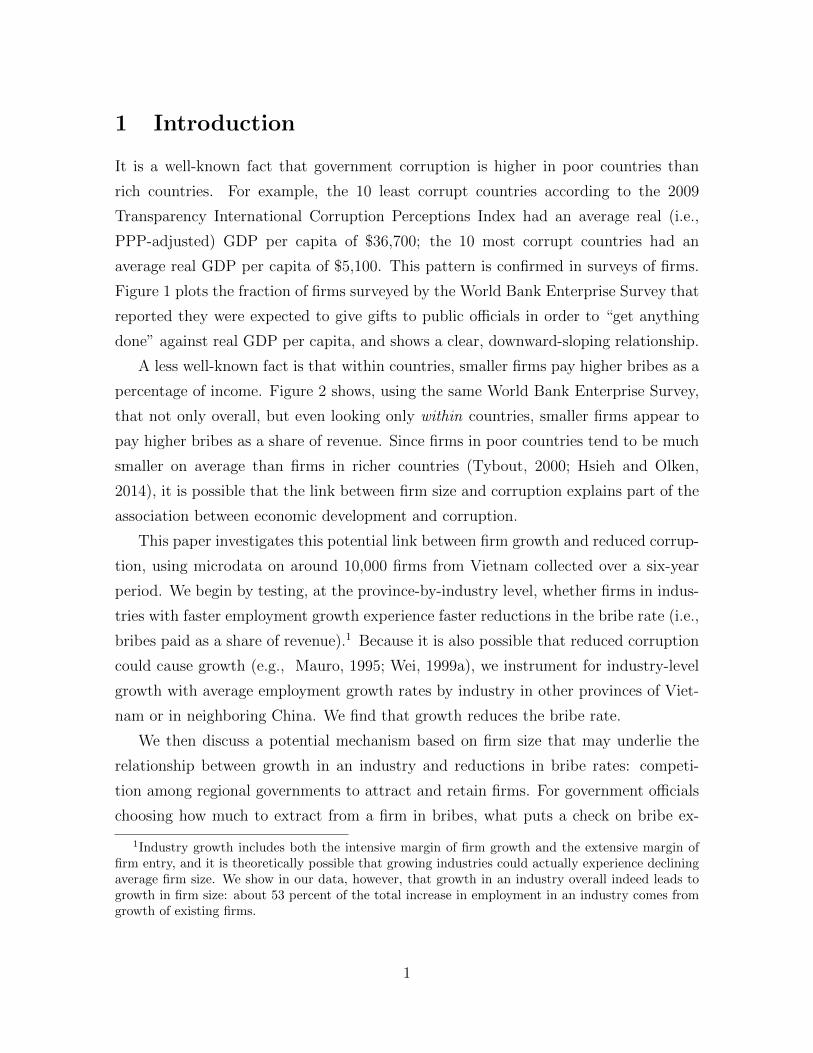
Figure 1 plots the fraction of firms surveyed by the World Bank Enterprise Survey that

reported they were expected to give gifts to public officials in order to “get anything

done” against real GDP per capita, and shows a clear, downward-sloping relationship.

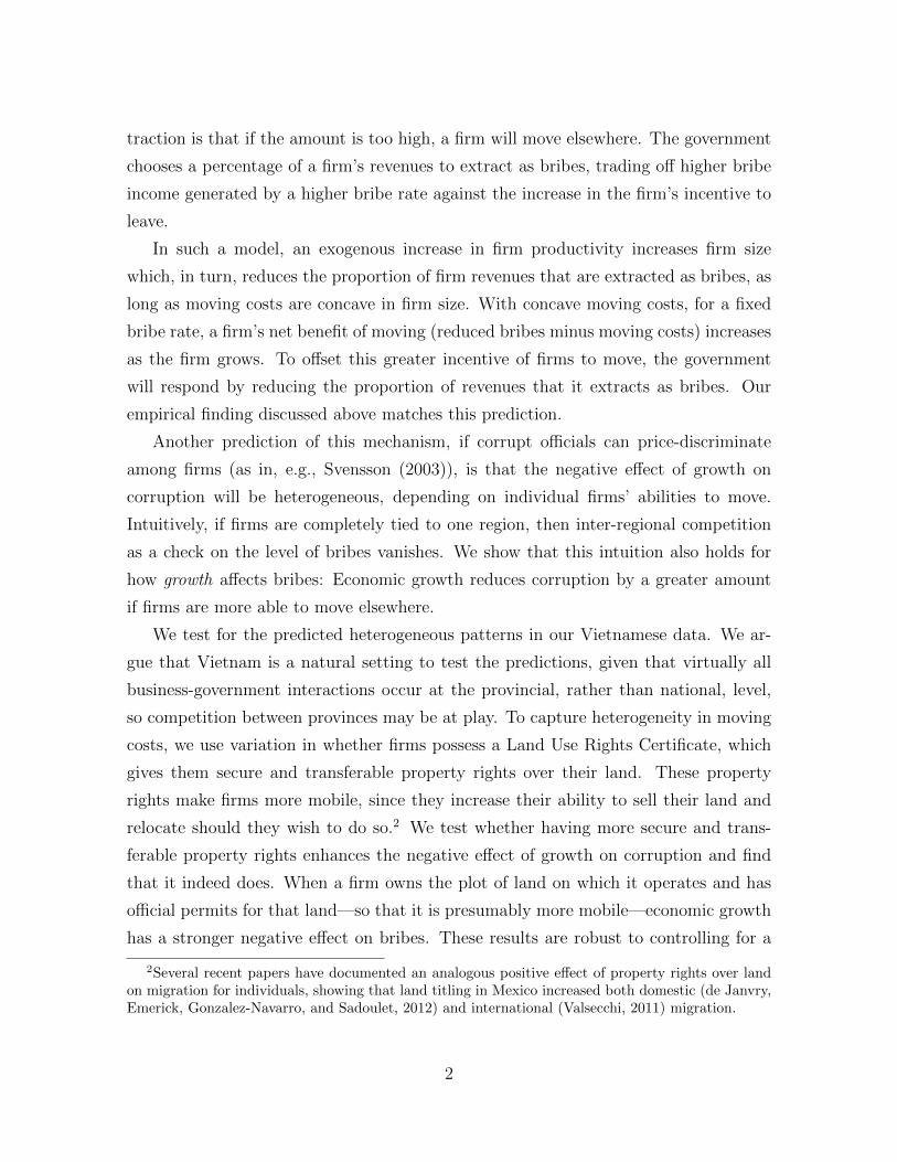
A less well-known fact is that within countries, smaller firms pay higher bribes as a

percentage of income. Figure 2 shows, using the same World Bank Enterprise Survey,

that not only overall, but even looking only within countries, smaller firms appear to

pay higher bribes as a share of revenue. Since firms in poor countries tend to be much

smaller on average than firms in richer countries (Tybout, 2000; Hsieh and Olken,

2014), it is possible that the link between firm size and corruption explains part of the

association between economic development and corruption.

This paper investigates this potential link between firm growth and reduced corrup-

tion, using microdata on around 10,000 firms from Vietnam collected over a six-year

period. We begin by testing, at the province-by-industry level, whether firms in indus-

tries with faster employment growth experience faster reductions in the bribe rate (i.e.,

bribes paid as a share of revenue).1 Because it is also possible that reduced corruption

could cause growth (e.g., Mauro, 1995; Wei, 1999a), we instrument for industry-level

growth with average employment growth rates by industry in other provinces of Viet-

nam or in neighboring China. We find that growth reduces the bribe rate.

We then discuss a potential mechanism based on firm size that may underlie the

relationship between growth in an industry and reductions in bribe rates: competi-

tion among regional governments to attract and retain firms. For government officials

choosing how much to extract from a firm in bribes, what puts a check on bribe ex-

1Industry growth includes both the intensive margin of firm growth and the extensive margin offirm entry, and it is theoretically possible that growing industries could actually experience decliningaverage firm size. We show in our data, however, that growth in an industry overall indeed leads togrowth in firm size: about 53 percent of the total increase in employment in an industry comes fromgrowth of existing firms.

1

traction is that if the amount is too high, a firm will move elsewhere. The government

chooses a percentage of a firm’s revenues to extract as bribes, trading off higher bribe

income generated by a higher bribe rate against the increase in the firm’s incentive to

leave.

In such a model, an exogenous increase in firm productivity increases firm size

which, in turn, reduces the proportion of firm revenues that are extracted as bribes, as

long as moving costs are concave in firm size. With concave moving costs, for a fixed

bribe rate, a firm’s net benefit of moving (reduced bribes minus moving costs) increases

as the firm grows. To offset this greater incentive of firms to move, the government

will respond by reducing the proportion of revenues that it extracts as bribes. Our

empirical finding discussed above matches this prediction.

Another prediction of this mechanism, if corrupt officials can price-discriminate

among firms (as in, e.g., Svensson (2003)), is that the negative effect of growth on

corruption will be heterogeneous, depending on individual firms’ abilities to move.

Intuitively, if firms are completely tied to one region, then inter-regional competition

as a check on the level of bribes vanishes. We show that this intuition also holds for

how growth affects bribes: Economic growth reduces corruption by a greater amount

if firms are more able to move elsewhere.

We test for the predicted heterogeneous patterns in our Vietnamese data. We ar-

gue that Vietnam is a natural setting to test the predictions, given that virtually all

business-government interactions occur at the provincial, rather than national, level,

so competition between provinces may be at play. To capture heterogeneity in moving

costs, we use variation in whether firms possess a Land Use Rights Certificate, which

gives them secure and transferable property rights over their land. These property

rights make firms more mobile, since they increase their ability to sell their land and

relocate should they wish to do so.2 We test whether having more secure and trans-

ferable property rights enhances the negative effect of growth on corruption and find

that it indeed does. When a firm owns the plot of land on which it operates and has

official permits for that land—so that it is presumably more mobile—economic growth

has a stronger negative effect on bribes. These results are robust to controlling for a

2Several recent papers have documented an analogous positive effect of property rights over landon migration for individuals, showing that land titling in Mexico increased both domestic (de Janvry,Emerick, Gonzalez-Navarro, and Sadoulet, 2012) and international (Valsecchi, 2011) migration.

2

propensity score that predicts having land use permits as a function of a variety of

other firm characteristics.

We also find similar patterns using a second measure of mobility: having operations

in multiple provinces. Firms with a presence in multiple provinces can more easily scale

back operations in one province and shift elsewhere where they might be subject to

less corruption. Thus, economic growth should put more downward pressure on bribes

for this group. We find empirical support for this prediction as well.

While the data are consistent with the inter-jurisdictional competition mechanism,

it is by no means the only potential mechanism for the negative effect of growth on

bribery. We discuss several alternative models, such as a fixed cost of anti-corruption

efforts or changes in industry concentration associated with the employment shock.

A key differentiating factor is that these other models do not generally explain the

fact that the responsiveness of bribes to shocks is stronger for firms that appear more

mobile. While no other model seems able to explain the complete set of facts we find

— so the mechanism we propose is likely at play — other mechanisms no doubt also

contribute to the overall effect of growth on bribery that we estimate empirically.

This paper builds on several strands of the literature. While many papers starting

with Mauro (1995) argue that corruption impedes growth, there is much less work

on the reverse direction, namely the idea that corruption may subside as countries

grow (notable exceptions include Treisman (2000) and Gundlach and Paldam (2009)).

This paper provides micro-evidence along these lines, along with suggestive evidence

of one potential channel. Our model of inter-jurisdictional competition builds on the

analysis of the problem of local governments setting tax rates (Epple and Zelenitz,

1981; Epple and Romer, 1991; Wilson, 1986), and in the corruption context, the idea

that competition can reduce bribe rates (Shleifer and Vishny, 1993; Burgess, Hansen,

Olken, Potapov, and Sieber, 2012). In particular, our model is most directly related

to the hypothesis advanced by Menes (2006), who noted in her qualitative study of

US cities that the ability of firms to relocate to other jurisdictions was one potential

reason why urban corruption in the pre-Progressive era was not more severe.

The remainder of the paper is organized as follows. Section 2 describes our data

and background information on Vietnam. Section 3 describes the empirical strategy,

and section 4 presents the results on the overall effect of growth on bribery. Section

5 discusses verbally how inter-jurisdictional competition could generate the pattern

3

documented in section 4 and further predicts that the growth-bribery effect varies with

a firm’s mobility. Section 6 empirically tests the additional prediction and discusses

alternative mechanisms through which growth could affect bribery. Section 7 concludes.

The formal theoretical model and robustness checks are available in an online appendix.

2 Setting and data

2.1 Background on Vietnam

Vietnam provides a unique opportunity to study the effect of firm growth on bribery

and how competition among subnational governments to attract firms affects bribery.

In 1986 Vietnam initiated the Doi Moi (Renovation) economic reforms, which elimi-

nated the role of central planning in the economy and opened its borders to interna-

tional capital and trade flows (Riedel and Turley, 1999). Since that time, the country

has achieved an average annual growth rate of 7 percent, ranking it among the very

fastest growing countries in the world over the period. Today, there are well over

350,000 private companies in Vietnam, operating in a range of sectors from food pro-

cessing and light manufacturing to sophisticated financial services.

The amount of corruption remains substantial in Vietnam. Most international

perceptions-based indices put Vietnam around the 30th percentile of corruption (where

lower is more corrupt). Similarly, Transparency International’s Global Corruption

Barometer reports that 44 percent of Vietnamese report paying a bribe in 2011 (Trans-

parency International, 2011).

Existing research has noted that corruption in Vietnam takes three main forms:

grease or speed money to fulfill basic tasks or services; the illegal privatization of state

property; and the selling of state power (Vasavakul, 2008). While all are undoubtedly

important, the first is the most directly observable and is the focus of our paper. The

key recipients are the traffic police, land cadres, customs officers, and tax authorities.”

These same offices were highlighted as the most corrupt in an internal study prepared by

the Party’s Internal Affairs Committee (Central Committee of Internal Affairs, 2005).

Gueorguiev and Malesky (2011) document that the same types of bribes are common for

firms, finding that 23 percent of businesses paid bribes to expedite business registration,

35 percent paid bribes when competing for government procurement contracts, and 70

4

percent paid bribes during customs procedures. Firms in Vietnam appear to accept

these payments as part of the cost of doing business (Rand and Tarp, 2012).

An important institutional feature of Vietnam is that corruption is largely subna-

tional. Via a series of laws in the early 1990s, most business-government interactions

were decentralized to the provincial level, including business registration, environmen-

tal and safety inspections, labor oversight, local government procurement, and land

allocation. Provincial departments of line ministries are “dual subordinate,” meaning

they report both to the provincial executive (the People’s Committee Chairman, or

PCOM), as well as the relevant national line ministry. In practice, however, appoint-

ments of department directors and budget allocations are set by the PCOM, closely

aligning department interests with those of the province. Moreover, proximity matters.

The PCOM interacts with department directors regularly, while the line ministries are

hundreds of kilometers away in Hanoi. As a result, many studies have documented

that the provincial government, more than the central government, is the relevant level

of government when thinking about the institutional climate facing firms, including

the degree of bribe extraction (Meyer and Nguyen, 2005; Tran, Grafton, and Kom-

pas, 2009; Malesky, 2008). Formal taxation is a notable exception; taxes on firms are

determined at the national, not provincial level.

Importantly, the powers of the provincial leadership over subordinate departments

and subprovincial governments (district and commune) also mean that corruption is rel-

atively centralized within individual provinces. The provincial leadership has the ability

to control the bribe schedule of the province both directly and indirectly. Provincial

leaders can punish corrupt subordinates with jail time or revoke their party member-

ship. They can also reduce the incentive for subordinates to bribe by changing their

own behavior, such as lowering their own cut of each activity, or not insisting on bribes

by subordinates for appointment to provincial government positions (which increases

the motivation and need for the subordinate to take money). More indirectly, they can

control the bribes extracted by subordinates through policy changes that reduce oppor-

tunities for bribes, such as reducing the number of required certificates and regulatory

inspections, formalizing specific waiting periods for documents, and increasing trans-

parency about the responsibilities of subordinate officials to businesses and citizens.

Indeed, one of the incentives to create the Provincial Competitiveness Index (PCI)

survey in the first place was to measure these differences in governance that affect

5

corruption and thereby motivate provincial leaders to reform their activities (Malesky,

2008, 2011).

As with all measures of governance in Vietnam, there is a high degree of subnational

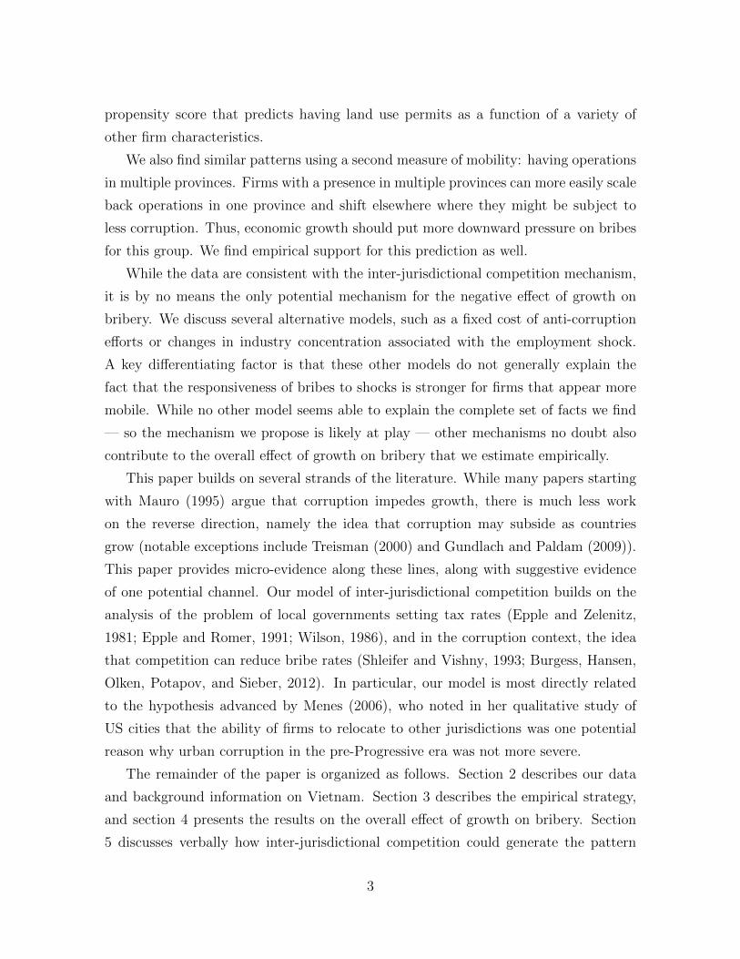
variation in firms’ responses about corruption in the data we use. Figure 3 shows

the distribution across provinces of the average response by firms for two corruption

questions from the PCI survey in 2011, the last year of our sample period. In the worst-

scoring province, 79 percent of private firms reported that firms in their line of business

were subject to bribe requests. In the best-scoring province, a substantially smaller 21

percent claimed such activities were common. Similarly, high inter-provincial variation

is observed for the share of revenue paid in bribes by firms, the main dependent variable

in our analysis. In 2010, 37.5 percent of firms in the most corrupt province said bribe

payments exceeded 2 percent of their annual revenue, compared to 5.5 percent in the

lowest province.

2.2 Description of data

To examine the effect of growth on corruption, we use two firm-level data sets, the

Vietnam PCI Survey (Malesky, 2011), and the annual enterprise survey collected by

the General Statistics Office (GSO) of Vietnam, henceforth referred to as the PCI

and GSO data, respectively. For each data set, we have five years of repeated cross-

sectional firm-level data from 2006 to 2010. We also use aggregate employment data

at the industry-year for 2006 to 2010 from the Chinese Yearbook of Labor Statistics.3

The PCI survey is a comprehensive governance survey of formal sector firms across

Vietnam’s 63 provinces. The PCI (as well as the GSO) regard formal firms as those

with an official registration certificate from their provincial Department of Planning

and Investment, thereby excluding household operations without such documentation.

The PCI survey team randomly sampled from a list of at least partly private companies

with a tax code provided by the province’s tax authority. Stratification was based on

firm size, age, and broad sector (agriculture, services, construction and industry) in

order to accurately reflect the population of firms in each province. The PCI survey

3The PCI survey is conducted in the early part of each calendar year (March-June). Informationabout firms’ business and operations refer to the previous calendar year. For variables regarding bribepayment, it is reasonable to think that firms are also reporting based on the past year. We thereforelag the PCI survey by one year before merging with the GSO or Chinese Yearbook data. The 2006to 2010 timeframe thus corresponds to the PCI surveys conducted in early 2007 through early 2011.

6

contains basic firm-level information, including the firm’s ISIC 2 digit industry code,

location (province), year of establishment, total assets, and total employment.

What makes the PCI survey well-suited for our study is that it has a module on

corruption and red tape faced by the firm. The most relevant question that matches

our theoretical predictions is the amount of unofficial payments to public officials the

firm makes, expressed as a percentage of its revenue. To the best of our knowledge, this

data set is the only frequently repeated cross-section of firms’ corruption experiences

that is representative at the sub-national level in the developing world.

For our analysis, we merge the PCI firms with aggregate employment information

constructed from the GSO survey at the industry-province-year level.4 For industry, we

use the ISIC alphabetical category. The GSO data also include all formal sector firms in

Vietnam, both private and state-owned. We restrict our sample to private firms in order

to match the PCI sample. The sampling strategy for small size firms (firms with fewer

than 10 employees) for the GSO survey varies from year to year. Therefore, to ensure

that we have a consistent and well-defined measure for a province-industry’s economic

conditions in a given year, we exclude the small firms with fewer than 10 employees

when constructing the industry-province-year employment and before merging with

the PCI. Panel A of Table 1 presents summary statistics for all the merged firms in

the PCI data. For our main analysis, we restrict the PCI sample to firms with 10 or

more employees reported for the previous year in order to match the GSO sample. We

used lagged employment since it is determined prior to our bribe measure.5 Our final

analysis data set contains 10,901 firms that meet this sample inclusion criterion. Panel

B of Table 1 reports the summary statistics for the final analysis sample. Results on

the full sample of firms are presented in Appendix A.

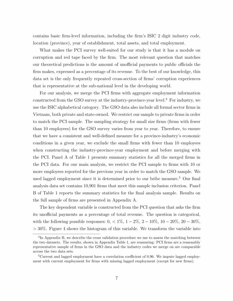
The key dependent variable is constructed from the PCI question that asks the firm

its unofficial payments as a percentage of total revenue. The question is categorical,

with the following possible responses: 0, < 1%, 1− 2%, 2− 10%, 10− 20%, 20− 30%,

> 30%. Figure 4 shows the histogram of this variable. We transform the variable into

4In Appendix B, we describe the cross validation procedure we use to assess the matching betweenthe two datasets. The results, shown in Appendix Table 1, are reassuring: PCI firms are a reasonablyrepresentative sample of firms in the GSO data and the industry codes we merge on are comparableacross the two data sets.

5Current and lagged employment have a correlation coefficient of 0.96. We impute lagged employ-ment with current employment for firms with missing lagged employment (except for new firms).

7

a scalar by assigning each response the middle of the corresponding bin, using 0.5%

for the < 1% category and 35% for the > 30% category. The mean of this variable

is 3.4%. While this may seem small, recall that this is a percent of revenues, not

profits. If firms averaged 10% net profit margins, for example, this would be the same

magnitude as a 34% profit tax. (In the empirical section below, we also consider an

alternative specification using ordered probit models that allows the model to determine

appropriate breakpoints; results are similar).

The PCI requires general managers or owners to complete and mail in the survey,

although there is no way to formally guarantee that the task was not delegated to a

subordinate. Over 65 percent of respondents list their position as CEO, Director, or

Owner, suggesting that the respondents would generally be in a position to know about

bribe-payments, and that delegation is not a major threat to our analysis.

The median firm in our final sample has been in business for four years and has

between 10 and 49 employees, which is nearly identical to the GSO census aggregates.6

Figure 5 shows the relationship between the bribe rate and firm size in our sample.

Larger firms appear to be paying a smaller percentage of their revenues in bribes.

(Larger firms might still pay a larger amount per firm in bribes, but the relevant

metric for gauging the size of the distortion – and the prediction in the theoretical

model discussed below – is the bribe rate.)

In addition to corruption activities, the PCI also has variables related to the firm’s

property rights status that we use to measure the firm’s mobility, such as whether the

firm owns the land that it occupies and whether the firm has a Land Use Rights Cer-

tificate. We will describe these variables in more detail when we discuss the empirical

results. The second proxy for mobility we have in the data is whether the firm operates

in multiple provinces. While the majority of firms are wholly located in one province,

multi-province firms are reasonably common, with 31.4 percent having operations in

provinces besides their main location.

Table 1 also summarizes several control variables we use, including the proportion

of registration documents the firm has (a proxy for a firm’s general propensity to

complete formal paperwork), whether the firm was formerly a household firm, whether

6We use the GSO fine-grained data on employment to impute the mean and median employmentlevel within the PCI ranges. The median size of firms in the GSO that are between 10 and 49 employeesis 19 employees.

8

it is a former state-owned enterprise, whether the owner is a government official, and

whether the government has an ownership stake in the firm.

Our empirical strategy uses aggregate shocks to a firm’s industry size in other

provinces of Vietnam, or in China, to predict firm growth in a given province and

industry. In the final merged data set, we have 18 distinct industry categories (see

Appendix Table 2 for a description of the industries). The main GSO variable we use

in the analysis is the log of aggregate employment in the industry-province-year, which

is also summarized in Table 1.

To construct our China-based instruments, we use the China Labor Statistical Year-

book to calculate industry-year specific total employment in China. The Yearbooks re-

port the number of employed persons by industry, including employment in state-owned

enterprises (SOEs), collectives, foreign joint ventures, and private firms/individual

workers in urban areas. Note that industry-level employment data is not available

for rural areas during this period. Industry codes are based on the Chinese GuoBiao

(national code) system, and are broadly consistent with the broad alphabetical code

in ISIC Revision 4.

3 Empirical strategy

The hypothesis we aim to test is that firm growth has a negative effect on bribes, or

more specifically, bribes as a percentage of the firm’s revenues (Bribes). Suppose we

had a measure of firm productivity Aipjt for firm i in industry i in a particular province,

p, and time, t. One could in principle test the hypothesis via OLS as follows:

Bribesipjt = α + βAipjt + εipjt (1)

The dependent variable is the amount that firm i paid in bribes as a percentage of

its revenue in year t. The prediction is that β in Equation (1) is negative, so that on

average productivity growth reduces bribes.

There are two issues with estimating Equation (1) directly. The first is a data

problem: we do not directly observe TFP or output prices in the data, so, empirically,

we use total employment in the province-industry-time cell (Employpjt) as a proxy.7

7The reason we cannot calculate TFP directly is that we do not have reliable measures of revenue,

9

Under the assumption that factor prices are constant, changes in employment reflect

changes in A (this is true, for example, in the model we present in Appendix C), so

to the extent we can find a measure of employment that is exogenous with respect to

the bribe rate b, we can replace A with Employ and test the same predictions. The

exogenous variation in Employ available in our setting is at the industry-province-year

level, rather than the firm level.

Our independent variable is aggregate employment growth in a given industry-

province-year cell, rather than firm size. Whether aggregate growth is driven by growth

in firm size is an empirical matter; changes in Employpjt could be driven by entry, or

by growth in existing firms, or some combination. For our IV strategy using Chinese

data (described below), only aggregate employment data are available, so we are not

able to calculate average firm size. However, we can decompose aggregate growth with

the Vietnam firm-level data, and we find that there is correlated growth along both

margins: Predicted total employment is highly correlated with both average firm size

in the GSO data and the number of firms. Specifically, if we regress log mean employ-

ment and log total number of firms in province-industry-year group on employment in

the rest of Vietnam log(Employp−jt), controlling for province-industry and year fixed

effects (which is the setup for our first IV strategy described below), the coefficients

are 0.341 and 0.301 respectively; both are significant at the 1 percent level. Mathe-

matically, the sum of the two coefficients is equal to the coefficient when regressing

the endogenous variable, log total employment in the province-industry-year group, on

log(Employp−jt). Hence, the ratio of each of the two coefficients to their sum tells us

how much a shock to log(Employp−jt) affects the intensive versus extensive margin. In

our setting, about 53 percent of employment growth (=0.341/0.642) is on the intensive

margin. An important point to keep in mind is that, while our theoretical predictions

and interpretation of the empirical results focus on the intensive margin, i.e. firm

growth, our empirical results are not able to distinguish between these two margins.

Once we have Employ as a proxy for industry-level productivity growth, a second

issue remains which is that employment levels are potentially endogenous to the bribe

level b. Thus, we estimate Equation (1) via two IV strategies, as described below.

capital stock, and wages in our data.

10

3.1 Rest-of-Vietnam IV

The first instrumental variable strategy we use is employment in the firm’s industry

in Vietnamese provinces other than its own, controlling for common national year

fixed effects and province-by-industry fixed effects. The IV strategy is predicated

on industry-specific employment (or TFP) shocks in an industry being similar across

provinces (i.e., on there being a strong first stage). For example, for an industry that

supplies to the world market, an increase in output prices would correspond to an

increase in Aijt.

A key identification assumption is that industry-specific bribe-setting is determined

independently by each province. In particular, we are ruling out a large-scale national

crackdown on corruption specific to an industry in a given year, which would violate

this assumption (note that a national crackdown across all industries would be absorbed

by year effects and would not be a problem for our identification strategy; likewise,

different average levels of corruption in different regions or industries would be absorbed

in region-by-industry fixed effects and would not be a problem). The assumption

matches the institutional context of corruption in Vietnam as discussed in Section 2.1

in which corruption is largely a provincial matter.

Our first stage specification using the leave-one-out Vietnam IV is as follows:

log(Employpjt) = α + β log(Employp−jt) + νpj + µt + εpjt. (2)

The outcome variable, log(Employpjt), is log total employment for industry j in year

t in province p. The variable log(Employp−jt) is log total employment for firms in

industry j and year t in all provinces other than p. We control for province-industry

(pj) and year (t) fixed effects, so the specification is capturing differential changes in

employment across industries over time, netting out common national time trends and

different average levels by province-industry cell.

The corresponding second stage equation is:

Bribesipjt = α′ + β′ ̂log(Employpjt) + ν ′pj + µ′t + ε′ipjt. (3)

The IV varies at the industry-province-year level but we implement two-way clustering

at the province and industry-year level to correct for possibly correlated errors across

11

time and industry and because most of the variation in the IV (and all of the variation

in the case of our China IV) is at the industry-year level.

3.2 China IV

One concern with the rest-of-Vietnam IV is that it could be correlated with common

industry-year specific shocks that affect both firm growth and bribe payments, such as

a time-specific national regulatory change or a national industry-specific crackdown on

corruption. These could be either for exogenous reasons, or potentially an endogenous

response of one province to another (as in the model we present in Appendix C), in

which firms best-respond to one another’s bribe policy). Thus, we also implement a

second identification strategy using growth rates from outside of Vietnam that is not

as subject to these concerns.

For our second IV strategy, instead of instrumenting for Vietnamese employment

in a particular industry in a particular province with employment in other provinces

of Vietnam, we instrument using employment in China. The idea is that many indus-

tries in Vietnam and China are subject to the same global business cycles and price

and technology shocks, and hence industry-level growth is correlated across the two

countries. But, because China is so much larger than Vietnam, it is unlikely that there

would be reverse causation where changes in a particular industry’s corruption level in

Vietnam would substantially affect employment growth in China.

Specifically, we estimate the following first-stage regression:

log(Employpjt) = α + β log(EmployChinajt) + νpj + µt + εpjt, (4)

where we again include province-industry and year fixed effects and cluster at the

province and industry-year level.

3.3 Multiple IVs

The first stage equations described above constrain the effect of a shock to A or Employ

in the rest of Vietnam to be the same across industries, and, similarly, the effect of a

shock to an industry in China on Vietnamese firms to be the same across industries. In

principle, some industries can have positively correlated growth rates between provinces

12

in Vietnam or between China and Vietnam (say, due to common worldwide demand

shocks), and some industries can have negatively correlated growth rates (say, because

provinces or the two countries compete for a fixed amount of global business). Thus,

we also allow the first stage coefficients to vary by industry. The first stage allowing

for different β’s for each industry j is as follows for the China case:

log(Employpjt) = α + βj log(EmployChinajt) + νpj + µt + εpjt. (5)

Allowing the first stage coefficient to vary by industry is equivalent to having one

instrument per industry, e.g., log(EmployChinajt) interacted with an industry dummy.

The multiple-IV specification for the rest-of-Vietnam approach is analogous.

In practice, for the rest-of-Vietnam IV strategy, the constraint of a uniform β across

industries is reasonable, and the single IV has more precision. For China, the multiple

IV first stage fits the data better and yields more precise results.

In the next section, we present our results on the effect of growth on bribery, using

both the rest of Vietnam and China approaches, and using both a single and multiple

instruments.

4 Results

This section presents evidence that a positive shock to aggregate productivity decreases

unofficial payments by firms.

4.1 First stage results

To estimate the first stage regressions, we use the GSO data and compute total em-

ployment for each pjt (province-industry-year) cell. For the within-Vietnam IV, the

instrument also uses the GSO data and is aggregated at the p−jt level. For the China

IV, the Chinese Yearbook is used and the data vary at the jt level. For industries, we

classify firms into their alphabetical ISIC code (18 industries in total).8 Each observa-

tion in the first-stage regressions we present is a pjt combination.

8We have an equally strong first stage using the finer two-digit ISIC codes, but the broader alpha-betical codes are more robust to differences in classification across the GSO and PCI data sets, andfor the Chinese data, the data are aggregated at the coarser level.

13

We report the first stage results from estimating Equations (2) and (4) in Table

2. We report standard errors with two-way clustering at the province and industry-

year level throughout. As seen in column 1, the first stage coefficient is positive and

significant at the 1 percent level using the within-Vietnam IV; the F-statistic is 26.9.

The coefficient on log(Employp−jt) is 0.642. This means that for a 10 percent increase

in total employment in other provinces for industry j in year t, there is a 6.42 percent

increase in one’s own province. Theoretically, if the aggregate shock propagates to all

regions equally, we should observe a coefficient of 1; the coefficient of 0.642 suggests

that much but not all of the temporal variation in productivity in Vietnam is aggregate

to an industry.

Column 2 shows the first stage for the China IV. The first stage coefficient is

remarkably similar at 0.622. The coefficient is significant at the 5 percent level, but the

standard error is substantially larger than for the Vietnam IV, which is not surprising

because provinces in Vietnam might be more likely to supply the same markets and

thus respond to the same demand shocks, merging between data sets is more prone to

error with the China approach because the Chinese industry codes differ slightly from

the Vietnamese ones, and the composition of firms in the Chinese data is somewhat

different (e.g., it comprises only urban firms). The F-statistic is 3.89. Because of this

low (for an instrument) F-statistic, we focus more on the multiple-IV variant when

using the China IV strategy, because it has a stronger first stage.

The multiple-IV first stages for both Vietnam and China are reported in Appendix

Table 3.9 The F-statistics for the set of instruments are 7.99 using Vietnam and 8.37

using China. For Vietnam, the single IV gives a stronger first stage, while with China,

the multiple-IV approach gives a stronger first stage. We report the results for all four

permutations, which yield similar second-stage results, but in the discussion, we focus

mostly on the single-IV Vietnam results and multiple-IV China results.

9The positive first-stage coefficients for transportation and storage, information and communica-tion, financial and insurance activities, real estate, professional and scientific activities, education,health, and administration could reflect global business cycles, common interest rate shocks, and syn-chronicity in public service provision. The negative first-stage coefficient for mining and quarrying issurprising but could result from inter-regional competition for global demand, which outweighs theeffect of common global market shocks.

14

4.2 Effect of employment growth on bribes

The IV results are shown in Table 3. The top panel presents the within-Vietnam

instrument and the bottom panel, the China instrument. All specifications control

for province-industry and year fixed effects, and standard errors are clustered at the

province and industry-year levels.

Starting with the top panel, column 1 uses the single instrument and has a coeffi-

cient of -1.704, which is significant at the 5 percent level. Growth in firm employment

leads to a drop in the rate of bribe extraction from firms. The coefficient magnitude

suggests that a 10 percent increase in a firm’s employment level leads to a 0.18 per-

centage point decline in the bribe rate. Column 2 uses multiple IVs (one per industry)

and finds a similar result.

Panel A, columns 3 and 4 report the reduced form results. Our outcome variable,

which measures the degree of corruption firms face, is the unofficial payments as a per-

centage of revenue. As discussed above, it is a categorical variable, which we linearize

by using the middle of each category. We estimate two versions of the reduced form

estimate, one using the linearized variable and one using an ordered probit specifica-

tion that allows the regression to determine the precise cardinalization of each of the

categories. The results in column 3 show that the coefficient for log(Employp−jt) is

-1.203, and significant at the 5 percent level. Column 4 reports the results from an

ordered probit specification. The coefficient is again negative and significant at the 5

percent level. The ordered probit results suggest that the negative relationship shown

is not merely driven by the linear functional form.

To interpret magnitudes, note that column 1 implies that a doubling of total em-

ployment in the industry is associated with a 1.2 percentage point reduction in informal

payments, or about 35 percent of the mean level. Translated into an elasticity, this

suggests an elasticity of the informal payment rate (i.e., the share of revenues devoted

to informal payments) with respect to predicted firm size of about -0.5. Since this

elasticity is substantially less than 1 in absolute value, it implies that while the share

of firm revenues paid in bribes declines as A increases, total unofficial payments, which

is the bribe rate multiplied by revenues, increase. While the bribe rate is the key

parameter that determines aggregate distortions due to corruption, it is worth noting

that given this elasticity, the amount of corruption in absolute dollar terms actually

15

increases even though the rate does not.

The fact the estimates imply that bribes as a percent of revenue fall, but that the

total magnitude of bribes rises, suggests that bribes are indeed responding to changes

in firm size – we can reject both the null that bribes are constant in levels (i.e. each

firm pays a fixed bribe regardless of size), and also the null that bribes as a percent

of revenue are constant or reported to be constant (i.e. bribes as a share of revenue is

falling). The fact that bribes as a share of revenue falls, but the absolute level of bribes

rises, is consistent with the theoretical model presented in Appendix C and discussed

briefly in section 5.

The results in Panel B using the China instrument are similar to the those in Panel

A, though as discussed above, the single-instrument version of the Chinese IV version

is less precisely estimated. The single-IV estimate, reported in column 1, is -1.509,

similar in magnitude to the within-Vietnam analogue, though the coefficient is not

statistically significant. Column 2 of Panel B uses multiple IVs, and the coefficient is

-1.149 and significant at the 5 percent level. Both the point estimate and precision are

remarkably similar across the Vietnam and China specifications.

The point estimate for China of -1.149 in column 2 implies that a 10 percent increase

in employment leads to -0.115 percentage point decline in bribe rate, or a doubling of

employment leads to 0.8 percentage point decrease in the bribe rate, which is 23.5

percent of the mean level. The implied elasticity of the informal payment rate with

respect to predicted firm size is -0.34, similar though slightly smaller than the elasticity

of -0.5 we estimate using the single within-Vietnam IV. The reduced form OLS and

ordered probit results reported in column 3 and 4 are negative but insignificant.

To recap, across our different IV specifications—using industry employment else-

where in Vietnam, or alternatively industry employment in China as predictors of firm

size—we find that growth has a negative effect on the degree of government officials’

bribe extraction from firms.

5 Inter-jurisdictional competition as a mechanism

One mechanism that could generate the finding in the previous section is competition

among jurisdictions to retain or attract firms. Consider a model in which governments

choose how much to extract from firms to maximize their bribe revenue. We develop

16

and solve such a model, and it generates the prediction that bribes as a fraction of

revenues decrease with firm growth under reasonable assumptions. This model is not

the only explanation for the empirical fact presented in the previous section, but is one

possible explanation. Moreover, the model has other testable predictions which we will

investigate empirically in the next section.

The full model is available in Appendix C, but here we describe the intuition and

results in a bit more detail. The government in each province sets a bribe rate, which is

the percent of a firm’s revenues that it must pay in bribes. Next, firms in each province

choose whether to stay in the province or relocate to the other province. Finally, firms

choose their factors of production, they produce, and the government collects bribes.

The firm will choose to stay in its current province if and only if profits there are

greater than its profits in a new province, less moving costs. One can consider shocks

to productivity that generate firm growth. With a positive shock to firm productivity

and hence firm size, if moving costs scale up less than one-for-one with firm size, then

firm growth will lead to a decrease in the equilibrium bribe rate (Prediction 1). When a

firm grows, a given bribe rate imposes a larger cost on the firm, making it more prone

to leave for a lower-corruption locale. This force drives down the equilibrium bribe

rate due to inter-regional competition. However, at the same time, the cost of moving

rises as firms expand in size to take advantage of the higher productivity. This instead

drives up the equilibrium bribe rate. If moving costs do not scale up too steeply, then

the first effect dominates and growth decreases the bribe rate.

In practice, there are likely some fixed costs of moving, so it seems reasonable that

total moving costs are indeed concave in firm size. Prediction 1 then matches the key

result of the paper shown in the previous section.

It is worth noting that another prediction is that the total amount of bribes ex-

tracted from the firm will increase with a positive productivity shock. To see this, note

that the firm’s moving decision is a tradeoff between its total moving costs and its total

bribes. When a firm grows, the firm’s moving costs increase, and thus the government

can retain the same firms even with a higher total bribe extraction. This prediction

also holds in the data, as discussed in the previous section.

Next, we consider how the effect of a productivity shock on bribes varies across

firms with different observable-to-the-bureaucrat moving costs. We will focus on the

firm’s property right status or multi-province operations as determinants of its moving

17

costs in the empirical analysis in the next section. The model prediction is that the

bribe rate falls more after a positive shock to productivity for firms with low observable

moving costs (Prediction 2). The intuition is that the fraction of such firms who are on

the margin of moving is larger, so a given change in bribes will induce a larger number

of them to leave.

Before turning to the empirical test of Prediction 2, it is worth noting the analogy

between bribes and taxes. For firms, a bribe is an additional payment to government,

analogous to a tax. Our model is therefore similar to models of inter-regional tax com-

petition. The key distinction of our results compared to the previous literature is that

we focus not just on the equilibrium level of taxes/bribes, but also examine how the

level of bribes changes with productivity shocks. It is this comparative static that gen-

erates predictions about how growth affects the amount of corruption in the economy.

Our result on how the relationship between productivity shocks and the equilibrium

bribe rate varies based on the firm’s ease of relocating to another jurisdiction is also

novel in the literature, to the best of our knowledge.

Also worth noting is that to the extent that taxes follow similar patterns to bribes,

another implication of the model is that taxes on firms should also be lower in rich

countries than in poor countries. There is suggestive evidence along these lines: Gor-

don and Li (2009) show that for poor countries (with per-capita GDP below $745),

corporate income taxes represent 7.5 percent of GDP, whereas for rich countries (with

per-capita GDP above $9,200), corporate income taxes represent only 4.5 percent of

GDP, although they suggest a different explanation than the one proposed here.

Finally, we discuss the exclusion restriction of our two instrumental variable strate-

gies in light of the model. Results 1 and 2 consider the effect of a common shock

to all jurisdictions (provinces). To the extent that the rest-of-Vietnam employment

(summed across all other regions) reflects the common component, it is a valid instru-

ment for testing the effect of an aggregate shock (i.e., the two predictions of the model).

However, the rest-of-Vietnam instrument could also reflect shocks idiosyncratic to all

other provinces, but not a province itself. One could imagine that shocks to other

provinces can affect the bribe setting in a province (if that information is public), with

officials reacting to the changed desirability of other provinces. This is particularly so

for shocks to places where firms are likely to move to. Conversely, a shock to bribes

in one province could affect employment in other provinces through firm relocation.

18

Either of these channels would be a problem for the excludability of employment in

other provinces as an instrument for employment in province i in equation (3).

To address this concern, we perform an additional robustness check by construct-

ing the rest-of-Vietnam IV using total employment in the same industry in other re-

gions instead of other provinces. To the extent that firms are more likely to move

within their own region, this additional analysis helps to alleviate the concern of the

above-mentioned bribe setting responses which would violate the exclusion restriction–

provincial governments are less likely to respond to idiosyncratic shocks in other regions

since incumbent firms are less likely move there; therefore the alternative instrumental

variable strategy seeks to capture the effect of aggregate industry-year shocks which

affect the equilibrium bribe rate as in our model. The result shown in Appendix Table

7 is qualitatively similar to Table 3.10 Moreover, as long as firms are less mobile across

national boundaries, which seems highly plausible, the China instrumental variable

strategy also helps to address these concerns.

6 Heterogeneous effects by firms’ moving costs

We presented evidence in section 4 that economic growth (specifically, an increase in

firm employment) reduces the rate of bribe extraction. The inter-jurisdictional com-

petition idea described in the previous section generates this prediction, but is not the

only explanation for why an increase in employment reduces bribes. For example, it is

possible that bureaucrats simply have diminishing marginal utility of income relative

to the risk of being caught and going to jail, so that as it becomes easier to extract

revenues, they reduce rates. However, a key prediction of inter-jurisdictional competi-

tion, as opposed to potential alternative explanations, is that the effect of an increase

in firm productivity on the bribe rate should be greater in magnitude when firms are

more mobile. 11

10We also investigated the extent to which these results would still hold even with mild violations ofthe exclusion restriction, using the ‘plausibly exogenous’ methodology of Conley, Hansen, and Rossi(2012), in which they allow the instrument Z to affect the outcome directly through the equationY = Xβ+Zγ+ ε for a range of γ values. The results are reported in Appendix Table 8. We find thatthe IV estimates of the effect of firm growth on bribes remain negative even if we allow for reasonablysized violations of the exclusion restriction (i.e. up to γ as large as β.)

11The idea that firms that are less mobile are treated differently by local officials in Vietnam isconsistent with Rand and Tarp (2012), who show using different data that firms that appear less

19

We test that prediction with the following estimating equation:

Bribesipjt = α+βAipjt+γAipjt×MovingCostipjt+δMovingCostipjt+νpj+µt+εipjt (6)

The prediction is that γ in Equation (6) is positive, so that the reduction in bribes

as firm growth increases is smaller for firms with higher moving costs. Again, we

estimate the equation using both of our IV strategies.

As measures of MovingCost, we use two firm characteristics. First, we use variation

across firms in their property rights over the land they operate on, and, second, we use

variation in whether the firm is based in one province or multiple provinces.

Property rights

In Vietnam, firms can have three types of tenure over the land on which they operate:

renting, owning the land with official land use rights, and owning the land without offi-

cial land use rights.12 Specifically, for firms that have purchased their land, they may

or may not have a land use rights certificate (LURC). Firms, intending to strengthen

their property rights, submit the LURC application and related documents, such as

map of the area and business plan, to the provincial Land Use Right Registration Of-

fice. Conditional on having purchased land, having an LURC makes it easier for the

firm to move, because the firm can sell or trade its certificate if it decides to relocate to

another province, whereas land without an LURC can easily be expropriated by local

authorities (Kim, 2004; Do and Iyer, 2003), making it harder to sell.

It is not ex ante obvious whether firms that rent face higher or lower relocation costs

than those that own. For example, renters cannot recoup the value of any improvements

they made to the property and may be locked into hard-to-renegotiate long-term leases,

but they do not face transaction costs from having to sell property. What is clear

though is that conditional on owning, transaction costs are lower for those with an

LURC. We therefore examine heterogeneity across these different levels of moving

costs: firms that rent land versus purchase land, and conditional on having purchased

land, firms that have LURCs versus those that do not.

mobile pay higher bribes.12Note that while we use the term “own,” the more precise term would be “purchased” since in

Vietnam, firms can purchase land, but in a technical sense, the state still owns all of the land.

20

We estimate a model that interacts log(Employpjt) with these measures of prop-

erty rights. In general, since we have a repeated cross-section of firms, not a panel,

there is a potential endogeneity problem if we use θ at the firm level (e.g., firms could

adjust their θ in response to a shock in A). For the LURC variable, we know the year

the firm acquired the certificate, so we can also use lagged values of LURC owner-

ship to address this concern.13 In addition to interacting these measures of movings

costs with log(Employpjt), we also show the results controlling for the interaction of

log(Employpjt) with average firm size in the industry to isolate the effects of land own-

ership status from other general industry characteristics, in case land ownership and

LURC status are correlated with firm size. We also examine a host of other controls

below, all interacted with log(Employpjt), to capture the fact that having an LURC is

not randomly assigned (e.g. LURC firms may be more willing to pay bribes to obtain

permits, are older, etc).

The first two columns of Table 4 use a single IV and compare firms that own land

and have an LURC against the omitted category of all other firms, both those that

are renting and those that own land without an LURC. In Panel A, the coefficient

on the interaction with log(Employpjt) in column 1 is -0.292 and significant at the 5

percent level, suggesting that indeed firms with LURCs have the largest reduction in

bribe rates as predicted employment increases.

To interpret the magnitudes, recall that the average effect of increasing employment

on reduced corruption from Table 3 is -1.704. The results in column 1 suggest that

the impact is about 17 (=0.292/1.704) percent larger in magnitude for firms with an

LURC than those without one.

As shown in column 2, the coefficient on the LURC interaction is insensitive to

whether we control for industry average firm size interacted with log(Employpjt)14,

suggesting that the land ownership and LURC variables are really picking up something

about the firm’s property rights rather than industries with larger or smaller firms.

Columns 3 and 4 also include the interaction between the firm owning land and

log(Employpjt). The coefficient on the interaction of the firm owning land and hav-

13Unfortunately, we do not know the year the firm purchased its land, so we cannot do the analogousexercise for land ownership. In Appendix Table 9, we show the results using contemporaneous LURC.

14The industry average firm size is computed as the average employment (with the categoricalvariable recoded using the GSO data to calculate the within-category mean, as detailed in AppendixD) among PCI firms in the same industry pooled over all years.

21

ing an LURC and log(Employpjt) is now the additional impact of owning an LURC

conditional on owning land, i.e., comparing firms that own land and have an LURC

with those that own land and do not have an LURC. The LURC interaction term in

this specification is the most direct test of the theoretical prediction. The interaction

coefficient of -0.12 is negative (column 4), consistent with the prediction, but quite

noisily estimated.15

Columns 5 to 8 repeat columns 1 to 4, but using multiple IVs for Vietnam, and

the estimates are broadly similar. Panel B then presents the results using the Chinese

IV. It is reassuring that the results are similar using different IV strategies and are

robust to controlling for firm size. Nonetheless, possessing an LURC is not randomly

assigned, and could be correlated with other firm characteristics. Possessing an LURC

is indeed correlated with a variety of other firm characteristics (Appendix Table 11),

but, reassuringly, the findings are robust to controlling one-by-one for the interaction of

these possible correlates of property rights with log(Employpjt), as well as controlling

for the interaction of propensity scores for having an LURC and owning land with

log(Employpjt) (Appendix Tables 12 and 13).

Firms operating in multiple provinces

The PCI data provide a second proxy for firm mobility that we can use to test for

heterogeneous effects: having operations in multiple provinces. Of the firms in the

sample, 31.4 percent have operations in at least two provinces. These firms with some

of their operations elsewhere likely have a more credible threat to wholly move to

another province or simply focus their expansion plans elsewhere, making them more

observably mobile to provincial officials. Of course, these may be different on other

dimensions as well, but this nevertheless provides another way of testing the idea that

bribes are more elastic with respect to firm size for these plausibly more mobile firms.

Table 5 examines heterogeneity based on multi-province operations. The proxy

for MovingCost is dummy for operating in at least one other province besides the

province where the firm is headquartered. The interaction coefficients are both -0.26 in

columns 1 and 2 (significant at the 1 percent level). The main effect of log(Employpjt)

in column 1 is -1.704, so the interaction coefficient implies that having multi-province

15We have also estimated ordered probit reduced form specifications with broadly similar results;see Appendix Table 10.

22

operations increases the negative effect of growth on the bribe rate by 15 percent.

We find similar results, reported in Panel B, using the Chinese IV. Focusing on the

multiple-IV results in column 3 and 4, the effect of growth on bribery is stronger for

mobile firms, with the result significant at the 1 percent level.

Appendix Tables 14 and 15 present the battery of robustness checks. For the

preferred specifications of the single-IV Vietnam approach and the multiple-IV China

approach, the results are essentially similar.

To summarize our main empirical results, first, we showed in section 4 that positive

productivity shocks for firms reduce corruption. Second, in this section we presented

evidence that corruption falls more in response to positive shocks when firms are more

elastic in their location choices. This second finding is seen both when using firms’

property rights over their land as a proxy for their relocation costs and when using

multi-province operations as a proxy for the ability to relocate.

Alternative models

There are other potential models that predict a negative correlation of growth and

the bribe rate besides inter-jurisdictional competition. The first and most direct way

to distinguish between the inter-jurisdictional model and these other models is that

we find that the relationship between growth and bribery is diminished for firms that

are less likely to relocate outside their province. This is a direct prediction of inter-

jurisdictional competition, but is not predicted by most other models. For example, if

some bribes are fixed fees (say, those bribes paid at an office, where the inspector does

not observe firm size) and some bribes are a fixed proportion of revenue (say, those

paid in response to inspections at the plan), this would generate the pattern that the

share of revenue paid in bribes would fall as firms grow. Such a simple model, however,

predicts that this elasticity would be larger for more mobile firms.

Appendix E directly considers several other explanations for the finding that growth

reduces bribes, specifically (i) growth increases product-market competition (ii) industry-

specific crackdowns on bribery (iii) economies of scale in rooting out bribery and (iv)

diminishing returns to bureaucrats from income from bribes. The results are shown

in Appendix Table 16. To the extent we can examine quantitative and qualitative

predictions of these alternative models, we do not find that they are able to explain

the empirical patterns.

23

These other mechanisms could well be in operation too, explaining some of the

overall effect of growth on bribery. But, the positive evidence in support of inter-

jurisdictional competition and the limited evidence in support of other models suggests

that the mechanism we highlight is an important factor in why economic growth reduces

corruption in Vietnam.

7 Conclusion

This paper examines whether firm growth leads to lower corruption, using firm-level

data from Vietnam, and establishes two empirical facts. First, industry-level growth

reduces the proportion of firm revenues extracted by government officials as bribes.

Second, this reduction in corruption is larger for firms that can more easily relocate.

These facts map to the two main contributions of the paper. The first is an impor-

tant empirical contribution: Despite much interest in the relationship between corrup-

tion and growth, we provide some of the first rigorous causal evidence on the effect of

growth on corruption. We do so by applying an often-used identification strategy that

uses shocks outside of a subnational region (either in other regions, or in a neighboring

country) as a source of exogenous variation in the region. This strategy is applicable

to Vietnam because previous work shows that corruption is decentralized in Vietnam,

and provincial governments independently determine the level of bribes extracted from

firms in their jurisdiction. The general framework that we have developed in this paper

can also be applied in other countries where corruption activities are highly localized,

such as China.

Our second contribution is to lay out a mechanism through which productiv-

ity growth reduces corruption that operates through firm size: Competition among

provinces to retain or attract firms. If a firm is more able to relocate, a government

will be more cautious about extracting bribes from it. Less obvious is how a change in

economic activity affects corruption in this environment. There are offsetting forces,

but under plausible assumptions, growth leads to a decline in bribe extraction. We

also derive the prediction that this decline is larger for more mobile firms, consistent

with our second empirical fact described above.

Our results have several implications for understanding the determinants of corrup-

tion in developing countries. The finding that firm growth reduces bribery suggests

24

that some aspects of corruption might decline naturally as a country grows even with-

out explicit anti-corruption efforts, at least if overall economic growth entails growth

in firm size. Moreover, the mechanism of inter-jurisdictional competition offers sev-

eral ways that national governments might expedite the decline in corruption. One

option involves focused improvements in governance in one region, as suggested by

Wei (1999b) and Fisman and Werker (2010); the competitive pressure that we discuss

would lead these improvements to spill over to other regions. More directly tied to our

empirical findings, strengthening property rights so that firms can more easily recoup

the value of their land if they move would strengthen the competition among jurisdic-

tions and hence the corruption-reducing effect of growth. More generally, reducing any

barriers to firm mobility, for example related to business registration, would amplify

the negative effect of growth on corruption.

While we have implemented the idea of firm growth and firm mobility as forces for

reducing corruption within a country, similar factors could be at play across countries.

For example, multinationals face a choice of which countries to locate in or to source

their products from. As they grow, it becomes more worthwhile to pay a cost to move

to a country with lower corruption, which could lead countries to reduce bribe rates to

prevent too many firms from leaving. This effect will be larger in industries with low

switching costs across countries, like textiles, than in industries with high switching

costs, such as mining. We leave exploration of these issues for future work.

25

References

Ades, A., and R. Di Tella (1999): “Rents, Competition, and Corruption,”American Economic Review, 89(4), 982–993.

Bliss, C., and R. Di Tella (1997): “Does Competition Kill Corruption?,” Journalof Political Economy, 105(5), 1001–1023.

Burgess, R., M. Hansen, B. A. Olken, P. Potapov, and S. Sieber (2012):“The Political Economy of Deforestation in the Tropics,” Quarterly Journal ofEconomics, 127(4), 1707–1754.

Conley, T. G., C. B. Hansen, and P. E. Rossi (2012): “Plausibly exogenous,”Review of Economics and Statistics, 94(1), 260–272.

de Janvry, A., K. Emerick, M. Gonzalez-Navarro, and E. Sadoulet (2012):“Certified to Migrate: Property Rights and Migration in Rural Mexico,” Discussionpaper, Berkeley.

Do, Q.-T., and L. Iyer (2003): “Land Rights and Economic Development : Evidencefrom Vietnam,” Discussion Paper 3120, World Bank, Washington DC.

Epple, D., and T. Romer (1991): “Mobility and Redistribution,” Journal ofPolitical Economy, pp. 828–858.

Epple, D., and A. Zelenitz (1981): “The Implications of Competition AmongJurisdictions: Does Tiebout Need Politics?,” Journal of Political Economy, pp. 1197–1217.

Fisman, R., and E. Werker (2010): “Innovations in Governance,” vol. 11 ofInnovation Policy and the Economy, pp. 79–102. National Bureau of Economic Re-search.

Gordon, R., and W. Li (2009): “Tax Structures in Developing Countries: ManyPuzzles and a Possible Explanation,” Journal of Public Economics, 93(7–8), 855 –866.

Gueorguiev, D., and E. Malesky (2011): “Foreign Investment and Bribery: AFirm-Level Analysis of Corruption in Vietnam,” Journal of Asian Economics.

Gundlach, E., and M. Paldam (2009): “The Transition of Corruption: FromPoverty to Honesty,” Economics Letters, 103(3), 146–148.

Hsieh, C.-T., and B. A. Olken (2014): “The Missing Missing Middle,” The Journalof Economic Perspectives, 28(3), 89–108.

Kim, A. M. (2004): “A Market Without the ‘Right’ Property Rights,” Economics ofTransition, 12(2), 275–305.

26

Malesky, E. (2008): “Straight Ahead on Red: How Foreign Direct Investment Em-powers Subnational Leaders,” The Journal of Politics, 70(1), 97–119.

(2011): “The Vietnam Provincial Competitiveness Index: Measuring Eco-nomic Governance for Private Sector Development,” Discussion paper, US AIDsVietnam Competitiveness Initiative and Vietnam Chamber of Commerce and Indus-try.

Mauro, P. (1995): “Corruption and Growth,” Quarterly Journal of Economics,110(3), 681–712.

Menes, R. (2006): “Limiting the Reach of the Grabbing Hand. Graft and Growth inAmerican Cities, 1880 to 1930,” in Corruption and Reform: Lessons from America’sEconomic History, pp. 63–94. University of Chicago Press.

Meyer, K. E., and H. V. Nguyen (2005): “Foreign Investment Strategies andSub-national Institutions in Emerging Markets: Evidence from Vietnam,” Journalof Management Studies, 42(1), 63–93.

Rand, J., and F. Tarp (2012): “Firm-level Corruption in Vietnam,” EconomicDevelopment and Cultural Change, 60(3), 571–595.

Riedel, J., and W. Turley (1999): The Politics and Economics of Transition toan Open Market Economy in Viet Nam, no. 152. OECD.

Shleifer, A., and R. W. Vishny (1993): “Corruption,” Quarterly Journal ofEconomics, 108(3).

Svensson, J. (2003): “Who Must Pay Bribes and how Much? Evidence from a CrossSection of Firms,” Quarterly Journal of Economics, 118(1), 207–230.

Tran, A., and N. Dao (2013): “The Darker Side of Private Ownership: Tax Evasionin Vietnamese Privatized Firms,” Working paper, Indiana University.

Tran, T. B., R. Q. Grafton, and T. Kompas (2009): “Institutions Matter: TheCase of Vietnam,” Journal of Socio-Economics, 38(1), 1–12.

Transparency International (2011): “Global Corruption Barometer 2010/2011,”Report.

Treisman, D. (2000): “The Causes of Corruption: A Cross-National Study,” Journalof Public Economics, 76(3), 399 – 457.

Tybout, J. R. (2000): “Manufacturing firms in developing countries: How well dothey do, and why?,” Journal of Economic Literature, 38(1), 11–44.

Valsecchi, M. (2011): “Land Property Rights and Migration: Evidence from Mex-ico,” Discussion paper, University of Gothenburg.

27

Vasavakul, T. (2008): “Recrafting State Identity: Corruption and Anti-Corruptionin Vietnamese State: Implications for Vietnam and the Region,” Discussion paper,Vietnam Workshop, City University of Hong Kong, August 21-22.

Wei, S.-J. (1999a): “Corruption in Economic Development: Beneficial Grease, MinorAnnoyance, or Major Obstacle?,” Policy Research Working Paper 2048, World Bank.

(1999b): “Special Governance Zone: A Practical Entry-Point for a WinnableAnti-Corruption Program.,” Discussion paper, Brookings Institution.

Wilson, J. (1986): “A Theory of Interregional Tax Competition,” Journal of UrbanEconomics, 19(3), 296–315.

28

Figure 1: Relationship Between GDP and Corruption Using Survey Data from Firms

AFG

AGO

ALB

ARGARM

ATG

AZEBDI BEN

BFA

BGD

BGRBHS

BIH

BLR

BLZ

BOLBRA

BRBBTN

BWA

CHL

CMR

COG

COLCPV CRI

CZE

DMA

DOM

DZA

ECUEGY

ERIESPEST

ETH FJI

GAB

GEO

GHA

GIN

GNB

GRC

GRDGTM

GUY

HND

HRV

HUN

IDN

IND

IRL

JAMJOR

KAZ

KEN

KGZ

KHM

LAO

LBN

LBR

LCA

LSO

LTULVAMAR

MDA

MDG

MEXMKD

MLI

MNE

MNG

MOZ

MRT

MUSMWI NAM

NERNGA

NIC

NPL

PAK

PAN

PERPHL

POLPRTPRY

ROM

RUS

RWA SENSLE

SLV

SRB

SUR

SVK

SVN

SWZ

SYR

TCD

TGO

TJK

TLS

TON TTOTUR

TZAUGA

UKR

URY

UZB

VEN

VNM

VUT

WSM

ZAF

ZAR

ZMB

020

4060

80

% o

f firm

s ex

pect

ed to

give

gift

s to

pub

lic o

fficia

ls

5 7 9 11

Real GDP per Capita (Ln)

This figure plots the percentage of firms who expect to give gifts to public officials to get things done for 122 countriesin the World Bank Enterprise Survey. For each country, we use the year that the country is most recently surveyed.The x-axis is the log of PPP-adjusted GDP per capita (Chain Series), at 2005 constant prices.

29

Figure 2: Relationship Between Firm Size and Bribes as a Share of Revenue

0.5

11.

5

% to

tal a

nnua

l sal

es p

aid

in in

form

al p

aym

ents

(Loc

al p

olyn

omia

l reg

ress

ion

on p

oole

d da

ta)

0 500 1000 1500

Total number of full time employees

(a) World cross-section

0.5

11.

5

% to

tal a

nnua

l sal

es p

aid

in in

form

al p

aym

ents

(Loc

al p

olyn

omia

l reg

ress

ion

with

in c

ount

ry)

0 500 1000 1500

Total number of full time employees

(b) Within-country variation only

30

Figure 3: Variation in Corruption across Provinces in Vietnam

05

1015

2025

Shar

e of

Pro

vinc

es

20 40 60 80% of Firm Answering Bribes are Common

05

1015

2025

Shar

e of

Pro

vinc

es

0 .1 .2 .3 .4Fraction of Firm with Bribe Payment Greater than 2% of revenue

This figure plots the distribution of corruption across provinces in Vietnam, using data from the 2011 PCI survey. Thebribe variables are averages across all firms surveyed within a province. The variable in the left panel is a dummy thatequals 1 if the firm responds “strongly agree” or “agree” to the following statement:“It’s common for firms like mine topay informal charges.” The variable in the right panel is a dummy that equals 1 if the firm paid more than 2 percentof revenues as bribes to public officials.

31

Figure 4: Histogram of Bribe Rate

0.1

.2.3

Frac

tion

of fi

rms

0 % <1% 1-2% 2-10% 10-20% 20-30% >30%Bribe as % of revenue

This figure plots the histogram of the bribe rate paid by PCI firms in our final analysis sample (i.e. firms with at least10 lagged employees and merged with GSO–see Section 2.2 for details of the sample construction).

Figure 5: Cross-Sectional Relationship Between Bribe Rate and Firm Employment

02

46

810

Brib

es a

s pe

rcen

t of r

even

ue

10 - 49 50 - 199 200 - 299 300 - 499 500 - 1000 > 1000Employment

This figure plots the mean bribe rate as a percent of revenue for each employment size category as well as the 95percent confidence interval. The sample contains PCI firms in our final analysis sample (i.e. firms with at least 10lagged employees and merged with GSO–see Section 2.2 for details of the sample construction).

32

Table 1: Summary Statistics of Firms

Observations Median Mean Std Dev

Panel A. Full Sample of PCI Firms

Bribes as percentage of revenue (%) 20076 .5 3.232 5.393Years since establishment 19581 4 5.093 5.907Number of employees (PCI) 18938 19.3 61.294 202.959Mean employment (GSO, mean for industry-year-province level) 20076 36.75 58.04 50.22Log employment (GSO, aggregate for industry-year-province) 20076 8.611 8.617 1.842Log of business premise size (hectare) 10005 6.066 6.472 2.138Land ownership (dummy) 20076 1 .737 .44Land use right certificate (dummy) 19244 1 .575 .494Land ownership without land use right certificate (dummy) 19244 0 .151 .358Number of other provinces in which firm operates 20076 0 .432 .962Firm currently operates in more than one province (dummy) 20076 0 .258 .438Share of registration documents held 15879 .143 .247 .289Former household firm (dummy) 20073 1 .624 .484Former SOE (dummy) 20073 0 .061 .24Owner is a government official (dummy) 20073 0 .113 .317Government holds positive share (dummy) 20073 0 .028 .166

Panel B. Restricted Sample of Large PCI Firms

Bribes as percentage of revenue (%) 10901 1.5 3.401 5.397Years since establishment 10682 5 6.869 6.579Number of employees (PCI) 10818 19.3 101.277 260.532Mean employment (GSO, mean for industry-year-province level) 10901 44.244 65.629 52.366Log employment (GSO, aggregate for industry-year-province) 10901 8.909 8.82 1.884Log of business premise size (hectare) 5358 6.908 7.237 2.194Land ownership (dummy) 10901 1 .731 .443Land use right certificate (dummy) 10479 1 .587 .492Land ownership without land use right certificate (dummy) 10479 0 .134 .34Number of other provinces in which firm operates 10901 0 .545 1.07Firm currently operates in more than one province (dummy) 10901 0 .314 .464Share of registration documents held 8612 .167 .258 .289Former household firm (dummy) 10900 1 .562 .496Former SOE (dummy) 10900 0 .104 .305Owner is a government official (dummy) 10900 0 .141 .348Government holds positive share (dummy) 10900 0 .044 .206

Note: Panel A reports the summary statistics for all PCI firms during the sample period. Panel B reports the samesummary statistics for firms with 10 or more lagged employees reported for the year before the survey. See AppendixD for variable descriptions.

33

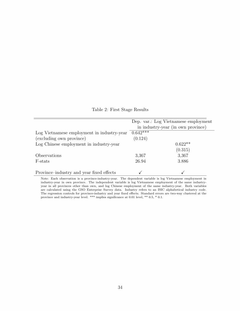
Table 2: First Stage Results

Dep. var.: Log Vietnamese employmentin industry-year (in own province)

Log Vietnamese employment in industry-year 0.642***(excluding own province) (0.124)Log Chinese employment in industry-year 0.622**

(0.315)Observations 3,367 3,367F-stats 26.94 3.886

Province–industry and year fixed effects X XNote: Each observation is a province-industry-year. The dependent variable is log Vietnamese employment inindustry-year in own province. The independent variable is log Vietnamese employment of the same industry-year in all provinces other than own, and log Chinese employment of the same industry-year. Both variablesare calculated using the GSO Enterprise Survey data. Industry refers to an ISIC alphabetical industry code.The regression controls for province-industry and year fixed effects. Standard errors are two-way clustered at theprovince and industry-year level. *** implies significance at 0.01 level, ** 0.5, * 0.1.

34

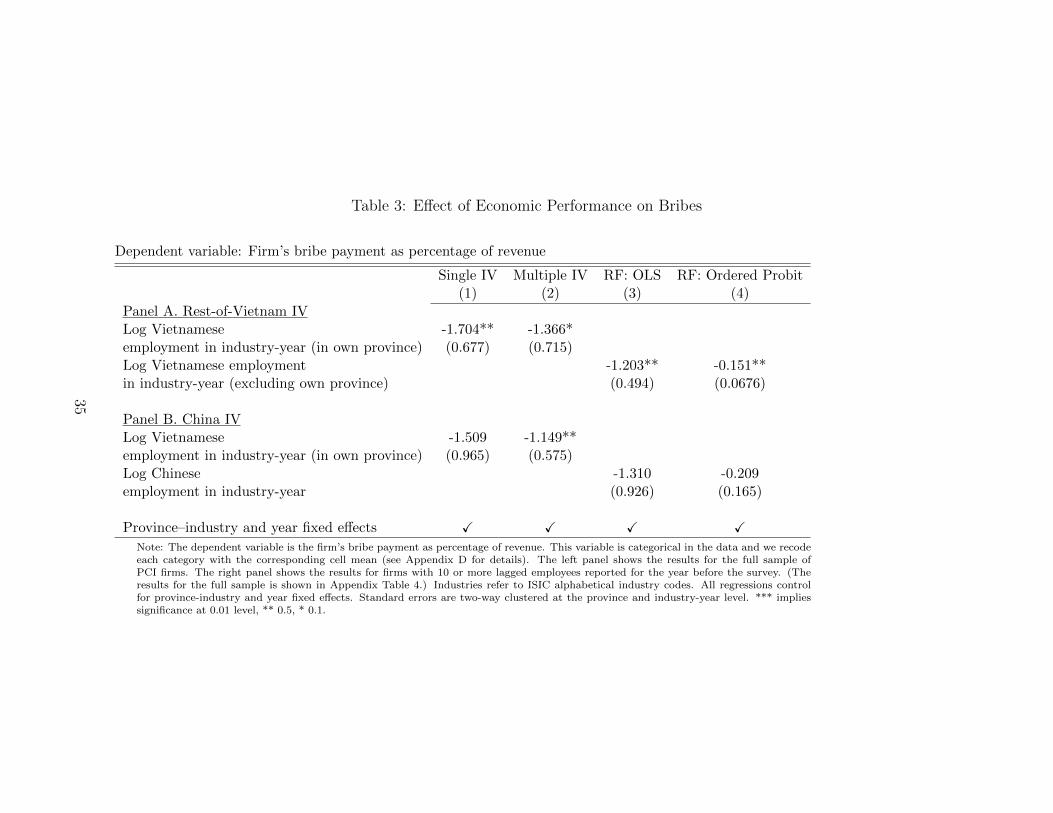
Table 3: Effect of Economic Performance on Bribes

Dependent variable: Firm’s bribe payment as percentage of revenue

Single IV Multiple IV RF: OLS RF: Ordered Probit(1) (2) (3) (4)

Panel A. Rest-of-Vietnam IVLog Vietnamese -1.704** -1.366*employment in industry-year (in own province) (0.677) (0.715)Log Vietnamese employment -1.203** -0.151**in industry-year (excluding own province) (0.494) (0.0676)

Panel B. China IVLog Vietnamese -1.509 -1.149**employment in industry-year (in own province) (0.965) (0.575)Log Chinese -1.310 -0.209employment in industry-year (0.926) (0.165)

Province–industry and year fixed effects X X X XNote: The dependent variable is the firm’s bribe payment as percentage of revenue. This variable is categorical in the data and we recodeeach category with the corresponding cell mean (see Appendix D for details). The left panel shows the results for the full sample ofPCI firms. The right panel shows the results for firms with 10 or more lagged employees reported for the year before the survey. (Theresults for the full sample is shown in Appendix Table 4.) Industries refer to ISIC alphabetical industry codes. All regressions controlfor province-industry and year fixed effects. Standard errors are two-way clustered at the province and industry-year level. *** impliessignificance at 0.01 level, ** 0.5, * 0.1.

35

Table 4: Heterogeneous Effects Based on Firms’ Property Rights

Dependent variable: Firm’s bribe payment as percentage of revenue

Single IV Multiple IV(1) (2) (3) (4) (5) (6) (7) (8)

Panel A. Rest-of-Vietnam IVLog Vietnamese employment in industry-year (in own province) -1.986** 0.978 -2.116** 0.978 -1.127 0.00315 -1.431** -0.0553

(0.843) (2.696) (0.902) (2.775) (0.688) (2.006) (0.645) (2.016)Firm owns its land -0.331* -0.340* -0.318** -0.317**X log Vietnamese employment in industry year (in own province) (0.180) (0.187) (0.125) (0.126)Firm owns land and has LURC -0.292** -0.314** -0.101 -0.119 -0.262*** -0.264*** -0.0882 -0.0915X log Vietnamese employment in industry year (in own province) (0.116) (0.128) (0.124) (0.133) (0.0900) (0.0911) (0.117) (0.119)Observations 9,535 9,535 9,535 9,535 9,535 9,535 9,535 9,535

Panel B. China IVLog Vietnamese employment in industry-year (in own province) -1.321 1.182 -1.098 0.744 -0.889 0.881 -1.174** 0.879

(1.376) (2.839) (1.305) (2.638) (0.606) (1.945) (0.560) (1.921)Firm owns its land -0.542*** -0.562*** -0.223* -0.223*X log Vietnamese employment in industry year (in own province) (0.165) (0.163) (0.132) (0.133)Firm owns land and has LURC -0.404*** -0.423*** -0.102 -0.104 -0.252** -0.257** -0.120 -0.126X log Vietnamese employment in industry year (in own province) (0.135) (0.151) (0.150) (0.152) (0.105) (0.107) (0.116) (0.119)Observations 9,535 9,535 9,535 9,535 9,535 9,535 9,535 9,535

Control for average firm size X log Vietnamese employment NO YES NO YES NO YES NO YESin industry-year (in own province)Province-industry and year fixed effects X X X X X X X X

Note: This table shows the IV results for heterogeneous effects based on firms’ property rights. The interaction term is the product of log Vietnamese employmentin industry-year in own province and firm-level property rights variables. Column 1 to 4 use single instrument, and column 5 to 8 use multiple instruments. Panel Ashows the results using rest-of-Vietnam IV, and Panel B shows results using China IV. All regressions control for the main effects of the property right variables, butonly the interaction coefficients are reported in this table. The even columns control for for average firm size in the industry interacted with the endogenous variable.The sample contains firms with 10 or more lagged employees reported for the year before the survey. (The results for the full sample is shown in Appendix Table5.) All regressions control for province-industry and year fixed effects. Standard errors are two-way clustered at the province and industry-year level. *** impliessignificance at 0.01 level, ** 0.5, * 0.1.

36

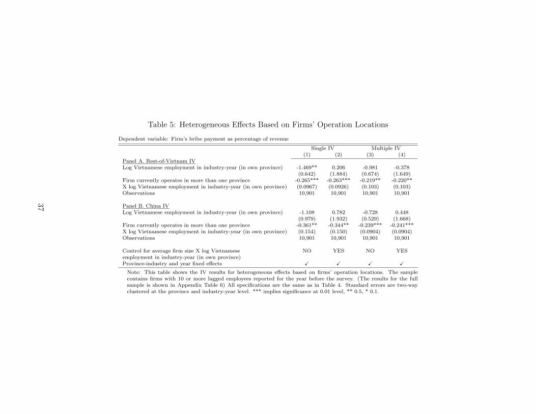
Table 5: Heterogeneous Effects Based on Firms’ Operation Locations

Dependent variable: Firm’s bribe payment as percentage of revenue

Single IV Multiple IV(1) (2) (3) (4)

Panel A. Rest-of-Vietnam IVLog Vietnamese employment in industry-year (in own province) -1.469** 0.206 -0.981 -0.378

(0.642) (1.884) (0.674) (1.649)Firm currently operates in more than one province -0.265*** -0.263*** -0.219** -0.220**X log Vietnamese employment in industry-year (in own province) (0.0967) (0.0926) (0.103) (0.103)Observations 10,901 10,901 10,901 10,901

Panel B. China IVLog Vietnamese employment in industry-year (in own province) -1.108 0.782 -0.728 0.448

(0.979) (1.932) (0.529) (1.668)Firm currently operates in more than one province -0.361** -0.344** -0.239*** -0.241***X log Vietnamese employment in industry-year (in own province) (0.154) (0.150) (0.0904) (0.0904)Observations 10,901 10,901 10,901 10,901

Control for average firm size X log Vietnamese NO YES NO YESemployment in industry-year (in own province)Province-industry and year fixed effects X X X X

Note: This table shows the IV results for heterogeneous effects based on firms’ operation locations. The samplecontains firms with 10 or more lagged employees reported for the year before the survey. (The results for the fullsample is shown in Appendix Table 6) All specifications are the same as in Table 4. Standard errors are two-wayclustered at the province and industry-year level. *** implies significance at 0.01 level, ** 0.5, * 0.1.

37

ONLINE APPENDICES FOR “FIRM GROWTH AND CORRUPTION”

• Appendix A: Additional tables

• Appendix B: Validation of matching between PCI and GSO

• Appendix C: Model

• Appendix D: Description of key variables

• Appendix E: Testing alternative models

38

Appendix A: Tables

Appendix Table 1: Cross-Validation of PCI and GSO Data

Firms with ≥ 10 lagged employees All firmsLog VN mean in PCI Log VN median in PCI Log VN mean in PCI Log VN median in PCI

(1) (2) (3) (4)Log VN mean in GSO 0.520*** 0.528***

(0.040) (0.033)Log VN median in GSO 0.474*** 0.440***

(0.045) (0.041)Observations 4484 4484 5760 5760

Province–industry and year FE X X X XNote: Each observation is a province-industry-year. The dependent variable is log mean or log median firm-level employment for each province-industry-year group inthe PCI data. The independent variable is the corresponding variable computed using the GSO data. For both datasets, we keep only private firms. Since the firmemployment variable in PCI is categorical, we compute the empirical mean and median for each category from the GSO data and apply these to the PCI data. Allspecifications control for province by industry (broad level) and year fixed effect. Robust standard errors are clustered at the province level and reported. *** impliessignificance at 0.01 level, ** 0.5, * 0.1.

39

Appendix Table 2: Industry Codes and Descriptions

ISIC Rev 4 Code DescriptionA Agriculture, forestry and fishingB Mining and quarryingC ManufacturingD Electricity, gas, steam and air conditioning supplyE Water supply; sewerage, waste management and remediation activitiesF ConstructionG Wholesale and retail trade; repair of motor vehicles and motorcyclesH Transportation and storageI Accommodation and food service activitiesJ Information and communicationK Financial and insurance activitiesL Real estate activitiesM Professional, scientific and technical activitiesN Administrative and support service activitiesP EducationQ Human health and social work activitiesR Arts, entertainment and recreationS Other service activities

The alphabetical industry codes and descriptions are based on International Standard Industrial Classification (ISIC) of AllEconomic Activities, Rev.4. The list includes the 18 industries that appear in our sample.

40

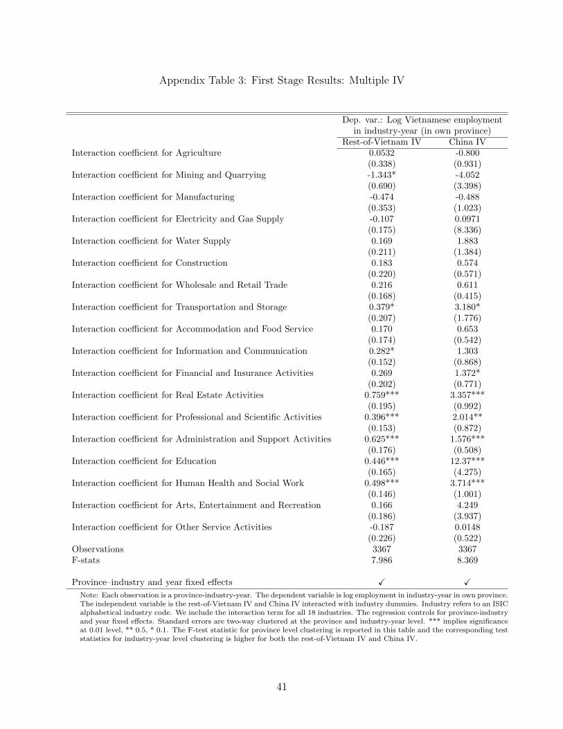
Appendix Table 3: First Stage Results: Multiple IV

Dep. var.: Log Vietnamese employmentin industry-year (in own province)

Rest-of-Vietnam IV China IVInteraction coefficient for Agriculture 0.0532 -0.800

(0.338) (0.931)Interaction coefficient for Mining and Quarrying -1.343* -4.052

(0.690) (3.398)Interaction coefficient for Manufacturing -0.474 -0.488

(0.353) (1.023)Interaction coefficient for Electricity and Gas Supply -0.107 0.0971

(0.175) (8.336)Interaction coefficient for Water Supply 0.169 1.883

(0.211) (1.384)Interaction coefficient for Construction 0.183 0.574

(0.220) (0.571)Interaction coefficient for Wholesale and Retail Trade 0.216 0.611

(0.168) (0.415)Interaction coefficient for Transportation and Storage 0.379* 3.180*

(0.207) (1.776)Interaction coefficient for Accommodation and Food Service 0.170 0.653

(0.174) (0.542)Interaction coefficient for Information and Communication 0.282* 1.303

(0.152) (0.868)Interaction coefficient for Financial and Insurance Activities 0.269 1.372*

(0.202) (0.771)Interaction coefficient for Real Estate Activities 0.759*** 3.357***

(0.195) (0.992)Interaction coefficient for Professional and Scientific Activities 0.396*** 2.014**

(0.153) (0.872)Interaction coefficient for Administration and Support Activities 0.625*** 1.576***

(0.176) (0.508)Interaction coefficient for Education 0.446*** 12.37***

(0.165) (4.275)Interaction coefficient for Human Health and Social Work 0.498*** 3.714***

(0.146) (1.001)Interaction coefficient for Arts, Entertainment and Recreation 0.166 4.249

(0.186) (3.937)Interaction coefficient for Other Service Activities -0.187 0.0148

(0.226) (0.522)Observations 3367 3367F-stats 7.986 8.369

Province–industry and year fixed effects X XNote: Each observation is a province-industry-year. The dependent variable is log employment in industry-year in own province.The independent variable is the rest-of-Vietnam IV and China IV interacted with industry dummies. Industry refers to an ISICalphabetical industry code. We include the interaction term for all 18 industries. The regression controls for province-industryand year fixed effects. Standard errors are two-way clustered at the province and industry-year level. *** implies significanceat 0.01 level, ** 0.5, * 0.1. The F-test statistic for province level clustering is reported in this table and the corresponding teststatistics for industry-year level clustering is higher for both the rest-of-Vietnam IV and China IV.

41

Appendix Table 4: Effect of Economic Performance on Bribes (All Firms)

Dependent variable: Firm’s bribe payment as percentage of revenue

Single IV Multiple IV RF: OLS RF: Ordered Probit(1) (2) (3) (4)

Panel A. Rest-of-Vietnam IVLog Vietnamese -1.890** -1.716**employment in industry-year (in own province) (0.770) (0.870)Log Vietnamese employment -1.389** -0.183**in industry-year (excluding own province) (0.619) (0.0837)

Panel B. China IVLog Vietnamese -2.017 -1.453**employment in industry-year (in own province) (1.285) (0.709)Log Chinese -1.454 -0.221employment in industry-year (0.909) (0.148)

Province–industry and year fixed effects X X X XNote: This table repeats the same regression analysis in Table 3 on the full sample of PCI firms (without size restriction). The correspondingRHS variable and IV are also constructed on the full sample firms in the GSO survey (aggregated to province-industry-year). *** impliessignificance at 0.01 level, ** 0.5, * 0.1.

42

Appendix Table 5: Heterogeneous Effects Based on Firms’ Property Rights (All Firms)

Dependent variable: Firm’s bribe payment as percentage of revenue

Single IV Multiple IV(1) (2) (3) (4) (5) (6) (7) (8)

Panel A. Rest-of-Vietnam IVLog Vietnamese employment in industry-year (in own province) -2.084** 0.497 -2.242** 0.464 -1.527* -0.110 -1.474* -0.186

(0.922) (2.526) (0.977) (2.622) (0.853) (1.914) (0.788) (1.919)Firm owns its land -0.442** -0.457** -0.410*** -0.410***X log Vietnamese employment in industry year (in own province) (0.188) (0.193) (0.130) (0.130)Firm owns land and has LURC -0.326*** -0.349*** -0.0709 -0.0865 -0.301*** -0.304*** -0.0821 -0.0853X log Vietnamese employment in industry year (in own province) (0.118) (0.129) (0.132) (0.137) (0.0813) (0.0829) (0.120) (0.121)Observations 9,588 9,588 9,588 9,588 9,588 9,588 9,588 9,588

Panel B. China IVLog Vietnamese employment in industry-year (in own province) -1.841 0.971 -1.487 0.606 -1.372* 0.546 -1.367** 0.505

(1.667) (3.758) (1.554) (3.106) (0.721) (1.805) (0.681) (1.798)Firm owns its land -0.602*** -0.661*** -0.295** -0.295**X log Vietnamese employment in industry year (in own province) (0.170) (0.216) (0.126) (0.125)Firm owns land and has LURC -0.412*** -0.449** -0.0739 -0.0667 -0.300*** -0.308*** -0.131 -0.138X log Vietnamese employment in industry year (in own province) (0.129) (0.188) (0.151) (0.145) (0.0977) (0.101) (0.118) (0.120)Observations 9,588 9,588 9,588 9,588 9,588 9,588 9,588 9,588

Control for average firm size X log Vietnamese employment NO YES NO YES NO YES NO YESin industry-year (in own province)Province-industry and year fixed effects X X X X X X X X

Note: This table repeats the same regression analysis in Table 4 on the full sample of PCI firms (without size restriction). The corresponding RHS variable and IV arealso constructed on the full sample firms in the GSO survey (aggregated to province-industry-year). *** implies significance at 0.01 level, ** 0.5, * 0.1.

43

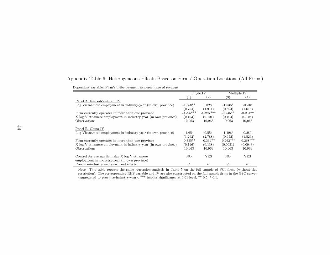
Appendix Table 6: Heterogeneous Effects Based on Firms’ Operation Locations (All Firms)

Dependent variable: Firm’s bribe payment as percentage of revenue

Single IV Multiple IV(1) (2) (3) (4)

Panel A. Rest-of-Vietnam IVLog Vietnamese employment in industry-year (in own province) -1.658** 0.0289 -1.536* -0.248

(0.754) (1.911) (0.824) (1.615)Firm currently operates in more than one province -0.295*** -0.297*** -0.246** -0.251**X log Vietnamese employment in industry-year (in own province) (0.103) (0.101) (0.104) (0.105)Observations 10,963 10,963 10,963 10,963

Panel B. China IVLog Vietnamese employment in industry-year (in own province) -1.654 0.554 -1.196* 0.289

(1.262) (2.788) (0.652) (1.526)Firm currently operates in more than one province -0.355** -0.334** -0.262*** -0.268***X log Vietnamese employment in industry-year (in own province) (0.146) (0.138) (0.0931) (0.0943)Observations 10,963 10,963 10,963 10,963

Control for average firm size X log Vietnamese NO YES NO YESemployment in industry-year (in own province)Province-industry and year fixed effects X X X X

Note: This table repeats the same regression analysis in Table 5 on the full sample of PCI firms (without sizerestriction). The corresponding RHS variable and IV are also constructed on the full sample firms in the GSO survey(aggregated to province-industry-year). *** implies significance at 0.01 level, ** 0.5, * 0.1.

44

Appendix Table 7: Robustness Check: Exclusion Restriction of the Rest-of-Vietnam IV

Dep. var: Bribe as % of revenueLog Vietnamese employment in industry-year -1.163**(excluding own region) (0.453)Constant 18.43***

(5.690)

Observations 10,898

Province-industry and year fixed effects XNote: This table reports the reduced form results using the alternative construction of the rest-of-Vietnam IV. In particular, we construct total employment in the same industry in other regions (asopposed to other provinces as in Table 3). The regression controls for province-industry and year fixedeffects. Standard errors are two-way clustered at the province and industry-year level. *** impliessignificance at 0.01 level, ** 0.5, * 0.1.

45

Appendix Table 8: Plausibly Exogenous Instruments: 95% Interval Estimates

(1) (2) (3)Coefficient 95CI lower bound 95CI upper bound

Main IV estimate (Column 1 Table 3) -1.704 -3.03 -0.38

Clustering s.e. at jt:δ=0 -3.4 -0.008δ=0.05 -3.059 -0.308δ=0.1 -2.802 -0.527δ=0.15 -2.546 -0.743δ=0.3 -1.792 -1.383δ=0.5 -2.216 -0.817

Clustering s.e. at r:δ=0 -3.37 -0.037δ=0.05 -3.033 -0.378δ=0.1 -2.798 -0.616δ=0.15 -2.565 -0.851δ=0.3 -1.882 -1.543δ=0.5 -2.43 -1.004

Note: This table presents 95% confidence intervals for the effect of economic performance on bribes using the “Union of CI”method proposed in Conley, Hansen, and Rossi (2012) across various prior settings. The “Union of CI” intervals impose theprior information that the support of γ, the direct impact of the instrument on the outcome, is [−2δ|β|, 2δ|β|], where β isour original IV estimate (-1.7 in column 1 of Table 3) and δ ranges from 0 to 0.5. In our main analysis, standard errors aretwo-way clustered at industry-year (jt) and region (r) level. For the plausibly exogenous tests, there isn’t a clear theoreticalguidance to perform the inference for two-way clustered standard errors. Therefore, we report the results for both ways. Foreach, we also report the IV estimate for γ = 0 (i.e., δ = 0).

46

Appendix Table 9: Heterogeneous Effects Based on Firms’ Property Rights (Contemporaneous Measure of LURC)

Dependent variable: Firm’s bribe payment as percentage of revenue

Rest-of-Vietnam Singe IV China Multiple IV(1) (2) (3) (4) (5) (6) (7) (8)

Log Vietnamese employment in industry-year -1.910** 1.046 -2.095** 1.055 -0.967 0.973 -1.260** 1.021(in own province) (0.840) (2.707) (0.904) (2.784) (0.599) (1.976) (0.585) (1.944)Firm owns its land X log Vietnamese employment -0.326* -0.350* -0.218 -0.222in industry year (in own province) (0.188) (0.203) (0.151) (0.153)Firm owns land and has LURC X log Vietnamese -0.309** -0.321** -0.0935 -0.0904 -0.263** -0.266** -0.114 -0.116employment in industry year (in own province) (0.140) (0.145) (0.164) (0.170) (0.120) (0.121) (0.155) (0.157)Observations 9,535 9,535 9,535 9,535 9,535 9,535 9,535 9,535

Control for average firm size X log Vietnamese NO YES NO YES NO YES NO YESemployment in industry-year (in own province)Province-industry and year fixed effects X X X X X X X X

Note: This table shows the IV results for heterogeneous effects based on firms’ property rights using contemporaneous Measure of LURC. The sample contains firms with10 or more lagged employees reported for the year before the survey.

47

Appendix Table 10: Heterogeneous Effects Based on Firms’ Property Rights (Ordered Probit)

Dependent variable: Firm’s bribe payment as percentage of revenue

Firms that rent Firms that own Firms that owntheir land land without LURC land with LURC

(1) (2) (3) (4) (5) (6)Log Vietnamese employment in industry-year -0.0402 0.923 -0.432*(excluding own province) (0.219) (0.573) (0.241)Log Chinese employment in industry-year -0.148 0.0210 -0.0379

(0.636) (0.813) (0.386)Observations 2,928 2,928 1,399 1,399 4,428 4,428

Province-industry and year fixed effects X X X X X XNote: This table reports the reduced form results using the ordered probit model for firms in three categories: (1) firms that rent their land; (2)firms that own land without an LURC; (3) firms that own land with an LURC. The sample contains firms with 10 or more lagged employeesreported for the year before the survey. All regressions control for province-industry and year fixed effects. Standard errors are two-way clusteredat the province and industry-year level. *** implies significance at 0.01 level, ** 0.5, * 0.1.

48

Appendix Table 11: Propensity Score Regressions for LURC and Operation Locations

Firm has Number of other provinces Firm currently operatesLURC in which firm operates in more than one province

(1) (2) (3)Share of registration documents held 0.605*** 0.511*** 0.490***

(0.098) (0.094) (0.091)Former HH firm (dummy) 0.432*** -0.058 -0.051

(0.056) (0.055) (0.054)Former SOE (dummy) 0.192** 0.250*** 0.275***

(0.092) (0.088) (0.085)Owner is government official (dummy) 0.440*** 0.391** 0.305**

(0.163) (0.153) (0.143)Government holds positive share (dummy) -0.354*** 0.116 0.115

(0.125) (0.118) (0.114)Log of business premise size (hectare) 0.264*** 0.024 0.027*

(0.018) (0.017) (0.016)Years since establishment 0.052*** 0.007* 0.009**

(0.005) (0.004) (0.004)Observations 7074 7872 7872

Note: Column 1 shows the logit regression coefficients of LURC (dummy) on various predictors of obtaining the certificate, including share of registrationdocuments held, former household firm (dummy), former SOE (dummy), owner being a government official (dummy), government holding positive share(dummy), log of business premise size, and firm’s age. Column 2 and 3 show the (ordered) logit regression results for firm’s operation location variableson the same set of explanatory variables. The sample contains firms with 10 or more lagged employees reported for the year before the survey. *** impliessignificance at 0.01 level, ** 0.5, * 0.1.

49

Appendix Table 12: Robustness Check: Heterogeneous Effects Based on Firms’ Property Rights (Single IV)

Dependent variable: Firm’s bribe payment as percentage of revenue

(1) (2) (3) (4) (5) (6) (7) (8)Includes characteristic [. . . ] and interaction with log Vietnamese employment in industry-year (in own province)

share of registration former former government government premise years of propensity scores for havingdocuments held HH firm SOE official share size establishment LURC and owning land

Panel A. Rest-of-Vietnam IVLog Vietnamese employment in industry-year 0.00285 1.023 0.841 1.226 1.011 0.650 1.135 1.377(in own province) (2.870) (2.772) (2.789) (2.807) (2.758) (3.044) (2.865) (2.951)Firm owns land and has LURC X log Vietnamese -0.102 -0.122 -0.116 -0.105 -0.119 -0.216 -0.0855 -0.130employment in industry year (in own province) (0.142) (0.130) (0.133) (0.130) (0.132) (0.156) (0.127) (0.164)Firm owns its land X log Vietnamese employment -0.438** -0.338* -0.349* -0.337* -0.342* -0.252 -0.373* -0.385*in industry year (in own province) (0.195) (0.190) (0.186) (0.183) (0.189) (0.207) (0.205) (0.212)Observations 7,671 9,534 9,534 9,534 9,534 8,874 9,347 7,074

Panel B. China IVLog Vietnamese employment in industry-year -0.623 0.695 0.639 1.193 0.813 1.476 0.671 1.080(in own province) (2.218) (2.658) (2.637) (2.845) (2.646) (2.264) (2.440) (2.737)Firm owns land and has LURC X log Vietnamese -0.0825 -0.0810 -0.0898 -0.0891 -0.103 -0.190 -0.0546 -0.120employment in industry year (in own province) (0.168) (0.145) (0.150) (0.153) (0.151) (0.183) (0.143) (0.209)Firm owns its land X log Vietnamese employment -0.682*** -0.601*** -0.570*** -0.575*** -0.566*** -0.517*** -0.592*** -0.695***in industry year (in own province) (0.174) (0.170) (0.165) (0.161) (0.165) (0.195) (0.178) (0.198)Observations 7,671 9,534 9,534 9,534 9,534 8,874 9,347 7,074

Control for average firm size X log Vietnamese YES YES YES YES YES YES YES YESemployment in industry-year (in own province)Province-industry and year fixed effects X X X X X X X X

Note: This table shows the single IV results for heterogeneous effects based on firms’ property rights after controlling for other firm characteristics. Column 1 to 8 controls for the followingexplanatory variables and their interactions with log Vietnamese employment in industry-year in own province: share of registration documents held, former household firm (dummy), formerSOE (dummy), owner being a government official (dummy), government holding positive share (dummy), log of business premise size, firm’s age, and the corresponding propensity score(s)for having LURC and/or owning land. The sample contains firms with 10 or more lagged employees reported for the year before the survey. All regressions control for the main effects ofthe property right variables, but only the interaction coefficients are reported in this table. All regressions control for province-industry and year fixed effects. Standard errors are two-wayclustered at the province and industry-year level. *** implies significance at 0.01 level, ** 0.5, * 0.1.

50

Appendix Table 13: Robustness Check: Heterogeneous Effects Based on Firms’ Property Rights (Multiple IV)

Dependent variable: Firm’s bribe payment as percentage of revenue

(1) (2) (3) (4) (5) (6) (7) (8)Includes characteristic [. . . ] and interaction with log Vietnamese employment in industry-year (in own province)

share of registration former former government government premise years of propensity scores for havingdocuments held HH firm SOE official share size establishment LURC and owning land

Panel A. Rest-of-Vietnam IVLog Vietnamese employment in industry-year 0.117 0.109 -0.386 0.0878 -0.0225 -0.320 0.0849 0.475(in own province) (2.356) (1.994) (1.985) (1.999) (2.003) (2.610) (2.039) (2.362)Firm owns land and has LURC X log Vietnamese -0.0855 -0.0896 -0.0835 -0.0751 -0.0837 -0.165 -0.0869 -0.128employment in industry year (in own province) (0.133) (0.119) (0.119) (0.117) (0.119) (0.138) (0.114) (0.157)Firm owns its land X log Vietnamese employment -0.372*** -0.323** -0.334*** -0.306** -0.316** -0.243* -0.341** -0.351***in industry year (in own province) (0.111) (0.131) (0.127) (0.126) (0.128) (0.143) (0.136) (0.136)Observations 7,671 9,534 9,534 9,534 9,534 8,874 9,347 7,074

Panel B. China IVLog Vietnamese employment in industry-year 0.647 1.051 0.564 1.109 0.917 0.795 1.110 0.970(in own province) (2.149) (1.926) (1.929) (1.930) (1.911) (2.159) (1.937) (2.236)Firm owns land and has LURC X log Vietnamese -0.115 -0.116 -0.125 -0.112 -0.121 -0.212 -0.117 -0.158employment in industry year (in own province) (0.134) (0.119) (0.118) (0.118) (0.118) (0.129) (0.113) (0.152)Firm owns its land X log Vietnamese employment -0.291** -0.243* -0.228* -0.214 -0.215 -0.128 -0.242* -0.229*in industry year (in own province) (0.123) (0.137) (0.131) (0.131) (0.134) (0.138) (0.138) (0.137)Observations 7,671 9,534 9,534 9,534 9,534 8,874 9,347 7,074

Control for average firm size X log Vietnamese YES YES YES YES YES YES YES YESemployment in industry-year (in own province)Province-industry and year fixed effects X X X X X X X X

Note: This table shows the multiple IV results for heterogeneous effects based on firms’ property rights after controlling for other firm characteristics (see footnote of Appendix Table 12).The sample contains firms with 10 or more lagged employees reported for the year before the survey. All regressions control for province-industry and year fixed effects. Standard errorsare two-way clustered at the province and industry-year level. *** implies significance at 0.01 level, ** 0.5, * 0.1.

51

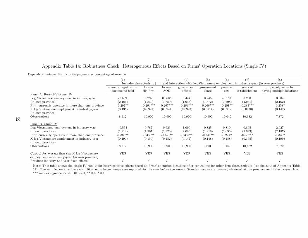
Appendix Table 14: Robustness Check: Heterogeneous Effects Based on Firms’ Operation Locations (Single IV)

Dependent variable: Firm’s bribe payment as percentage of revenue

(1) (2) (3) (4) (5) (6) (7) (8)Includes characteristic [. . . ] and interaction with log Vietnamese employment in industry-year (in own province)

share of registration former former government government premise years of propensity score fordocuments held HH firm SOE official share size establishment having multiple locations

Panel A. Rest-of-Vietnam IVLog Vietnamese employment in industry-year -0.539 0.292 0.0605 0.447 0.245 -0.158 0.230 0.804(in own province) (2.186) (1.859) (1.889) (1.943) (1.872) (1.708) (1.951) (2.162)Firm currently operates in more than one province -0.297** -0.264*** -0.267*** -0.263*** -0.266*** -0.201** -0.283*** -0.258*X log Vietnamese employment in industry-year (0.135) (0.0921) (0.0944) (0.0923) (0.0917) (0.0912) (0.0936) (0.142)(in own province)Observations 8,612 10,900 10,900 10,900 10,900 10,040 10,682 7,872

Panel B. China IVLog Vietnamese employment in industry-year -0.554 0.767 0.623 1.090 0.825 0.810 0.805 2.027(in own province) (1.914) (1.907) (1.920) (2.086) (1.919) (1.690) (1.943) (2.187)Firm currently operates in more than one province -0.383** -0.338** -0.343** -0.337** -0.345** -0.274* -0.367** -0.339*X log Vietnamese employment in industry-year (0.190) (0.150) (0.152) (0.147) (0.148) (0.158) (0.155) (0.199)(in own province)Observations 8,612 10,900 10,900 10,900 10,900 10,040 10,682 7,872

Control for average firm size X log Vietnamese YES YES YES YES YES YES YES YESemployment in industry-year (in own province)Province-industry and year fixed effects X X X X X X X X

Note: This table shows the single IV results for heterogeneous effects based on firms’ operation locations after controlling for other firm characteristics (see footnote of Appendix Table12). The sample contains firms with 10 or more lagged employees reported for the year before the survey. Standard errors are two-way clustered at the province and industry-year level.*** implies significance at 0.01 level, ** 0.5, * 0.1.

52

Appendix Table 15: Robustness Check: Heterogeneous Effects Based on Firms’ Operation Locations (Multiple IV)

Dependent variable: Firm’s bribe payment as percentage of revenue

(1) (2) (3) (4) (5) (6) (7) (8)Includes characteristic [. . . ] and interaction with log Vietnamese employment in industry-year (in own province)

share of registration former former government government premise years of propensity score fordocuments held HH firm SOE official share size establishment multiple locations

Panel A. Rest-of-Vietnam IVLog Vietnamese employment in industry-year -0.425 -0.307 -0.716 -0.0649 -0.404 -1.035 -0.405 1.391(in own province) (2.048) (1.574) (1.633) (1.738) (1.615) (2.184) (1.661) (2.133)Firm currently operates in more than one province -0.224* -0.209** -0.222** -0.220** -0.219** -0.163 -0.250** -0.203X log Vietnamese employment in industry-year (0.120) (0.102) (0.105) (0.101) (0.103) (0.104) (0.106) (0.130)(in own province)Observations 8,612 10,900 10,900 10,900 10,900 10,040 10,682 7,872

Panel B. China IVLog Vietnamese employment in industry-year 0.0657 0.481 0.0799 0.797 0.448 0.422 0.478 1.400(in own province) (2.010) (1.599) (1.659) (1.753) (1.629) (1.708) (1.645) (2.082)Firm currently operates in more than one province -0.242** -0.229*** -0.247*** -0.238*** -0.241*** -0.191** -0.273*** -0.205X log Vietnamese employment in industry-year (0.119) (0.0865) (0.0919) (0.0881) (0.0900) (0.0928) (0.0908) (0.126)(in own province)Observations 8,612 10,900 10,900 10,900 10,900 10,040 10,682 7,872

Control for average firm size X log Vietnamese YES YES YES YES YES YES YES YESemployment in industry-year (in own province)Province-industry and year fixed effects X X X X X X X X

Note: This table shows the multiple IV results for heterogeneous effects based on firms’ operation locations after controlling for other firm characteristics (see footnote of Table 12).The sample contains firms with 10 or more lagged employees reported for the year before the survey. Standard errors are two-way clustered at the province and industry-year level.*** implies significance at 0.01 level, ** 0.5, * 0.1.

53

Appendix Table 16: Testing Alternative Models

Herfindahl index for Bribes as % of revenue Bribes as % of revenueprovince-industry-year group (excluding construction industry)

(1) (2) (3)Log Vietnamese employment in industry-year 0.0421*** -1.744** -1.746***(in own province) (0.00319) (0.775) (0.629)Log Vietnamese province-year employment 0.884

(3.335)

Observations 2,780 9,001 10,901

Province-industry and year fixed effects X X XNote: This table shows the IV regression results for testing several alternative models. In Column 1, the dependent variable is the employment Herfindahl index constructedfor each province-industry-year group. The index is normalized to be between 0 and 1, where a small index indicates a competitive industry. For this regression, we keep 1observation per province-industry-year group. Column 2 shows the IV regression results using single rest-of-Vietnam IV where we exclude firms in the construction industry.For column 3, we include the province-year level total employment and instrument it using a predicted aggregate shock. In particular, the instrument is the weighted sum overall industries of industry-year employment in other provinces, normalized by the average over all years of total employment in the industry in other provinces. The weights arethe average over all years of industry’s share of employment in the given province. The sample contains firms with 10 or more lagged employees reported for the year before thesurvey. All regressions control for province-industry and year fixed effects. Standard errors are two-way clustered at the province and industry-year level. *** implies significanceat 0.01 level, ** 0.5, * 0.1.

54

Appendix B: Validation of matching between PCI and GSO

This section assesses the quality of the matching across data sets used in our analysis. Ideally,

we would have constructed our endogenous regressor (employment) using the same data set

that has our outcome (bribe) data. However, as discussed above, the PCI data, which has

information on bribes and firm mobility, is a sample, and does not include all firms. As

such, while the PCI is suitable for examining how a typical firm changes, we cannot use it

for accurately calculating aggregate shocks. For example, an increase in prices for goods sold

by industry j (one source of an increase in A) might lead to entry of firms, so even though

A increased, average firm size might decrease. For this reason, we use the GSO data, which

is a census, to construct our measure of A. However, before proceeding, it is important

to make sure that the PCI firms are a reasonably representative sample of all firms in the

GSO data, and that the industry codes we merge on are comparable across the data sets. If

not, then the reduced form results from regressing bribes as measured in the PCI data on

the GSO-based instrumental variable could be spurious, or null results could reflect poorly

matched data.

To cross-validate the two data sets and ensure that we are matching them appropriately,

we compare mean and median firm employment among private firms for each pjt group.

One issue with the PCI data is that employment is coded as a categorical variable: 10 to 50,

50 to 100, etc. To assign cardinal values to these bins, we compute the empirical mean and

median employment for all firms in GSO for each of these PCI bins, and use these values

to create the cardinal employment measure for the PCI firms. We then run the following

regression, with province-industry and year fixed effects:

log(EmployPCIpjt ) = α + β log(EmployGSO

pjt ) + νpj + µt + εpjt (7)

If the PCI firms are a perfect random sample of GSO firms, stratified by province, industry

and year, we should have β = 1. We report the estimates in Appendix Table 1. We can see

that the changes in mean employment in PCI and mean employment in GSO are positively

correlated: β is 0.520 and significant at the 1% level. Similarly, the median employment in

PCI and median employment in GSO are positively correlated and the coefficient is 0.474

and highly significant. The correlations are equally robust when we computed the mean and

median on the full sample of firms. These results confirm that, while the match between

the two data sets is not perfect, they are indeed comparable, even looking just over time at

changes within a given province-industry cell.

55

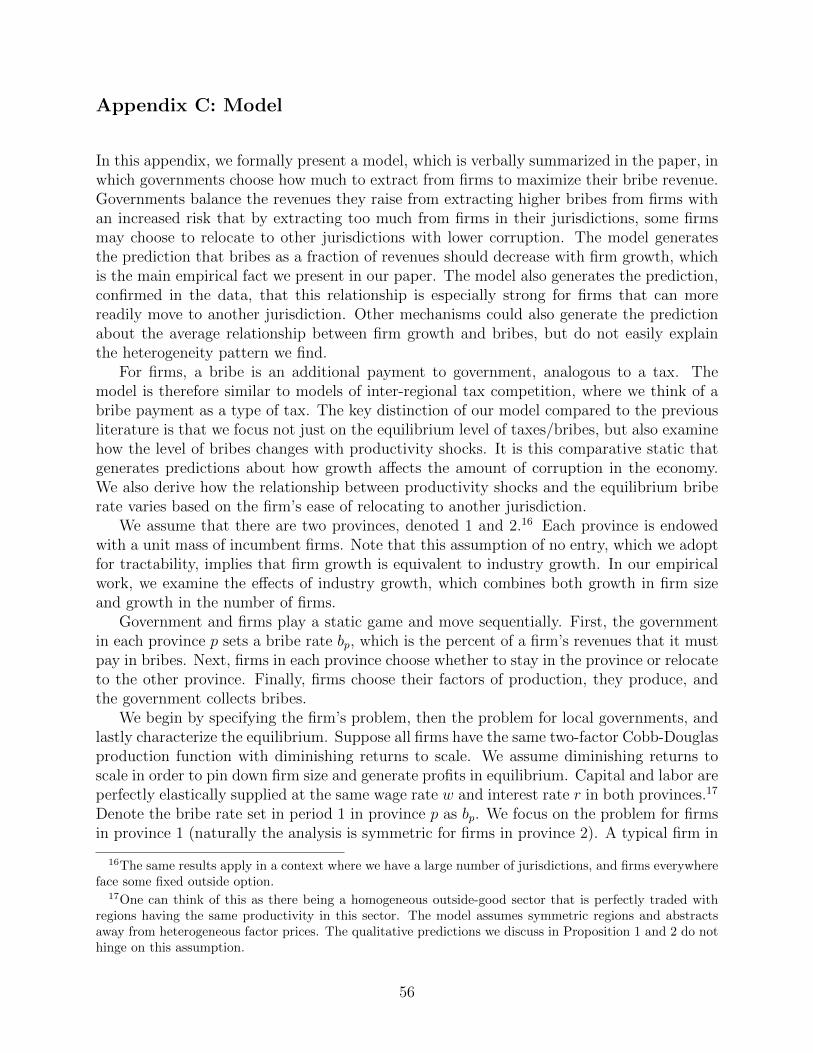
Appendix C: Model

In this appendix, we formally present a model, which is verbally summarized in the paper, inwhich governments choose how much to extract from firms to maximize their bribe revenue.Governments balance the revenues they raise from extracting higher bribes from firms withan increased risk that by extracting too much from firms in their jurisdictions, some firmsmay choose to relocate to other jurisdictions with lower corruption. The model generatesthe prediction that bribes as a fraction of revenues should decrease with firm growth, whichis the main empirical fact we present in our paper. The model also generates the prediction,confirmed in the data, that this relationship is especially strong for firms that can morereadily move to another jurisdiction. Other mechanisms could also generate the predictionabout the average relationship between firm growth and bribes, but do not easily explainthe heterogeneity pattern we find.

For firms, a bribe is an additional payment to government, analogous to a tax. Themodel is therefore similar to models of inter-regional tax competition, where we think of abribe payment as a type of tax. The key distinction of our model compared to the previousliterature is that we focus not just on the equilibrium level of taxes/bribes, but also examinehow the level of bribes changes with productivity shocks. It is this comparative static thatgenerates predictions about how growth affects the amount of corruption in the economy.We also derive how the relationship between productivity shocks and the equilibrium briberate varies based on the firm’s ease of relocating to another jurisdiction.

We assume that there are two provinces, denoted 1 and 2.16 Each province is endowedwith a unit mass of incumbent firms. Note that this assumption of no entry, which we adoptfor tractability, implies that firm growth is equivalent to industry growth. In our empiricalwork, we examine the effects of industry growth, which combines both growth in firm sizeand growth in the number of firms.

Government and firms play a static game and move sequentially. First, the governmentin each province p sets a bribe rate bp, which is the percent of a firm’s revenues that it mustpay in bribes. Next, firms in each province choose whether to stay in the province or relocateto the other province. Finally, firms choose their factors of production, they produce, andthe government collects bribes.

We begin by specifying the firm’s problem, then the problem for local governments, andlastly characterize the equilibrium. Suppose all firms have the same two-factor Cobb-Douglasproduction function with diminishing returns to scale. We assume diminishing returns toscale in order to pin down firm size and generate profits in equilibrium. Capital and labor areperfectly elastically supplied at the same wage rate w and interest rate r in both provinces.17

Denote the bribe rate set in period 1 in province p as bp. We focus on the problem for firmsin province 1 (naturally the analysis is symmetric for firms in province 2). A typical firm in

16The same results apply in a context where we have a large number of jurisdictions, and firms everywhereface some fixed outside option.

17One can think of this as there being a homogeneous outside-good sector that is perfectly traded withregions having the same productivity in this sector. The model assumes symmetric regions and abstractsaway from heterogeneous factor prices. The qualitative predictions we discuss in Proposition 1 and 2 do nothinge on this assumption.

56

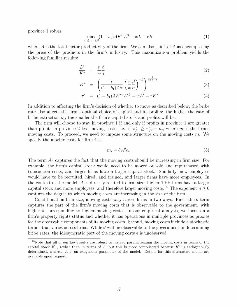
province 1 solvesmax

K≥0,L≥0(1− b1)AKαLβ − wL− rK (1)

where A is the total factor productivity of the firm. We can also think of A as encompassingthe price of the products in the firm’s industry. This maximization problem yields thefollowing familiar results:

L∗

K∗=

r

w

β

α(2)

K∗ =

(r

(1− b1)Aα

(r

w

β

α

)−β) 1α+β−1

(3)

π∗ = (1− b1)AK∗αL∗β − wL∗ − rK∗ (4)

In addition to affecting the firm’s decision of whether to move as described below, the briberate also affects the firm’s optimal choice of capital and its profits: the higher the rate ofbribe extraction b1, the smaller the firm’s capital stock and profits will be.

The firm will choose to stay in province 1 if and only if profits in province 1 are greaterthan profits in province 2 less moving costs, i.e. if π∗f1 ≥ π∗f2 − m, where m is the firm’smoving costs. To proceed, we need to impose some structure on the moving costs m. Wespecify the moving costs for firm i as

mi = θAηεi. (5)

The term Aη captures the fact that the moving costs should be increasing in firm size. Forexample, the firm’s capital stock would need to be moved or sold and repurchased withtransaction costs, and larger firms have a larger capital stock. Similarly, new employeeswould have to be recruited, hired, and trained, and larger firms have more employees. Inthe context of the model, A is directly related to firm size; higher TFP firms have a largercapital stock and more employees, and therefore larger moving costs.18 The exponent η ≥ 0captures the degree to which moving costs are increasing in the size of the firm.

Conditional on firm size, moving costs vary across firms in two ways. First, the θ termcaptures the part of the firm’s moving costs that is observable to the government, withhigher θ corresponding to higher moving costs. In our empirical analysis, we focus on afirm’s property rights status and whether it has operations in multiple provinces as proxiesfor the observable components of its moving costs. Second, moving costs include a stochasticterm ε that varies across firms. While θ will be observable to the government in determiningbribe rates, the idiosyncratic part of the moving costs ε is unobserved.

18Note that all of our key results are robust to instead parameterizing the moving costs in terms of thecapital stock K∗, rather than in terms of A, but this is more complicated because K∗ is endogenouslydetermined, whereas A is an exogenous parameter of the model. Details for this alternative model areavailable upon request.

57

Putting the pieces together, a firm in province 1 chooses to stay if and only if

π∗1 ≥ π∗2 − θAηε, or

ε ≥ π∗2 − π∗1θAη

(6)

To simplify the algebra, we further assume that ε is uniformly distributed over [0, 1].19 The

equilibrium number of firms for a given θ in province 1 is therefore simply 1− π∗2−π∗

1

θAη .20 Sincethe problem is symmetric for both provinces, this expression will be greater than 1 if b1 < b2

(firms are moving into province 1 from province 2), and less than 1 if b1 > b2 (firms aremoving out of province 1 to province 2).

The two governments in period 1 set bribe rates, taking firms’ response and the otherprovince’s bribe rate as given. To solve this, we consider the government in province 1. Ittakes b2 as given and solves,

maxb1≥0

b1AK∗αL∗β

(1− π∗2 − π∗1

θAη

)(7)

Assuming a symmetric equilibrium, the first-order condition can be simplified to:

K∗ + b∗1(α + β)dK∗

db1

+b∗1K

∗

θAηdπ∗1db1

= 0 (8)

After some algebra, we get:(1

θA1−η

(rβ

wα

)βK∗α+β +

α + β

1− α− β1

1− b∗

)b∗ = 1 (9)

Note that we have suppressed the province subscript since b∗1 = b∗2 in equilibrium.Several aspects of the equilibrium condition in Equation (9) are worth noting. First,

as θ goes to +∞, or firms are completely immobile, the expression simplifies such thatb∗ = 1 − α − β. This implies that the greater the diminishing returns to scale, the higherthe bribe rate. Intuitively, if output is highly concave in capital, even when the bribe rate isreduced, firms will not expand their capital stock much due to diminishing returns. Thus,the elasticity of capital with respect to the bribe rate is low. The same applies to labor.Therefore, when the government increases the bribe rate, it can extract more revenue fromfirms without discouraging production. Hence, the optimal bribe rate is higher.

The second observation is that as θ decreases, so that moving costs decrease, inter-regional competition increases and the equilibrium bribe rate decreases. Thus far, the modelcaptures the idea that increasing competition between political jurisdictions can drive downcorruption, as in Shleifer and Vishny (1993) and Burgess et al. (2012).

19This assumption simplifies the algebra but is not essential; all of the key results go through for arbitrarydistributional forms of the error term.

20Even though we have in mind a world of many firms with heterogenous θ, we are solving the model fora particular θ. After we obtain the equilibrium bribe rate, which is a function of θ, we will examine howbribes and the effect of firm growth on bribes vary with θ.

58

Next, we examine how the equilibrium bribe rate responds to increases in the productivityof firms, i.e. increases in A. Taking the derivative with respect to logA on both sides ofEquation (9) and re-arranging terms, we get our first result:

Proposition 1. db∗

d logA< 0 if 0 ≤ η < 1

1−α−β ; = 0 if η = 11−α−β ; and > 0 if η > 1

1−α−β .

Proof. : One way to prove the results is using standard first order condition and tak-ing derivative by invoking implicit function theorem. Here we first make a transforma-tion of variables to simplify the problem. First notice that by replacing K,L,A, θ byrK,wL, A

rαwβ , θ(rαwβ)η, we can assume w = r = 1 without changing the problem. This

linear change of variable also preserves the signs of the derivatives in question.We can rewrite the firm’s objective function:

π∗1 = maxK,L≥0(1− b1)AKαLβ −K − L

which gives

K∗1 = α((1− b1)Aααββ)1

1−α−β

L∗1 = β((1− b1)Aααββ)1

1−α−β

π∗1 = (1− α− β)((1− b1)Aααββ)1

1−α−β

Substituting these into the government’s problem, we are able to calculate the total bribereceived by government in province 1:

B1 = t(1− λ(R2 −R1))(Rα+β1 −R1) (10)

where

R1 = (1− b1)1

1−α−β (11)

R2 = (1− b2)1

1−α−β (12)

λ =A

11−α−β

θAη(1− α− β)(ααββ)

11−α−β (13)

t = (Aααββ)1

1−α−β (14)

Instead of choosing b1, b2 ∈ (0, 1), the two provinces could choose R1, R2 ∈ (0, 1) as well.The FOC for (10) then yields

λ(Rα+β1 −R1) = (1− λ(R2 −R1)) ∗ (1− (α + β)Rα+β−1

1 ) (15)

The symmetric equilibrium R1 = R2 = R∗ must then satisfy

λ(Rα+β1 −R1) = 1− (α + β)Rα+β−1

1 (16)

This gives the equilibrium bribe rate b∗ via (11).With that preliminary math completed, we can complete the proof. Re-arrange (16) and

59

notice that the ratio

φ :=1− (α + β)Rα+β−1

1

(Rα+β1 −R1)

is strictly increasing in R, because Rα+β1 −R1 is concave and hence log-concave in R. There-

fore, (16) has a unique solution for fixed parameters (so fixed λ), and this solution is strictlyincreasing in λ. In other words,

dR∗

dλ> 0 (17)

From (11), b∗ = 1−(R∗)1−α−β, and so db∗

dR∗ < 0. Also from (13), dλdA

is positive when η < 11−α−β

and negative otherwise. Multiplying the three inequalities, we obtain

db∗

dA> 0,when η >

1

1− α− βdb∗

dA< 0,when η <

1

1− α− β

The critical factor that determines the sign of db∗/d logA is η, which characterizes theconcavity of the moving costs with respect to the capital stock. The intuition is that witha positive shock to A, for a given size, firms enjoy higher revenues and hence care moreabout the bribes they will pay and less about the moving costs. This tends to drive downthe equilibrium bribe rate due to inter-regional competition. However, at the same time,the cost of moving rises as firms expand in size to take advantage of the higher productivity.This instead tends to drive up the equilibrium bribe rate. The two effects exactly cancel atη = 1

1−α−β .21 If η < 11−α−β , then the first effect (inter-regional competition effect) dominates

the second effect (moving cost effect), and the equilibrium bribe rate falls. Given that1 − α − β < 1, a sufficient condition for db∗

d logA< 0 is that moving costs scale up less than

linearly with firm size, as proxied by A. Moving costs seem likely to fulfill this assumption inpractice and, moreover, because 1−α−β can in fact be much less than 1, it seems plausiblethat η < 1

1−α−β and therefore db∗/d logA < 0 in most settings. The empirical evidencepresented in the previous section matches this prediction of the model.

Proposition 1 specifies conditions when the rate of bribe extraction falls as A increases;the rate b is the size of the distortion to production. It is worth noting that another (testable)prediction is that the total amount of bribes extracted from the firm will increase when Aincreases. To see this note that the firm’s moving decision is a tradeoff between its totalmoving costs and its total bribes. Since when A increases, the firm’s moving costs increase,the government can retain the same firms even with a higher total bribe extraction.

Also worth noting is that to the extent that taxes follow similar patterns to bribes,another implication of the model is that taxes on firms should also be lower in rich countriesthan in poor countries. There is suggestive evidence along these lines: Gordon and Li

21Though the specific cut-off value for η at which the sign of the comparative statics switches depends onthe Cobb-Douglas functional form for production and the particular parameterization of the moving costs,the general intuition is robust: The more concave the moving costs with respect to firm size are, the morelikely that equilibrium bribe rate decreases with A.

60

(2009) show that for poor countries (with per-capita GDP below $745), corporate incometaxes represent 7.5 percent of GDP, whereas for rich countries (with per-capita GDP above$9,200), corporate income taxes represent only 4.5 percent of GDP, although they suggest adifferent explanation than the one proposed here.

Next, we examine how the effect of a productivity shock on bribes varies across firms withdifferent θ. We will focus on the firm’s property right status or multi-province operations asthe empirical analogue of θ, where higher θ corresponds to less transferable property rightsor concentration of operations in one province and thus a higher cost of moving. The nextproposition derives how the elasticity of bribes with respect to productivity varies with θ.

Proposition 2. The elasticity −d log b∗

d logAis monotonically decreasing in θ if and only if 0 ≤

η < 11−α−β . That is, d2 log b∗

d logAdθ> 0 iff 0 ≤ η < 1

1−α−β .

Proof. : From (11),

εR∗ =1

1− α− βb∗

1− b∗εb∗ (18)

where εR = dRdA

AR

and εb = − dbdA

Ab. Taking the derivative of (16) with respect to A, we get

(omitting stars)

ελ :=1

1− α− β− η =

((α + β)(1− α− β)Rα+β−1

1− (α + β)Rα+β−1+R− (α + β)Rα+β

Rα+β −R

)εR (19)

Substitute (18) and (11) into (19), we have

ελεb

=

((α + β)Rα+β−2 +

Rα+β−1 − 1

(1− α− β)R

)φ−1 (20)

It is easy to see that b∗ (R∗) increases (decreases) with θ, and thus the right hand sideincreases with θ. Therefore,

dεb∗

dθ< 0,when ελ > 0⇔ η <

1

1− α− β(21)

Intuitively, Proposition 1 implied that bribes fall when there is an increase in A, becausemore profitable firms are more willing to pay moving costs and escape from high bribe rates.Proposition 2 states that the bribe rate falls more after such a shock for firms with lowerobservable moving costs because the fraction of firms who are on the margin of moving islarger, so a given change in bribes will induce a larger number of them to leave.22

22Note that Proposition 2 is stated in terms of elasticity or percentage change in the bribe rate (i.e. the

change in log b). The sign for the cross-partial of the level change (ie. d2b∗

dAdθ ) is in general indeterminantbecause though the elasticity falls with θ (under the condition in Proposition 2), the level of bribe also fallswith θ. In particular, we can show that the relationship between db∗

dA and θ is U-shaped and increasing as

θ →∞, and d2b∗

dAdθ > 0 for a reasonable range of θ as assessed by the ratio of moving costs to revenue.

61

Appendix D: Description of key variables

The key variables described in Table 1 are below. Note that each observation is a firm; thesample pools firms for the years 2006 to 2010. The PCI firms in our sample are firms with atleast 10 employees, valid industry and bribe payment data and whose province-industry-yearis represented in the GSO data.

• Bribes as percentage of revenue (PCI): This is a 7-point categorical variable drawnfrom question D6 of the annual PCI survey. Respondents answered within ranges: 1)0%; 2) less than 1%; 3) 1-2%; 4) 2-10%; 5) 10-20%; 6) 20-30%; 7) over 30%. We recodeeach category with the corresponding cell mean with over 30% recoded as 35%.

• Years since establishment (PCI): Continuous variable that subtracts year of establish-ment from the year the firm completed the survey (2006 to 2010). Establishment onlycaptures when the firm began doing business and has no legal connotation. A follow-upquestion asks when a firm registered as a formal business.

• Number of employees (PCI): This variable is categorical in PCI: for example, 10-49,50-199, etc. We recode each category with the corresponding empirical cell mean inGSO.

• Mean employment (GSO, mean for industry-year-province level): Continuous measurecollected in the GSO Enterprise Census.

• Log employment (GSO, aggregate for industry-year-province): Continuous measurecollected in the GSO Enterprise Census.

• Log of business premise size (hectares) (PCI): Continuous measure collected in onlythe 2009 to 2011 surveys.

• Land ownership (dummy) (PCI): Dichotomous variable measuring whether a firm pur-chased (=1) or leases (=0) its main business premises.

• Land use right certificate (LURC, dummy) (PCI): Dichotomous variable measuringwhether a firm possesses an LURC for its main business premises.

• Land ownership without land use right certificate (dummy) (PCI): Dichotomous vari-able, calculated from questions about whether a firm owns land and whether it has anLURC for that land.

• Number of other provinces in which firm operates (PCI): Count variable calculatedfrom firm’s response to a question asking it to record all provinces and national-levelcities in which it has operations or branch offices, outside of its headquarters location.

• Firm currently operates in more than one province (dummy) (PCI): Dichotomous vari-able for whether firm listed operations in at least one province outside the provincewith its main headquarters.

62

• Share of registration documents held: Based on the following question: “In addition tothe certificate of business registration, your business may need additional permits orbusiness to be fully legal (e.g. mining licenses....). How many of these documents wererequired for your firm?’ “Y” Variable defined as the number of registration documentsheld by the firm divided by the 95% percentile of the firm’s industry (a proxy forformality).

• Former household firm (dummy) (PCI): Dichotomous variable for whether the firm op-erated as an informal business based on household premises before formal registration.

• Former SOE (dummy) (PCI): Based on questions asking whether the firm is a priva-tized former State Owned Enterprise (SOE). Equals 1 if the firm is either a locally orcentrally managed SOE.

• Owner is a former government official (dummy) (PCI): Based on question askingwhether the owner of the private enterprise is a former government official, army office,or SOE manager.

• Government holds a positive share (dummy) (PCI): Based on question asking whethershares of the firm are held by local or central government officials.

63

Appendix E: Testing alternative models

Empirical confirmation of several predictions of our model supports the idea that inter-jurisdictional competition is a mechanism through which economic growth can reduce bribery.However, there are also other potential models that predict a negative correlation of eco-nomic growth and the bribe rate. The first and most direct way to distinguish between theinter-jurisdictional model and these other models is that we find that the relationship be-tween growth and bribery is diminished for firms that are less likely to relocate outside theirprovince. This is a direct prediction of inter-jurisdictional competition, but is not predictedby most other models.

Nonetheless, it is possible that these heterogenous effects are picking up other firm char-acteristics besides property rights or multiple locations. Thus, it is important to considerseveral other possible explanations for the general pattern that economic growth reducesbribes, and to discuss the degree to which our evidence is, or is not, consistent with them.

Product-market competition

Economic growth could increase competition among firms, and this product market compe-tition affects the amount of rents bureaucrats can capture. If firms have less market powerand smaller rents, then bureaucrats may be less able to extract bribes from them. Ades andDi Tella (1999) present empirical evidence that product market competition reduces corrup-tion, for example. To probe the possibility of this mechanism, we test the starting premisethat the variation in economic growth that we analyze increases market competition. Weregress the Herfindahl index, constructed using employment (our most accurate measure offirm size) from the GSO data, on employment, instrumented with industry employment inthe rest of Vietnam (log(Employp−jt)). We find that higher predicted employment leadsto less, not more, competition, suggesting that the main mechanism through which growthreduces bribery in our context is not increased firm competition (Appendix Table 16, col-umn 1).23 However, Bliss and Di Tella (1997) present a model in which, counterintuitively,less competition among firms can lead to less bribery; it is possible that this mechanismof reduced competition among firms (higher rents for firms) leading to a reduction in bribeextraction is at play in our setting.

Spurious effect of industry-specific bribe crackdowns

A second possibility we consider is that there are industry-specific crackdowns on bribes. Asdiscussed earlier, this represents the fundamental identification assumption of the within-Vietnam analysis: There are no industry-specific crackdowns on bribes. The strongest evi-dence in support of our assumption is that when we use industry size in China to instrumentfor industry size in Vietnam, we find similar results, suggesting that internal reverse causalitywithin Vietnam is not driving the results.

23Another option would be to test for changes in profit margins directly. However, the profit margin datain the GSO is known to be much less reliable than employment (Tran and Dao, 2013), as firms routinelyunderreport profits to avoid taxes. For example, in the GSO data, 38 percent of firms report a profit marginof less than 1 percent of revenues, with 23 percent of firms reporting 0 profits. Given these reporting issues,the PCI dataset does not ask about profits.

64

Moreover, the institutional structure of Vietnam, which we described in section 2.1 issuch that bribery is decentralized to the province level, suggesting that national industry-level crackdowns are unlikely (recall that our identifying variation is essentially Vietnam-wide growth for an industry). In addition, we undertook a systematic review of the nationalanti-corruption website, which documents major anti-corruption efforts of the government.Over the study period, only one industry-specific anti-corruption campaign is documented, acrackdown in the construction industry in 2008. Appendix Table 16, column 2 shows that themain results are essentially unchanged when we re-run our main specification from column1 of Table 3, but excluding the construction industry. As the fundamental identificationassumption, it is difficult to establish empirically that there are no industry-specific shocksto bribes, but the qualitative evidence points against such an explanation for the patternswe find.

Fixed cost of anti-corruption enforcement

Another possibility is that there is a layer of oversight over bureaucrats aimed at rooting outcorruption, such as an anti-corruption agency. The overseers face a fixed cost of enforcement,so as the total scale of bribery (in levels) goes up, it is easier to detect and punish bribery.Or said differently, it may be easier to detect a larger bribe. If so, then as firms grow,bureaucrats will adjust the bribe rate down.

While this explanation may be at work at the cross-country level, it does not seem tobe a key factor explaining the results in this paper. In particular, since most regulatoryactivities are at the province level, if fixed costs were the main explanation, then the keyfactor determining bribes would be the overall size of economic activity in the province as awhole, not the size of particular industries.

To test this, column 3 of Appendix Table 16 reruns the main IV regression, but inaddition to including log employment in a province-year in the particular industry, we alsoinclude the aggregate endogenous variable, which is log employment in the province-yearin all industries. Because we have two endogenous regressors, we need two instruments.For the first, we use our standard single IV that is industry-year employment in the rest ofVietnam. The second IV aggregates employment across all industries in the rest of Vietnam.To construct this aggregate instrument, we calculate the log of the weighted sum over allindustries of employment in the industry in a given year in all provinces excluding provincep itself (relative to the average over all years), where the weights represent the share of totalemployment in province p that comes from industry j. Specifically, define the weights foreach industry j in province p as:

wpj =1

T

∑t

EmploypjtEmploypt

. (22)

65

Then the predicted log employment in province p at time t is:

predicted log(Employpt) = log

∑j

wpjEmployp−jt(

1

T

∑tEmployp−jt

) (23)

where the1

T

∑tEmployp−jt term is a normalization such that the weights to each industry

are given exactly by wpj. Note that with a single industry j in a province, predicted log(Employpt)reduces exactly to log(Employp−jt).

Using this approach, the evidence in column 3 suggests that, the IV coefficient estimateon overall province employment, log(Employpt), is insignificant, and the negative coefficienton industry-specific log(Employpjt) is unchanged from our main specification. This suggeststhat the results are not being driven by aggregate changes in enforcement practices at theprovince level.

Diminishing returns to bribes

A final alternative explanation for the main effect we find is that bureaucrats have dimin-ishing marginal utility of income relative to the risk of being caught and going to jail. Thus,as it becomes easier to extract a given amount of bribe revenues, they reduce the rate. Thereduced form effect of this mechanism would be similar to a fixed cost of anti-corruptionenforcement within each province: A decline in bribes would be driven by aggregate em-ployment in the province, not industry-specific employment. The results in column 3 ofAppendix Table 16 suggest that this is not the entire explanation for our results.

Summary

In summary, to the extent we can examine quantitative and qualitative predictions of thesealternative models, we do not find that other mechanisms can explain all the facts in thedata. It still may well be that these other mechanisms are in operation and explain someof the overall effect of growth on bribery. But, the positive evidence in support of inter-jurisdictional competition and the limited evidence in support of other models suggests thatthe mechanism we highlight is at least one important factor in why economic growth reducescorruption in Vietnam.

66