fire detection algorithms using multimodal...
TRANSCRIPT

FIRE DETECTION ALGORITHMS USINGMULTIMODAL SIGNAL AND IMAGE
ANALYSIS
a dissertation submitted to
the department of electrical and electronics
engineering
and the institute of engineering and science
of bIlkent university
in partial fulfillment of the requirements
for the degree of
doctor of philosophy
By
Behcet Ugur Toreyin
January, 2009

I certify that I have read this thesis and that in my opinion it is fully adequate,
in scope and in quality, as a dissertation for the degree of doctor of philosophy.
Prof. Dr. A. Enis Cetin (Supervisor)
I certify that I have read this thesis and that in my opinion it is fully adequate,
in scope and in quality, as a dissertation for the degree of doctor of philosophy.
Prof. Dr. Orhan Arıkan
I certify that I have read this thesis and that in my opinion it is fully adequate,
in scope and in quality, as a dissertation for the degree of doctor of philosophy.
Assoc. Prof. Dr. A. Aydın Alatan
ii

I certify that I have read this thesis and that in my opinion it is fully adequate,
in scope and in quality, as a dissertation for the degree of doctor of philosophy.
Assoc. Prof. Dr. Ugur Gudukbay
I certify that I have read this thesis and that in my opinion it is fully adequate,
in scope and in quality, as a dissertation for the degree of doctor of philosophy.
Asst. Prof. Dr. Sinan Gezici
Approved for the Institute of Engineering and Science:
Prof. Dr. Mehmet B. BarayDirector of the Institute
iii

ABSTRACT
FIRE DETECTION ALGORITHMS USINGMULTIMODAL SIGNAL AND IMAGE ANALYSIS
Behcet Ugur Toreyin
Ph.D. in Electrical and Electronics Engineering
Supervisor: Prof. Dr. A. Enis Cetin
January, 2009
Dynamic textures are common in natural scenes. Examples of dynamic tex-
tures in video include fire, smoke, clouds, volatile organic compound (VOC)
plumes in infra-red (IR) videos, trees in the wind, sea and ocean waves, etc.
Researchers extensively studied 2-D textures and related problems in the fields
of image processing and computer vision. On the other hand, there is very little
research on dynamic texture detection in video. In this dissertation, signal and
image processing methods developed for detection of a specific set of dynamic
textures are presented.
Signal and image processing methods are developed for the detection of flames
and smoke in open and large spaces with a range of up to 30m to the camera
in visible-range (IR) video. Smoke is semi-transparent at the early stages of fire.
Edges present in image frames with smoke start loosing their sharpness and this
leads to an energy decrease in the high-band frequency content of the image.
Local extrema in the wavelet domain correspond to the edges in an image. The
decrease in the energy content of these edges is an important indicator of smoke
in the viewing range of the camera. Image regions containing flames appear as
fire-colored (bright) moving regions in (IR) video. In addition to motion and
color (brightness) clues, the flame flicker process is also detected by using a Hid-
den Markov Model (HMM) describing the temporal behavior. Image frames are
also analyzed spatially. Boundaries of flames are represented in wavelet domain.
High frequency nature of the boundaries of fire regions is also used as a clue to
model the flame flicker. Temporal and spatial clues extracted from the video are
combined to reach a final decision.
iv

v
Signal processing techniques for the detection of flames with pyroelectric (pas-
sive) infrared (PIR) sensors are also developed. The flame flicker process of an
uncontrolled fire and ordinary activity of human beings and other objects are
modeled using a set of Markov models, which are trained using the wavelet trans-
form of the PIR sensor signal. Whenever there is an activity within the viewing
range of the PIR sensor, the sensor signal is analyzed in the wavelet domain and
the wavelet signals are fed to a set of Markov models. A fire or no fire decision is
made according to the Markov model producing the highest probability.
Smoke at far distances (> 100m to the camera) exhibits different temporal and
spatial characteristics than nearby smoke and fire. This demands specific methods
explicitly developed for smoke detection at far distances rather than using nearby
smoke detection methods. An algorithm for vision-based detection of smoke due
to wild fires is developed. The main detection algorithm is composed of four
sub-algorithms detecting (i) slow moving objects, (ii) smoke-colored regions, (iii)
rising regions, and (iv) shadows. Each sub-algorithm yields its own decision as a
zero-mean real number, representing the confidence level of that particular sub-
algorithm. Confidence values are linearly combined for the final decision.
Another contribution of this thesis is the proposal of a framework for active
fusion of sub-algorithm decisions. Most computer vision based detection algo-
rithms consist of several sub-algorithms whose individual decisions are integrated
to reach a final decision. The proposed adaptive fusion method is based on the
least-mean-square (LMS) algorithm. The weights corresponding to individual
sub-algorithms are updated on-line using the adaptive method in the training
(learning) stage. The error function of the adaptive training process is defined
as the difference between the weighted sum of decision values and the decision
of an oracle who may be the user of the detector. The proposed decision fusion
method is used in wildfire detection.
Keywords: fire detection, flame detection, smoke detection, wildfire detection,
computer vision, pyroelectric infra-red (PIR) sensor, dynamic textures, wavelet
transform, Hidden Markov Models, the least-mean-square (LMS) algorithm, su-
pervised learning, on-line learning, active learning.

OZET
COKKIPLI ISARET VE IMGE COZUMLEME TABANLIYANGIN TESPIT ALGORITMALARI
Behcet Ugur Toreyin
Elektrik ve Elektronik Muhendisligi, Doktora
Tez Yoneticisi: Prof. Dr. A. Enis Cetin
Ocak, 2009
Dinamik dokular doga goruntulerinde yaygın olarak bulunmaktadır. Video-
daki dinamik doku ornekleri arasında ates, duman, bulutlar, kızılberisi videoda
ucucu organik bilesik gazları, ruzgarda sallanan agaclar, deniz ve okyanus-
lardaki dalgalar, vb. sayılabilir. Goruntu isleme ve bilgisayarlı goru alan-
larındaki arastırmacılar yaygın olarak iki boyutlu dokular ve ilgili problemleri
calısmıslardır. Ote yandan, videodaki dinamik dokularla ilgili calısma cok azdır.
Bu tezde, ozel bir cesit dinamik doku tespiti icin gelistirilen isaret ve imge isleme
yontemleri sunulmaktadır.
Gorunur ve kızılberisi videoda, kameraya en fazla 30m mesafade bulunan acık
ve genis alanlardaki alev ve dumanın tespiti icin isaret ve imge isleme yontemleri
gelistirilmistir. Duman, yangınların ilk safhalarında yarı saydamdır. Duman
iceren imge cercevelerindeki ayrıtlar keskinliklerini kaybetmeye baslar ve bu da
imgenin yuksek bant sıklık iceriginde bir enerji azalmasına yol acar. Dalgacık
etki alanındaki yerel en buyuk degerler bir imgedeki ayrıtlara karsılık gelmekte-
dir. Bu ayrıtlarda meydana gelen enerji dusmesi, kameranın gorus alanı icinde
duman oldugunun onemli bir gostergesidir. Alev iceren imge bolgeleri (kızılberisi)
videoda (parlak) ates-renginde gorunur. Hareket ve renk (parlaklık) ozelliklerine
ek olarak, alevdeki kırpısma, alevin zamansal hareketini betimleyen bir saklı
Markov model kullanılarak tespit edilmektedir. Imge cerceveleri uzamsal olarak
da cozumlenmektedir. Alev cevritleri dalgacık domeninde temsil edilmektedir.
Alevdeki kırpısmanın modellenmesi icin ates cevritinin yuksek sıklık ozelligi de bir
ipucu olarak kullanılmaktadır. Videodan cıkarılan zamansal ve uzamsal ipucları
son kararın alınması icin birlestirilmektedir.
Alevin pyro-elektrik kızılberisi algılayıcılar (PIR) tarafından tespit edilebilmesi
vi

vii
icin de isaret isleme yontemleri gelistirilmistir. Denetimsiz bir yangının alev-
lerindeki kırpısma sureci ile insan ve diger sıcak nesneler tarafından yapılan
sıradan hareketler, PIR algılayıcısı isaretine ait dalgacık donusumu katsayılarıyla
egitilen saklı Markov modelleriyle modellenmektedir. PIR algılayıcısının gorus
alanı icinde bir hareketlilik meydana geldiginde, algılayıcı isareti dalgacık etki
alanında cozumlenmekte ve dalgacık isaretleri bir dizi Markov modeline beslen-
mektedir. Yangın var ya da yok kararı en yuksek olasılık degerini ureten Markov
modeline gore alınmaktadır.
Uzak mesafedeki (kameraya mesafesi 100m’den buyuk) duman, kameraya
daha yakında cereyan eden bir yangın neticesinde olusan dumandan daha farklı
zamansal ve uzamsal ozellikler sergilemektedir. Bu da yakın mesafe duman-
larının tespiti icin gelistirilen yontemleri kullanmak yerine, uzak mesafedeki du-
man tespiti icin ozel yontemler gelistirilmesi geregini dogurmaktadır. Orman
yangınlarından kaynaklanan dumanın tespit edilmesi icin goruntu tabanlı bir al-
goritma gelistirilmistir. Ana tespit algoritması (i) yavas hareket eden nesneleri,
(ii) duman rengindeki bolgeleri, (iii) yukselen bolgeleri, ve (iv) golgeleri tespit
eden dort alt-algoritmadan olusmaktadır. Herbir alt-algoritma kendi kararını,
guven seviyesinin bir gostergesi olarak sıfır ortalamalı gercel bir sayı seklinde
uretmektedir. Bu guven degerleri son kararın verilmesi icin dogrusal olarak
birlestirilmektedir.
Bu tezin bir diger katkısı da alt-algoritma kararlarının etkin bir sekilde
birlestirilmesi icin bir cerceve yapı onermesidir. Bilgisayarlı goru tabanlı pekcok
tespit algoritması, son kararın verilmesinde ayrı ayrı kararlarının birlestirildigi
cesitli alt-algoritmalardan olusmaktadır. Onerilen uyarlanır birlestirme yontemi
en kucuk-ortalama-kare algoritmasına dayanmaktadır. Herbir alt-algoritmaya
ait agırlık, egitim (ogrenme) asamasında cevrimici olarak uyarlanır yontemle
guncellenmektedir. Uyarlanır egitim surecindeki hata fonksiyonu, karar
degerlerinin agırlıklı toplamıyla kullanıcının kararı arasındaki fark olarak
tanımlanmıstır. Onerilen karar birlestirme yontemi orman yangını tespitinde kul-
lanılmıstır.
Anahtar sozcukler : yangın tespiti, alev tespiti, duman tespiti, orman yangını
tespiti, bilgisayarlı goru, pyro-elektrik kızılberisi algılayıcı, dinamik dokular, dal-
gacık donusumu, saklı Markov modelleri, en kucuk-ortalama-kare algoritması,
gudumlu ogrenme, cevrimici ogrenme, etkin ogrenme.

Acknowledgement
I would like to express my gratitude to my supervisor Prof. Enis Cetin for his
guidance and contributions at all stages of this work. He was much more than
an academic advisor. I was very fortunate to have such a wise person as my
supervisor.
I am also very grateful to Prof. Ugur Gudukbay and Prof. Orhan Arıkan for
their support, suggestions and encouragement during the development of this
thesis and throughout my PhD studies.
I would also like to express my sincere thanks to Prof. Aydın Alatan and
Prof. Sinan Gezici for accepting to read and review this thesis and providing
useful comments.
I want to thank Dr. Bilgay Akhan for drawing our attention to fire detection
problems in video, in the early days of my graduate studies.
I wish to thank all of my friends and colleagues at ISYAM and our depart-
ment for their collaboration and support. My special thanks go to Erdem Dengel,
Yigithan Dedeoglu, Birey Soyer, Ibrahim Onaran, Kıvanc Kose, Onay Urfalıoglu,
Osman Gunay, and Kasım Tasdemir. I would also like to thank our depart-
ment’s legendary secretary Muruvet Parlakay for her assistance during my years
in Bilkent.
I would like to extend my thanks to the administrative staff and personnel
of General Directorate of Forestry: Mr. Osman Kahveci, Mr. Nurettin Dogan,
Mr. Ilhami Aydın, Mr. Ismail Belen, and Mr. Ahmet Ulukanlıgil for their
collaboration.
I am indebted to my parents, my sister and my brother for their continuous
support and encouragement throughout my life.
It is a pleasure to express my special thanks to my wife and my son for their
endless love and understanding at all stages of my graduate studies.
viii

ix
This work was supported in part by the Scientific and Technical Research
Council of Turkey, TUBITAK with grant numbers 105E065, 105E121, and
106G126 and in part by the European Commission with grant no. FP6-507752
MUSCLE NoE project.

Contents
1 Introduction 1
1.1 Contribution of this Thesis . . . . . . . . . . . . . . . . . . . . . . 3
1.1.1 Markov Models Using Wavelet Domain Features for Short
Range Flame and Smoke Detection . . . . . . . . . . . . . 3
1.1.2 Wildfire Detection with Active Learning Based on the LMS
Algorithm . . . . . . . . . . . . . . . . . . . . . . . . . . . 6
1.2 Thesis Outline . . . . . . . . . . . . . . . . . . . . . . . . . . . . . 7
2 Flame Detection in Visible Range Video 8
2.1 Related Work . . . . . . . . . . . . . . . . . . . . . . . . . . . . . 8
2.2 Steps of Video Flame Detection Algorithm . . . . . . . . . . . . . 12
2.2.1 Moving Region Detection . . . . . . . . . . . . . . . . . . 12
2.2.2 Detection of Fire Colored Pixels . . . . . . . . . . . . . . . 14
2.2.3 Temporal Wavelet Analysis . . . . . . . . . . . . . . . . . 18
2.2.4 Spatial Wavelet Analysis . . . . . . . . . . . . . . . . . . . 25
2.3 Decision Fusion . . . . . . . . . . . . . . . . . . . . . . . . . . . . 27
x

CONTENTS xi
2.4 Experimental Results . . . . . . . . . . . . . . . . . . . . . . . . . 28
2.5 Summary . . . . . . . . . . . . . . . . . . . . . . . . . . . . . . . 32
3 Flame Detection in Infra-red (IR) Video 35
3.1 Previous Work . . . . . . . . . . . . . . . . . . . . . . . . . . . . 35
3.2 Fire and Flame Behavior in IR Video . . . . . . . . . . . . . . . . 37
3.2.1 Wavelet Domain Analysis of Object Contours . . . . . . . 37
3.2.2 Modeling Temporal Flame Behavior . . . . . . . . . . . . . 43
3.3 Experimental Results . . . . . . . . . . . . . . . . . . . . . . . . . 46
3.4 Summary . . . . . . . . . . . . . . . . . . . . . . . . . . . . . . . 52
4 Short Range Smoke Detection in Video 54
4.1 Detection Algorithm . . . . . . . . . . . . . . . . . . . . . . . . . 55
4.2 Wavelet Domain Analysis of Object Contours . . . . . . . . . . . 60
4.3 Experimental Results . . . . . . . . . . . . . . . . . . . . . . . . . 65
4.4 Summary . . . . . . . . . . . . . . . . . . . . . . . . . . . . . . . 66
5 Flame Detection Using PIR Sensors 68
5.1 PIR Sensor System and Data Acquisition . . . . . . . . . . . . . . 69
5.2 Sensor Data Processing and HMMs . . . . . . . . . . . . . . . . . 74
5.2.1 Threshold Estimation for State Transitions . . . . . . . . . 76
5.3 Experimental Results . . . . . . . . . . . . . . . . . . . . . . . . . 78

CONTENTS xii
5.4 Summary . . . . . . . . . . . . . . . . . . . . . . . . . . . . . . . 79
6 Wildfire Detection 81
6.1 Related Work . . . . . . . . . . . . . . . . . . . . . . . . . . . . . 81
6.2 Building Blocks of Wildfire Detection Algorithm . . . . . . . . . . 84
6.2.1 Detection of Slow Moving Objects . . . . . . . . . . . . . . 85
6.2.2 Detection of Smoke-Colored Regions . . . . . . . . . . . . 86
6.2.3 Detection of Rising Regions . . . . . . . . . . . . . . . . . 87
6.2.4 Shadow Detection and Removal . . . . . . . . . . . . . . . 89
6.3 Adaptation of Sub-algorithm Weights . . . . . . . . . . . . . . . . 91
6.3.1 Set Theoretic Analysis of the Weight Update Algorithm . 95
6.4 Experimental Results . . . . . . . . . . . . . . . . . . . . . . . . . 99
6.5 Summary . . . . . . . . . . . . . . . . . . . . . . . . . . . . . . . 104
7 Conclusion and Future Work 106
Bibliography 110

List of Figures
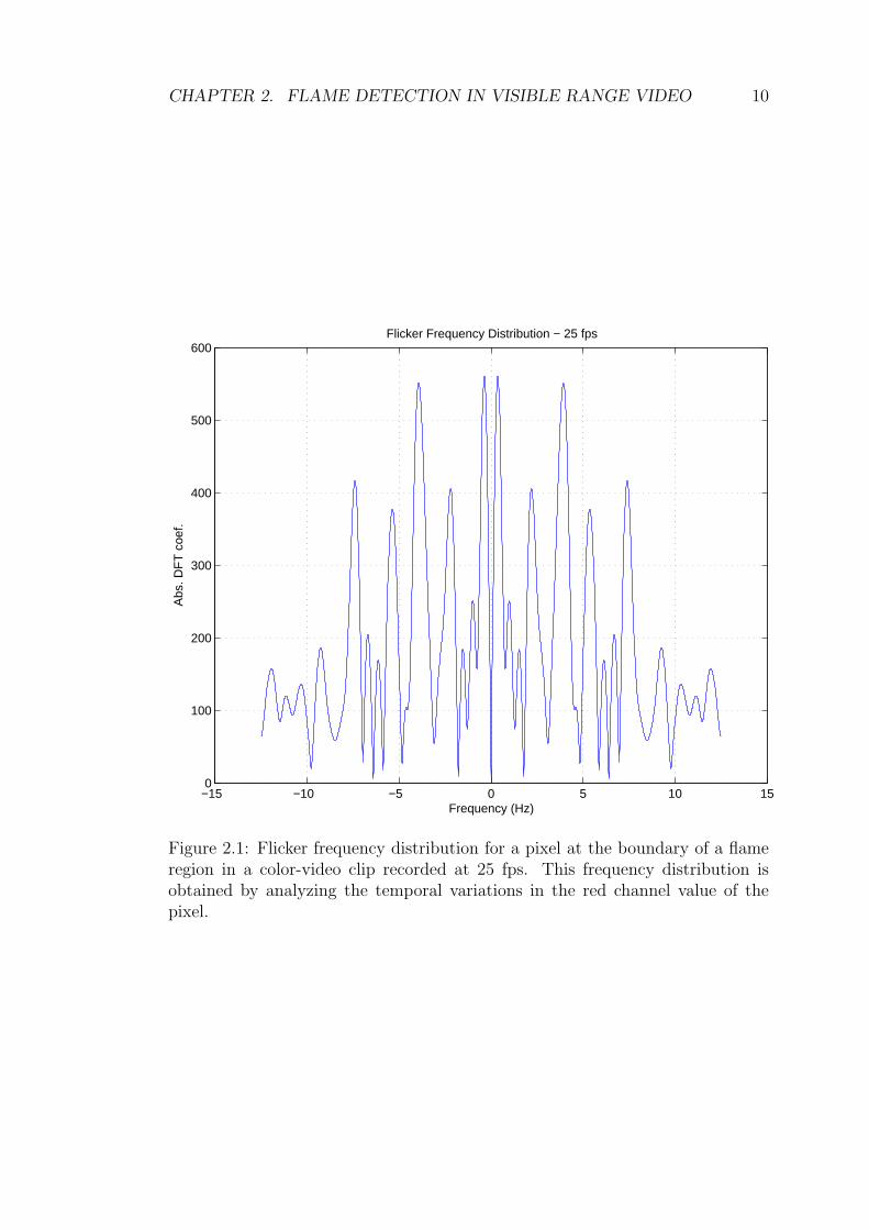
2.1 Flicker frequency distribution for a pixel at the boundary of a flame
region in a color-video clip recorded at 25 fps. This frequency
distribution is obtained by analyzing the temporal variations in
the red channel value of the pixel. . . . . . . . . . . . . . . . . . . 10
2.2 (a) A sample flame pixel process in RGB space, and (b) the spheres
centered at the means of the Gaussian distributions with radius
twice the standard deviation. . . . . . . . . . . . . . . . . . . . . 15
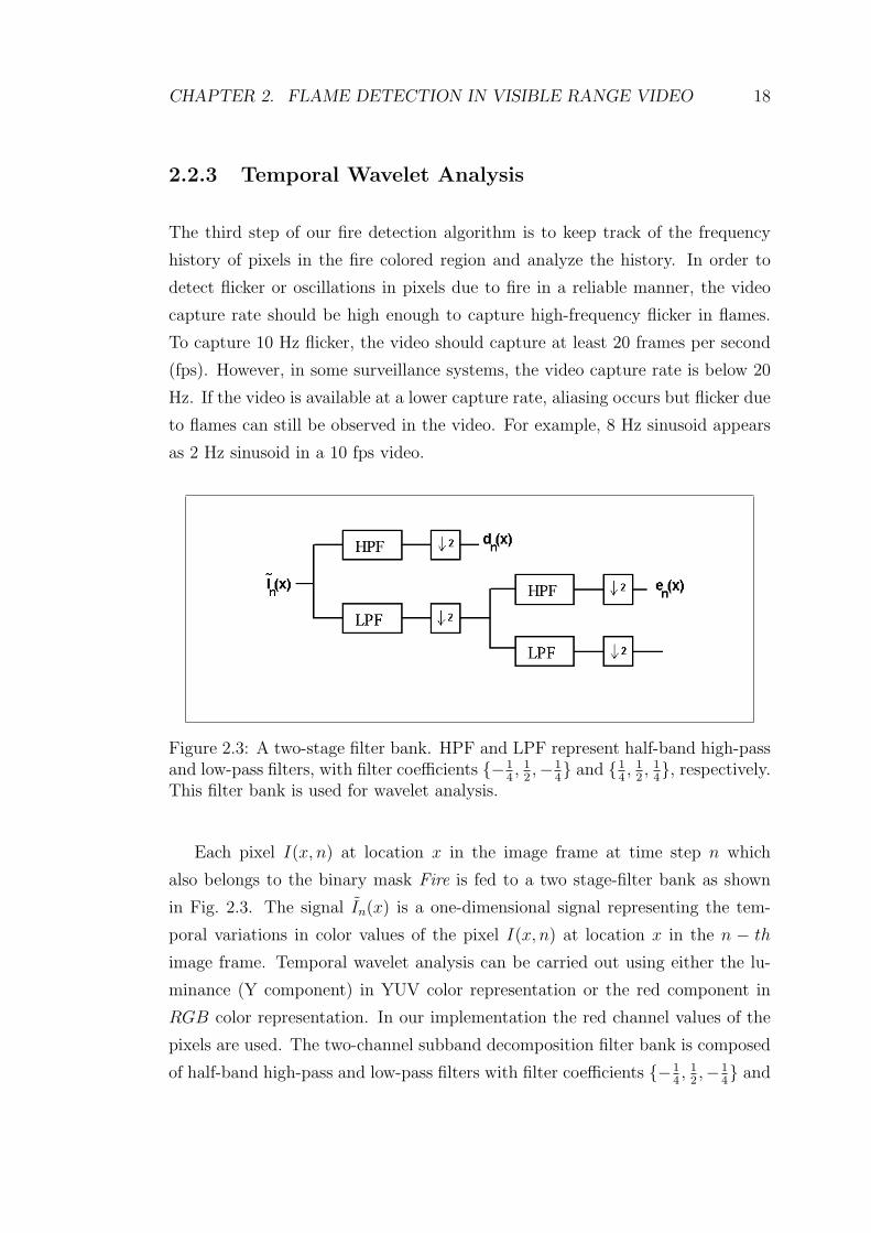
2.3 A two-stage filter bank. HPF and LPF represent half-band high-
pass and low-pass filters, with filter coefficients {−14, 1
2,−1
4} and
{14, 1
2, 1
4}, respectively. This filter bank is used for wavelet analysis. 18
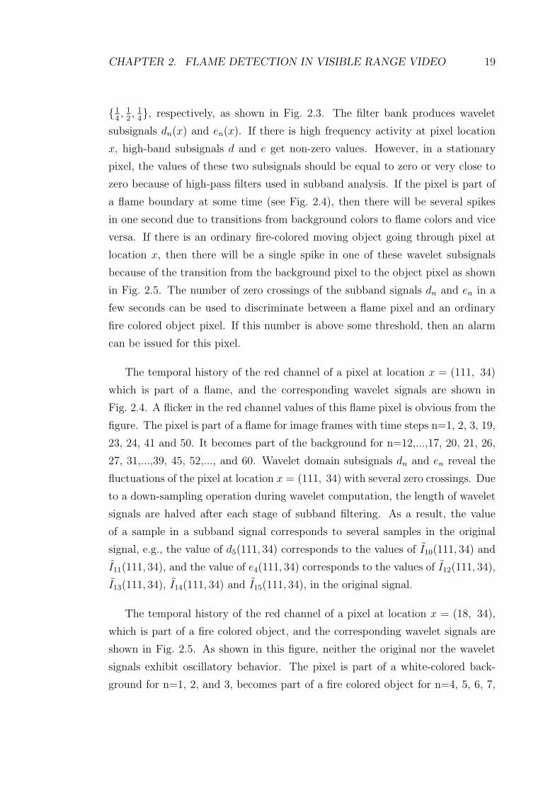
2.4 (a) Temporal variation of image pixel at location x = (111, 34),
In(x). The pixel at x = (111, 34) is part of a flame for image
frames I(x, n), n=1, 2, 3, 19, 23, 24, 41 and 50. It becomes part
of the background for n = 12,..., 17, 20, 21, 26, 27, 31,..., 39, 45,
52,..., and 60. Wavelet domain subsignals (b) dn and (c) en reveal
the fluctuations of the pixel at location x = (111, 34). . . . . . . 20
2.5 (a) Temporal history of the pixel at location x = (18, 34). It is
part of a fire-colored object for n = 4, 5, 6, 7, and 8, and it becomes
part of the background afterwards. Corresponding subsignals (b)
dn and (c) en exhibit stationary behavior for n > 8. . . . . . . . . 21
xiii

LIST OF FIGURES xiv
2.6 Three-state Markov models for a) flame and b) non-flame moving
flame-colored pixels. . . . . . . . . . . . . . . . . . . . . . . . . . 23
2.7 (a) A child with a fire-colored t-shirt, and b) the absolute sum of
spatial wavelet transform coefficients, |Ilh(k, l)|+|Ihl(k, l)|+|Ihh(k, l)|,of the region bounded by the indicated rectangle. . . . . . . . . . 26
2.8 (a) Fire, and (b) the absolute sum of spatial wavelet transform
coefficients, |Ilh(k, l)|+|Ihl(k, l)|+|Ihh(k, l)|, of the region bounded
by the indicated rectangle. . . . . . . . . . . . . . . . . . . . . . . 26
2.9 (a) With the method using color and temporal variation only
(Method-2.2) [64], false alarms are issued for the fire colored line
on the moving truck and the ground, (b) our method (Method-2.1)
does not produce any false alarms. . . . . . . . . . . . . . . . . . 28
2.10 Sample images (a) and (b) are from Movies 7 and 9, respectively.
(c) False alarms are issued for the arm of the man with the method
using color and temporal variation only (Method-2.2) [64] and (d)
on the fire-colored parking car. Our method does not give any false
alarms in such cases (see Table 2.2). . . . . . . . . . . . . . . . . . 29
2.11 Sample images (a) and (b) are from Movies 2 and 4, respectively.
Flames are successfully detected with our method (Method-2.1) in
(c) and (d). In (c), although flames are partially occluded by the
fence, a fire alarm is issued successfully. Fire pixels are painted in
bright green. . . . . . . . . . . . . . . . . . . . . . . . . . . . . . . 30
3.1 Two relatively bright moving objects in FLIR video: a) fire im-
age, and b) a man (pointed with an arrow). Moving objects are
determined by the hybrid background subtraction algorithm of [19]. 39
3.2 Equally spaced 64 contour points of the a) walking man, and b)
the fire regions shown in Fig. 3.1. . . . . . . . . . . . . . . . . . . 40

LIST OF FIGURES xv
3.3 Single-stage wavelet filter bank. The high-pass and the low-pass
filter coefficients are {−14, 1
2,−1
4} and {1
4, 1
2, 1
4}, respectively. . . . . 40
3.4 The absolute values of a) high-band (wavelet) and b) low-band co-
efficients for the fire region. . . . . . . . . . . . . . . . . . . . . . 41
3.5 The absolute a) high-band (wavelet) and b) low-band coefficients
for the walking man. . . . . . . . . . . . . . . . . . . . . . . . . . 42
3.6 Flicker frequency distributions for a) 10 fps color video, b) 25 fps
color video and c) 10 fps IR video. These frequency distributions
were obtained by analyzing the temporal variations in the red chan-
nel value of a pixel at the boundary of a flame region in color-video
clips recorded at 10 fps and 25 fps and intensity value of a pixel at
the boundary of a flame region in an IR video clip recorded at 10
fps, respectively. . . . . . . . . . . . . . . . . . . . . . . . . . . . . 44
3.7 Three-state Markov models for a) flame and b) non-flame moving
pixels. . . . . . . . . . . . . . . . . . . . . . . . . . . . . . . . . . 45
3.8 Image frames from some of the test clips. a), b) and c) Fire regions
are detected and flame boundaries are marked with arrows. d), e)
and f) No false alarms are issued for ordinary moving bright objects. 47
3.9 Image frames from some of the test clips with fire. Pixels on the
flame boundaries are successfully detected. . . . . . . . . . . . . . 48
4.1 Image frame with smoke and its single level wavelet sub-images.
Blurring in the edges is visible. The analysis is carried out in small
blocks. . . . . . . . . . . . . . . . . . . . . . . . . . . . . . . . . . 57
4.2 Single-stage wavelet filter bank. . . . . . . . . . . . . . . . . . . . 59
4.3 Three-state Markov models for smoke(left) and non-smoke moving
pixels. . . . . . . . . . . . . . . . . . . . . . . . . . . . . . . . . . 60

LIST OF FIGURES xvi
4.4 Two moving objects in video: smoke image (top), and a vehicle
(bottom). The object boundaries are determined by the back-
ground subtraction algorithm. . . . . . . . . . . . . . . . . . . . . 61
4.5 Equally spaced 64 contour points of smoke (top) and the vehicle
regions (bottom) shown in Fig.4.4. . . . . . . . . . . . . . . . . . 62
4.6 The absolute a) wavelet and b) low-band coefficients for the smoke
region. . . . . . . . . . . . . . . . . . . . . . . . . . . . . . . . . . 63
4.7 The absolute a) wavelet and b) low-band coefficients for the vehicle. 64
5.1 The circuit diagram for capturing an analog signal output from a
PIR sensor. . . . . . . . . . . . . . . . . . . . . . . . . . . . . . . 70
5.2 Flame flicker spectrum distribution. PIR signal is sampled with
50 Hz. . . . . . . . . . . . . . . . . . . . . . . . . . . . . . . . . . 71
5.3 A typical PIR sensor output sampled at 50 Hz with 8 bit quanti-
zation when there is no activity within its viewing range. . . . . . 72
5.4 PIR sensor output signals recorded at a distance of 5m for a (a)
walking person, and (b) flame. . . . . . . . . . . . . . . . . . . . . 73
5.5 Two three-state Markov models are used to represent (a) ‘fire’ and
(b) ‘non-fire’ classes, respectively. . . . . . . . . . . . . . . . . . . 75
5.6 A typical plot of the dissimilarity function D(T1,T2)x10−4. It is
multi-modal and non-differentiable. . . . . . . . . . . . . . . . . . 77
5.7 The PIR sensor is encircled. The fire is close to die out completely.
A man is also within the viewing range of the sensor. . . . . . . . 80
6.1 Snapshot of a typical wildfire smoke captured by a forest watch
tower which is 5 km away from the fire (rising smoke is marked
with an arrow). . . . . . . . . . . . . . . . . . . . . . . . . . . . . 83

LIST OF FIGURES xvii
6.2 Markov model λ1 corresponding to wildfire smoke (left) and the
Markov model λ2 of clouds (right). Transition probabilities aij
and bij are estimated off-line. . . . . . . . . . . . . . . . . . . . . 88
6.3 Orthogonal Projection: Find the vector w(n+1) on the hyperplane
y(x, n) = DT (x, n)w minimizing the distance between w(n) and
the hyperplane. . . . . . . . . . . . . . . . . . . . . . . . . . . . . 95
6.4 Geometric interpretation: Weight vectors corresponding to deci-
sion functions at each frame are updated as to satisfy the hyper-
plane equations defined by the oracle’s decision y(x, n) and the
decision vector D(x, n). Lines in the figure represent hyperplanes
in RM . . . . . . . . . . . . . . . . . . . . . . . . . . . . . . . . . . 97
6.5 The pseudo-code for the active decision fusion algorithm . . . . . 99
6.6 The pseudo-code for the universal predictor . . . . . . . . . . . . 100
6.7 The pseudo-code for the Weighted Majority Algorithm . . . . . . 101
6.8 Sequence of frames excerpted from clip V 15. Within 18 seconds
of time, cloud shadows cover forestal area which results in a false
alarm in an untrained algorithm with decision weights equal to14
depicted as a bounding box. The proposed algorithm does not
produce a false alarm in this video. . . . . . . . . . . . . . . . . . 103
6.9 The average error curves for the LMS, universal predictor, and
the WMA based adaptation algorithms in clip V 13. All of the
algorithms converge to the same average error value in this case,
however the convergence rate of the LMS algorithm is faster than
both the universal predictor and the WMA algorithm. . . . . . . . 105

List of Tables
1.1 Organization of this thesis. . . . . . . . . . . . . . . . . . . . . . . 7
2.1 The mean red, green and blue channel values and variances of ten
Gaussian distributions modeling flame color in Fig. 2.2 (b) are listed. 17
2.2 Comparison of the proposed method (Method-2.1), the method
based on color and temporal variation clues only (Method-2.2)
described in [64], and the method proposed in [17] (Method-2.3). . 33
2.3 Time performance comparison of Methods 2.1, 2.2, and 2.3 for the
movies in Table 2.2. The values are the processing times per frame
in milliseconds. . . . . . . . . . . . . . . . . . . . . . . . . . . . . 34
3.1 Detection results for some of the test clips. In the video clip V3,
flames are hindered by a wall for most of the time. . . . . . . . . . 51
3.2 Fire detection results of our method when trained with different
flame types. . . . . . . . . . . . . . . . . . . . . . . . . . . . . . . 52
3.3 Comparison of the proposed method with the modified version of
the method in [36] (CVH method) and the fire detection method
described in [87] for fire detection using a regular visible range
camera. The values for processing times per frame are in milliseconds. 52
xviii

LIST OF TABLES xix
4.1 Detection results of Method-4.1 and Method-4.2 for some live and
off-line videos. . . . . . . . . . . . . . . . . . . . . . . . . . . . . . 66
4.2 Smoke and flame detection time comparison of Method-4.1 and
Method-4.3, respectively. Smoke is an early indicator of fire. In
Movies 11 and 12, flames are not in the viewing range of the camera. 67
5.1 Results with 198 fire, 588 non-fire test sequences. The system
triggers an alarm when fire is detected within the viewing range of
the PIR sensor. . . . . . . . . . . . . . . . . . . . . . . . . . . . . 79
6.1 Frame numbers at which an alarm is issued with different methods
for wildfire smoke captured at various ranges and fps. It is assumed
that the smoke starts at frame 0. . . . . . . . . . . . . . . . . . . 104
6.2 The number of false alarms issued by different methods to video
sequences without any wildfire smoke. . . . . . . . . . . . . . . . . 105

Chapter 1
Introduction
Dynamic textures are common in many image sequences of natural scenes. Ex-
amples of dynamic textures in video include fire, smoke, clouds, volatile organic
compound (VOC) plumes in infra-red (IR) videos, trees in the wind, sea and
ocean waves, as well as traffic scenes, motion of crowds, all of which exhibit some
sort of spatio-temporal stationarity. They are also named as temporal or 3-D tex-
tures in the literature. Researchers extensively studied 2-D textures and related
problems in the fields of image processing and computer vision [32], [30]. On
the other hand, there is comparably less research conducted on dynamic texture
detection in video [18], [63], [12].
There are several approaches in the computer vision literature aiming at
recognition and synthesis of dynamic textures in video independent of their
types [71], [15], [16], [50], [29], [51], [33], [35], [89], [48], [49], [57], [79], [55],
[96], [62], [75], [28], [68], [90]. Some of these approaches model the dynamic
textures as linear dynamical systems [71], [15], [16], [50], some others use spatio-
temporal auto-regressive models [48], [79]. Other researchers in the field analyze
and model the optical flow vectors for the recognition of generic dynamic tex-
tures in video [29], [89]. In this dissertation, we do not attempt to characterize
all dynamic textures but we present smoke and fire detection methods by taking
advantage of specific properties of smoke and fire.
1
CHAPTER 1. INTRODUCTION 2
The motivation behind attacking a specific kind of recognition problem is
influenced by the notion of ‘weak’ Artificial Intelligence (AI) framework which was
first introduced by Hubert L. Dreyfus in his critique of the so called ‘generalized’
AI [25], [26]. Dreyfus presents solid philosophical and scientific arguments on why
the search for ‘generalized’ AI is futile [61]. Current content based general image
and video content understanding methods are not robust enough to be deployed
for fire detection [21], [53], [43], [54]. Instead, each specific problem should be
addressed as an individual engineering problem which has its own characteristics.
In this study, both temporal and spatial characteristics related to flames and
smoke are utilized as clues for developing solutions to the detection problem.
Another motivation for video and pyroelectric infra-red (PIR) sensor based
fire detection is that conventional point smoke and fire detectors typically detect
the presence of certain particles generated by smoke and fire by ionization or
photometry. An important weakness of point detectors is that they cannot pro-
vide quick responses in large spaces. Furthermore, conventional point detectors
cannot be utilized to detect smoldering fires in open areas.
In this thesis, novel image processing methods are proposed for the detection
of flames and smoke in open and large spaces with ranges up to 30m. Flicker
process inherent in fire is used as a clue for detection of flames and smoke in (IR)
video. A similar technique modeling flame flicker is developed for the detection
of flames using PIR sensors. Wildfire smoke appearing far away from the camera
has different spatio-temporal characteristics than nearby smoke. The algorithms
for detecting smoke due to wildfire are also proposed.
Each detection algorithm consists of several sub-algorithms each of which tries
to estimate a specific feature of the problem at hand. For example, long distance
smoke detection algorithm consists of four sub-algorithms: (i) slow moving video
object detection, (ii) smoke-colored region detection, (iii) rising video object de-
tection, (iv) shadow detection and elimination. A framework for active fusion of
decisions from these sub-algorithms is developed based on the least-mean-square
(LMS) adaptation algorithm.

CHAPTER 1. INTRODUCTION 3
No fire detection experiments were carried out using other sensing modali-
ties such as ultra-violet (UV) sensors, near infrared (NIR) or middle wave-length
infrared (MWIR) cameras, in this study. As a matter of fact, MWIR cameras
are even more expensive than LWIR cameras. Therefore, deploying MWIR cam-
eras for fire monitoring turns out to be an unfeasible option for most practical
applications.
There are built-in microphones in most of the off-the-shelf surveillance cam-
eras. Audio data captured from these microphones can be also analyzed along
with the video data in fire monitoring applications. One can develop fire detec-
tion methods exploiting data coming from several sensing modalities similar to
methods described in [31], [85], [88], [24].
1.1 Contribution of this Thesis
The major contributions of this thesis can be divided into two main categories.
1.1.1 Markov Models Using Wavelet Domain Features for
Short Range Flame and Smoke Detection
A common feature of all the algorithms developed in this thesis is the use of
wavelets and Markov models. In the proposed approach wavelets or sub-band
analysis are used in dynamic texture modeling. This leads to computationally
efficient algorithms for texture feature analysis, because computing wavelet coef-
ficients is an Order-(N) type operation. In addition, we do not try to determine
edges or corners in a given scene. We simply monitor the decay or increase in
wavelet coefficients’ sub-band energies both temporally and spatially.
Another important feature of the proposed smoke and fire detection methods is
the use of Markov models to characterize temporal motion in the scene. Turbulent
fire behavior is a random phenomenon which can be conveniently modeled in a

CHAPTER 1. INTRODUCTION 4
Markovian setting.
In the following sub-sections, the general overview of the proposed algorithms
are developed. In all methods, it is assumed that a stationary camera monitors
the scene.
1.1.1.1 Flame Detection in Visible Range Video
Novel real-time signal processing techniques are developed to detect flames by
processing the video data generated by a visible range camera. In addition to
motion and color clues used by [64], flame flicker is detected by analyzing the
video in wavelet domain. Turbulent behavior in flame boundaries is detected by
performing temporal wavelet transform. Wavelet coefficients are used as feature
parameters in Hidden Markov Models (HMMs). A Markov model is trained with
flames and another is trained with ordinary activity of human beings and other
flame colored moving objects. Flame flicker process is also detected by using an
HMM. Markov models representing the flame and flame colored ordinary moving
objects are used to distinguish flame flicker process from motion of flame colored
moving objects.
Other clues used in the fire detection algorithm include irregularity of the
boundary of the fire colored region and the growth of such regions in time. All
these clues are combined to reach a final decision. The main contribution of the
proposed video based fire detection method is the analysis of the flame flicker and
integration of this clue as a fundamental step in the detection process.
1.1.1.2 Flame Detection in IR Video
A novel method to detect flames in videos captured with Long-Wavelength Infra-
Red (LWIR) cameras is proposed, as well. These cameras cover 8-12µm range in
the electromagnetic spectrum. Image regions containing flames appear as bright
regions in IR video. In addition to motion and brightness clues, flame flicker
process is also detected by using an HMM describing the temporal behavior as in

CHAPTER 1. INTRODUCTION 5
the previous algorithm. IR image frames are also analyzed spatially. Boundary
of flames are represented in wavelet domain and high frequency nature of the
boundaries of fire regions is also used as a clue to model the flame flicker.
All of the temporal and spatial clues extracted from the IR video are combined
to reach a final decision. False alarms due to ordinary bright moving objects are
greatly reduced because of the HMM based flicker modeling and wavelet domain
boundary modeling. The contribution of this work is the introduction of a novel
sub-band energy based feature for the analysis of flame region boundaries.
1.1.1.3 Short-range Smoke Detection in Video
Smoldering smoke appears first, even before flames, in most fires. Contrary to
the common belief, smoke cannot be visualized in LWIR (8-12µm range) video.
A novel method to detect smoke in video is developed.
The smoke is semi-transparent at the early stages of a fire. Therefore edges
present in image frames start loosing their sharpness and this leads to a decrease
in the high frequency content of the image. The background of the scene is
estimated and decrease of high frequency energy of the scene is monitored using
the spatial wavelet transforms of the current and the background images.
Edges of the scene produce local extrema in the wavelet domain and a decrease
in the energy content of these edges is an important indicator of smoke in the
viewing range of the camera. Moreover, scene becomes grayish when there is
smoke and this leads to a decrease in chrominance values of pixels. Random
behavior in smoke boundaries is also analyzed using an HMM mimicking the
temporal behavior of the smoke. In addition, boundaries of smoke regions are
represented in wavelet domain and high frequency nature of the boundaries of
smoke regions is also used as a clue to model the smoke flicker. All these clues
are combined to reach a final decision.
Monitoring the decrease in the sub-band image energies corresponding to
smoke regions in video constitutes the main contribution of this work.

CHAPTER 1. INTRODUCTION 6
1.1.1.4 Flame Detection Using PIR sensors
A flame detection system based on a pyroelectric (or passive) infrared (PIR) sen-
sor is developed. This algorithm is similar to the video flame detection algorithm.
The PIR sensor can be considered as a single pixel camera. Therefore an algo-
rithm for flame detection for PIR sensors can be developed by simply removing
the spatial analysis steps of the video flame detection method.
The flame detection system can be used for fire detection in large rooms. The
flame flicker process of an uncontrolled fire and ordinary activity of human beings
and other objects are modeled using a set of Hidden Markov Models (HMM),
which are trained using the wavelet transform of the PIR sensor signal. Whenever
there is an activity within the viewing range of the PIR sensor system, the sensor
signal is analyzed in the wavelet domain and the wavelet signals are fed to a set
of HMMs. A fire or no fire decision is made according to the HMM producing
the highest probability.
1.1.2 Wildfire Detection with Active Learning Based on
the LMS Algorithm
Wildfire smoke has different spatio-temporal characteristics than nearby smoke,
because wildfire usually starts far away from forest look-out towers. The
main wildfire (long-range smoke) detection algorithm is composed of four sub-
algorithms detecting (i) slow moving objects, (ii) smoke-colored regions, (iii) ris-
ing regions, and (iv) shadows. Each sub-algorithm yields its own decision as
a zero-mean real number, representing the confidence level of that particular
sub-algorithm. Confidence values are linearly combined with weights determined
according to a novel active fusion method based on the least-mean-square (LMS)
algorithm which is a widely used technique in adaptive filtering. Weights are up-
dated on-line using the LMS method in the training (learning) stage. The error
function of the LMS based training process is defined as the difference between
the weighted sum of decision values and the decision of an oracle, who is the

CHAPTER 1. INTRODUCTION 7
security guard of the forest look-out tower.
The contribution of this work is twofold; a novel video based wildfire detection
method and a novel active learning framework based on the LMS algorithm. The
proposed adaptive fusion strategy can be used in many supervised learning based
computer vision applications comprising of several sub-algorithms.
1.2 Thesis Outline
The outline of the thesis is as follows. In Chapters 2 and 3, wavelet and HMM
based methods for flame detection in visible and IR range video are presented,
respectively. The short-range smoke detection algorithm is presented in Chapter
4. Detection of flames using PIR sensors is discussed in Chapter 5. In Chapter
6, wildfire (long-range smoke) detection with active learning based on the LMS
algorithm is described. Finally Chapter 7 concludes this thesis by providing an
overall summary of the results. Possible research areas in the future are provided,
as well.
The organization of this thesis is presented in Table 1.1. Note that, smoke
detection methods could only be developed for visible range cameras due to the
fact that smoke cannot be visualized with PIR sensors and LWIR cameras.
Table 1.1: Organization of this thesis.
Sensor type Flame Short-range (< 30m) Long distance (> 100m)Smoke Smoke
Visible Range Camera Chapter 2 Chapter 4 Chapter 6LWIR Camera Chapter 3 N/A N/A
PIR Sensor Chapter 5 N/A N/A
Chapter 2
Flame Detection in Visible
Range Video
In this chapter, the previous work in the literature on video based fire detection is
summarized, first. Then, the proposed wavelet analysis and Markov model based
detection method characterizing the flame flicker process is described. Markov
model based approach reduces the number of false alarms issued to ordinary
fire-colored moving objects as compared to the methods using only motion and
color clues. Experimental results show that the proposed method is successful in
detecting flames.
2.1 Related Work
Video based fire detection systems can be useful for detecting fire in covered ar-
eas including auditoriums, tunnels, atriums, etc., in which conventional chemical
fire sensors cannot provide quick responses to fire. Furthermore, closed circuit
television (CCTV) surveillance systems are currently installed in various public
places monitoring indoors and outdoors. Such systems may gain an early fire de-
tection capability with the use of a fire detection software processing the outputs
of CCTV cameras in real time.
8

CHAPTER 2. FLAME DETECTION IN VISIBLE RANGE VIDEO 9
There are several video-based fire and flame detection algorithms in the lit-
erature [64], [17], [48], [78], [38], [81], [80], [94]. These methods make use of
various visual signatures including color, motion and geometry of fire regions.
Healey et al. [38] use only color clues for flame detection. Phillips et al. [64]
use pixel colors and their temporal variations. Chen et al. [17] utilize a change
detection scheme to detect flicker in fire regions. In [78], Fast Fourier Trans-
forms (FFT) of temporal object boundary pixels are computed to detect peaks
in Fourier domain, because it is claimed that turbulent flames flicker with a char-
acteristic flicker frequency of around 10 Hz independent of the burning material
and the burner in a mechanical engineering paper [1], [14]. We observe that flame
flicker process is a wide-band activity below 12.5 Hz in frequency domain for a
pixel at the boundary of a flame region in a color-video clip recorded at 25 fps
(cf. Fig. 2.1). Liu and Ahuja [48] also represent the shapes of fire regions in
Fourier domain. However, an important weakness of Fourier domain methods is
that flame flicker is not purely sinusoidal but it’s random in nature. Therefore,
there may not be any peaks in FFT plots of fire regions. In addition, Fourier
Transform does not have any time information. Therefore, Short-Time Fourier
Transform (STFT) can be used requiring a temporal analysis window. In this
case, temporal window size becomes an important parameter for detection. If
the window size is too long, one may not observe peakiness in the FFT data. If
it is too short, one may completely miss cycles and therefore no peaks can be
observed in the Fourier domain.
Our method not only detects fire and flame colored moving regions in video but
also analyzes the motion of such regions in wavelet domain for flicker estimation.
The appearance of an object whose contours, chrominance or luminosity values
oscillate at a frequency higher than 0.5 Hz in video is an important sign of the
possible presence of flames in the monitored area [78].
High-frequency analysis of moving pixels is carried out in wavelet domain in
our work. There is an analogy between the proposed wavelet domain motion anal-
ysis and the temporal templates of [21] and the motion recurrence images of [43],
which are ad hoc tools used by computer scientists to analyze dancing people
and periodically moving objects and body parts. However, temporal templates
CHAPTER 2. FLAME DETECTION IN VISIBLE RANGE VIDEO 10
−15 −10 −5 0 5 10 150
100
200
300
400
500
600
Frequency (Hz)
Abs
. DF
T c
oef.
Flicker Frequency Distribution − 25 fps
Figure 2.1: Flicker frequency distribution for a pixel at the boundary of a flameregion in a color-video clip recorded at 25 fps. This frequency distribution isobtained by analyzing the temporal variations in the red channel value of thepixel.

CHAPTER 2. FLAME DETECTION IN VISIBLE RANGE VIDEO 11
and motion recurrence images do not provide a quantitative frequency domain
measure. On the other hand, wavelet transform is a time-frequency analysis tool
providing both partial frequency and time information about the signal. One
can examine an entire frequency band in the wavelet domain without completely
loosing the time information [10], [52]. Since the wavelet transform is computed
using a subband decomposition filter bank, it does not require any batch pro-
cessing. It is ideally suited to determine an increase in high-frequency activity in
fire and flame colored moving objects by detecting zero crossings of the wavelet
transform coefficients.
In practice, flame flicker process is time-varying and it is far from being pe-
riodic. This stochastic behavior in flicker frequency is especially valid for uncon-
trolled fires. Therefore, a random model based modeling of flame flicker process
produces more robust performance compared to frequency domain based methods
which try to detect peaks around 10 Hz in the Fourier domain. In [84], fire and
flame flicker is modeled by using HMMs trained with pixel domain features in
video. In this thesis, temporal wavelet coefficients are used as feature parameters
in Markov models.
Turbulent high-frequency behaviors exist not only on the boundary but also
inside a fire region. Another novelty of the proposed method is the analysis of
the spatial variations inside fire and flame colored regions. The method described
in [78] does not take advantage of such color variations. Spatial wavelet analysis
makes it possible to detect high-frequency behavior inside fire regions. Variation
in energy of wavelet coefficients is an indicator of activity within the region. On
the other hand, a fire colored moving object will not exhibit any change in values
of wavelet coefficients because there will not be any variation in fire colored pixel
values. Spatial wavelet coefficients are also used in Markov models to characterize
the turbulent behavior within fire regions.

CHAPTER 2. FLAME DETECTION IN VISIBLE RANGE VIDEO 12
2.2 Steps of Video Flame Detection Algorithm
The proposed video-based fire detection algorithm consists of four sub-algorithms:
(i) moving pixels or regions in the current frame of a video are determined, (ii)
colors of moving pixels are checked to see if they match to pre-specified fire colors.
Afterwards, wavelet analysis in (iii) temporal and (iv) spatial domains are carried
out to determine high-frequency activity within these moving regions. Each step
of the proposed algorithm is explained in detail in the sequel.
2.2.1 Moving Region Detection
Background subtraction is commonly used for segmenting out moving objects
in a scene for surveillance applications. There are several methods in the lit-
erature [19], [3], [77]. The background estimation algorithm described in [19]
uses a simple IIR filter applied to each pixel independently to update the back-
ground and use adaptively updated thresholds to classify pixels into foreground
and background.
Stationary pixels in the video are the pixels of the background scene because
the background can be defined as temporally stationary part of the video.If the
scene is observed for some time, then pixels forming the entire background scene
can be estimated because moving regions and objects occupy only some parts
of the scene in a typical image of a video. A simple approach to estimate the
background is to average the observed image frames of the video. Since moving
objects and regions occupy only a part of the image, they conceal a part of the
background scene and their effect is canceled over time by averaging. Our main
concern is real-time performance of the system. In Video Surveillance and Moni-
toring (VSAM) Project at Carnegie Mellon University [19] a recursive background
estimation method was developed from the actual image data using `1-norm based
calculations.
Let I(x, n) represent the intensity value of the pixel at location x in the n− th
video frame I. Estimated background intensity value, B(x, n + 1), at the same

CHAPTER 2. FLAME DETECTION IN VISIBLE RANGE VIDEO 13
pixel position is calculated as follows:
B(x, n + 1) =
{aB(x, n) + (1− a)I(x, n) if x is stationary
B(x, n) if x is a moving pixel(2.1)
where B(x, n) is the previous estimate of the background intensity value at the
same pixel position. The update parameter a is a positive real number close to
one. Initially, B(x, 0) is set to the first image frame I(x, 0). A pixel positioned
at x is assumed to be moving if:
|I(x, n)− I(x, n− 1)| > T (x, n) (2.2)
where I(x, n−1) is the intensity value of the pixel at location x in the (n−1)−th
video frame I and T (x, n) is a recursively updated threshold at each frame n,
describing a statistically significant intensity change at pixel position x:
T (x, n + 1) =
{aT (x, n) + (1− a)(c|I(x, n)−B(x, n)|) if x is stationary
T (x, n) if x is a moving pixel
(2.3)
where c is a real number greater than one and the update parameter a is a positive
number close to one. Initial threshold values are set to a pre-determined non-zero
value.
Both the background image B(x, n) and the threshold image T (x, n) are sta-
tistical blue prints of the pixel intensities observed from the sequence of images
{I(x, k)} for k < n. The background image B(x, n) is analogous to a local tem-
poral average of intensity values, and T (x, n) is analogous to c times the local
temporal standard deviation of intensity in `1-norm [19].
As it can be seen from Eq. 2.3, the higher the parameter c, higher the threshold
or lower the sensitivity of detection scheme. It is assumed that regions signifi-
cantly different from the background are moving regions. Estimated background
image is subtracted from the current image to detect moving regions which cor-
responds to the set of pixels satisfying:
|I(x, n)−B(x, n)| > T (x, n) (2.4)
are determined. These pixels are grouped into connected regions (blobs) and
labeled by using a two-level connected component labeling algorithm [40]. The
CHAPTER 2. FLAME DETECTION IN VISIBLE RANGE VIDEO 14
output of the first step of the algorithm is a binary pixel map Blobs(x,n) that
indicates whether or not the pixel at location x in n− th frame is moving.
Other more sophisticated methods, including the ones developed by
Bagci et al. [3] and Stauffer and Grimson [77], can also be used for moving
pixel estimation. In our application, accurate detection of moving regions is not
as critical as in other object tracking and estimation problems; we are mainly
concerned with real-time detection of moving regions as an initial step in the fire
and flame detection system. We choose to implement the method suggested by
Collins et al. [19], because of its computational efficiency.
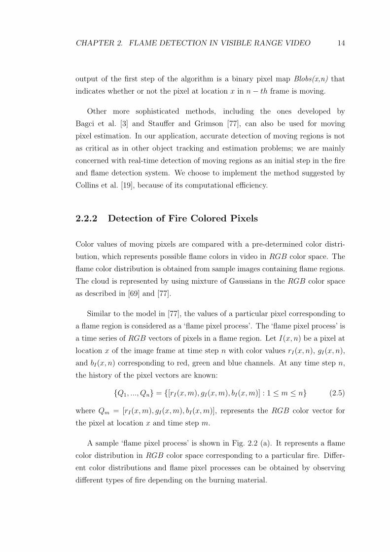
2.2.2 Detection of Fire Colored Pixels
Color values of moving pixels are compared with a pre-determined color distri-
bution, which represents possible flame colors in video in RGB color space. The
flame color distribution is obtained from sample images containing flame regions.
The cloud is represented by using mixture of Gaussians in the RGB color space
as described in [69] and [77].
Similar to the model in [77], the values of a particular pixel corresponding to
a flame region is considered as a ‘flame pixel process’. The ‘flame pixel process’ is
a time series of RGB vectors of pixels in a flame region. Let I(x, n) be a pixel at
location x of the image frame at time step n with color values rI(x, n), gI(x, n),
and bI(x, n) corresponding to red, green and blue channels. At any time step n,
the history of the pixel vectors are known:
{Q1, ..., Qn} = {[rI(x,m), gI(x, m), bI(x, m)] : 1 ≤ m ≤ n} (2.5)
where Qm = [rI(x,m), gI(x,m), bI(x,m)], represents the RGB color vector for
the pixel at location x and time step m.
A sample ‘flame pixel process’ is shown in Fig. 2.2 (a). It represents a flame
color distribution in RGB color space corresponding to a particular fire. Differ-
ent color distributions and flame pixel processes can be obtained by observing
different types of fire depending on the burning material.

CHAPTER 2. FLAME DETECTION IN VISIBLE RANGE VIDEO 15
(a)
(b)
Figure 2.2: (a) A sample flame pixel process in RGB space, and (b) the spherescentered at the means of the Gaussian distributions with radius twice the standarddeviation.

CHAPTER 2. FLAME DETECTION IN VISIBLE RANGE VIDEO 16
A Gaussian mixture model with D Gaussian distributions is used to model
the past observations {Q1, ..., Qn}
P (Qn) =D∑
d=1
η(Qn|µd,n, Σd,n) (2.6)
where D is the number of distributions, µd,n is the mean value of the d-th Gaussian
in the mixture at time step n, Σd,n is the covariance matrix of the d-th Gaussian
in the mixture at time step n, and η is a Gaussian probability density function
η(Q|µ, Σ) =1
(2π)n2 |Σ| 12
e−12(Q−µ)T Σ−1(Q−µ) (2.7)
In our implementation, we model the flame color distribution with D = 10 Gaus-
sians. In order to lower computational cost, red, blue and green channel values
of pixels are assumed to be independent and have the same variance [77]. This
assumption results in a covariance matrix of the form:
Σd,n = σ2dI (2.8)
where I is the 3-by-3 identity matrix.
In the training phase, each observation vector, Qn, is checked with the existing
D distributions for a possible match. In the preferred embodiment, a match is
defined as an RGB vector within 2 standard deviations of a distribution. If
none of the D distributions match the current observation vector, Qn, the least
probable distribution is replaced with a distribution with the current observation
vector as its mean value and a high initial variance.
The mean and the standard deviation values of the un-matched distributions
are kept the same. However, both the mean and the variance of the matching
distribution with the current observation vector, Qn, are updated. Let the match-
ing distribution with the current observation vector, Qn, be the d-th Gaussian
with mean µd,n and standard deviation σd,n. The mean, µd,n, of the matching
distribution is updated as:
µd,n = (1− c)µd,n−1 + cQn (2.9)
and the variance, σ2d,n, is updated as:
σ2d,n = (1− c)σ2
d,n−1 + c(Qn − µd,n)T (Qn − µd,n) (2.10)

CHAPTER 2. FLAME DETECTION IN VISIBLE RANGE VIDEO 17
Table 2.1: The mean red, green and blue channel values and variances of tenGaussian distributions modeling flame color in Fig. 2.2 (b) are listed.
Distribution Red Green Blue Variance1 121.16 76.87 43.98 101.162 169.08 84.14 35.20 102.773 177.00 104.00 62.00 100.004 230.42 113.78 43.71 107.225 254.47 214.66 83.08 100.116 254.97 159.06 151.00 100.087 254.98 140.98 141.93 100.398 254.99 146.95 102.99 99.579 255.00 174.08 175.01 101.0110 255.00 217.96 176.07 100.78
where
c = η(Qn|µd,n, Σd,n) (2.11)
A Gaussian mixture model with ten Gaussian distributions is presented in
Fig. 2.2 (b). In this figure, spheres centered at the mean values of Gaussians
have radii twice the corresponding standard deviations. The mean red, green
and blue values and variances of Gaussian distributions in Fig. 2.2 (b) are listed
in Table 2.1.
Once flame pixel process is modeled and fixed in the training phase, the
RGB color vector of a pixel is checked whether the pixel lies within two standard
deviations of the centers of the Gaussians to determine its nature. In other words,
if a given pixel color value is inside one of the spheres shown in Fig. 2.2 (b), then
it is assumed to be a fire colored pixel. We set a binary mask, called FireColored,
which returns whether a given pixel is fire colored or not. The intersection of this
mask with Blobs formed in the first step is fed into the next step as a new binary
mask called Fire.
CHAPTER 2. FLAME DETECTION IN VISIBLE RANGE VIDEO 18
2.2.3 Temporal Wavelet Analysis
The third step of our fire detection algorithm is to keep track of the frequency
history of pixels in the fire colored region and analyze the history. In order to
detect flicker or oscillations in pixels due to fire in a reliable manner, the video
capture rate should be high enough to capture high-frequency flicker in flames.
To capture 10 Hz flicker, the video should capture at least 20 frames per second
(fps). However, in some surveillance systems, the video capture rate is below 20
Hz. If the video is available at a lower capture rate, aliasing occurs but flicker due
to flames can still be observed in the video. For example, 8 Hz sinusoid appears
as 2 Hz sinusoid in a 10 fps video.
Figure 2.3: A two-stage filter bank. HPF and LPF represent half-band high-passand low-pass filters, with filter coefficients {−1
4, 1
2,−1
4} and {1
4, 1
2, 1
4}, respectively.
This filter bank is used for wavelet analysis.
Each pixel I(x, n) at location x in the image frame at time step n which
also belongs to the binary mask Fire is fed to a two stage-filter bank as shown
in Fig. 2.3. The signal In(x) is a one-dimensional signal representing the tem-
poral variations in color values of the pixel I(x, n) at location x in the n − th
image frame. Temporal wavelet analysis can be carried out using either the lu-
minance (Y component) in YUV color representation or the red component in
RGB color representation. In our implementation the red channel values of the
pixels are used. The two-channel subband decomposition filter bank is composed
of half-band high-pass and low-pass filters with filter coefficients {−14, 1
2,−1
4} and
CHAPTER 2. FLAME DETECTION IN VISIBLE RANGE VIDEO 19
{14, 1
2, 1
4}, respectively, as shown in Fig. 2.3. The filter bank produces wavelet
subsignals dn(x) and en(x). If there is high frequency activity at pixel location
x, high-band subsignals d and e get non-zero values. However, in a stationary
pixel, the values of these two subsignals should be equal to zero or very close to
zero because of high-pass filters used in subband analysis. If the pixel is part of
a flame boundary at some time (see Fig. 2.4), then there will be several spikes
in one second due to transitions from background colors to flame colors and vice
versa. If there is an ordinary fire-colored moving object going through pixel at
location x, then there will be a single spike in one of these wavelet subsignals
because of the transition from the background pixel to the object pixel as shown
in Fig. 2.5. The number of zero crossings of the subband signals dn and en in a
few seconds can be used to discriminate between a flame pixel and an ordinary
fire colored object pixel. If this number is above some threshold, then an alarm
can be issued for this pixel.
The temporal history of the red channel of a pixel at location x = (111, 34)
which is part of a flame, and the corresponding wavelet signals are shown in
Fig. 2.4. A flicker in the red channel values of this flame pixel is obvious from the
figure. The pixel is part of a flame for image frames with time steps n=1, 2, 3, 19,
23, 24, 41 and 50. It becomes part of the background for n=12,...,17, 20, 21, 26,
27, 31,...,39, 45, 52,..., and 60. Wavelet domain subsignals dn and en reveal the
fluctuations of the pixel at location x = (111, 34) with several zero crossings. Due
to a down-sampling operation during wavelet computation, the length of wavelet
signals are halved after each stage of subband filtering. As a result, the value
of a sample in a subband signal corresponds to several samples in the original
signal, e.g., the value of d5(111, 34) corresponds to the values of I10(111, 34) and
I11(111, 34), and the value of e4(111, 34) corresponds to the values of I12(111, 34),
I13(111, 34), I14(111, 34) and I15(111, 34), in the original signal.
The temporal history of the red channel of a pixel at location x = (18, 34),
which is part of a fire colored object, and the corresponding wavelet signals are
shown in Fig. 2.5. As shown in this figure, neither the original nor the wavelet
signals exhibit oscillatory behavior. The pixel is part of a white-colored back-
ground for n=1, 2, and 3, becomes part of a fire colored object for n=4, 5, 6, 7,

CHAPTER 2. FLAME DETECTION IN VISIBLE RANGE VIDEO 20
Figure 2.4: (a) Temporal variation of image pixel at location x = (111, 34), In(x).The pixel at x = (111, 34) is part of a flame for image frames I(x, n), n=1, 2, 3,19, 23, 24, 41 and 50. It becomes part of the background for n = 12,..., 17, 20,21, 26, 27, 31,..., 39, 45, 52,..., and 60. Wavelet domain subsignals (b) dn and (c)en reveal the fluctuations of the pixel at location x = (111, 34).

CHAPTER 2. FLAME DETECTION IN VISIBLE RANGE VIDEO 21
Figure 2.5: (a) Temporal history of the pixel at location x = (18, 34). It ispart of a fire-colored object for n = 4, 5, 6, 7, and 8, and it becomes part ofthe background afterwards. Corresponding subsignals (b) dn and (c) en exhibitstationary behavior for n > 8.

CHAPTER 2. FLAME DETECTION IN VISIBLE RANGE VIDEO 22
and 8, then it becomes part of the background again for n > 8. Corresponding
wavelet signals dn and en do not exhibit oscillatory behavior as shown in Fig. 2.5.
Small variations due to noise around zero after the 10− th frame are ignored by
setting up a threshold.
The number of wavelet stages needed for used in flame flicker analysis is
determined by the video capture rate. In the first stage of dyadic wavelet de-
composition, the low-band subsignal and the high-band wavelet subsignal dn(x)
of the signal In(x) are obtained. The subsignal dn(x) contains [2.5 Hz, 5 Hz]
frequency band information of the original signal In(x) in 10 Hz video frame
rate. In the second stage the low-band subsignal is processed once again using a
dyadic filter bank, and the wavelet subsignal en(x) covering the frequency band
[1.25 Hz, 2.5 Hz] is obtained. Thus by monitoring wavelet subsignals en(x) and
dn(x), one can detect fluctuations between 1.25 to 5 Hz in the pixel at location x.
Flame flicker can be detected in low-rate image sequences obtained with a rate
of less than 20 Hz as well in spite of the aliasing phenomenon. To capture 10 Hz
flicker, the video should capture at least 20 frames per second (fps). However, in
some surveillance systems, the video capture rate is below 20 Hz. If the video is
available at a lower capture rate, aliasing occurs but flicker due to flames can still
be observed in the video. For example, 8 Hz sinusoid appears as 2 Hz sinusoid in a
10 fps video [87]. Aliased version of flame flicker signal is also a wide-band signal
in discrete-time Fourier Transform domain. This characteristic flicker behavior is
very well suited to be modeled as a random Markov model which is extensively
used in speech recognition systems and recently these models have been used in
computer vision applications [6].
Three-state Markov models are trained off-line for both flame and non-flame
pixels to represent the temporal behavior (cf. Fig.4.3). These models are trained
by using first-level wavelet coefficients dn(x) corresponding to the intensity values
In(x) of the flame-colored moving pixel at location x as the feature signal. A
single-level decomposition of the intensity variation signal In(x) is sufficient to
characterize the turbulent nature of flame flicker. One may use higher-order
wavelet coefficients such as, en(x), for flicker characterization, as well. However,

CHAPTER 2. FLAME DETECTION IN VISIBLE RANGE VIDEO 23
this may incur additional delays in detection.
Figure 2.6: Three-state Markov models for a) flame and b) non-flame movingflame-colored pixels.
Wavelet signals can easily reveal the random characteristic of a given signal
which is an intrinsic nature of flame pixels. That is why the use of wavelets
instead of actual pixel values lead to more robust detection of flames in video.
Since, wavelet signals are high-pass filtered signals, slow variations in the original
signal lead to zero-valued wavelet coefficients. Hence it is easier to set thresholds
in the wavelet domain to distinguish slow varying signals from rapidly changing
signals. Non-negative thresholds T1 < T2 are introduced in wavelet domain to
define the three states of the Hidden Markov Models for flame and non-flame
moving bright objects. For the pixels of regular hot objects like walking people,
engine of a moving car, etc., no rapid changes take place in the pixel values.
Therefore, the temporal wavelet coefficients ideally should be zero but due to
thermal noise of the camera the wavelet coefficients wiggle around zero. The
lower threshold T1 basically determines a given wavelet coefficient being close to
zero. The second threshold T2 indicates that the wavelet coefficient is significantly
higher than zero. When the wavelet coefficients fluctuate between values above
the higher threshold T2 and below the lower threshold T1 in a frequent manner
this indicates the existence of flames in the viewing range of the camera.

CHAPTER 2. FLAME DETECTION IN VISIBLE RANGE VIDEO 24
The states of HMMs are defined as follows: at time n, if |w(n)| < T1, the
state is in S1; if T1 < |w(n)| < T2, the state is S2; else if |w(n)| > T2, the
state S3 is attained. For the pixels of regular flame-colored moving objects, like
walking people in red shirts, no rapid changes take place in the pixel values.
Therefore, the temporal wavelet coefficients ideally should be zero but due to
thermal noise of the camera the wavelet coefficients wiggle around zero. The
lower threshold T1 basically determines a given wavelet coefficient being close to
zero. The state defined for the wavelet coefficients below T1 is S1. The second
threshold T2 indicates that the wavelet coefficient is significantly higher than zero.
The state defined for the wavelet coefficients above this second threshold T2 is
S3. The values between T1 and T2 define S2. The state S2 provides hysteresis
and it prevents sudden transitions from S1 to S3 or vice versa. When the wavelet
coefficients fluctuate between values above the higher threshold T2 and below the
lower threshold T1 in a frequent manner this indicates the existence of flames in
the viewing range of the camera.
In flame pixels, the transition probabilities a’s should be high and close to each
other due to random nature of uncontrolled fire. On the other hand, transition
probabilities should be small in constant temperature moving bodies because
there is no change or little change in pixel values. Hence we expect a higher
probability for b00 than any other b value in the non-flame moving pixels model
(cf. Fig.4.3), which corresponds to higher probability of being in S1. The state
S2 provides hysteresis and it prevents sudden transitions from S1 to S3 or vice
versa.
The transition probabilities between states for a pixel are estimated during a
pre-determined period of time around flame boundaries. In this way, the model
not only learns the way flame boundaries flicker during a period of time, but also
it tailors its parameters to mimic the spatial characteristics of flame regions. The
way the model is trained as such, drastically reduces the false alarm rates.
During the recognition phase, the HMM based analysis is carried out in pixels
near the contour boundaries of flame-colored moving regions. The state sequence
of length 20 image frames is determined for these candidate pixels and fed to

CHAPTER 2. FLAME DETECTION IN VISIBLE RANGE VIDEO 25
the flame and non-flame pixel models. The model yielding higher probability is
determined as the result of the analysis for each of the candidate pixel. A pixel
is called as a flame or a non-flame pixel according to the result of this analysis.
A fire mask composing of flame pixels is formed as the output of the method.
The probability of a Markov model producing a given sequence of wavelet coef-
ficients is determined by the sequence of state transition probabilities. Therefore,
the flame decision process is insensitive to the choice of thresholds T1 and T2,
which basically determine if a given wavelet coefficient is close to zero or not.
Still, thresholds can be determined using a k-means type algorithm, as well.
2.2.4 Spatial Wavelet Analysis
The fourth step of our fire detection algorithm is the spatial wavelet analysis of
moving regions containing Fire mask pixels to capture color variations in pixel
values. In an ordinary fire-colored object there will be little spatial variations in
the moving region as shown in Fig. 2.7 (a). On the other hand, there will be
significant spatial variations in a fire region as shown in Fig. 2.8 (a). The spatial
wavelet analysis of a rectangular frame containing the pixels of fire-colored moving
regions is performed. The images in Figs. 2.7 (b) and 2.8 (b) are obtained after a
single stage two-dimensional wavelet transform that is implemented in a separable
manner using the same filters explained in Subsection 2.2.3. Absolute values of
low-high, high-low and high-high wavelet subimages are added to obtain these
images. A decision parameter v4 is defined for this step, according to the energy
of the wavelet subimages:
v4 =1
M ×N
∑
k,l
|Ilh(k, l)|+ |Ihl(k, l)|+ |Ihh(k, l)|, (2.12)
where Ilh(k, l) is the low-high subimage, Ihl(k, l) is the high-low subimage, and
Ihh(k, l) is the high-high subimage of the wavelet transform, respectively, and
M ×N is the number of pixels in the fire-colored moving region. If the decision
parameter of the fourth step of the algorithm, v4, exceeds a threshold, then it is
likely that this moving and fire-colored region under investigation is a fire region.

CHAPTER 2. FLAME DETECTION IN VISIBLE RANGE VIDEO 26
(a) (b)
Figure 2.7: (a) A child with a fire-colored t-shirt, and b) the absolute sum of spa-tial wavelet transform coefficients, |Ilh(k, l)|+|Ihl(k, l)|+|Ihh(k, l)|, of the regionbounded by the indicated rectangle.
(a) (b)
Figure 2.8: (a) Fire, and (b) the absolute sum of spatial wavelet transform co-efficients, |Ilh(k, l)|+|Ihl(k, l)|+|Ihh(k, l)|, of the region bounded by the indicatedrectangle.

CHAPTER 2. FLAME DETECTION IN VISIBLE RANGE VIDEO 27
Both the 1-D temporal wavelet analysis described in Subsection 2.2.3 and
the 2-D spatial wavelet analysis are computationally efficient schemes because a
multiplierless filter bank is used for both 1-D and 2-D wavelet transform computa-
tion [34], [45]. Lowpass and highpass filters have weights {14, 1
2, 1
4} and {−1
4, 1
2, −1
4},
respectively. They can be implemented by register shifts without performing any
multiplications.
The wavelet analysis based steps of the algorithm are very important in fire
and flame detection because they distinguish ordinary motion in the video from
motion due to turbulent flames and fire.
2.3 Decision Fusion
In this section, we describe a voting based decision fusion strategy. However,
other data fusion methods can be also used to combine the decision of four stages
of the flame and fire detection algorithm.
Voting schemes include unanimity voting, majority voting, and m-out-of-n
voting. In m-out-of-n voting scheme, an output choice is accepted if at least
m votes agree with the decisions of n sensors [60]. We use a variant of m-out-
of-n voting, the so-called T -out-of-v voting in which the output is accepted if
H =∑
i wivi > T where the wi’s are user-defined weights, the vi’s are decisions
of the four stages of the algorithm, and T is a user-defined threshold. Decision
parameter vi can take binary values 0 and 1, corresponding to normal case and
the existence of fire, respectively. The decision parameter v1 is 1 if the pixel is
a moving pixel, and 0 if it is stationary. The decision parameter v2 is taken as
1 if the pixel is fire-colored, and 0 otherwise. The decision parameter v3 is 1 if
the probability value of flame model is larger than that of non-flame model. The
decision parameter v4 is defined in Equation (2.12).
In uncontrolled fire, it is expected that the fire region should have a non-
convex boundary. To gain a further robustness to false alarms, another step
checking the convexity of the fire region is also added to the proposed algorithm.

CHAPTER 2. FLAME DETECTION IN VISIBLE RANGE VIDEO 28
Convexity of regions is verified in a heuristic manner. Boundaries of the regions
in the Fire mask are checked for their convexity along equally spaced five vertical
and five horizontal lines using a 5 × 5 grid. The analysis simply consists of
checking whether the pixels on each line belong to the region or not. If at least
three consecutive pixels belong to the background, then this region violates the
convexity condition. A Fire mask region which has background pixels on the
intersecting vertical and/or horizontal lines, is assumed to have a non-convex
boundary. This eliminates false alarms due to match light sources, sun, etc.
2.4 Experimental Results
The proposed method, Method-2.1, is implemented on a PC with an Intel Pen-
tium 4, 2.40 GHz processor. It is tested for a large variety of conditions in
comparison with the method utilizing only the color and temporal variation in-
formation, which we call Method-2.2, described in [64]. The scheme described
in [17] is also implemented for comparison and it is called as Method 3 in the
rest of the article. The results for some of the test sequences are presented in
Table 2.2.
(a) (b)
Figure 2.9: (a) With the method using color and temporal variation only(Method-2.2) [64], false alarms are issued for the fire colored line on the mov-ing truck and the ground, (b) our method (Method-2.1) does not produce anyfalse alarms.

CHAPTER 2. FLAME DETECTION IN VISIBLE RANGE VIDEO 29
Method-2.2 is successful in determining fire and does not recognize stationary
fire-colored objects such as the sun as fire. However, it gives false alarms when the
fire-colored ordinary objects start to move, as in the case of a realistic scenario.
An example of this is shown in Fig. 2.9 (a). The proposed method does not give
any false alarms for this case (Fig. 2.9 (b)). The fire-colored strip on the cargo
truck triggers an alarm in Method-2.2 when the truck starts to move. Similarly,
false alarms are issued with Method-2.2 in Movies 3, 7 and 9, although there are
no fires taking place in these videos. The moving arm of a man is detected as
fire in Movie 7 (Fig. 2.10 (c)), and a red parking car is marked as fire in Movie 9
with Method-2.2 (Fig. 2.10 (d)).
(a) (b)
(c) (d)
Figure 2.10: Sample images (a) and (b) are from Movies 7 and 9, respectively.(c) False alarms are issued for the arm of the man with the method using colorand temporal variation only (Method-2.2) [64] and (d) on the fire-colored parkingcar. Our method does not give any false alarms in such cases (see Table 2.2).
Method-2.3 gives similar detection results for fire. However, it also suffers from
inefficient analysis of the motion of fire colored objects. Fire-colored ordinary

CHAPTER 2. FLAME DETECTION IN VISIBLE RANGE VIDEO 30
(a) (b)
(c) (d)
Figure 2.11: Sample images (a) and (b) are from Movies 2 and 4, respectively.Flames are successfully detected with our method (Method-2.1) in (c) and (d).In (c), although flames are partially occluded by the fence, a fire alarm is issuedsuccessfully. Fire pixels are painted in bright green.
CHAPTER 2. FLAME DETECTION IN VISIBLE RANGE VIDEO 31
moving objects causes Method-2.3 to give false alarms in Movies 1, 3, 7 and
9. If Method-2.1 is used, moving fire-colored ordinary objects do not cause an
alarm to be raised. This is because the cyclic movement of flames is taken into
account in our method, as well as the spatial variation in the color/brightness
values of the moving fire-colored regions. Method-2.1 successfully detects fire in
videos covering various scenarios, including partial occlusion of the flame. Sample
images showing the detected regions are presented in Fig. 2.11.
In Movie 11, a man wearing a fire-colored shirt intentionally waves his arms to
mimic the quasi-periodic flicker behavior in flames. Although all of the methods
produce false alarms in this Movie, Method 1 significantly decreases the number
of false positives relative to Methods-2.2 and 2.3.
These methods are also compared to each other in terms of computational
cost (as shown in Table 2.3). Movies in Tables 2.2 and 2.3 are all captured at
10 fps with a frame size of 320 by 240 pixels. The average processing times
per frame are 17.0 msec, 12.5 msec and 14.5 msec, for our method, Method-2.2,
and Method-2.3, respectively. Our method is computationally more demanding
due to additional wavelet analysis based steps. Since only shift and add type
operations take place when convolving signals with the wavelet filters, additional
cost is not high. Our implementation works in real-time for videos with frame
size 320 by 240 pixels, captured at 10 fps or higher in a PC.
The video clips that we tested our method contain a total of 83,745 frames in
61 sequences. In 19 of the sequences fire takes place. Our method is successful in
detecting fire in all of these sequences. This corresponds to a fire detection rate
of 1.0. A fire contour recognition rate of 0.999 is reported in [48], which corre-
sponds to a fire detection rate of 0.999. Our overall false alarm (false positive)
rate is 0.001. It is reported that non-fire contour recognition rate is 1.0 in [48]
which corresponds to a false alarm rate of 0. The video sequences containing fire
in [48] are not publicly available. Therefore we used our own data set. We also
test our method with the data set of the EC funded Context Aware Vision us-
ing Image-based Active Recognition (CAVIAR) project [8], publicly available at
URL: http://homepages.inf.ed.ac.uk/rbf/CAVIAR/. Although there are a lot of

CHAPTER 2. FLAME DETECTION IN VISIBLE RANGE VIDEO 32
clips with moving fire-colored objects, none of the clips in this data set contains
fire. Our method gives no false alarms in any of these sequences.
2.5 Summary
In this chapter, an algorithm for flame detection in visible range video is devel-
oped. The algorithm not only uses color and temporal variation information, but
also characterizes flicker process in flames using HMMs trained with 1-D temporal
wavelet transform coefficients and color variation in fire-colored moving regions
using 2-D spatial wavelet transform. Methods based on only color information
and ordinary motion detection may produce false alarms in real scenes where no
fires are taking place. The experimental results show that false alarms can be
drastically reduced by developing a Markovian setting with temporal and spatial
wavelet analysis.
The method can be used for detection of fire in movies and video databases,
as well as real-time detection of fire. It can be incorporated into a surveillance
system monitoring an indoor or outdoor area of interest for early detection of
fire.

CHAPTER 2. FLAME DETECTION IN VISIBLE RANGE VIDEO 33
Table 2.2: Comparison of the proposed method (Method-2.1), the method basedon color and temporal variation clues only (Method-2.2) described in [64], andthe method proposed in [17] (Method-2.3).
Number of frames Number of falseVideo Number of frames detected as fire positive frames Description
sequences with fire Method Method2.1 2.2 2.3 2.1 2.2 2.3
Movie 1 0 0 46 13 0 46 13A fire-coloredmoving truck
Movie 2 5 5 5 5 0 0 0 Fire in a garden
Movie 3 0 0 7 5 0 7 5A car leavinga fire-coloredparking lot
Movie 4 37 37 44 47 0 7 10 A burning box
Movie 5 64 64 88 84 0 24 20 A burning pileof wood
Movie 6 41 41 56 50 0 15 9Fire behind a
man with a firecolored shirt
Movie 7 0 0 14 7 0 14 7 Four men walkingin a room
Movie 8 18 18 18 18 0 0 0Fire in
a fireplace
Movie 9 0 0 15 5 0 15 5A crowdedparking lot
Movie 10 0 0 0 0 0 0 0Traffic ona highway
Movie 11 0 2 107 86 2 107 86Dancing man
withfire-colored shirt

CHAPTER 2. FLAME DETECTION IN VISIBLE RANGE VIDEO 34
Table 2.3: Time performance comparison of Methods 2.1, 2.2, and 2.3 for themovies in Table 2.2. The values are the processing times per frame in milliseconds.
Videos Method-2.1 Method-2.2 Method-2.3Movie 1 16 12 14Movie 2 17 12 14Movie 3 17 12 14Movie 4 16 12 14Movie 5 18 13 15Movie 6 18 13 15Movie 7 17 13 15Movie 8 18 13 15Movie 9 16 12 14Movie 10 17 12 14Movie 11 17 12 14

Chapter 3
Flame Detection in
Infra-red (IR) Video
In this chapter, a novel method to detect flames in infra-red (IR) video is de-
scribed. The chapter begins with the previous work in the literature related with
IR video based fire detection. IR cameras produce a single channel video and
flames and other hot objects appear as bright objects. Therefore, color infor-
mation in regular video cannot be used. However, brightness information is an
important clue for fire detection. In the subsequent sections, the proposed flame
detection method in IR video is presented. The method essentially consists of
spatial analysis of flame regions in wavelet domain, and temporal modeling of
flame pixels using hidden Markov models (HMMs). In Section 3.2.1, the spatial
image analysis and feature extraction method based on wavelet analysis is de-
scribed. In Section 3.2.2, temporal video analysis and HMM based modeling of
the flicker process is presented. Simulation examples are presented in Section 4.3.
3.1 Previous Work
Current fire and flame detection algorithms in regular video [64], [17], [84], [87]
use color information in video. They are not robust in outdoor applications,
35

CHAPTER 3. FLAME DETECTION IN INFRA-RED (IR) VIDEO 36
for example, they may produce false alarms to reddish leaves flickering in the
wind and reflections of periodic warning lights. IR cameras can be used to realize
robust systems. However IR cameras and systems are more expensive than regular
cameras.
A bright-looking object in IR video exhibiting rapid time-varying contours is
an important sign of presence of flames in the scene. This time-varying behavior
is not only directly observable in the contours of a fire region but also observable
as variations of color channel values of the pixels in regular video. On the other
hand, entire fire region appears as a flat white region in IR cameras operating in
white-hot mode.
As pointed out in Chapter 2, turbulent flames flicker with a frequency of
around 10 Hz [14] and [1]. Various other flame flicker values were reported for
different fuel types in [5] and [42], such as 11.7 Hz and 12.5 Hz. The flicker process
is modeled using Markov models as in regular video. The use of infra-red (IR)
cameras instead of a regular camera provides further robustness to imaging based
fire detection systems especially for fires with little radiance in visible spectrum,
e.g. alcohol and hydrogen fires which are common in tunnel collisions. Unfor-
tunately, the algorithms developed for regular video cannot be used in IR video
due to the lack of color information and there is almost no spatial variation or
very little texture information in fire regions in IR video as in most hot objects.
Therefore, new image analysis techniques have to be developed to automatically
detect fire in IR videos.
In IR video, boundaries of moving bright regions are estimated in each IR
image frame. It is easier to estimate hot object boundaries in IR video to contour
estimation in color video. A one-dimensional curve (1-D) representing the dis-
tance to the boundary from the center of mass of the region is extracted for each
moving hot region. The wavelet transform of this 1-D curve is computed and the
high frequency nature of the contour of the fire region is determined using the
energy of the wavelet signal. This spatial domain clue replacing the spatial color
variance information in regular video is combined with temporal clues to reach a
final decision.

CHAPTER 3. FLAME DETECTION IN INFRA-RED (IR) VIDEO 37
The proposed algorithm is designed for ranges up to 30 meters. After this
range, flame flicker is hard to observe and object contours cannot be estimated
accurately.
3.2 Fire and Flame Behavior in IR Video
Most IR imaging sensors provide a measure of the heat distribution in the scene
in a range of wavelengths and each pixel has a single value. Usually, hot (cold)
objects in the scene are displayed as bright (dark) regions in white-hot mode in
IR cameras. Therefore fire and flame pixels appear as local maxima in an IR
image. If a relatively bright region moves in the captured video then it should
be marked as a potential region of fire in the scene monitored by the IR camera.
However, an algorithm based on only motion and brightness information will
produce many false alarms because vehicles, animals, and people are warmer than
the background and they also appear as bright objects. In the proposed approach,
in addition to motion and relative brightness information object boundaries are
analyzed both spatially (intra-frame) and temporally (inter-frame).
Boundaries of uncontrolled fire regions in an image frame are obviously ir-
regular. On the other hand, almost all regular objects and people have smooth
and stationary boundaries. This information is modeled using wavelet domain
analysis of moving object contours which is described in the next subsection. One
can reduce the false alarms which may be due to ordinary moving hot objects
by carrying out temporal analysis around object boundaries to detect random
changes in object contours. This analysis is described in Section 3.2.2.
3.2.1 Wavelet Domain Analysis of Object Contours
Moving objects in IR video are detected using the background estimation method
developed by Collins et al. [19]. This method assumes that the camera is sta-
tionary. Moving pixels are determined by subtracting the current image from the

CHAPTER 3. FLAME DETECTION IN INFRA-RED (IR) VIDEO 38
background image and thresholding. A recursive adaptive threshold estimation
is described in [19] as well. Other methods can be also used for moving object
estimation. After moving object detection, it is checked whether the object is
hotter than the background, i.e., it is verified if some of the object pixels are
higher in value than the background pixels.
Hot objects and regions in IR video can be determined in moving cameras as
well by estimating local maxima in the image. Contours of these high temperature
regions can be determined by region growing.
The next step of the proposed method is to determine the center of mass
of the moving bright object. A one-dimensional (1-D) signal x(θ) is obtained
by computing the distance from the center of mass of the object to the object
boundary for 0 ≤ θ < 2π. In Fig. 3.1, two FLIR (forward looking infra-red) image
frames are shown. Example feature functions for walking man pointed with an
arrow and the fire region in Fig. 3.1 are shown in Fig. 4.5 for 64 equally spaced
angles x[l] = x(lθs), θs = 2π64
. To determine the high-frequency content of a curve,
we use a single scale wavelet transform shown in Fig. 4.2. The feature signal x[l]
is fed to a filterbank shown in Fig. 4.2 and the low-band signal
c[l] =∑m
h[2l −m]x[m] (3.1)
and the high-band subsignal
w[l] =∑m
g[2l −m]x[m] (3.2)
are obtained. Coefficients of the lowpass and the highpass filters are h[l] =
{14, 1
2, 1
4} and g[l] = {−1
4, 1
2,−1
4}, respectively [34], [11], [45].
The absolute values of high-band (wavelet) w[l] and low-band c[l] coefficients
of the fire region and the walking man are shown in Figs. 4.6 and 4.7, respec-
tively. The high-frequency variations of the feature signal of the fire region is
clearly distinct from that of the man. Since regular objects have relatively smooth
boundaries compared to flames, the high-frequency wavelet coefficients of flame
boundary feature signals have more energy than regular objects. Therefore, the

CHAPTER 3. FLAME DETECTION IN INFRA-RED (IR) VIDEO 39
Figure 3.1: Two relatively bright moving objects in FLIR video: a) fire image,and b) a man (pointed with an arrow). Moving objects are determined by thehybrid background subtraction algorithm of [19].

CHAPTER 3. FLAME DETECTION IN INFRA-RED (IR) VIDEO 40
0 /2 3 /2 20
20
40
60
80a) Man Contour
Angle − (rad)
dist
ance
(px
)
0 /2 3 /2 20
20
40
60
80b) Fire Contour
Angle − (rad)
dist
ance
(px
)
π π
π π
π π
π π
θ
θ
Figure 3.2: Equally spaced 64 contour points of the a) walking man, and b) thefire regions shown in Fig. 3.1.
Figure 3.3: Single-stage wavelet filter bank. The high-pass and the low-pass filtercoefficients are {−1
4, 1
2,−1
4} and {1
4, 1
2, 1
4}, respectively.

CHAPTER 3. FLAME DETECTION IN INFRA-RED (IR) VIDEO 41
ratio of the wavelet domain energy to the energy of the low-band signal is a good
indicator of a fire region. This ratio is defined as
ρ =
∑l |w[l]|∑l |c[l]|
(3.3)
The likelihood of the moving region to be a fire region is highly correlated with the
parameter ρ. Higher the value of ρ, higher the probability of the region belonging
to flame regions.
5 10 15 20 25 300
5
10
15(a) Fire Contour Wavelet Coefs.
index n
|w|
5 10 15 20 25 300
20
40
60
80(b) Fire Contour Low−band Coefs.
index n
|c|
Figure 3.4: The absolute values of a) high-band (wavelet) and b) low-band coef-ficients for the fire region.
A threshold ρT for ρ was experimentally estimated off-line. During real-time
analysis, regions for which ρ > ρT are first determined. Such regions are possible
fire regions. In order not to miss any fire region, a low threshold value for ρT
is selected. Therefore, temporal flicker analysis should be carried out in these

CHAPTER 3. FLAME DETECTION IN INFRA-RED (IR) VIDEO 42
5 10 15 20 25 300
5
10
15(a) Man Contour Wavelet Coefs.
index n
|w|
5 10 15 20 25 300
20
40
60
80(b) Man Contour Low−band Coefs.
index n
|c|
Figure 3.5: The absolute a) high-band (wavelet) and b) low-band coefficients forthe walking man.

CHAPTER 3. FLAME DETECTION IN INFRA-RED (IR) VIDEO 43
regions to reach a final decision. Flicker detection process is described in the
next subsection.
3.2.2 Modeling Temporal Flame Behavior
It was reported in mechanical engineering literature that turbulent flames flicker
with a frequency of 10 Hz [1]. In [48], the shape of fire regions are represented in
Fourier domain. Since, Fourier Transform does not carry any time information,
FFTs have to be computed in windows of data and temporal window size and the
peak or energy around 10 Hz is very critical for flicker detection. If the window
size is too long then one may not get enough peaks in the FFT data. If it is
too short then one may completely miss flicker and therefore no peaks can be
observed in the Fourier domain. Furthermore, one may not observe a peak at
10 Hz but a plateau around it, which may be hard to distinguish from the Fourier
domain background.
Another problem is that one may not detect periodicity in fast growing uncon-
trolled fires because the boundary of fire region simply grows in video. Actually,
the fire behavior is a wide-band random activity below 15 Hz and a random pro-
cess based modeling approach is naturally suited to characterize the rapid time-
varying characteristic of flame boundaries. Broadbent [5] and Huang et al. [42]
independently reported different flicker frequency distributions for various fuel
types. In general, a pixel especially at the edge of a flame becomes part of the
fire and disappears in the background several times in one second of a video at
random. In fact, we analyzed the temporal characteristics of the red channel
value of a pixel at the boundary of a flame region in color-video clips recorded at
10 fps and 25 fps. We also analyzed the temporal characteristics of the intensity
value of a pixel at the boundary of a flame region in an IR video clip recorded
at 10 fps. We obtained the flicker frequency distributions shown in Fig. 3.6 for
10 fps color video, 25 fps color video and 10 fps IR video, respectively. We as-
sumed that the flame flicker behavior is a wide-band random activity below 15 Hz
for all practical purposes. This is the basic reason behind our stochastic model.
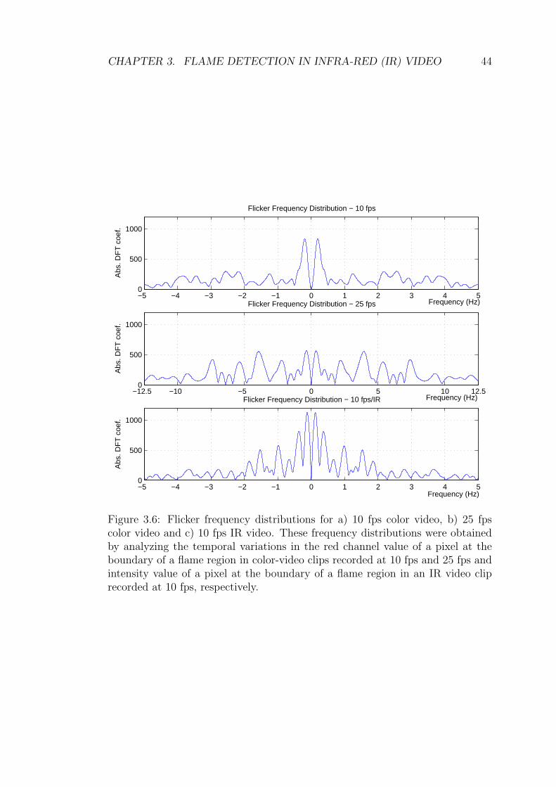
CHAPTER 3. FLAME DETECTION IN INFRA-RED (IR) VIDEO 44
−5 −4 −3 −2 −1 0 1 2 3 4 50
500
1000
Frequency (Hz)
Abs
. DF
T c
oef.
Flicker Frequency Distribution − 10 fps
−12.5 −10 −5 0 5 10 12.50
500
1000
Frequency (Hz)
Abs
. DF
T c
oef.
Flicker Frequency Distribution − 25 fps
−5 −4 −3 −2 −1 0 1 2 3 4 50
500
1000
Frequency (Hz)
Abs
. DF
T c
oef.
Flicker Frequency Distribution − 10 fps/IR
Figure 3.6: Flicker frequency distributions for a) 10 fps color video, b) 25 fpscolor video and c) 10 fps IR video. These frequency distributions were obtainedby analyzing the temporal variations in the red channel value of a pixel at theboundary of a flame region in color-video clips recorded at 10 fps and 25 fps andintensity value of a pixel at the boundary of a flame region in an IR video cliprecorded at 10 fps, respectively.

CHAPTER 3. FLAME DETECTION IN INFRA-RED (IR) VIDEO 45
Similar to the discussions in Chapter 2, flame flicker process in IR video is
characterized by a random Markov model. As in the previous chapter, three-
state Markov models are trained off-line for both flame and non-flame pixels to
represent the temporal behavior (cf. Fig. 4.3). These models are trained using a
feature signal which is defined as follows: Let Ik(n) be the intensity value of the
k − th pixel at frame n. The wavelet coefficients of Ik are obtained by the same
structure shown in Fig. 4.2, but filtering is implemented temporally.
Figure 3.7: Three-state Markov models for a) flame and b) non-flame movingpixels.
The states of HMMs are defined as follows: at time n, if |w(n)| < T1, the
state is in S1; if T1 < |w(n)| < T2, the state is S2; else if |w(n)| > T2, the state
S3 is attained. For the pixels of regular hot objects like walking people, engine
of a moving car, etc., no rapid changes take place in the pixel values. When the
wavelet coefficients fluctuate between values above the higher threshold T2 and
below the lower threshold T1 in a frequent manner this indicates the existence of
flames in the viewing range of the IR camera.
The transition probabilities between states for a pixel are estimated during a
pre-determined period of time around flame boundaries. During the recognition
phase, the HMM based analysis is carried out in pixels near the contour bound-
aries of bright moving regions whose ρ values exceed ρT . The state sequence of

CHAPTER 3. FLAME DETECTION IN INFRA-RED (IR) VIDEO 46
length 20 image frames is determined for these candidate pixels and fed to the
flame and non-flame pixel models. The model yielding higher probability is de-
termined as the result of the analysis for each of the candidate pixel. A pixel is
called as a flame or a non-flame pixel according to the result of this analysis. A
fire mask composing of flame pixels is formed as the output of the method.
3.3 Experimental Results
The proposed method was implemented in a personal computer with an AMD
AthlonXP 2000+ 1.66GHz processor. The HMMs used in the temporal analysis
step were trained using outdoor IR video clips with fire and ordinary moving
bright objects like people and cars. Video clips have 236577 image frames with
160 by 120 pixel resolution. All of the clips are captured at 10 fps using a cooled
long-wave IR camera with a spectral range of 8-12 µm. This camera has a longer
range than 30 meters up to which distance the proposed algorithm is developed
for. We cannot detect a starting fire in longer distances using the proposed
algorithm, because flame flicker cannot be observed in long distances.
There are moving cars and walking people in most of the test video clips.
Image frames from some of the clips are shown in Figs. 3.8 and 3.9. To increase
the number of videos in experimental studies, black and white video clips are also
used.
We used some of our clips for training the Markov models. The fire model was
trained with fire videos and the other model was trained with ordinary moving
bright objects. The remaining 48 video clips were used for test purposes. Our
method yields no false positives in any of the IR test clips.
A modified version of a recent method by Guillemant and Vicente [36] for
real-time identification of smoke in black and white video is implemented for
comparison. This method is developed for forest fire detection from watch tow-
ers. In a forest fire, smoke rises first, therefore, the method was tuned for smoke
detection. Guillemant and Vicente based their method on the observation that

CHAPTER 3. FLAME DETECTION IN INFRA-RED (IR) VIDEO 47
Figure 3.8: Image frames from some of the test clips. a), b) and c) Fire regionsare detected and flame boundaries are marked with arrows. d), e) and f) No falsealarms are issued for ordinary moving bright objects.

CHAPTER 3. FLAME DETECTION IN INFRA-RED (IR) VIDEO 48
Figure 3.9: Image frames from some of the test clips with fire. Pixels on theflame boundaries are successfully detected.

CHAPTER 3. FLAME DETECTION IN INFRA-RED (IR) VIDEO 49
the movements of various patterns like smoke plumes produce correlated tempo-
ral segments of gray-level pixels, which they called as temporal signatures. For
each pixel inside an envelope of possible smoke regions, they recovered its last d
luminance values to form a point P = [x0, x1, ..., xd−1] in d-dimensional “embed-
ding space”. Luminance values were quantized to 2e levels. They utilized fractal
indexing using a space-filling Z-curve concept whose fractal rank is defined as:
z(P ) =e−1∑j=0
d−1∑
l=0
2l+jdxjl (3.4)
where xjl is the j − th bit of xl for a point P . They defined an instantaneous ve-
locity for each point P using the linked-list obtained according to Z-curve fractal
ranks. After this step, they estimated a cumulative velocity histogram (CVH)
for each possible smoke region by including the maximum velocity among them
and made smoke decisions about the existence of smoke according to the stan-
dard deviation, minimum average energy, and shape and smoothness of these
histograms [36].
Our aim is to detect flames in manufacturing and power plants, large audito-
riums, and other large indoor environments. So, we modified the method in [36]
similar to the approach presented in Sec. 2.2. For comparison purposes, we re-
placed our wavelet-based contour analysis step with the CVH based method and
leave the rest of the algorithm as proposed. We formed two three-state Markov
models for flame and non-flame bright moving regions. These models were trained
for each possible flame region using wavelet coefficients of CVH standard devia-
tion values. States of HMMs were defined as in Sec. 3.2.2.
Comparative detection results for some of the test videos are presented in Ta-
ble 3.1. The second column lists the number of frames in which flames exist in
the viewing range of the camera. The third and fourth columns show the number
of frames in which flames were detected by the modified CVH method explained
in the above paragraph, and our method, respectively. Our method detected
flame boundaries that have irregular shapes both temporally and spatially. Both
methods detected fire in video clips V3–V6 and V8–V12 which contain actual
fires indoor and outdoor. In video clip V3, flames were behind a wall most of the

CHAPTER 3. FLAME DETECTION IN INFRA-RED (IR) VIDEO 50
time. The distance between the camera and fire ranges between 5 to 50 meters
in these video clips. Video clips V1, V2, and V7 do not contain any fire. There
are flames and walking people in the remaining clips. Some flame frames are
missed by both methods but this is not an important problem at all, because
the fire was detected in the next frame or the frame after the next one. The
method using CVH detected fire in most of the frames in fire containing videos,
as well. However, it yielded false alarms in clips V1, V7 and V9–V12, in which
there were a group of people walking by a car and around fire place. Proposed
method analyzes the contours of possible fire regions in wavelet domain. This
makes it more robust to slight contour changes than the modified method which
basically depends on the analysis of motion vectors of possible fire regions.
Flames of various burning materials have similar yet different temporal and
spatial characteristics. For example, oil flame has a peak flicker frequency around
15 Hz whereas it is around 5 Hz for coal flame (cf. Fig. 2 in [5]). In fact, flames
of the same burning material under different weather/wind conditions have also
different temporal and spatial characteristics. What is common among various
flame types is the wide-band random nature in them causing temporal and spatial
flicker. Our method exploits this stochastic nature. We use wavelet based feature
signals obtained from flickering flames to train and test our models in order to get
rid of the effects of specific conditions forming the flames. The wavelet domain
feature signals capture the condition-independent random nature of flames.
To verify the performance of our method with respect to flames of different
materials, we set up the following experiment:
1. We train the model with ‘paper’ fire and test it with both ‘paper’ and
‘paper + alcohol’ fires.
2. We train the model with ‘paper + alcohol’ fire and test it with both ‘paper’
and ‘paper + alcohol’ fires.
The results of this experiment for some of the test clips are presented in
Table 3.2. The results show that the method has similar detection rates for
different fires when trained with different flame types.

CHAPTER 3. FLAME DETECTION IN INFRA-RED (IR) VIDEO 51
Table 3.1: Detection results for some of the test clips. In the video clip V3, flamesare hindered by a wall for most of the time.
Number of frames Number of falseVideo Number of frames in which flames detected positive framesclips with flames CVH Method Our Method CVH Method Our MethodV1 0 17 0 17 0V2 0 0 0 0 0V3 71 42 63 0 0V4 86 71 85 0 0V5 44 30 41 0 0V6 79 79 79 0 0V7 0 15 0 15 0V8 101 86 101 0 0V9 62 52 59 8 0V10 725 510 718 54 0V11 1456 1291 1449 107 0V12 988 806 981 19 0
The proposed method was also tested with regular video recordings in com-
parison with the modified version of the method in [36] and the fire detection
method described in [87]. The method in [87] uses frequency subband analysis to
detect 10 Hz flame flicker, instead of using HMMs to capture the random tempo-
ral behavior in flames. Results for some of the clips are presented in Table 3.3.
The clip V17 does not contain any fire, either. However it leads to false alarms
because a man with bright fire colored shirt dances in front of the camera to fool
the algorithm. This man would not cause any false alarms if an infrared camera
were used instead of a regular visible range camera.
It should also be noted that, the proposed method is computationally more
efficient than [36] because it is mostly based on contour analysis of the bright
moving objects. Average processing time per frame for the proposed method is
5 msec as shown in Table 3.3.

CHAPTER 3. FLAME DETECTION IN INFRA-RED (IR) VIDEO 52
Table 3.2: Fire detection results of our method when trained with different flametypes.
Number of framesVideo Flame Number of frames in which flames detected byclips type with flames Our Method trained with
Paper fire Paper+alcohol fireV9 Paper 62 60 58V10 Paper 725 722 722V11 Paper+alcohol 1456 1449 1453V12 Paper+alcohol 993 988 991V13 Paper+alcohol 1434 1426 1430V14 Paper 999 996 995
Table 3.3: Comparison of the proposed method with the modified version of themethod in [36] (CVH method) and the fire detection method described in [87]for fire detection using a regular visible range camera. The values for processingtimes per frame are in milliseconds.
Number of frames Processing timeVideo Number of frames in which flames detected per frame (msec)clips with flames Our Method CVH Our Method CVH
Method in [87] Method Method in [87] MethodV15 37 31 37 26 5 16 11V16 18 13 18 8 5 17 10V17 0 2 9 7 4 16 10
3.4 Summary
A novel method to detect flames in IR video is developed. The algorithm uses
brightness and motion clues along with a temporal and a contour analysis in
wavelet domain. The main contribution of the method is the utilization of hidden
Markov models trained using temporal wavelet domain information to detect
random flicker process. The high frequency behavior of flame region boundaries
are analyzed using a wavelet based contour analysis technique. The experimental
results indicate that when the fire falls into the viewing range of an IR camera,
the proposed method is successful in detecting the flames without producing false
CHAPTER 3. FLAME DETECTION IN INFRA-RED (IR) VIDEO 53
alarms in all the examples that we tried. The method can be used for both indoor
and outdoor early fire detection applications.

Chapter 4
Short Range Smoke Detection in
Video
Smoldering smoke appears before flames in most fires. In addition, the source
of the fire and flames cannot always fall into the field of view of a camera or
a sensor monitoring an area of interest. Long Wave Infra-Red (LWIR) cameras
and pyro-electric infra-red (PIR) sensors which are used in flame detection are
not suitable for smoke detection. Contrary to the common belief, smoke cannot
be visualized in 8 − 12µm range LWIR cameras and sensors including Forward
Looking Infra-Red (FLIR) cameras and PIR sensors [76, 44]. However, smoke of
an uncontrolled fire can be easily observed by a visible range camera even if flames
are not visible. This results in early detection of fire before it spreads around.
This is vital for fire alarm systems when large and open areas are monitored.
A novel method to detect smoke in video is described in this chapter. The
chapter begins with the introduction of the video smoke detection method. In
Section 4.3, contour analysis is described. Experimental results are presented in
Chapter 4.4.
54

CHAPTER 4. SHORT RANGE SMOKE DETECTION IN VIDEO 55
4.1 Detection Algorithm
The flames of a fire may not always fall into the visible range of the camera
monitoring a scene covering large areas like plane hangars or open spaces. Fire
detection systems should tackle with such situations by successful detection of
smoke without flame. In this chapter, temporal and spatial wavelet analysis as
well as an analysis of contours of possible smoke regions are carried out for smoke
detection.
Smoke gradually smoothen the edges in an image. This characteristic prop-
erty of smoke is a good indicator of its presence [52], [10]. Edges in an image
correspond to local extrema in wavelet domain. Degradation of sharpness in the
edges result in a decrease in the values of these extrema. However, these extrema
values corresponding to edges do not totally boil down to zero when there is
smoke in the scene. In fact, they simply loose some of their energy but they still
stay in their original locations, occluded partially by the semi-transparent smoke.
Independent of the fuel type, smoke naturally decrease the chrominance chan-
nels U and V values of pixels. Apart from this, as discussed in the previous
chapters, both flame and smoke are turbulent phenomena. Smoke regions have
time-varying boundaries similar to flame regions. Smoke partially covers and
uncovers background objects especially at the early stages of fire. Therefore, a
Markov model based modeling of turbulent smoke behavior is appropriate as in
flame detection. However, smoke boundaries move with a lower frequency at the
early stages of fire.
In addition to color and turbulent behavior analysis, boundaries of smoke
regions are also estimated in each video image frame. A one-dimensional curve
(1-D) representing the distance to the boundary from the center of mass of the
region is extracted for each smoke region. The wavelet transform of this 1-D
curve is computed and the high frequency nature of the contour of the smoke
region is determined using the energy of the wavelet signal. This spatial domain
clue is also combined with temporal clues to reach a final decision.

CHAPTER 4. SHORT RANGE SMOKE DETECTION IN VIDEO 56
Smoke detection algorithm consists of five steps: (i) moving pixels or regions
in the current frame of a video are determined, (ii) the decrease in high frequency
content corresponding to edges in these regions are checked using spatial wavelet
transform. If edges loose their sharpness without vanishing completely (iii) the
U and V channel values corresponding to edge pixels are checked, (iv) turbulent
behavior analysis is carried out by HMMs which use temporal wavelet transform
coefficients. Finally, (v) object contours are analyzed in wavelet domain.
Moving objects in video are detected using the background estimation method
developed by Collins et al. [19]. This method assumes that the camera is sta-
tionary. Moving pixels are determined by subtracting the current image from the
background image and thresholding. A recursive threshold estimation is described
in [19].
In order to detect smoke, it is necessary to analyze moving regions in video
to determine if the motion is due to smoke or an ordinary moving object. Smoke
obstructs the texture and edges in the background of an image. Since edges
and texture contribute to the high frequency information of the image, energies
of wavelet sub-images drop due to smoke in an image sequence. Based on this
fact we monitor wavelet coefficients as in Fig. 4.1 and we detect decreases in
local wavelet energy, and detect individual wavelet coefficients corresponding to
edges of objects in background whose values decrease over time in video. It is
also possible to determine the location of smoke using the wavelet sub-images as
shown in Fig. 4.1.
Let Iv(x, y) = |ILH(x, y)| + |IHL(x, y)| + |IHH(x, y)| represent a composite
image containing high-frequency information corresponding to the image frame
I obtained by a single-level 2-D discrete wavelet transformation operation. In
order to make the analysis faster, this sub-band image is divided into small
blocks of size (K1, K2) and the energy eI(l1, l2) value of each block is computed
as eI(l1, l2) =∑
(x,y)∈RiIv(x + l1K1, y + l2K2) where Ri represents a block of
size (K1, K2) in the wavelet sub-image. If the wavelet sub-images are computed
from the luminance (Y) image, then there is no need to include the chrominance
wavelet images. If wavelet transforms of red (R), green (G), and blue (B) color

CHAPTER 4. SHORT RANGE SMOKE DETECTION IN VIDEO 57
Figure 4.1: Image frame with smoke and its single level wavelet sub-images.Blurring in the edges is visible. The analysis is carried out in small blocks.
images are computed, then the energy value, e(l1, l2), should be computed using
all wavelet sub-images of the R, G, and B color images. In our implementation,
sub-images are computed from the luminance image only and the block size is
taken as 8 by 8 pixels.
Let B represent a background image built-up in time according to the IIR-type
background update filter described in Section 2.2.1. Let Bv(x, y) = |BLH(x, y)|+|BHL(x, y)|+ |BHH(x, y)| represent a composite image containing high-frequency
information corresponding to the background image B obtained by the same
single-level 2-D discrete wavelet transformation operation as for Iv(x, y). In a
similar manner, local energy values, eB(l1, l2), of the composite image for the back-
ground image can be computed as eB(l1, l2) =∑
(x,y)∈RiBv(x + l1K1, y + l2K2)
where Ri represents a block of size (K1, K2) in the wavelet sub-image of the
background.
These local energy values, eI(l1, l2) and eB(l1, l2), corresponding to current
and background images are compared with each other. If there is a decrease in
energy value eB(l1, l2) of a certain block at location (l1, l2), then this means that
the texture or edges of the scene monitored by the camera no longer appear as
sharp in the current image of the video, as they used to be. Therefore, the image
region in the viewing range of the camera corresponding to (l1, l2)-th block could
be covered with smoke. One can set up thresholds for the comparison. If a certain
local background energy value eB(l1, l2) drops below a pre-determined threshold,

CHAPTER 4. SHORT RANGE SMOKE DETECTION IN VIDEO 58
a warning may be issued.
It is also well-known that wavelet sub-images contain the edge information
of the original image. Edges produce local extrema in wavelet sub-images [10].
Wavelet sub-images LH, HL and HH contains horizontal, vertical and diagonal
edges of the original image, respectively. If smoke covers one of the edges of
the original image then the edge initially becomes less visible and after some
time it may disappear from the scene as smoke gets thicker. Let the wavelet
coefficient IHL(x, y) be one of the wavelet coefficients corresponding to the edge
covered by smoke. Initially, its value decreases due to the reduced visibility,
and in subsequent image frames it becomes either zero or close to zero whenever
there is very little visibility due to thick smoke. Therefore locations of the edges
of the original image is determined from the significant extrema of the wavelet
transform of the background image in the proposed method. Slow fading of a
wavelet extrema is an important clue for smoke detection. If the values of a
group of wavelet coefficients along a curve corresponding to an edge decrease in
value in consecutive frames, then this means that there is less visibility in the
scene. In turn, this may be due to the existence of smoke.
An instantaneous disappearance or appearance of a wavelet extremum in the
current frame cannot be due to smoke. Such a change corresponds to an ordinary
moving object covering an edge in the background or the boundary of a moving
object and such changes are ignored.
Color information is also used for identifying smoke in video as the third step.
Initially, when smoke starts to expand, it is semi-transparent. Consequently, color
values of the pixels within semi-transparent smoke covered image regions decrease
with comparable rates. This in turn results in the preservation of the direction of
the vector defined by the RGB channel values. This is another clue for differenti-
ating between smoke and an ordinary moving object. By itself, this information
is not sufficient because shadows of moving objects also behave similarly. As
smoke gets thicker, however, the resemblance of the current image frame and the
background image decreases. The chrominance values U and V of the candidate
smoke pixels in the current frame gets smaller values than their corresponding

CHAPTER 4. SHORT RANGE SMOKE DETECTION IN VIDEO 59
Figure 4.2: Single-stage wavelet filter bank.
values in the background image.
The turbulent characteristic of smoke is also used as an additional informa-
tion. The candidate regions are checked whether they continuously appear and
disappear over time. In general, a pixel especially at the edge of a smoke becomes
part of smoke and disappears in the background several times in one second of a
video at random. This characteristic behavior is very well suited to be modeled
as a random Markov model.
Similar to flame detection methods presented in the previous chapters, three-
state Markov models are temporally trained for both smoke and non-smoke pixels
(cf.Fig.4.3) using a wavelet based feature signal. These models are trained using
a feature signal which is defined as follows: Let I(x, n) be the intensity value of
a pixel at location x in the image frame at time step n. The wavelet coefficients
of I are obtained by the filter bank structure shown in Fig.4.2. Non-negative
thresholds T1 < T2 introduced in wavelet domain, define the three states of the
hidden Markov models for smoke and non-smoke moving objects. At time n,
if |w(n)| < T1, the state is in F1; if T1 < |w(n)| < T2, the state is F2; else
if |w(n)| > T2, the state Out is attained. The transition probabilities between
states for a pixel are estimated during a pre-determined period of time around
smoke boundaries. In this way, the model not only learns the turbulent behavior
of smoke boundaries during a period of time, but also it tailors its parameters to
mimic the spatial characteristics of smoke regions.

CHAPTER 4. SHORT RANGE SMOKE DETECTION IN VIDEO 60
Figure 4.3: Three-state Markov models for smoke(left) and non-smoke movingpixels.
4.2 Wavelet Domain Analysis of Object Con-
tours
In addition to temporal and color analysis, contours of possible smoke regions
are further analyzed. For this purpose, the centers of masses of the moving
objects are determined. A one dimensional (1-D) signal is obtained by computing
the distance from the center of mass of the object to the object boundary for
0 ≤ θ < 2π. In Fig. 4.4, two image frames are shown. Example feature functions
of 64 equally spaced angles for moving vehicle and the fire region in Fig. 4.4 are
shown in Fig. 4.5. The high-frequency variations of the feature signal of smoke
region is clearly distinct from that of the car and lights.
To determine the high-frequency content of a curve, we use a single scale
wavelet transform shown in Fig. 4.2. The absolute wavelet (w) and low-band (c)
coefficients of smoke region and the moving car are shown in Figs. 4.6 and 4.7,
respectively. The ratio of the wavelet domain energy to the energy of the low-band
signal is a good indicator of a smoke region. This ratio is defined as ρ =∑
n |w[n]|∑n |c[n]| .
The likelihood of the moving region to be a smoke region is highly correlated with
the parameter ρ.
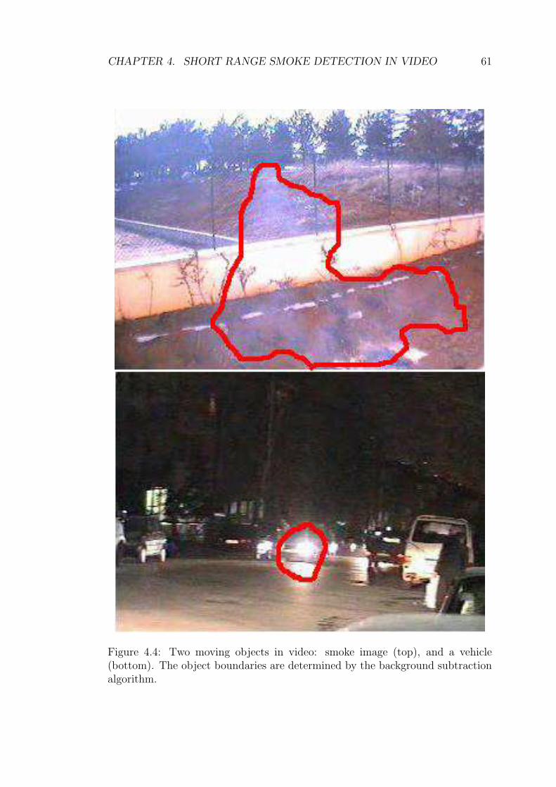
CHAPTER 4. SHORT RANGE SMOKE DETECTION IN VIDEO 61
Figure 4.4: Two moving objects in video: smoke image (top), and a vehicle(bottom). The object boundaries are determined by the background subtractionalgorithm.

CHAPTER 4. SHORT RANGE SMOKE DETECTION IN VIDEO 62
10 20 30 40 50 600
10
20
30
40
50a) Smoke Contour
10 20 30 40 50 600
10
20
30
40
50b) Vehicle and lights Contour
Figure 4.5: Equally spaced 64 contour points of smoke (top) and the vehicleregions (bottom) shown in Fig.4.4.

CHAPTER 4. SHORT RANGE SMOKE DETECTION IN VIDEO 63
5 10 15 20 25 300
1
2
3
4
5a) Smoke Contour Wavelet Coefs.
5 10 15 20 25 300
10
20
30
40
50b) Smoke Contour Low−band Coefs.
Figure 4.6: The absolute a) wavelet and b) low-band coefficients for the smokeregion.

CHAPTER 4. SHORT RANGE SMOKE DETECTION IN VIDEO 64
5 10 15 20 25 300
1
2
3
4
5a) Vehicle Contour Wavelet Coefs.
5 10 15 20 25 300
10
20
30
40
50b) Vehicle Contour Low−band Coefs.
Figure 4.7: The absolute a) wavelet and b) low-band coefficients for the vehicle.

CHAPTER 4. SHORT RANGE SMOKE DETECTION IN VIDEO 65
4.3 Experimental Results
The proposed method (Method-4.1) is implemented in a PC with an AMD
AthlonXP 2000+ 1.66GHz processor and tested for a large variety of conditions
including real-time and off-line videos containing only smoke, both flame and
smoke, and videos with no smoke or flame.
It is observed that, the proposed method is suitable for detection of smoke
in a range of up to 30m to the camera. This is due to the fact that as the
distance increases, the turbulent movements in smoke regions start to disappear
and become unobservable after a certain point. It is also hard to estimate the
contours of smoke regions at longer distances.
The computational cost of the wavelet transform is low. The filter-bank in
Fig. 4.2 have integer coefficient low and high-pass Lagrange filters. The same
filters are used for a single level wavelet decomposition of image frames in the
spatial wavelet analysis step and also for contour analysis. Smoke detection is
achieved in realtime. The processing time per frame is about 5 msec for frames
with sizes of 160 by 120 pixels.
Detection results for some of the test sequences are presented in Table 4.1.
Smoke is successfully detected in all of the shots containing smoke. No false
alarms are issued in live tests and off-line videos recorded in the day time. False
alarms are eliminated also for the videos recorded in the night with the help of
the contour analysis. A false alarm is issued with the method in [86], Method-4.2,
in Movie 9 which is recorded at night. A parking car is captured from its front in
this video. The driver intentionally varies the intensity of the front lights of the
car. The light beams directed towards the camera at night defines artificial edges
around them. These edges appear and disappear continuously as the intensity
of the lights change. The U,V channel values of the pixels decrease as the light
intensities are lowered, since everywhere in the scene is dark other than the car
lights. In this way, car lights at night mimic smoke characteristics in the day
time and a false alarm is issued using Method-4.2. However, using the method
proposed in this chapter (Method-4.1), this false alarm is eliminated, because

CHAPTER 4. SHORT RANGE SMOKE DETECTION IN VIDEO 66
the contour of the moving region defined by the car lights does not possess high
frequency characteristics as in a smoke region.
Proposed smoke detection method, Method-4.1, is also compared with the fire
detection method presented in [87], Method-4.3, in videos containing both smoke
and flame. The comparison results in some of the test sequences are presented
in Table 4.2. At the early stages of fire, smoke is released before flames become
visible. Method-4.1 successfully detects smoke in such situations earlier than
Method-4.3. Hence, early detection of fire is possible with the proposed smoke
detection method. In Movies 11 and 12, flames are not in the viewing range of
the camera. A fire detection system without smoke detection capability fails in
detecting the fire before it spread around.
Table 4.1: Detection results of Method-4.1 and Method-4.2 for some live andoff-line videos.
Number of ShotsVideo Number of shots detected as Smoke Description
Sequences with smoke Method-4.1 Method-4.2Movie 1 0 0 0 Smoke-colored parking carMovie 2 5 5 5 Fire in a gardenMovie 3 5 5 5 Fire in a garden in snowMovie 4 7 7 7 A burning boxMovie 5 6 6 6 A burning pile of woodsMovie 6 3 3 3 Fire in a waste-bin in the garden
monitored from an indoor cameraMovie 7 0 0 0 Three men walking in a roomMovie 8 8 8 8 Fire in a gardenMovie 9 0 0 1 A parking car in the night
4.4 Summary
In this chapter, a novel method for detecting short range smoke in visible range
video is developed. The algorithm is mainly based on determining the edge
regions whose wavelet sub-band energies decrease with time and wavelet based

CHAPTER 4. SHORT RANGE SMOKE DETECTION IN VIDEO 67
Table 4.2: Smoke and flame detection time comparison of Method-4.1 andMethod-4.3, respectively. Smoke is an early indicator of fire. In Movies 11 and12, flames are not in the viewing range of the camera.
Video Method Detection time DescriptionSequences (sec.)Movie 10 Method-4.1 3 Fire in a garden
Method-4.3 8Movie 11 Method-4.1 4 Fire in a trash bin
Method-4.3 N/AMovie 11 Method-4.1 7 Fire at a distance of 30m
Method-4.3 N/A
contour analysis of possible smoke regions. These regions are then analyzed
along with their corresponding background regions with respect to their RGB
and chrominance values. The turbulent behavior of smoke is also modeled with
Markov models and set as an additional clue for the final smoke decision.
The method can be used for detection of smoke in movies and video databases
as well as real-time detection of smoke. It can be incorporated with a surveillance
system monitoring an indoor or an outdoor area of interest for early detection of
fire. It can also be integrated with the flame detection method in [87] in order to
have a more robust video based fire detection system.

Chapter 5
Flame Detection Using PIR
Sensors
In this chapter, a flame detection system based on a pyroelectric (or passive)
infrared (PIR) sensor is described. Since the PIR sensor can be visualized as
a single-pixel camera, an algorithm similar to the (IR) video flame detection is
developed.
The fundamental property that is used in the methods described in Chapters
2 and 3 for is the random flicker of flames. As pointed out in Chapters 2 and 3,
flame flicker behavior is a wide-band activity. Similar behavior for flame flicker
are also reported in [82] and [7]. As a result, a Markov model based modeling of
flame flicker process produces more robust performance compared to frequency
domain based methods. In [82], several experiments on the relationship between
burner size and flame flicker frequency are presented. Recent research on pyro-IR
based combustion monitoring includes [7] in which a monitoring system using an
array of PIR detectors is realized.
A regular camera or typical IR flame sensors have a fire detection range of 30
meters. This is due to the fact that flicker in flames cannot be or sensed from
longer distances. Therefore, PIR based systems provide a cost-effective solution
to the fire detection problem in relatively large rooms as the unit cost of a camera
68

CHAPTER 5. FLAME DETECTION USING PIR SENSORS 69
based system or a regular IR sensor based system is in the order of one thousand
dollars.
In this chapter, wavelet domain signal processing is also used, which provides
robustness against sensor signal drift due to temperature variations in the ob-
served area. Regular temperature changes due to hot plates and radiators are
slow variations compared to the moving objects and flames. Since wavelet sub-
signals of a waveform are high-pass and band-pass in nature they do not get
affected by the slow variations.
Events are classified into two different classes in this approach. The first
class represents fire events, on the other hand, the second class represents non-
fire events. PIR sensor circuits are designed for detecting the movement of hot
objects. Therefore, we include regular human motion events such as walking or
running in the non-fire event class.
The PIR sensor can be considered as a single-pixel camera without loss of
generality. Therefore, the proposed PIR based fire detection algorithm is obtained
simply by removing the spatial analysis steps of the video flame detection methods
developed in Chapters 2 and 3.
Data acquisition and the PIR systems are described in the next Section. The
proposed algorithm and the experiments are presented in Sections 5.2 and 5.3,
respectively.
5.1 PIR Sensor System and Data Acquisition
Commercially available PIR sensor read-out circuits produce binary outputs.
However, it is possible to capture a continuous time analog signal indicating the
strength of the received signal in time. The corresponding circuit for capturing
an analog signal output is shown in Fig. 5.1.
The circuit consists of 4 operational amplifiers (op amps), IC1A, IC1B, IC1C
and IC1D. IC1A and B constitute a two stage amplifier circuit whereas IC1C
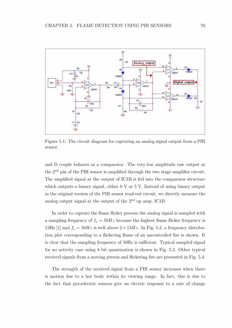
CHAPTER 5. FLAME DETECTION USING PIR SENSORS 70
Figure 5.1: The circuit diagram for capturing an analog signal output from a PIRsensor.
and D couple behaves as a comparator. The very-low amplitude raw output at
the 2nd pin of the PIR sensor is amplified through the two stage amplifier circuit.
The amplified signal at the output of IC1B is fed into the comparator structure
which outputs a binary signal, either 0 V or 5 V. Instead of using binary output
in the original version of the PIR sensor read-out circuit, we directly measure the
analog output signal at the output of the 2nd op amp, IC1B.
In order to capture the flame flicker process the analog signal is sampled with
a sampling frequency of fs = 50Hz because the highest flame flicker frequency is
13Hz [1] and fs = 50Hz is well above 2×13Hz. In Fig. 5.2, a frequency distribu-
tion plot corresponding to a flickering flame of an uncontrolled fire is shown. It
is clear that the sampling frequency of 50Hz is sufficient. Typical sampled signal
for no activity case using 8 bit quantization is shown in Fig. 5.3. Other typical
received signals from a moving person and flickering fire are presented in Fig. 5.4.
The strength of the received signal from a PIR sensor increases when there
is motion due to a hot body within its viewing range. In fact, this is due to
the fact that pyroelectric sensors give an electric response to a rate of change

CHAPTER 5. FLAME DETECTION USING PIR SENSORS 71
−25 −20 −15 −10 −5 0 5 10 15 20 250
1000
2000
3000
4000
5000
6000
7000
8000
9000
Frequency (Hz)
Abs
. DF
T c
oef.
Flicker Frequency Distribution
Figure 5.2: Flame flicker spectrum distribution. PIR signal is sampled with 50Hz.

CHAPTER 5. FLAME DETECTION USING PIR SENSORS 72
Figure 5.3: A typical PIR sensor output sampled at 50 Hz with 8 bit quantizationwhen there is no activity within its viewing range.

CHAPTER 5. FLAME DETECTION USING PIR SENSORS 73
(a)
(b)
Figure 5.4: PIR sensor output signals recorded at a distance of 5m for a (a)walking person, and (b) flame.

CHAPTER 5. FLAME DETECTION USING PIR SENSORS 74
of temperature rather than temperature itself. On the other hand, the motion
may be due to human motion taking place in front of the sensors or flickering
flame. In this chapter the PIR sensor data is used to distinguish the flame flicker
from the motion of a human being like running or walking. Typically the PIR
signal frequency of oscillation for a flickering flame is higher than that of PIR
signals caused by a moving hot body. In order to keep the computational cost
of the detection mechanism low, we decided to use Lagrange filters for obtaining
the wavelet transform coefficients as features instead of using a direct frequency
approach, such as FFT based methods.
5.2 Sensor Data Processing and HMMs
There is a bias in the PIR sensor output signal which changes according to the
room temperature. Wavelet transform of the PIR signal removes this bias. Let
x[n] be a sampled version of the signal coming out of a PIR sensor. Wavelet coef-
ficients obtained after a single stage subband decomposition, w[k], corresponding
to [12.5 Hz, 25 Hz] frequency band information of the original sensor output sig-
nal x[n] are evaluated with an integer arithmetic high-pass filter corresponding to
Lagrange wavelets [13] followed by decimation. The filter bank of a biorthogonal
wavelet transform is used in the analysis. The lowpass filter has the transfer
function:
Hl(z) =1
2+
1
4(z−1 + z1) (5.1)
and the corresponding high-pass filter has the transfer function
Hh(z) =1
2− 1
4(z−1 + z1) (5.2)
The term HMM is defined as “hidden-state” Markov model in Rabiner [67].
However, the term HMM is also used in a relaxed manner when several Markov
models are used to classify events. The term “hidden” refers to the fact that the
model producing the observed data is unknown.

CHAPTER 5. FLAME DETECTION USING PIR SENSORS 75
An HMM based classification is carried out for fire detection. Two three-state
Markov models are used to represent fire and non-fire events (cf. Fig. 6.2). In
these Markov models, state S1 corresponds to no activity within the viewing range
of the PIR sensor. The system remains in state S1 as long as there is not any
significant activity, which means that the absolute value of the current wavelet
coefficient, |w[k]|, is below a non-negative threshold T1. A second threshold T2
is also defined in wavelet domain which determines the state transitions between
S2 and S3. If T1 < |w[k]| < T2, then state S2 is attained. In case of |w[k]| > T2,
state S3 is acquired.
Figure 5.5: Two three-state Markov models are used to represent (a) ‘fire’ and(b) ‘non-fire’ classes, respectively.
The first step of the HMM based analysis consists of dividing the wavelet
coefficient sequences in windows of 25 samples. For each window, a corresponding
state transition sequence is determined. An example state transition sequence of
size 5 may look like
C = (S2, S1, S3, S2, S1) (5.3)
Since the wavelet signal captures the high frequency information in the signal,
we expect that there will be more transitions occurring between states when

CHAPTER 5. FLAME DETECTION USING PIR SENSORS 76
monitoring fire compared to human motion.
5.2.1 Threshold Estimation for State Transitions
The thresholds T1 and T2 in the wavelet domain determine the state transition
probabilities for a given sensor signal. In the training step, the task is to find
optimal values for T1 and T2. Given (T1, T2) and ground-truth fire and non-fire
wavelet training sequences, it is possible to calculate the transition probabilities
for each class. Let aij denote the transition probabilities for the ‘fire’ class and
bij denote the transition probabilities for the ‘non-fire’ class.
The decision about the class affiliation of a state transition sequence C of size
L is done by calculating the two joint probabilities Pa(C) and Pb(C) corresponding
to fire and non-fire classes, respectively:
Pa(C) =∏
i
pa(Ci+1|Ci) =∏
i
aCi,Ci+1(5.4)
and
Pb(C) =∏
i
pb(Ci+1|Ci) =∏
i
bCi,Ci+1(5.5)
where pa(Ci+1|Ci) = aCi,Ci+1, and pb(Ci+1|Ci) =
∏i bCi,Ci+1
, and i = 1, ..., L .
In case of Pa(C) > ξPb(C), for ξ > 0, the class affiliation of state transition
sequence C will be declared as ‘fire’, otherwise it is declared as ‘non-fire’. In our
implementation, we take ξ = 1 without loss of generality.
Given Na training sequences A1, ..., ANa from ‘fire’ class and Nb training se-
quences B1, ..., BNbfrom ‘non-fire’ class, the task of the training step is to find
the tuple (T1, T2) which maximizes the dissimilarity D = (Sa − Sb)2, where
Sa =∑
i Pa(Bi) and Sb =∑
i Pb(Ai).
This means that, for each given tuple (T1, T2), there is a specific value of the
dissimilarity D, so that D is a function of (T1, T2)
D = D(T1, T2) (5.6)
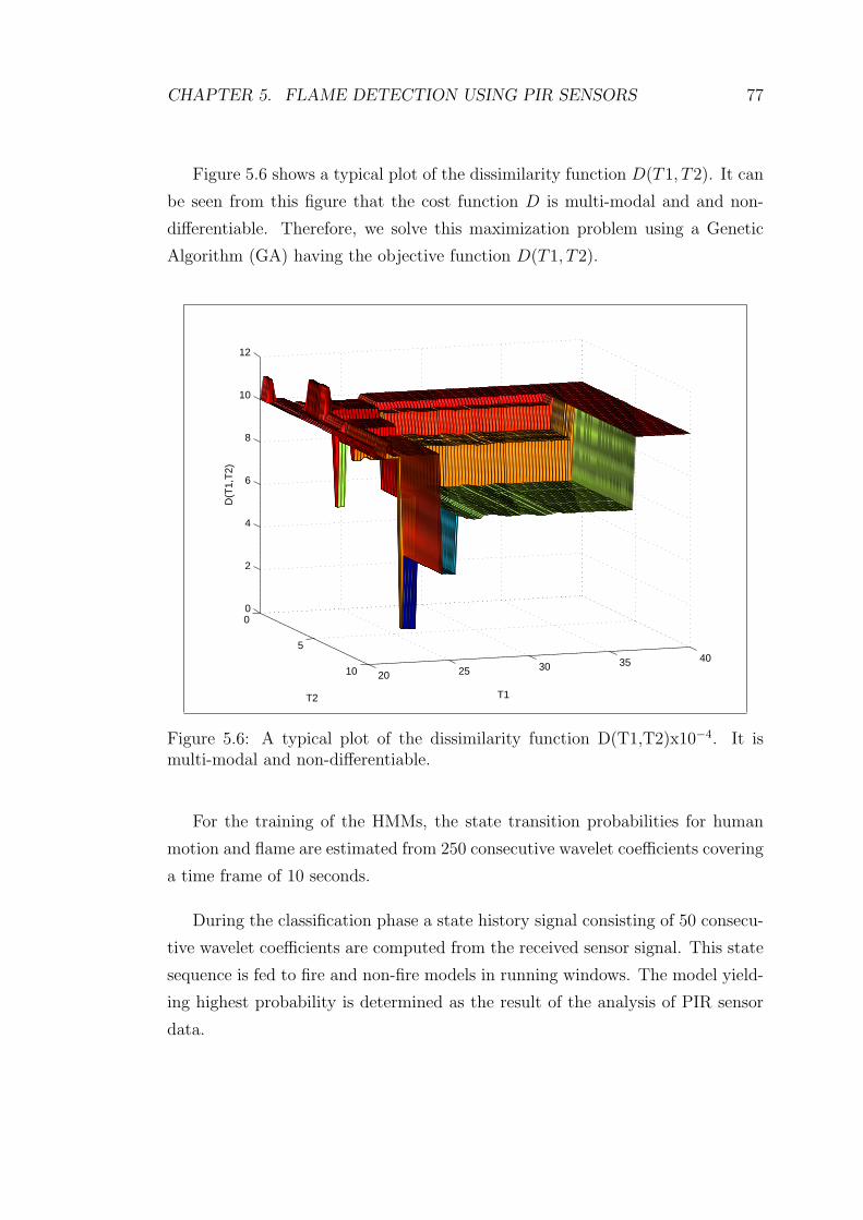
CHAPTER 5. FLAME DETECTION USING PIR SENSORS 77
Figure 5.6 shows a typical plot of the dissimilarity function D(T1, T2). It can
be seen from this figure that the cost function D is multi-modal and and non-
differentiable. Therefore, we solve this maximization problem using a Genetic
Algorithm (GA) having the objective function D(T1, T2).
0
5
10 20 25 30 35 40
0
2
4
6
8
10
12
T1T2
D(T
1,T
2)
Figure 5.6: A typical plot of the dissimilarity function D(T1,T2)x10−4. It ismulti-modal and non-differentiable.
For the training of the HMMs, the state transition probabilities for human
motion and flame are estimated from 250 consecutive wavelet coefficients covering
a time frame of 10 seconds.
During the classification phase a state history signal consisting of 50 consecu-
tive wavelet coefficients are computed from the received sensor signal. This state
sequence is fed to fire and non-fire models in running windows. The model yield-
ing highest probability is determined as the result of the analysis of PIR sensor
data.

CHAPTER 5. FLAME DETECTION USING PIR SENSORS 78
For flame sequences, the transition probabilities a′s should be high and close
to each other due to random nature of uncontrolled fire. On the other hand,
transition probabilities should be small in constant temperature moving bodies
like a walking person because there is no change or little change in PIR signal
values. Hence we expect a higher probability for b00 than any other b value in
the non-fire model which corresponds to higher probability of being in S1. The
state S2 provides hysteresis and it prevents sudden transitions from S1 to S3 or
vice versa.
5.3 Experimental Results
The analog output signal is sampled with a sampling frequency of 50 Hz and
quantized at 8 bits. Real-time analysis and classification methods are imple-
mented with C++ running on a PC. Digitized output signal is fed to the PC via
RS-232 serial port.
The detection range of a PIR sensor based system is 5 meters but this is
enough to cover most rooms with high ceilings. In our experiments we record
fire and non-fire sequences at a distance of 5m to the sensor, as well. For fire
sequences, we burn paper and alcohol, and record the output signals. For the
non-fire sequences, we record walking and running person sequences. The person
within the viewing range of the PIR sensor walks or runs on a straight line which
is tangent to the circle with a radius of 5m and the sensor being at the center.
The training set consists of 90 fire and 90 non-fire recordings with durations
varying between three to four seconds. The test set for fire class is 198 and that of
non-fire set is 558. Our method successfully detects fire for 195 of the sequences
in the fire test set. It does not trigger fire alarm for any of the sequences in the
non-fire test set. This is presented in Table 5.3.
The false negative alarms, 3 out of 198 fire test sequences, are issued for the
recordings where a man was also within the viewing range of the sensor along with
a fire close to diminish inside a waste-bin. The test setting where false alarms

CHAPTER 5. FLAME DETECTION USING PIR SENSORS 79
Table 5.1: Results with 198 fire, 588 non-fire test sequences. The system triggersan alarm when fire is detected within the viewing range of the PIR sensor.
No. of Sequences No. of False Alarms No. of AlarmsFire Test Sequences 198 3 195
Non-Fire Test Sequences 588 0 0
are issued is presented in Fig. 5.7.
5.4 Summary
In this chapter, a method for flame detection using PIR sensors is proposed.
Analog signal from a PIR sensor is sampled with a sampling frequency of 50 Hz
and quantized with 8 bits. Single level wavelet coefficients of the output signal
are used as feature vectors for flame detection.
PIR sensor output recordings containing various human movements and
flames of paper and alcohol fire at a range of 5m are used for training the HMMs
corresponding to different events. Thresholds for defining the states of HMMs
are estimated using an evolutionary algorithm, since the underlying cost function
to be minimized has proved to be multi-modal and non-differentiable. Flame de-
tection results of the proposed algorithm show that the single-pixel assumption
for PIR sensor proves to be a correct one.
This thesis demonstrates that low-cost PIR sensors which are commonly used
as indoor and outdoor motion detectors, can be utilized as fire sensors when
coupled with appropriate processing. The main advantage of a PIR based fire
detection system over conventional particle sensors is its ability to detect the
presence of fire from a distance which results in a faster response time.

CHAPTER 5. FLAME DETECTION USING PIR SENSORS 80
Figure 5.7: The PIR sensor is encircled. The fire is close to die out completely.A man is also within the viewing range of the sensor.

Chapter 6
Wildfire Detection
In this chapter, a computer vision based algorithm for wildfire detection is devel-
oped. The main detection algorithm is composed of four sub-algorithms detect-
ing (i) slow moving objects, (ii) smoke-colored regions, (iii) rising regions, and
(iv) shadows. Each sub-algorithm yields its own decision as a zero-mean real
number, representing the confidence level of that particular sub-algorithm. Con-
fidence values are linearly combined with weights determined according to a novel
active fusion method based on the least-mean-square (LMS) algorithm which is
a widely used technique in adaptive filtering. Weights are updated on-line using
the LMS method in the training (learning) stage. The error function of the LMS
based training process is defined as the difference between the weighted sum of
decision values and the decision of an oracle, who is the security guard of the
forest look-out tower. Simulation results are presented.
6.1 Related Work
Manned lookout posts are widely available in forests all around the world to detect
wild fires. Surveillance cameras can be placed on to these surveillance towers to
monitor the surrounding forestal area for possible wild fires. Furthermore, they
can be used to monitor the progress of the fire from remote centers.
81

CHAPTER 6. WILDFIRE DETECTION 82
In this chapter, a computer vision based method for wildfire detection is pre-
sented. Currently, average fire detection time is five minutes in manned lookout
towers in Turkey. Guards have to work 24 hours in remote locations under difficult
circumstances. They may get tired or leave the lookout tower for various reasons.
Therefore, computer vision based video analysis systems capable of producing
automatic fire alarms are necessary to reduce the average forest fire detection
time.
There are several approaches on automatic detection of forest fires in the
literature. Some of the approaches are directed towards detection of the flames
using infra-red and/or visible-range cameras and some others aim at detecting
the smoke due to wildfire [22] [46], [4] [36]. There are also recent papers on
sensor based detection of forest fires [39], [70]. Infrared cameras and sensor based
systems have the ability to capture the rise in temperature however they are much
more expensive compared to regular pan-tilt-zoom (PTZ) cameras.
It is almost impossible to view flames of a wildfire from a camera mounted
on a forest watch tower unless the fire is very near to the tower. However, smoke
rising up in the forest due to a fire is usually visible from long distances. A
snapshot of a typical wildfire smoke captured by a look-out tower camera from a
distance of 5 Km is shown in Fig. 6.1.
Guillemant and Vicente based their method on the observation that the move-
ments of various patterns like smoke plumes produce correlated temporal seg-
ments of gray-level pixels. They utilized fractal indexing using a space-filling
Z-curve concept along with instantaneous and cumulative velocity histograms for
possible smoke regions. They made smoke decisions about the existence of smoke
according to the standard deviation, minimum average energy, and shape and
smoothness of these histograms [36].
Smoke at far distances (> 100m to the camera) exhibits different spatio-
temporal characteristics than nearby smoke and fire [84], [23], [87]. This demands
specific methods explicitly developed for smoke detection at far distances rather
than using nearby smoke detection methods described in [86]. This approach is in
accordance with the ‘weak’ Artificial Intelligence (AI) framework [61] introduced

CHAPTER 6. WILDFIRE DETECTION 83
Figure 6.1: Snapshot of a typical wildfire smoke captured by a forest watch towerwhich is 5 km away from the fire (rising smoke is marked with an arrow).
by Hubert L. Dreyfus as opposed to ‘generalized’ AI. According to this framework
each specific problem in AI should be addressed as an individual engineering
problem with its own characteristics [25], [26].
The proposed automatic video based wildfire detection algorithm is based on
four sub-algorithms: (i) slow moving video object detection, (ii) smoke-colored
region detection, (iii) rising video object detection, (iv) shadow detection and
elimination. Each sub-algorithm decides on the existence of smoke in the viewing
range of the camera separately. Decisions from sub-algorithms are combined to-
gether by an adaptive active fusion method. Initial weights of the sub-algorithms
CHAPTER 6. WILDFIRE DETECTION 84
are determined from actual forest fire videos and test fires. They are updated us-
ing the least-mean-square (LMS) algorithm during initial installation. The LMS
algorithm was initially developed by Widrow in 1960’s together with neural net-
works [91]. The error function in the LMS adaptation is defined as the difference
between the overall decision of the compound algorithm and the decision of an
oracle. In our case, the oracle is the security guard. The compound decision al-
gorithm will obviously produce false alarms. The system asks the guard to verify
its decision whenever an alarm occurs. In this way, the user actively participate
in the learning process.
The chapter is organized as follows: Section 6.2 describes briefly each one
of the four sub-algorithms which make up the compound (main) wildfire detec-
tion algorithm. Adaptive active fusion method is described in Section 6.3. In
Section 6.4, experimental results are presented and the proposed online active
fusion method is compared with the universal linear predictor and the weighted
majority algorithms. Finally, conclusions are drawn in Section 6.5.
6.2 Building Blocks of Wildfire Detection Algo-
rithm
Wildfire detection algorithm is developed to recognize the existence of wildfire
smoke within the viewing range of the camera monitoring forestal areas. The pro-
posed wildfire smoke detection algorithm consists of four main sub-algorithms:
(i) slow moving object detection in video, (ii) smoke-colored region detection,
(iii) rising video object detection, (iv) shadow detection and elimination of shadow
regions, with decision functions, D1(x, n), D2(x, n), D3(x, n) and D4(x, n), re-
spectively, for each pixel at location x of every incoming image frame at time
step n. Computationally efficient sub-algorithms are selected in order to realize
a real-time wildfire detection system working in a standard PC.
Decision functions Di, i = 1, ..., M of sub-algorithms do not produce binary
values 1 (correct) or −1 (false), but they produce zero-mean real numbers for

CHAPTER 6. WILDFIRE DETECTION 85
each incoming sample x. If the number is positive (negative), then the individual
algorithm decides that there is (not) smoke due to forest fire in the viewing range
of the camera. Output values of decision functions express the confidence level
of each sub-algorithm. Higher the value, the more confident the algorithm.
6.2.1 Detection of Slow Moving Objects
Video objects at far distances to the camera seem to move slower (px/sec) in
comparison to the nearby objects moving at the same speed. Assuming the
camera is fixed, two background images, Bfast(x, n) and Bslow(x, n) corresponding
to the scene with different update rates are estimated [9], [65], where x is the
location of the pixel at frame number n.
In [19] a background image B(x, n + 1) at time instant n + 1 is recursively
estimated from the image frame I(x, n) and the background image B(x, n) of the
video as follows:
B(x, n + 1) =
{aB(x, n) + (1− a)I(x, n) if x is stationary
B(x, n) if x is a moving pixel(6.1)
where I(x, n) represent the intensity value of the pixel at location x in the nth
video frame I, and a is a parameter between 0 and 1. Initially, Bfast(x, 0) and
Bslow(x, 0) can be taken as I(x, 0). Stationary and moving pixel definitions are
given in [19]. Background images Bfast(x, n) and Bslow(x, n) are updated as in
Eq. 6.1 with different update rates. In our implementation, Bfast(x, n) is updated
at every frame and Bslow(x, n) is updated once in a second with a = 0.7 and 0.9,
respectively.
Slow moving objects within the viewing range of the camera are detected by
comparing background images, Bfast and Bslow [83], [9], [65]. If there exists a
substantial difference between the two images for some period of time, then an
alarm for slow moving region is raised, and the region is marked.
The decision value indicating the confidence level of the first sub-algorithm is
determined by the difference between background images. The decision function
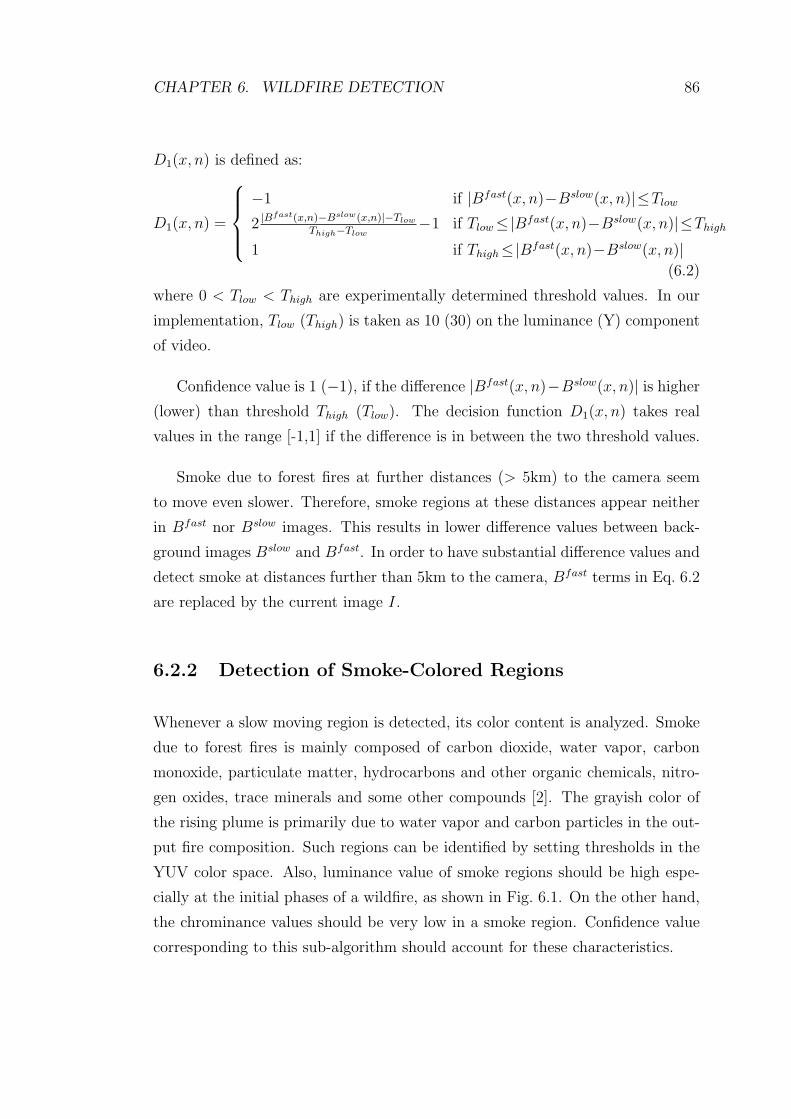
CHAPTER 6. WILDFIRE DETECTION 86
D1(x, n) is defined as:
D1(x, n) =
−1 if |Bfast(x, n)−Bslow(x, n)|≤Tlow
2 |Bfast(x,n)−Bslow(x,n)|−Tlow
Thigh−Tlow−1 if Tlow≤|Bfast(x, n)−Bslow(x, n)|≤Thigh
1 if Thigh≤|Bfast(x, n)−Bslow(x, n)|(6.2)
where 0 < Tlow < Thigh are experimentally determined threshold values. In our
implementation, Tlow (Thigh) is taken as 10 (30) on the luminance (Y) component
of video.
Confidence value is 1 (−1), if the difference |Bfast(x, n)−Bslow(x, n)| is higher
(lower) than threshold Thigh (Tlow). The decision function D1(x, n) takes real
values in the range [-1,1] if the difference is in between the two threshold values.
Smoke due to forest fires at further distances (> 5km) to the camera seem
to move even slower. Therefore, smoke regions at these distances appear neither
in Bfast nor Bslow images. This results in lower difference values between back-
ground images Bslow and Bfast. In order to have substantial difference values and
detect smoke at distances further than 5km to the camera, Bfast terms in Eq. 6.2
are replaced by the current image I.
6.2.2 Detection of Smoke-Colored Regions
Whenever a slow moving region is detected, its color content is analyzed. Smoke
due to forest fires is mainly composed of carbon dioxide, water vapor, carbon
monoxide, particulate matter, hydrocarbons and other organic chemicals, nitro-
gen oxides, trace minerals and some other compounds [2]. The grayish color of
the rising plume is primarily due to water vapor and carbon particles in the out-
put fire composition. Such regions can be identified by setting thresholds in the
YUV color space. Also, luminance value of smoke regions should be high espe-
cially at the initial phases of a wildfire, as shown in Fig. 6.1. On the other hand,
the chrominance values should be very low in a smoke region. Confidence value
corresponding to this sub-algorithm should account for these characteristics.
CHAPTER 6. WILDFIRE DETECTION 87
The decision function D2(x, n) takes values between 1 and −1 depending
on the values of the Y (x, n), U(x, n) and V (x, n) channel values. The decision
function D2(x, n) is defined as:
D2(x, n) =
{1− |U(x,n)−128|+|V (x,n)−128|
128, if Y (x, n) > TI
−1, otherwise(6.3)
where Y (x, n), U(x, n) and V (x, n) are the luminance and chrominance values of
the pixel at location x of the input image frame at time step n, respectively. The
luminance component Y takes real values in the range [0, 255] in an image and
the mean values of chrominance channels, U and V are increased to 128 so that
they also take values between 0 and 255. The threshold TI is an experimentally
determined value and taken as 100 on the luminance (Y) component in this
work. The confidence level of D2(x, n) is −1 if Y (x, n) is below TI . The reason
that we have the threshold TI is to eliminate dark regions which also have low
chrominance values. Since wildfire smoke regions are mostly colorless, having very
low chrominance values, the decision value approaches to 1 as the chrominance
values U(x, n) and V (x, n) are around the mean value of 128 for pixels whose
luminance values are greater than TI . Confidence value drops down to −1 for
pixels with high chrominance values.
6.2.3 Detection of Rising Regions
Wildfire smoke regions tend to rise up into the sky at the early stages of the fire.
This characteristic behavior of smoke plumes is modeled with three-state Hidden
Markov Models (HMM) in this chapter. Temporal variation in row number of the
upper-most pixel belonging to a slow moving region is used as a one dimensional
(1-D) feature signal, F = f(n), and fed to the Markov models shown in Fig.6.2.
One of the models (λ1) corresponds to genuine wildfire smoke regions and the
other one (λ2) corresponds to regions with clouds and cloud shadows. Transition
probabilities of these models are estimated off-line from actual wildfires and test
fires, and clouds. The state S1 is attained, if the row value of the upper-most pixel
in the current image frame is smaller than that of the previous frame (rise-up).
If the row value of the upper-most pixel in the current image frame is larger than

CHAPTER 6. WILDFIRE DETECTION 88
that of the previous frame, then S2 is attained and this means that the region
moves-down. No change in the row value corresponds to S3.
Figure 6.2: Markov model λ1 corresponding to wildfire smoke (left) and theMarkov model λ2 of clouds (right). Transition probabilities aij and bij are esti-mated off-line.
A slow moving region is classified as a rising region when the probability of
obtaining the observed feature signal F = f(n) given the probability model λ1
is greater than the probability of obtaining the observed feature signal F = f(n)
given the probability model λ2, i.e., when the upper-most pixel belonging to a
slow moving region tends to exhibit a rising characteristic:
p1 = P (F |λ1) > p2 = P (F |λ2) (6.4)
where F is the observed feature signal, λ1 and λ2 represent the Markov models
for wildfire smoke and clouds, respectively.
As the probability p1 (p2) gets a larger value than p2 (p1), the confidence level
of this sub-algorithm increases (decreases). Therefore, the zero-mean decision
function D3(x, n) is determined by the normalized difference of these probabilities:
D3(x, n) =p1 − p2
p1 + p2
(6.5)

CHAPTER 6. WILDFIRE DETECTION 89
When a slow moving region is classified as a rising region, i.e., p1 À p2, D3(x, n)
is close to 1. Otherwise, the decision function D3(x, n) is close to −1.
6.2.4 Shadow Detection and Removal
Shadows of slow moving clouds are major source of false alarms for video based
wildfire smoke detection systems. Unfortunately, shadows of clouds have very
low U and V values, similar to smoke regions due to wildfires.
The decision function for shadow regions are defined based on the shadow
detection method described in [41]. Average RGB values are calculated for slow
moving regions both in the current and the background images. Let S(n) repre-
sent a slow moving region in the image I at frame number n. The average color
vector, ~cI,S(n), of this region in the image I at frame number n is calculated as
follows:
~cI,S(n) =1
AS(n)
(∑
x∈S(n)
rI(x, n),∑
x∈S(n)
gI(x, n),∑
x∈S(n)
bI(x, n)) (6.6)
where AS(n) is the area of the slow moving region S(n), and rI(x, n), gI(x, n),
and bI(x, n) are the red, green and blue channel values of the pixel at location x
in the n − th image frame I. Similarly, average color vector, ~cB,S, of the same
region in the background image, B, is calculated as follows:
~cB,S(n) =1
AS(n)
(∑
x∈S(n)
rB(x, n),∑
x∈S(n)
gB(x, n),∑
x∈S(n)
bB(x, n)) (6.7)
where rB(x, n), gB(x, n), and bB(x, n) are the red, green and blue channel values of
the pixel at location x in the background image frame B at frame number n. We
used the background image Bslow as the background image in our implementation.
In shadow regions, the angle, θ(x), between the average color vectors, ~cI,S
and ~cB,S, should be small and the magnitude of the vector in the current im-
age should be smaller than that of the vector in the background image, i.e.,
| ~cI,S(n)| < | ~cB,S(n)| [41]. This is because shadow regions retain the color and
the underlying texture to some extent.

CHAPTER 6. WILDFIRE DETECTION 90
The confidence value of this sub-algorithm is defined according to the angle
and magnitudes of average color vectors, ~cI,S(n) and ~cB,S(n). The decision func-
tion D4(x, n) corresponding to this sub-algorithm for a pixel in the n− th image
and background frames is given by:
D4(x, n) =
{4|θ(x)|
π− 1, if | ~cI,S(n)| < | ~cB,S(n)|
−1, if | ~cI,S(n)| > | ~cB,S(n)|(6.8)
where θ(x) is the angle between the two color vectors. When the angle between
the two color vectors are close to each other, the function D4(x, n) is close to
−1 which corresponds to shadow regions. Similar decision functions for shadow
detection can be defined according to other color spaces including the Y UV space.
There are other shadow detection algorithms in the literature [66]. However,
we selected the algorithm described in this section, because of its low computa-
tional complexity. Our aim is to realize a wildfire detection system working in
real-time.
The threshold values in all of the decision functions described in this section
are chosen in such a way that they produce positive values for all of the wild fire
video recordings that we have. Still, one can define other sets of decision functions
with different threshold values representing various threat/security levels. In the
standard monitoring mode without any fires in the viewing range of the cameras,
the security level may be kept as ‘low’. Once a fire is detected, the system
can automatically switch to security level ‘high’ and increase the probability of
detecting possible fires that may follow the initial one, by lowering the thresholds
in the decision functions.
Decision results of four sub-algorithms, D1, D2, D3 and D4 are linearly com-
bined to reach a final decision on a given pixel whether it is a pixel of a smoke
region or not. Equal weights could be assigned to each sub-algorithm, however,
this would yield a non-adaptive algorithm without any learning capability. On
the other hand, wildfire detection is actually a dynamic process. There may
be wild variations between forestal areas and substantial temporal changes may
occur within the same forestal region. An adaptive combination of different sub-
algorithms would be more appropriate for robust wildfire detection. In the next

CHAPTER 6. WILDFIRE DETECTION 91
section the adaptive active learning algorithm will be discussed.
6.3 Adaptation of Sub-algorithm Weights
Cameras, once installed, operate at forest watch towers throughout the fire season
for about six months. There is usually a guard in charge of the cameras, as well.
The guard can supply feed-back to the detection algorithm after the installation of
the system. Whenever an alarm is issued, she/he can verify it or reject it. In this
way, she/he can participate the learning process of the adaptive algorithm. The
proposed active fusion algorithm can be also used in other supervised learning
problems.
As described in the previous section, the main wildfire detection algorithm is
composed of four sub-algorithms. Each algorithm has its own decision function
yielding a zero-mean real number for slow moving regions at every image frame of
a video sequence. Decision values from sub-algorithms are linearly combined and
weights of sub-algorithms are adaptively updated in our approach. Sub-algorithm
weights are updated according to the least-mean-square (LMS) algorithm which
is by far the most widely used adaptive filtering method [37], [93]. It also finds
applications in general classification and pattern recognition problems [27]. How-
ever, to the best of our knowledge, this thesis is the first example of an LMS
based approach introduced in an online active learning framework. Due to the
tracking capability of the algorithm, the proposed framework for online active
decision fusion may find applications in problems with drifting concepts.
Another innovation that we introduced in this chapter is that individual deci-
sion algorithms do not produce binary values 1 (correct) or −1 (false), but they
produce a zero-mean real number. If the number is positive (negative), then the
individual algorithm decides that there is (not) smoke due to forest fire in the
viewing range of the camera. Higher the absolute value, the more confident the
sub-algorithm.
Let the compound algorithm be composed of M -many detection algorithms:

CHAPTER 6. WILDFIRE DETECTION 92
D1, ..., DM . Upon receiving a sample input x, each algorithm yields a zero-mean
decision value Di(x) ∈ R. The type of the sample input x may vary depending
on the algorithm. It may be an individual pixel, or an image region, or the entire
image depending on the sub-algorithm of the computer vision problem. In the
wildfire detection problem the number of sub-algorithms, M=4 and each pixel at
the location x of incoming image frame is considered as a sample input for every
detection algorithm.
Let D(x, n) = [D1(x, n)...DM(x, n)]T , be the vector of confidence values of
the sub-algorithms for the pixel at location x of input image frame at time step
n, and w(n) = [w1(n)...wM(n)]T be the current weight vector.
We define
y(x, n) = DT(x, n)w(n) =∑
i
wi(n)Di(x, n) (6.9)
as an estimate of the correct classification result y(x, n) of the oracle for the
pixel at location x of input image frame at time step n, and the error e(x, n) as
e(x, n) = y(x, n)− y(x, n). Weights are updated by minimizing the mean-square-
error (MSE):
minwi
E[(y(x, n)− y(x, n))2], i = 1, ..., M (6.10)
where E represents the expectation operator. Taking the derivative with respect
to weights:
∂E
∂wi
= −2E[(y(x, n)− y(x, n))Di(x, n)] = −2E[e(x, n)Di(x, n)], i = 1, ..., M
(6.11)
and setting the result to zero:
−2E[e(x, n)Di(x, n)] = 0, i = 1, ..., M (6.12)
a set of M equations is obtained. The solution of this set of equations is called the
Wiener solution [37], [93]. Unfortunately, the solution requires the computation
of cross-correlation terms in Eq. 6.12. The gradient in Eq. 6.11 can be used in
a steepest descent algorithm to obtain an iterative solution to the minimization
problem in Eq. 6.10 as follows:
w(n + 1) = w(n) + λE[e(x, n)D(x, n)] (6.13)

CHAPTER 6. WILDFIRE DETECTION 93
where λ is a step size. In the well-known LMS algorithm, the ensemble average
E[e(x, n)D(x, n)] is estimated using the instantaneous value e(x, n)D(x, n) or it
can be estimated from previously processed pixels as follows:
e(x, n)D(x, n)] =1
L
∑x,n
e(x, n)D(x, n) (6.14)
where L is the number of previously processed pixels which is equal to the number
of terms inside the summation. The LMS algorithm is derived by noting that
the quantity in Eq. 6.13 is not available but its instantaneous value is easily
computable, and hence the expectation is simply replaced by its instantaneous
value [73]:
w(n + 1) = w(n) + λe(x, n)D(x, n) (6.15)
Eq. 6.15 is a computable weight-update equation. Whenever the oracle provides
a decision, the error e(x, n) is computed and the weights are updated according
to Eq. 6.15. Note that, the oracle does not assign her/his decision to each and
every pixel one by one. She/he actually selects a window on the image frame and
assigns a “1” or “−1” to the selected window.
Convergence of the LMS algorithm can be analyzed based on the MSE surface:
E[e2(x, n)] = Py(x, n)− 2wTp−wTRw (6.16)
where Py = E[y2(x, n)], p = E[y(x, n)D(x, n)], and R = E[D(x, n)DT (x, n)],
with the assumption that y(x, n) and D(x, n) are wide-sense-stationary random
processes. The MSE surface is a function of the weight vector w. Since E[e2(x, n)]
is a quadratic function of w, it has a single global minimum and no local minima.
Therefore, the steepest descent algorithm of Eqs. 6.13 and 6.15 is guaranteed to
converge to the Wiener solution, w∗ [73] with the following condition on the step
size λ [93]:
0 < λ <1
αmax
(6.17)
where αmax is the largest eigenvalue of R.
In Eq. 6.15, the step size λ can be replaced by
µ
||D(x, n)||2 (6.18)

CHAPTER 6. WILDFIRE DETECTION 94
as in the normalized LMS algorithm, which leads to:
w(n + 1) = w(n) + µe(x, n)
||D(x, n)||2D(x, n) (6.19)
where the µ is an update parameter and the normalized LMS algorithm converges
for 0 < µ < 2 to the Wiener solution, w∗ with the wide-sense-stationarity as-
sumption. Initially the weights can be selected as 1M
. The adaptive algorithm
converges, if y(x, n) and Di(x, n) are wide-sense stationary random processes and
when the update parameter µ lies between 0 and 2 [92]. The update algorithm
is summarized in Fig. 6.5.
The sub-algorithms described in the previous section are devised in such a
way that each of them yields non-negative decision values, Di’s, for pixels inside
smoke regions, in all of the wild fire video recordings that we have. The final
decision which is nothing but the weighted sum of individual decisions must also
take a non-negative value when the decision functions yield non-negative values.
This implies that, in the weight update step of the active decision fusion method,
weights, wi(n) ≥ 0, should also be non-negative. In the proposed method, the
weights are updated according to Eq. 6.19. If any one of the weights happens to be
negative then it is set to zero complying with the non-negative weight constraint.
Unfortunately, the wide-sense-stationarity assumption is not a valid assump-
tion in natural images, as in many signal processing applications. Nevertheless,
the LMS algorithm is successfully used in many telecommunication and signal
processing problems. Wide-sense-stationarity assumption may be valid in some
parts of a sequence in which there are no spatial edges and temporal changes.
The main advantage of the LMS algorithm compared to other related meth-
ods, such as the weighted majority algorithm [47], is the controlled feedback
mechanism based on the error term. Weights of the algorithms producing incor-
rect (correct) decision is reduced (increased) according to Eq. 6.19 in a controlled
and fast manner. In weighted majority algorithm, conflicting weights with the
oracle are simply reduced by a factor of two [47], [58]. Another advantage of the
LMS algorithm is that it does not assume any specific probability distribution
about the data.

CHAPTER 6. WILDFIRE DETECTION 95
6.3.1 Set Theoretic Analysis of the Weight Update Algo-
rithm
The weight update algorithm summarized in Fig. 6.5 can be also analyzed in a
vector space framework without using stochastic signal processing concepts.
Ideally, weighted decision values of sub-algorithms should be equal to the
decision value of y(x, n) the oracle:
y(x, n) = DT (x, n)w (6.20)
which represents a hyperplane in the M-dimensional space, w ∈ RM . A hyper-
plane is a close and convex set in RM . At time instant n, DT (x, n)w(n) may not
be equal to y(x, n). The next set of weights are determined by projecting the
current weight vector w(n) onto the hyperplane represented by Eq. 6.20. This
process is geometrically depicted in Fig. 6.4. The orthogonal projection w(n+1)
of the vector of weights w(n) ∈ RM onto the hyperplane y(x, n) = DT (x, n)w is
the closest vector on the hyperplane to the vector w(n) (cf. Fig 6.3).
Figure 6.3: Orthogonal Projection: Find the vector w(n + 1) on the hyperplaney(x, n) = DT (x, n)w minimizing the distance between w(n) and the hyperplane.
Let us formulate the problem as a minimization problem:
w(n + 1) = arg minw||w −w(n)|| (6.21)
s.t. DT (x, n)w = y(x, n) (6.22)

CHAPTER 6. WILDFIRE DETECTION 96
Solution can be obtained by using Lagrange multipliers:
L =∑
i
(wi(n)− wi)2 + λ(DT (x, n)w − y(x, n)) (6.23)
Taking partial derivatives with respect to wi:
∂L∂wi
= 2(wi(n)− wi) + λDi(x, n), i = 1, ..., M (6.24)
and setting the result to zero:
2(wi(n)− wi) + λDi(x, n) = 0, i = 1, ..., M (6.25)
a set of M equations is obtained:
w(n + 1) = w(n) +λ
2D(x, n) (6.26)
The Lagrange multiplier, λ, can be obtained from the condition equation:
DT (x, n)w − y(x, n) = 0 (6.27)
as follows:
λ = 2y(x, n)− y(x, n)
||D(x, n)||2 = 2e(x, n)
||D(x, n)||2 (6.28)
where the error, e(x, n), is defined as e(x, n) = y(x, n) − y(x, n) and y(x, n) =
DT (x, n)w(n). Plugging this into Eq. 6.26
w(n + 1) = w(n) +e(x, n)
||D(x, n)||2D(x, n) (6.29)
is obtained. Note that this is identical to Eq. 6.30
The projection vector w(n + 1) is calculated as follows:
w(n + 1) = w(n) +e(x, n)
||D(x, n)||2D(x, n) (6.30)
This equation is the same as the NLMS equation, Eq. 6.19, with µ = 1.
Whenever a new input arrives, another hyperplane based on the new decision
values D(x, n) of sub-algorithms, is defined in RM
y(x, n + 1) = DT (x, n + 1)w (6.31)
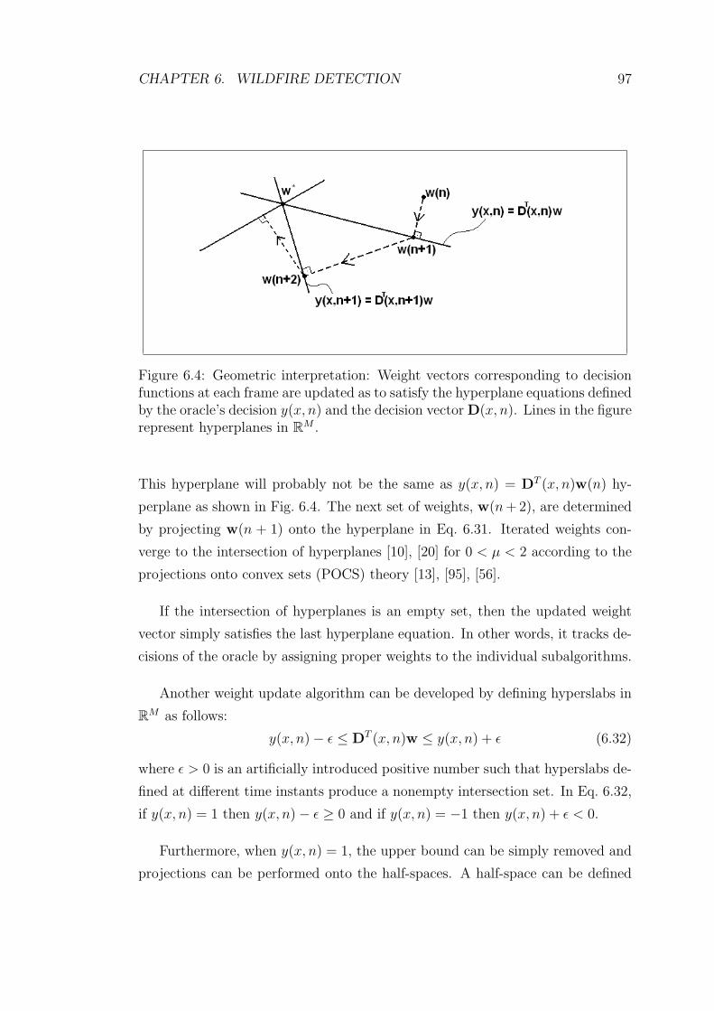
CHAPTER 6. WILDFIRE DETECTION 97
Figure 6.4: Geometric interpretation: Weight vectors corresponding to decisionfunctions at each frame are updated as to satisfy the hyperplane equations definedby the oracle’s decision y(x, n) and the decision vector D(x, n). Lines in the figurerepresent hyperplanes in RM .
This hyperplane will probably not be the same as y(x, n) = DT (x, n)w(n) hy-
perplane as shown in Fig. 6.4. The next set of weights, w(n + 2), are determined
by projecting w(n + 1) onto the hyperplane in Eq. 6.31. Iterated weights con-
verge to the intersection of hyperplanes [10], [20] for 0 < µ < 2 according to the
projections onto convex sets (POCS) theory [13], [95], [56].
If the intersection of hyperplanes is an empty set, then the updated weight
vector simply satisfies the last hyperplane equation. In other words, it tracks de-
cisions of the oracle by assigning proper weights to the individual subalgorithms.
Another weight update algorithm can be developed by defining hyperslabs in
RM as follows:
y(x, n)− ε ≤ DT (x, n)w ≤ y(x, n) + ε (6.32)
where ε > 0 is an artificially introduced positive number such that hyperslabs de-
fined at different time instants produce a nonempty intersection set. In Eq. 6.32,
if y(x, n) = 1 then y(x, n)− ε ≥ 0 and if y(x, n) = −1 then y(x, n) + ε < 0.
Furthermore, when y(x, n) = 1, the upper bound can be simply removed and
projections can be performed onto the half-spaces. A half-space can be defined

CHAPTER 6. WILDFIRE DETECTION 98
as follows:
DT (x, n)w ≥ 0 (6.33)
In other words, weighted combination of decision values of sub-algorithms must
be greater than 0, because the oracle states that y(x, n) = 1.
Weights, wi(n) ≥ 0, are kept non-negative in the weight update step to detect
smoke. Each wi(n) ≥ 0 corresponds to a half-space which are closed and convex.
Therefore, the POCS theory can be applied to this case as well. Whenever a
weight happens to be negative, its projection onto the half-space wi(n) ≥ 0 is
taken as 0.
For y(x, n) = −1, we have
DT (x, n)w < 0 (6.34)
In this case, the weight update equation for y(x, n) = 1 will be
w(n + 1) =
{w(n), if DT (x, n)w > 0
w(n) + µ e(x,n)||D(x,n)||2D(x, n), otherwise
(6.35)
where e(x, n) = Γ−DT (x, n)w(n) and Γ is any positive number. With this choice,
w(n + 1) satisfies DT (x, n)w(n + 1) > 0 (for Γ = 0, the weights correspond to
projection onto the hyperplane DT (x, n)w(n + 1) = 0).
For y(x, n) = −1, the weight update equation will be
w(n + 1) =
{w(n), if DT (x, n)w < 0
w(n) + µ e(x,n)||D(x,n)||2D(x, n), otherwise
(6.36)
where e(x, n) = Υ−DT (x, n)w(n) and Υ is any positive number.
It is almost impossible to know whether hyperplanes have a nonempty inter-
section set for this computer vision application. However, half-spaces defined by
Eqs. 6.33 and 6.34 and they probably have a nonempty intersection set. As a
result, weight updates do not diverge [95].
This set theoretic framework with tracking capability is especially useful
when the on-line active learning problem is of dynamic nature with drifting con-
cepts [72]. In this problem, the nature of forestal recordings vary over time due
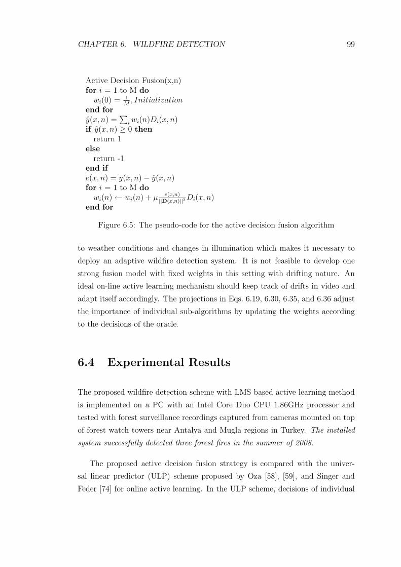
CHAPTER 6. WILDFIRE DETECTION 99
Active Decision Fusion(x,n)for i = 1 to M do
wi(0) = 1M
, Initializationend fory(x, n) =
∑i wi(n)Di(x, n)
if y(x, n) ≥ 0 thenreturn 1
elsereturn -1
end ife(x, n) = y(x, n)− y(x, n)for i = 1 to M do
wi(n) ← wi(n) + µ e(x,n)||D(x,n)||2 Di(x, n)
end for
Figure 6.5: The pseudo-code for the active decision fusion algorithm
to weather conditions and changes in illumination which makes it necessary to
deploy an adaptive wildfire detection system. It is not feasible to develop one
strong fusion model with fixed weights in this setting with drifting nature. An
ideal on-line active learning mechanism should keep track of drifts in video and
adapt itself accordingly. The projections in Eqs. 6.19, 6.30, 6.35, and 6.36 adjust
the importance of individual sub-algorithms by updating the weights according
to the decisions of the oracle.
6.4 Experimental Results
The proposed wildfire detection scheme with LMS based active learning method
is implemented on a PC with an Intel Core Duo CPU 1.86GHz processor and
tested with forest surveillance recordings captured from cameras mounted on top
of forest watch towers near Antalya and Mugla regions in Turkey. The installed
system successfully detected three forest fires in the summer of 2008.
The proposed active decision fusion strategy is compared with the univer-
sal linear predictor (ULP) scheme proposed by Oza [58], [59], and Singer and
Feder [74] for online active learning. In the ULP scheme, decisions of individual

CHAPTER 6. WILDFIRE DETECTION 100
Universal Predictor(x,n)for i = 1 to M do
wi(0) = 1M
, Initializationend foryu(x, n) =
∑i vi(n)Di(x, n)
if yu(x, n) ≥ 0 thenreturn 1
elsereturn -1
end iffor i = 1 to M do
vi(n + 1) =exp(− 1
2c`(y(x,n),Di(x,n)))∑
j exp(− 12c
`(y(x,n),Dj(x,n)))
`(y(x, n), Di(x, n)) = [y(x, n)−Di(x, n)]2
end for
Figure 6.6: The pseudo-code for the universal predictor
algorithms are linearly combined similar to Eq. 6.9 as follows:
yu(x, n) =∑
i
vi(n)Di(x, n) (6.37)
where the weights, vi(n), are updated according to the ULP algorithm, which
assumes that the data (or confidence values Di(x, n), in our case) is governed by
some unknown probabilistic model P [74]. The objective of a universal predictor is
to minimize the expected cumulative loss. An explicit description of the weights,
vi(n), of the ULP algorithm is given as follows:
vi(n + 1) =exp(− 1
2c`(y(x, n), Di(x, n)))∑
j exp(− 12c
`(y(x, n), Dj(x, n)))(6.38)
where c is a normalization constant and the loss function for the i-th decision
function is:
`(y(x, n), Di(x, n)) = [y(x, n)−Di(x, n)]2 (6.39)
The constant c is taken as 4 as indicated in [74]. The universal predictor based
algorithm is summarized in Fig. 6.6.
We also implemented the Weighted Majority Algorithm (WMA) as the de-
cision fusion step [47]. The WMA is summarized in Fig. 6.7 [58]. In WMA,
as opposed to our method, individual decision values from sub-algorithms are

CHAPTER 6. WILDFIRE DETECTION 101
Weighted Majority(x,n)for i = 1 to M do
wi(0) = 1M
, Initializationend forif
∑i:di(x,n)=1 wi(n) ≥ ∑
i:di(x,n)=−1 wi(n) thenreturn 1
elsereturn -1
end iffor i = 1 to M do
if di(x, n) 6= y then
wi(n + 1) ← wi(n)2
end ifend for
Figure 6.7: The pseudo-code for the Weighted Majority Algorithm
binary, i.e., di(x, n) ∈ {−1, 1}, which are simply the quantized version of real val-
ued Di(x, n) defined in Section 6.2. In the WMA, the weights of sub-algorithms
yielding contradictory decisions with that of the oracle are reduced by a factor of
two in an un-controlled manner, unlike the proposed LMS based algorithm and
the ULP scheme. Initial weights for WMA are taken as 1M
, as in the proposed
LMS based scheme.
The LMS based scheme, the ULP based scheme, the WMA based scheme, and
the non-adaptive approach with fixed weights are compared with each other in
the following experiments. In Tables 6.1 and 6.2, 6-hour-long forest surveillance
recordings containing actual forest fires and test fires as well as video sequences
with no fires are used.
We have 7 actual forest fire videos and 5 test fire videos ranging from 2 km
to 8 km captured in Antalya and Mugla regions in Turkey, in the summers of
2007 and 2008. All of the above mentioned decision fusion methods detect forest
fires within 8 seconds, as shown in Table 6.1. The detection rates of the methods
are comparable to each other. On the other hand, the proposed adaptive fusion
strategy significantly reduces the false alarm rate of the system by integrating the
feedback from the guard (oracle) into the decision mechanism within the active
learning framework described in Section 6.3. In Fig. 6.8 a typical false alarm
CHAPTER 6. WILDFIRE DETECTION 102
issued for shadows of clouds by an untrained algorithm with decision weights
equal to 14
is presented as a sequence of snapshots taken at seconds 1, 7, 13 and
18 from the clip V 15. The proposed algorithm does not produce a false alarm in
this video.
When a false alarm is issued by the compound algorithm, the learning process
is much faster for the LMS based scheme in comparison to the ULP and WMA
based methods. This is reflected in Fig. 6.9, in which the average squared error
functions ELMS(n), EULP (n) and EWMA(n) at image frame n, for the LMS, ULP
and the WMA based methods are shown, respectively. The average squared error
values are computed over all x in the image frame n, and defined as:
E(n) =1
NI
∑x
(e(x, n))2 (6.40)
where NI is the total number of pixels in the image frame, e(x, n) = y(x, n)− y(x, n)
and y(x, n) =∑
i wi Di(x, n). The average squared error values ELMS(n),
EULP (n) and EWMA(n) are computed after the first false alarm is issued. The
average squared error value ELMS(n) corresponding to the LMS based scheme
decays fast reaching around 0 within 5 frames of video which is about 1 sec. It
takes about 3 sec and 6 sec for the average squared error values EULP (n) and
EWMA(n) corresponding to the ULP and the WMA based schemes to converge.
The proposed LMS based method produces the lowest number of false alarms
in our data set. A set of video clips containing moving cloud shadows is used to
generate Table 6.2. These video clips are especially selected. Number of image
frames in which false alarms are issued by different methods are presented in
Table 6.2. Total number of false alarms for the clips in Table 6.2 issued by the
methods (a) the LMS based scheme, (b) the ULP based scheme, (c) the WMA
based scheme and (d) the non-adaptive approach with fixed weights are 5, 93,
240 and 612, respectively.
The software is currently being used in 10 forest watch towers in Antalya and
Mugla regions. We tested the system live and monitored the number of false
alarms for two days in September 2008. The current system produces 0.25 false
alarms per hour. This is an acceptable rate for a look-out tower.

CHAPTER 6. WILDFIRE DETECTION 103
Figure 6.8: Sequence of frames excerpted from clip V 15. Within 18 secondsof time, cloud shadows cover forestal area which results in a false alarm in anuntrained algorithm with decision weights equal to 1
4depicted as a bounding box.
The proposed algorithm does not produce a false alarm in this video.

CHAPTER 6. WILDFIRE DETECTION 104
Table 6.1: Frame numbers at which an alarm is issued with different methods forwildfire smoke captured at various ranges and fps. It is assumed that the smokestarts at frame 0.
Video Range Capture Frame number at which an alarm is issuedSequence (km) Frame Rate LMS Universal WMA Fixed
(fps) Based Based WeightsV1 4 7 24 22 28 20V2 8 7 44 48 40 51V3 2 7 28 35 38 29V4 3 5 33 38 26 37V5 5 10 58 67 69 41V6 6 10 40 41 38 32V7 6 10 38 36 30 35V8 6 10 53 57 56 47V9 6 10 67 71 56 71V10 3 5 28 34 32 35V11 5 7 42 40 36 39V12 5 7 51 55 54 44
6.5 Summary
An automatic wildfire detection algorithm using an LMS based active learning ca-
pability is developed. The compound algorithm comprises of four sub-algorithms
yielding their own decisions as confidence values in the range [−1, 1] ∈ R. The
LMS based adaptive decision fusion strategy takes into account the feedback from
guards of forest watch towers. Experimental results show that the learning du-
ration is decreased with the proposed online active learning scheme. It is also
observed that false alarm rate of the proposed LMS based method is the lowest in
our data set, compared to universal linear predictor (ULP) and weighted majority
algorithm (WMA) based schemes.
The tracking capability of the LMS algorithm is analyzed using a set theoretic
framework. The proposed framework for decision fusion is suitable for problems
with concept drift. At each stage of the LMS algorithm, the method tracks the
changes in the nature of the problem by performing an orthogonal projection
onto a hyperplane describing the decision of the oracle.

CHAPTER 6. WILDFIRE DETECTION 105
Table 6.2: The number of false alarms issued by different methods to video se-quences without any wildfire smoke.
Frame Video Number of framesVideo Rate Duration with false alarm
Sequence (fps) (sec.) LMS Universal WMA FixedBased Based Weights
V13 7 100 0 16 37 73V14 10 100 0 11 48 172V15 10 100 0 13 28 116V16 5 100 0 9 19 41V17 5 100 2 6 24 59V18 7 100 1 15 32 67V19 7 100 2 23 52 84
5 10 15 20 25 300
0.05
0.1
0.15
0.2
0.25
0.3
0.35
0.4
Frame Number
Avg
. Squ
ared
Err
or
UniversalLMSWMA
Figure 6.9: The average error curves for the LMS, universal predictor, and theWMA based adaptation algorithms in clip V 13. All of the algorithms convergeto the same average error value in this case, however the convergence rate ofthe LMS algorithm is faster than both the universal predictor and the WMAalgorithm.

Chapter 7
Conclusion and Future Work
Fire detection systems are vital in saving people’s lives, and preventing hazards
before they get out of control. Particle based detectors are commonly used in
such systems. These sensors are sensitive to produced during fire. An alarm
is issued only if these chemicals physically reach the sensor and their presence
is detected by either ionization or photometry. This requirement makes these
sensors dependent on the distance to fireplace as well as their location. Besides,
these sensors cannot be used outdoors. Image and video based systems can be
an alternative to particle sensors for fire detection.
In this thesis, we developed novel signal and image analysis techniques for au-
tomatic fire detection using cameras and infra-red sensors. Fire detection problem
can be also viewed as a problem of recognition of a specific dynamic texture type
in video. Dynamic texture and flame and smoke behavior can be modeled using
stochastic methods. In this thesis, we used Markov models which are tailored for
flame and smoke detection. We developed specific methods for flame, smoke and
wildfire smoke which have various spatio-temporal characteristics.
We developed dedicated methods for various aspects of fire using different
types of sensors. We explicitly developed real-time methods for
- short-range (< 30m) flame detection in visible range video,
106
CHAPTER 7. CONCLUSION AND FUTURE WORK 107
- short-range (< 30m) flame detection in long-wave infra-red (LWIR) video,
- short-range smoke detection in visible range video,
- short-range flame detection using pyro-electric infra-red (PIR) sensor, and
- long-range (> 100m) smoke detection in visible range video.
Each type of sensor has its own advantages and disadvantages on visualizing
different aspects of fire. Flames are visible when viewed by visible and IR sensors.
Although flame flicker becomes hard to observe as distance to the location of fire
increases. As a result, methods for short-range flame detection by IR and visible
sensors are proposed. Gradual increase in temperature can be monitored with IR
cameras and PIR sensors which can be helpful to take precautions even before
a fire starts. However, smoke, which is an early indicator of smoldering fires, is
transparent for LWIR cameras and PIR sensors. Consequently, smoke detection is
not possible using IR sensors. Smoke detection, both short and long-range, is only
possible with visible range cameras. Since long-range smoke has different spatio-
temporal characteristics than nearby smoke, separate algorithms are developed
for each case.
One common novelty that is introduced in all of the methods developed for
fire detection using several types of sensors is that flicker process in fire is charac-
terized using Markov models trained with wavelet based feature signals. Flicker
was not thoroughly characterized by previous studies on video based fire detec-
tion, which resulted in higher false alarm rates. Flicker modeling in a Markovian
setting suits well with the stochastic nature of fire. Besides, sub-band analysis (or
wavelet analysis) extracts non-stationarity inherent in flames and smoke. The use
of wavelet transform based feature signals, leads to the development of computa-
tionally efficient algorithms that work in real-time running on a standard PC.
Another important contribution of the thesis is the introduction of a novel set
theoretic framework for decision fusion and on-line active learning. As described
throughout the thesis, all of the proposed algorithms are composed of several sub-
algorithms yielding their own decisions and confidence values about the observed

CHAPTER 7. CONCLUSION AND FUTURE WORK 108
phenomenon. In the last stage of each detection algorithm, individual decisions
from sub-algorithms are combined together to reach a final decision. A least-
mean-square (LMS) based active decision fusion strategy is proposed and this
framework is successfully applied in the decision fusion step of the long-range
wildfire detection method.
The LMS adaptive decision fusion framework takes into account the feedback
from an oracle (security-guard) whose decisions are taken as the ground-truth.
Individual sub-algorithm weights are updated in such a way that the final decision
tracks the classification results of the oracle at each time step. At each stage of
the LMS algorithm, the method tracks the changes in the nature of the problem
by performing an orthogonal projection onto a hyperplane describing the decision
of the oracle. Therefore, the proposed framework for decision fusion may provide
insight in problems with drifting concepts belonging to many other research areas
in machine learning applications including computer vision.
The proposed wildfire detection method is integrated into forest fire early
warning systems which are installed in ten forest watch towers in Turkey. Our
system successfully did not miss any smoke due to test fires. It also detected three
forest fires in their early stages in Antalya and Aksehir regions in the summer
of 2008. The system is developed to assist the guard in fire detection. The
Directorate of Forestry and Ministry of Environment and Forestry of Turkey will
install the system to other forestal areas under high risk of fire in upcoming years.
In this thesis, we developed signal and image processing algorithms for fire
detection dedicated to sensing modalities like visible range and LWIR cameras,
and PIR senors. In the proposed setting, just a single type of sensor is assumed
to monitor an area of interest for each sensing modality.
A natural future direction pertains to extending both the number and types
of sensors covering an indoor or an outdoor area of interest. This extension
requires the development of algorithms that efficiently extract useful information
from multitude of sensors and interpret them to reach a final decision. The same
analysis algorithms may be used for each sensor. However, overall decision can
be given by linearly combining sensor outputs that define confidence levels for

CHAPTER 7. CONCLUSION AND FUTURE WORK 109
each sensor. The proposed set theoretic framework can be used to actively adapt
individual sensor weights in accordance with the feedback from an oracle.

Bibliography
[1] B. Albers and A. Agrawal. Schlieren analysis of an oscillating gas-jet diffu-
sion. Combustion and Flame, 119:84–94, 1999.
[2] H. Ammann, R. Blaisdell, M. Lipsett, S. Stone, S. Therriault, J. W. P.
Jenkins, and K. Lynch. Wildfire smoke - A guide for public health officials,
http://depts.washington.edu/wildfire/pubhlthguidev.9.0.pdf, Ac-
cessed at December 2008.
[3] M. Bagci, Y. Yardimci, and A. Cetin. Moving object detection using adap-
tive subband decomposition and fractional lower order statistics in video
sequences. Signal Processing, pages 1941–1947, 2002.
[4] I. Bosch, S. Gomez, L. Vergara, and J. Moragues. Infrared image processing
and its application to forest fire surveillance. In Proceedings of the IEEE
Conference on Advanced Video and Signal Based Surveillance (AVSS), pages
283–288, 2007.
[5] J. A. Broadbent. Fundamental flame flicker monitoring for power plant
boilers. In Proceedings of the IEE Seminar on Advanced Sensors and Instru-
mentation Systems for Combustion Processes, pages 4/1–4/4, 2000.
[6] H. Bunke and T. C. (Eds.). HMMs Applications in Computer Vision. World
Scientific, 2001.
[7] F. Carter and N. Cross. Combustion monitoring using infrared array-based
detectors. Measurement Science and Technology, 14:1117–1122, 2003.
110

BIBLIOGRAPHY 111
[8] CAVIAR: Context Aware Vision using Image-based Active Recognition.
Test Case Scenarios - EC Funded CAVIAR project/IST 2001 37540,
http://homepages.inf.ed.ac.uk/rbf/caviar/, Accessed at December
2008.
[9] A. Cetin, M. Akhan, B. Toreyin, and A.Aksay. Characterization of motion
of moving objects in video. US Patent No. 20040223652, pending, 2004.
[10] A. Cetin and R. Ansari. Signal recovery from wavelet transform maxima.
IEEE Transactions on Signal Processing, 42:194–196, 1994.
[11] A. Cetin and R. Ansari. Signal recovery from wavelet transform maxima.
IEEE Transactions on Signal Processing, 42:194–196, 1994.
[12] A. Cetin and D. Chetverikov. Dynamic Texture Detection in
Video Showcase, Multimedia Understanding through Semantics and
Learning, EC Sponsored Network of Excellence, MUSCLE-NoE,
http://www.muscle-noe.org/content/view/145/64/, Accessed at
December 2008.
[13] E. Cetin. Reconstruction of Signals from Fourier Transform Samples. Signal
Processing, 16:129–148, 1989.
[14] D. Chamberlin and A. Rose. The flicker of luminous flames. In Proceed-
ings of the First International Symposium on Combustion. The Combustion
Institute, 1928.
[15] A. Chan and N. Vasconcelos. Layered dynamic textures. In Proceedings
of the Conference on Neural Information Processing Systems (NIPS), pages
203–210, December 2005.
[16] A. Chan and N. Vasconcelos. Modeling, clustering, and segmenting video
with mixtures of dynamic textures. IEEE Transactions on Pattern Analysis
and Machine Intelligence, 30(5):909–926, 2008.
[17] T. Chen, P. Wu, and Y. Chiou. An early fire-detection method based on
image processing. In Proceedings of the IEEE International Conference on
Image Processing (ICIP), pages 1707–1710, 2004.
BIBLIOGRAPHY 112
[18] D. Chetverikov and R. Peteri. A brief survey of dynamic texture description
and recognition. In Proceedings of the Fourth International Conference on
Computer Recognition Systems (CORES), pages 17–26, 2005.
[19] R. Collins, A. Lipton, and T. Kanade. A system for video surveillance and
monitoring. In Proceedings of the 8-th International Topical Meeting on
Robotics and Remote Systems. American Nuclear Society, April 1999.
[20] P. L. Combettes. The foundations of set theoretic estimation. Proceedings
of the IEEE, 81(2):182–208, 1993.
[21] J. Davis and A. Bobick. The representation and recognition of action using
temporal templates. In Proceedings of the IEEE Conference on Computer
Vision and Pattern Recognition (CVPR), pages 928–934, 1997.
[22] J. M. de Dios, B. Arrue, A. Ollero, L. Merino, and F. Gomez-Rodriguez.
Computer vision techniques for forest fire perception. Image and Vision
Computing, 26(4), 2008.
[23] Y. Dedeoglu, B. Toreyin, U. Gudukbay, and A. Cetin. Real-time fire and
flame detection in video. In Proceedings of the IEEE International Confer-
ence on Acoustics, Speech and Signal Processing (ICASSP), pages 669–672,
2005.
[24] Y. Dedeoglu, B. Toreyin, U. Gudukbay, and A. Cetin. Multimodal Processing
and Interaction: Audio, Video, and Text, chapter 6 - Surveillance Using Both
Video and Audio, pages 143–155. P. Maragos, A. Potamianos, P. Gros. (Eds.)
Springer Science+Business Media, LLC, 2008.
[25] H. Dreyfus. What Computers Can’t Do. 1972.
[26] H. Dreyfus. What Computers Still Can’t Do: A Critique of Artificial Reason.
MIT Press, 1992.
[27] R. O. Duda, P. E. Hart, and D. G. Stork. Pattern Classification. Wiley-
Interscience Publication, 2000.

BIBLIOGRAPHY 113
[28] R. Fablet and P. Bouthemy. Motion recognition using nonparametric im-
age motion models estimated from temporal and multiscale co-occurrence
statistics. IEEE Transactions on Pattern Analysis and Machine Intelligence,
25:1619–1624, 2003.
[29] S. Fazekas and D. Chetverikov. Analysis and performance evaluation of op-
tical flow features for dynamic texture recognition. Signal Processing:Image
Communication, 22(7-8):680–691, 2007.
[30] R. Fisher (Ed.). CVonline: The Evolving, Distributed, Non-
Proprietary, On-Line Compendium of Computer Vision,
http://homepages.inf.ed.ac.uk/rbf/cvonline/, Accessed at December
2008.
[31] G. L. Foresti, C. S. Regazzoni, and P. K. V. (Eds.). Multisensor Surveillance
Systems - The Fusion Perspective. Kluwer Academic Publishers, 2003.
[32] D. Forsyth and J.Ponce. Computer Vision: A Modern Approach. Prentice
Hall, 2002.
[33] K. Fujita and S. Nayar. Recognition of dynamic textures using impulse
responses of state variables. In Proceedings of the Third International Work-
shop on Texture Analysis and Synthesis (Texture), pages 31–36, 2003.
[34] O. N. Gerek and A. E. Cetin. Adaptive polyphase subband decomposition
structures for image compression. IEEE Transactions on Image Processing,
9:1649–1659, October 2000.
[35] A. Ghoreyshi and R. Vidal. Segmenting Dynamic Textures with Ising De-
scriptors, ARX Models and Level Sets. In Proceedings of the European Con-
ference on Computer Vision / Dynamical Vision Workshop (ECCV/DV),
2006.
[36] P. Guillemant and J. Vicente. Real-time identification of smoke images by
clustering motions on a fractal curve with a temporal embedding method.
Optical Engineering, 40:554–563, 2001.
[37] S. Haykin. Adaptive Filter Theory. Prentice Hall, 2002.

BIBLIOGRAPHY 114
[38] G. Healey, D. Slater, T. Lin, B. Drda, and A. Goedeke. A system for real-
time fire detection. In Proceedings of the IEEE Conference on Computer
Vision and Pattern Recognition (CVPR), pages 15–17, 1993.
[39] M. Hefeeda and M. Bagheri. Wireless sensor networks for early detection
of forest fires. In Proceedings of the International Workshop on Mobile Ad
hoc and Sensor Systems for Global and Homeland Security (MASS-GHS),
October 2007.
[40] F. Heijden. Image Based Measurement Systems: Object Recognition and
Parameter Estimation. Wiley, 1996.
[41] T. Horprasert, D. Harwood, and L. Davis. A statistical approach for real-
time robust background subtraction and shadow detection. In Proceedings
of the IEEE International Conference on Computer Vision/FRAME-RATE
Workshop (CVPR/FR), 1999.
[42] H. Huang, Y. Yan, G. Lu, and A. Reed. On-line flicker measurement of
gaseous flames by imaging processing and spectral analysis. Measurement
Science and Technology, 10:726–733, 1999.
[43] O. Javed and M. Shah. Tracking and object classification for automated
surveillance. In Proceedings of the European Conference on Computer Vision
(ECCV), pages 343–357, 2002.
[44] S. Khare and S. Negi. Thermal (infrared) imaging sensors. Defence Science
Journal, 57(3):173–183, 2007.
[45] C. Kim, R. Ansari, and A. Cetin. A class of linear-phase regular biorthogonal
wavelets. In Proceedings of the IEEE International Conference on Acoustics,
Speech and Signal Processing (ICASSP), pages 673–676, 1992.
[46] J. Li, Q. Qi, X. Zou, H. Peng, L. Jiang, and Y. Liang. Technique for auto-
matic forest fire surveillance using visible light image. In Proceedings of the
International Geoscience and Remote Sensing Symposium, volume 5, pages
31–35, 2005.

BIBLIOGRAPHY 115
[47] N. Littlestone and M. Warmuth. The weighted majority algorithm. Infor-
mation and Computation, 108:212261, 1994.
[48] C. Liu and N. Ahuja. Vision based fire detection. In Proceedings of the
International Conference on Pattern Recognition (ICPR), volume 4, 2004.
[49] C.-B. Liu, R.-S. Lin, and N. Ahuja. Modeling dynamic textures using sub-
space mixtures. In Proceedings of the IEEE International Conference on
Multimedia and Expo (ICME), 2005.
[50] C.-B. Liu, R.-S. Lin, N. Ahuja, and M.-H. Yang. Dynamic textures synthesis
as nonlinear manifold learning and traversing. In Proceedings of the 17th
British Machine Vision Conference (BMVC), pages 859–868, 2006.
[51] Z. Lu, W. Xie, J. Pei, and J. Huang. Dynamic texture recognition by spatio-
temporal multiresolution histogram. In Proceedings of the IEEE Workshop
on Motion and Video Computing (WACV/MOTION), volume 2, pages 241–
246, 2005.
[52] S. Mallat and S. Zhong. Characterization of signals from multiscale
edges. IEEE Transactions on Pattern Analysis and Machine Intelligence,
14(7):710–732, 1992.
[53] R. Q. N. Haering and M. Sezan. Approach and its application to detecting
hunts in wildlife video. IEEE Transactions on Circuits and Systems for
Video Technology, 10(6):857–868, 2000.
[54] M. Naphade, T. Kristjansson, B. Frey, and T. Huang. Multimedia Objects
(Multijects): A Novel Approach to Video Indexing and Retrieval in Mul-
timedia Systems. In Proceedings of the IEEE International Conference on
Image Processing (ICIP), pages 536–540, 1998.
[55] R. Nelson and R. Polana. Qualitative recognition of motion using temporal
texture. Computer Vision, Graphics and Image Processing (CVGIP): Image
Understanding, 56:78–89, July 1992.

BIBLIOGRAPHY 116
[56] U. Niesen, D. Shah, and G. Wornell. Adaptive alternating minimization algo-
rithms. In Proceedings of the IEEE International Symposium on Information
Theory (ISIT), pages 1641–1645, June 2007.
[57] K. Otsuka, T. Horikoshi, S. Suzuki, and M. Fujii. Feature extraction of
temporal texture based on spatiotemporal motion trajectory. In Proceedings
of the International Conference on Pattern Recognition (ICPR), volume 2,
pages 1047–1051, 1998.
[58] N. Oza. Online Ensemble Learning. PhD thesis, Electrical Engineering and
Computer Sciences, University of California, September 2001.
[59] N. Oza. Online bagging and boosting. In Proceedings of the IEEE In-
ternational Conference on Systems, Man and Cybernetics, volume 3, pages
2340–2345, October 2005.
[60] B. Parhami. Voting algorithms. IEEE Transactions on Reliability, 43(4):617–
629, 1994.
[61] T. Pavlidis. Computers versus Humans, http://www.theopavlidis.com/
comphumans/comphuman.htm, Accessed at December 2008.
[62] C. Peh and L.-F. Cheong. Synergizing spatial and temporal texture. IEEE
Transactions on Image Processing, 11:11791191, 2002.
[63] R. Peteri, M. Huiskes, and S. Fazekas. DynTex-A comprehensive database of
Dynamic Textures http://old-www.cwi.nl/projects/dyntex/, Accessed
at December 2008.
[64] W. Phillips, M. Shah, and N. Lobo. Flame recognition in video. Pattern
Recognition Letters, 23:319–327, 2002.
[65] F. Porikli, Y. Ivanov, and T. Haga. Robust abandoned object detection
using dual foregrounds. EURASIP Journal on Advances in Signal Processing,
2008(1):1–10, 2008.
[66] A. Prati, I. Mikic, M. Trivedi, and R. Cucchiara. Detecting moving shadows:
Algorithms and evaluation. IEEE Transactions on Pattern Analysis and
Machine Intelligence, 25:918923, 2003.

BIBLIOGRAPHY 117
[67] L. Rabiner and B.-H. Juang. Fundamentals of Speech Recognition. Prentice-
Hall Inc., 1993.
[68] A. Rahman and M. Murshed. Real-time temporal texture characterisation
using block-based motion co-occurrence statistics. In Proceedings of the
IEEE International Conference on Image Processing (ICIP), pages 1593–
1596, 2004.
[69] D. Reynolds and R. Rose. Robust text-independent speaker identification
using gaussian mixture speaker models. IEEE Transactions on Speech and
Audio Processing, 3(1):72–83, 1995.
[70] Y. Sahin. Animals as mobile biological sensors for forest fire detection. Sen-
sors, 7(12):3084–3099, 2007.
[71] P. Saisan, G. Doretto, Y. Wu, and S. Soatto. Dynamic texture recognition.
In Proceedings of the IEEE Conference on Computer Vision and Pattern
Recognition (CVPR), volume 2, pages 58–63, December 2001.
[72] J. Schlimmer and R. Granger. Incremental learning from noisy data. Machine
Learning, 1, page 317354, 1986.
[73] B. Schnaufer and W. Jenkins. New data-reusing LMS algorithms for im-
proved convergence. In Proceedings of the Asilomar Conference, Pacific
Groves, CA, pages 1584–1588, 1993.
[74] A. Singer and M. Feder. Universal linear prediction by model order weight-
ing. IEEE Transactions on Signal Processing, 47-10:2685–2699, 1999.
[75] J. Smith, C.-Y. Lin, and M. Naphade. Video texture indexing using spa-
tiotemporal wavelets. In Proceedings of the IEEE International Conference
on Image Processing (ICIP), volume 2, pages 437–440, 2002.
[76] L. St-Laurent, D. Prvost, and X. Maldague. Thermal imaging for enhanced
foreground-background segmentation. In Proceedings of the 8-th Interna-
tional Conference on Quantitative InfraRed Thermography, 2006.

BIBLIOGRAPHY 118
[77] C. Stauffer and W. Grimson. Adaptive background mixture models for real-
time tracking. In Proceedings of the IEEE Conference on Computer Vision
and Pattern Recognition (CVPR), volume 2, 1999.
[78] W. Straumann, D. Rizzotti, and N. Schibli. Method and Device for Detecting
Fires Based on Image Analysis. European Patent EP 1,364,351, 2002.
[79] M. Szummer and R. W. Picard. Temporal texture modeling. In Proceedings
of the IEEE International Conference on Image Processing (ICIP), volume 3,
pages 823–826, 1996.
[80] Y. Takatoshi. Fire Detecting Device. Japanese Patent 11,144,167, 1999.
[81] M. Thuillard. Method and Device for Detecting Fires Based on Image Anal-
ysis. US Patent 6,011,464, 1998.
[82] M. Thuillard. A new flame detector using the latest research on flames and
fuzzy-wavelet algorithms. Fire Safety Journal, 37:371–380, 2002.
[83] B. Toreyin. Moving object detection and tracking in wavelet compressed
video. Master’s thesis, Bilkent University, Department of Electrical and
Electronics Engineering, Ankara, Turkey, 2003.
[84] B. Toreyin, Y. Dedeoglu, and A. Cetin. Flame detection in video using
hidden markov models. In Proceedings of the IEEE International Conference
on Image Processing (ICIP), pages 1230–1233, 2005.
[85] B. Toreyin, Y. Dedeoglu, and A. Cetin. HMM Based Falling Person Detec-
tion Using Both Audio and Video. In Proceedings of the IEEE International
Workshop on Human-Computer Interaction (HCI), volume 3766, pages 211–
220, 2005.
[86] B. Toreyin, Y. Dedeoglu, and A. Cetin. Wavelet based real-time smoke
detection in video. In Proceedings of the 13-th European Signal Processing
Conference (EUSIPCO), 2005.
[87] B. Toreyin, Y. Dedeoglu, U. Gudukbay, and A. Cetin. Computer vision
based system for real-time fire and flame detection. Pattern Recognition
Letters, 27:49–58, 2006.

BIBLIOGRAPHY 119
[88] B. Toreyin, E. Soyer, I. Onaran, and A. Cetin. Falling person detection
using multi-sensor signal processing. EURASIP Journal on Advances in
Signal Processing, 2008(1):1–10, 2008.
[89] R. Vidal and A. Ravichandran. Optical flow estimation and segmentation of
multiple moving dynamic textures. In Proceedings of the IEEE Conference
on Computer Vision and Pattern Recognition (CVPR), volume 2, pages 516–
521, 2005.
[90] L.-Y. Wei and M. Levoy. Fast texture synthesis using tree-structured vec-
tor quantization. In Proceedings of the 27-th International Conference on
Computer Graphics and Interactive Techniques (ACM SIGGRAPH), pages
479–488, 2000.
[91] B. Widrow and M. Hoff. Adaptive switching circuits. In Proceedings of the
IRE WESCON (New York Convention Record), volume 4, pages 96–104,
1960.
[92] B. Widrow, J. McCool, M. Larimore, and C. Johnson. Stationary and non-
stationary learning characteristics of the LMS adaptive filter. Proceedings of
the IEEE, 64(8):1151–1162, 1976.
[93] B. Widrow and S. Stearns. Adaptive Signal Processing. Prentice Hall, 1985.
[94] Z. Xiong, R. Caballero, H. Wang, A. Finn, M. Lelic, and P.-
Y. Peng. Video based Smoke Detection: Possibilities, Tech-
niques, and Challenges, available at http://vision.ai.uiuc.edu/∼wanghc/papers/smoke_detection.pdf, Accessed at December 2008.
[95] D. Youla and H. Webb. Image restoration by the method of convex projec-
tions, Part I-Theory. IEEE Transactions on Medical Imaging, MI-I-2:81–94,
1982.
[96] J. Zhong and S. Sclaroff. Segmenting foreground objects from a dynamic
textured background via a robust kalman filter. In Proceedings of the Inter-
national Conference on Computer Vision (ICCV), pages 44–50, 2003.