fionn murtagh (1), adam ganz (2) and stewart mckie (2 ... · day, night. there is also dialog and...
TRANSCRIPT

The Structure of Narrative: the Case of Film
Scripts
Fionn Murtagh (1), Adam Ganz (2) and Stewart McKie (2)(1) Department of Computer Science
(2) Department of Media ArtsRoyal Holloway, University of London, Egham TW20 0EX, England
Contact author: fmurtagh at acm dot org
May 28, 2018
Abstract
We analyze the style and structure of story narrative using the case offilm scripts. The practical importance of this is noted, especially the needto have support tools for television movie writing. We use the Casablancafilm script, and scripts from six episodes of CSI (Crime Scene Investiga-tion). For analysis of style and structure, we quantify various central per-spectives discussed in McKee’s book, Story: Substance, Structure, Style,and the Principles of Screenwriting. Film scripts offer a useful point ofdeparture for exploration of the analysis of more general narratives. Ourmethodology, using Correspondence Analysis, and hierarchical clustering,is innovative in a range of areas that we discuss. In particular this work isgroundbreaking in taking the qualitative analysis of McKee and groundingthis analysis in a quantitative and algorithmic framework.
Kewwords: data mining, data analysis, factor analysis, correspondence anal-ysis, semantic space, Euclidean display, hierarchical clustering, narrative, story,film script
1 Introduction
As a framework for analysis of narrative in many areas of application, filmscripts have a great deal to offer. We present quite a number of innovations inthis work: quantifying and automating a range of qualitative ways of addressingpattern recognition in narrative; use of metric embedding using CorrespondenceAnalysis, and ultrametric embedding through hierarchical clustering of a datasequence, in order to capture semantics in the data; and verifying experimentallythe well foundedness of much that McKee [15] describes in qualitative terms.
Other than the data mining, two distinct levels of user are at issue here.Firstly and foremostly, we have the scriptwriter or screenwriter in mind. See
1
arX
iv:0
805.
3799
v1 [
cs.A
I] 2
4 M
ay 2
008

[15] for a content-based description of the scriptwriting process. Secondly andmore indirectly we have the movie viewer in mind. The feasibility of usingstatistical learning methods in order to map a characterization of film scripts(essentially using 22 characteristics) onto box office profitability was pursuedby [7]. The importance of such machine learning of what constitutes a goodquality and/or potentially profitable film script has been the basis for (success-ful) commercial initiatives, as described by [8]. The business side of the moviebusiness is elaborated on in some depth in terms of avenues to be explored inthe future, in [6].
A film script is semi-structured in that it is subdivided into scenes and some-times other structural units. Furthermore there is metadata provided relatedto location (internal, external; particular or general location name); characters;day, night. There is also dialog and description of action in free text.
There are literally thousands of film scripts, for all genres, available andopenly accessible (e.g. IMSDb, The Internet Movie Script Database, www.imsdb.com).While offering just one data modality, viz. text, there is close linkage to othermodalities, visual, speech and often music.
An area of application of our work that is of particular importance is tomovies for television. In contrast to a cinema movie, in television a serialdramatization is formulaic in its set of characters, their actions, location, andin content generally. In form it is even more formulaic, in length, initial scenes,positioning of advertisement breakpoints, and in other aspects of format. Whilescreenwriting and subsequent aspects of cinema movie creation and develop-ment have been much studied (e.g. [15]), film writing for television has been lessso. The latter is often team-based, and much more “managed” on account ofits linkages with other dramatizations in the same series, or in closely relatedseries. These properties of television serial dramatization lead, perhaps evenmore than for cinema movie, to a need for tools to quantitatively support scriptwriting.
Film scripts constitute an outstanding template or model for other domains.One longer term goal of our work is for our tools to provide a platform for in-troducing interactivity into a movie. Interactivity with a film or video includesthe following possible uses: (i) it provides an approach to developing interac-tive games; (ii) it allows for use in interactive and even immersive training andlearning environments; and (iii) support is also feasible for use in the enter-tainment area, e.g. interactive television. Leveraging the existing corpus and“fanbase” of hit scripts to create new interactive versions could create a wholenew sector of movie script based interactive games or filmed variant-sequels tofamous movies that take the familiar in a different direction. The convergenceof story-telling and narrative, on the one hand, and games, on the other, isexplored in [9]. There and in [20], story graphs and narrative trees are used as away to open up to the user the range of branching possibilities available in thestory. A further longer term goal lies in the area of business analysis, especiallyin distributed, video-conferencing and other, settings. The narrative structure,similar to a film script, gives the analyst the framework for generating stories.Such narrative structures can be used for analysis of meetings, projects, dialogs,
2

and any interactive sessions in real or virtual meetings.Our work is hugely topical. A television serial episode costs between $2
to $3 million for one hour of television. New series are scripted and run ontelevision channels and only then is viewer reaction used to determine theirviability. This points to major potential savings. Understanding and supportingscriptwriting is crucial. An additional motivation is that the entertainment andcultural market is moving towards greater interactivity, and our work is of greatpotential here too.
The structure of the paper is as follows. In section 2, we provide essen-tial background on the analysis approach taken. In section 3, we discuss theplausibility of taking text as a proxy for, or a practical and useful expression of,underlying content that we refer to as the story. In section 4, we describe brieflythe data analysis algorithms that we use, providing citations to more detailedbackground reading.
In section 5 we study a number of aspects of the Casablanca movie script.In section 6, we turn attention to the television series, CSI (Crime Scene Inves-tigation, Las Vegas).
Among important aspects of this work are the following. Firstly, we recasta number of issues discussed by McKee [15] in a quantitative and algorithmicform. Secondly, we employ Correspondence Analysis as a versatile data analy-sis framework. Since in Correspondence Analysis, each scene is expressed as anaverage of attributes used to characterize the scenes, and since each attribute isexpressed as an average of the scenes they characterize, we have in Correspon-dence Analysis a way to represent and study semantics. Thirdly, our clusteringof film script units (e.g., scenes) is innovative in a few ways, including respectingthe sequence of film script units, and taking as input the “direction” of the filmscript content rather than having a more static framework for the input (whichwe found empirically to work less well in that it was far less discriminatory).This type of clustering captures the semantics of change. If scenes are verydissimilar they will be agglomerated late in the sequence of agglomerations.
2 Analysis of Change in Content Over Time
Analysis of a film script has everything to do with change in the course of thestory, as we will now discuss, following McKee [15]. “The finest writing ... arcsor changes ... over the course of the telling” (p. 104, [15]).
A typical film has 40 to 60 “story events” or scenes. A scene is a storyin miniature and must have activity or change. A scene will typically (with,of necessity, large variability) translate into 2 to 3 minutes of film. In ourwork we have examples of very short (one or two sentence) dialog or actiondescriptions in scenes. Compared to longer scenes, such short scenes can beequally revealing and significant. Units of action or behavior within a scene aretermed beats by McKee. We will examine beats below in a case study using theCasablanca script. Ideally every scene is a turning point, in character behavior,or in changing the “values” involved from positive to negative or vice versa.
3
Moving upwards now in scale of units of film script, a sequence is a seriesof typically 2 to 5 scenes. A sequence expresses significant albeit moderatechange. An act is a set of sequences expressing major impact. Acts are the“macro-structure of story” (p. 217, [15]). It is possible to have a one-act playor story, although this would be quite unusual.
The overall set of scenes (or sequences, or acts) is termed the plot. A climaxin a sequence or act or plot is essential. It is final and irreversible (pp. 41–42,[15]). It is possible to distinguish between an open and a closed ending, respec-tively bringing finality versus leaving some issues hanging, and this does notalter the all-important climax. A sequence climax is of moderate importance,an act climax is of greater importance, and the plot climax is crucial. In thisscheme of things, each scene is a turning point of limited, moderate or greatimportance in the context of the overall plot or story.
The degree of change is the difference between a scene and the scene thatclimaxes a sequence, or the scene that climaxes an act, or the overall and globalclimax of the plot. In the plot, there is no room for a missing scene, or asuperfluous scene, or a misordering of scenes.
Rhythm and tempo are related to scene length. The former, rhythm, shouldbe very variable in order to keep the viewer’s (reader’s) attention, allowingfor a soft upper limit on the time-span of attention. Tempo can exemplifyclimax in two ways: firstly, through increasingly shortened scenes (or otherunits) leading up to a climax; and, secondly, through the climax being of clearlygreater length than the preceding scene (in order to allow for sufficient timeto elaborate and offload its content). A decrease in tempo, through a suddenincrease in scene length, can be indicative of denouement and climax. Increasingtempo, manifested through successively decreasing scene length, expresses abuild-up of tension.
Our discussion up to now has been about story. We turn to types of struc-ture. McKee [15] categorizes design into classical; minimalist or miniplot; andanti-structure or antiplot. In this categorization scheme for film, the minimalistdesign dovetails very well with television film and drama, with e.g. open ending,unreconciled internal conflict, and passive and/or multiple protagonists. Belowwe will explore case studies based on episodes of CSI (Crime Scene Investiga-tion).
3 Justification for Textual Analysis of Film Script
In this section we address the issue of plausibility of appreciable analysis ofcontent based on what are ultimately the statistical frequencies of co-occurrenceof words.
Words are a means or a medium for getting at the substance and energyof a story (p. 179, [15]). Ultimately sets of phrases express such underlyingissues (the “subtext”, as expressed by McKee, a term we avoid due to possibleconfusion with subsets of text) as conflict or emotional connotation (p. 258).We have already noted that change and evolution is inherent to a plot. Human
4
emotion is based on particular transitions. So this establishes well the possibil-ity that words and phrases are not taken literally but instead can appropriatelycapture and represent such transition. Text, says McKee, is the “sensory sur-face” of a work of art (counterposing it to the subtext, or underlying emotionor perception).
Simple words can express complex underlying reality. Aristotle, for example,used words in common usage to express technically loaded concepts ([18], p.169), and Freud did also.
Best practice in film script writing includes the following. Present tensedominates all ([15], p. 395): “The ontology of the screen is an absolute presenttense in constant vivid movement” (emphasis in original). Clipped diction isneeded. Generic nouns are avoided in favor of specific terms, and similarlyadjectives and adverbs are to be avoided. The verb “to be” is to be avoidedbecause: “Onscreen nothing is in a state of being; story life is an unendingflux of change, of becoming” (p. 396). Simile and metaphor are out, as is anyexplicit positioning of context on behalf of the reader of the script or viewer ofthe film.
4 Methodology: Euclidean Embedding throughCorrespondence Analysis, and Clustering theSuccession of Film Script Scenes
We have already noted (section 1) some novel aspects of our methodology. Webegin with the display of data (e.g., scenes and/or words) where visualization ofrelationships is greatly facilitated by having a Euclidean embedding. We showhow Correspondence Analysis furnishes such a metric space embedding of theinformation present in the film script text, and furthermore how this facilitatesan ultrametric (i.e. hierarchical) embedding that takes account of the temporal,semantic dynamic of the film script narrative.
4.1 A Note on Correspondence Analysis
Correspondence Analysis [18] takes input data in the form of frequencies ofoccurrence, or counts, and other forms of data, and produces such a Euclideanembedding. The Appendix provides a short introduction to CorrespondenceAnalysis and hierarchical clustering.
We start with a cross-tabulation of a set of observations and a set of at-tributes. This starting point is an array of counts of presence versus absence, orfrequency of occurrence. From this input data, we can embed the observationsand attributes in a Euclidean space. This factor space is mathematically opti-mal in a certain sense (using the least squares criterion, which is also Huyghens’principle of decomposition of inertia). Furthermore a Euclidean space allows foreasy visualization that would be more awkward to arrange otherwise.
5

A third reason for the particular embedding used for the observations andattributes in the Euclidean factor space is that weighting of observations andattributes is handled naturally in this framework. The issue of weighting has tobe addressed somehow, with one option being to treat the set (of observationsor of attributes) as identically weighted, and hence of equal a priori importance.Very often either observations or attributes follow a power law: examples of suchpower laws include Zipf’s law (in natural language texts, the word frequency isinversely proportional to its rank), the Pareto distribution in economics, andmany others [19]. Correspondence Analysis handles weighting of observationsand attributes at the “core” of its algorithm [18].
Application of the power law property to social networks has included thenetwork of movie actors [19]. As counterposed to such work, our interest is inanalyzing a time series of data. The succession of scenes in a movie, or acts ina play, exemplify this.
4.2 Input Data Used
We take all words into account in the semi-structured texts that are providedby film (or television program) scripts. Punctuation is ignored. Upper case isconverted to lower case for our purposes. Words must be at least two charactersin length. Any numerical figure, or term beginning with a numerical, is ignored.We have already noted above (section 3; see also the case studies and discussionin [18]) why the use of all words in this way is, in principle, feasible and justified.
Occurrences or presence/absence data therefore are the point of departure.Each scene is cross-tabulated by the set of all words so that, in this cross-tabulation table, at the intersection of scene i and word j we have a presence (1)or absence (0) value. To employ notions of change or proximity between scenes,we need this data to be appropriately represented in a numerically well-definedsemantic space. This is provided by mapping the frequencies of occurrence datainto a Euclidean space, using Correspondence Analysis.
4.3 Hierarchical Agglomerative Clustering Respecting Se-quence
Unusually in this work, we use hierarchical clustering taking a sequence of filmscript units (e.g., scenes) into account. Our motivation is the following: largeultrametric or tree distances derived from the hierarchy have a ready interpre-tation in terms of change. A brief introduction is provided in the Appendix. Ashort discussion follows.
Hierarchical clustering is carried out through a sequence of agglomerationsof successive scenes or of clusters (or temporal segments or intervals) of suc-cessive scenes. Respect for the sequentiality of the scenes is ensured throughthe requirement that agglomerands must be adjacent. In addition to this, theleast dissimilar scenes are checked, with the criterion being: merge two clusterswhen the greatest dissimilarity between cluster members (scenes) is minimal.The least dissimilar pair of scenes, considering two potential agglomerands, is
6

what we use as our agglomeration criterion. This is the contiguity-constrainedcomplete link hierarchical clustering method. Apart from heuristic reasons forfavoring it, it has some further properties that will now be discussed briefly.
The sequence-related adjacency requirement must take into considerationwhether an agglomerative clustering method would give rise to an inversion,i.e., a later agglomeration in the sequence of agglomerations would have an as-sociated criterion value that is less than the previous criterion value. It is nothard to appreciate that our desire to have gradations of distance represented bythe dendrogram would be negated, and severely so, by such absence of the mono-tonicity of criterion value, which amounts to a contradiction in interpretationof the dendrogram.
It is shown in [17] that two algorithms are feasible. What is involved here issketched out as follows.
Continuity-constrained single link hierarchical clustering is simultaneouslyhierarchical clustering on the spanning graph. This is easy to implement (in-efficiently): just fix an infinite (or very large) distance between non-contiguouspairs and proceed to use single link hierarchical clustering [17].
The complete link method, with the constraint that at least one member ofeach of the two clusters to be agglomerated be contiguous, is guaranteed not togive rise to inversions. The O(n2) time, O(n2) space algorithm for the completelink method, based on the nearest neighbor chain (see [17]), is easily modifiedto include an additional testing of contiguity whenever a linkage in the nearestneighbor chain is created.
In this work we use the latter, in view of the well-balanced hierarchies typi-cally produced, [16].
5 Casablanca Film Script Analysis
5.1 Data Used
Based on the unpublished 1940 screenplay by Murray Burnett and Joan Al-lison, [3], the Casablanca script by Julius J. Epstein, Philip G. Epstein andHoward Koch led to the film directed by Michael Curtiz, produced by Hal B.Wallis and Jack L. Warner, and shot by Warner Bros. between May and August1942. We used the script from The Internet Movie Script Database, IMSDb(www.imsdb.com).
The Casablanca film script comprises 77 successive scenes. All told, therewere 6710 words in these successive scenes.
The source text for the 77 scenes, including metadata, varied between just 5words, and 1017 words (scene 22). Typical Zipf distributional behavior is seenin the marginals. All words were used, following the imposing of lower casethroughout. This was subject only to words being longer than one character.No stemming or other preprocessing was used. The top word frequencies wereinteresting: the, 965; rick, 689; you, 651; to, 574; and, 435; in, 332; of, 319;renault, 284; it, 271; ilsa, 256; laszlo, 255; he, 236; is, 232; at, 192; that, 171; for,
7

158; we, 151; on, 149; strasser, 135. The numerically high presence of personalnames is quite unusual relative to more general texts, and characterizes this filmscript text. A major reason for this is that character names head up each dialogblock.
Casablanca is based on a range of miniplots. This occasions considerablevariety. Miniplots include: love story, political drama, action sequences, urbanedrama, and aspects of a musical. The composition of Casablanca is said byMcKee [15] to be “virtually perfect” (p. 287).
5.2 Analysis of Casablanca’s “Mid-Act Climax”, Scene 43
To illustrate our methodology, applied below to scenes, we look first in depthat one particular scene.
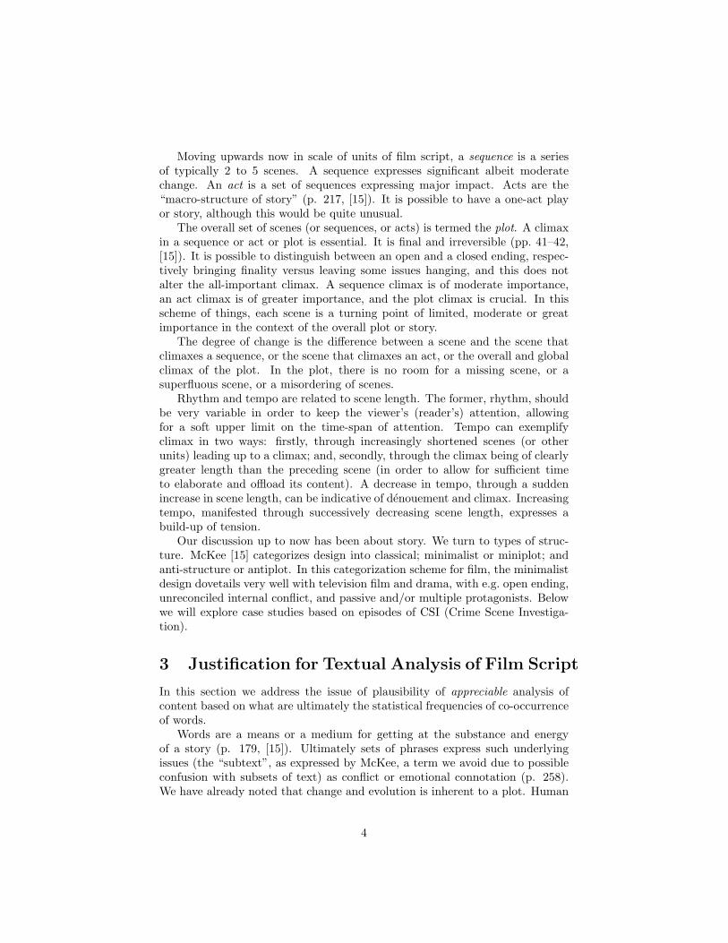
This scene is discussed in detail in McKee [15], who subdivides it into 11successive beats (here understood as subscenes). It relates to Ilsa and Rickseeking black market exit visas. Beat 1 is Rick finding Ilsa in the market. Beats2, 3 and 4 are rejections of him by Ilsa. Beats 5 and 6 express rapprochementby both characters. Beat 7 is guilt-tripping by each in turn. Beat 8 is a jumpin content: Ilsa says she will leave Casablanca soon. In beat 9, Rick calls her acoward, and Ilsa calls him a fool. Beat 10 is a major push by Rick, essentiallypropositioning her. In the climax in beat 11, all goes to rack and ruin as Ilsasays she was married to Laszlo all along, and Rick counters that she is a whore.
Figure 1 shows the best planar projection of the beats. The dots show thelocations of the words. The importance of the factors is defined by the percent-ages of inertia explained by the factors (see Appendix for background details).We could certainly look further at what words are closest to scene 8. (They arewords having to do with Ilsa announcing that she will leave Casablanca.)
Look though at the following aspects of Figure 1, as illustrated in Figure2. Beats 2, 3 and 4 are moving nicely in one direction, so we can claim thatmoving in the positive direction of the ordinate (vertical axis) is reinforcementof Ilsa’s rejection of Rick. As against this, movement in the negative direction ofthe ordinate expresses rapprochement by Ilsa and Rick: look at beat 10. Beat8 is way off, and for Rick points to a real possibility of losing the game (ofre-captivating Ilsa). The climax in beat 11 moves distinctly away from Rick’saspirations as expressed in beat 10.
The length of the beat can show a lead-up to a climax in the scene, as notedin section 2. We see this very well in the beats of scene 43: the final five beatshave lengths (in terms of presence of the words we use) of 50, 44, 38, 30, andthen in the climax beat, 46. Earlier beats vary in length, with successive wordcounts of 51, 23, 99, 39, 30, 17.
The overall change in this scene, scene 43, is defined by the difference be-tween closing and opening beats. Given the Correspondence Analysis output,where we have a Euclidean embedding taking care of weighting and normal-ization on both beat and word sets, we can easily take the full-dimensionalityembedding (unlike the 2-dimensional projection seen in Figure 1) and determinethis distance between beat number 1 and beat number 11. As suggested very
8

m-1.0-1.0M-1.0M
-1.0
-0.5-0.5M-0.5M
-0.5
0.00.0M0.0M
0.0
0.50.5M0.5M
0.5
1.01.0M1.0M
1.0
1.51.5M1.5M
1.5
2.02.0M2.0M
2.0
m-2.0-2.0M-2.0M
-2.0
-1.5-1.5M-1.5M
-1.5
-1.0-1.0M-1.0M
-1.0
-0.5-0.5M-0.5M
-0.5
0.00.0M0.0M
0.0
0.50.5M0.5M
0.5
1.01.0M1.0M
1.0
1.51.5M1.5M
1.5
Factor 1, 12.6% of inertiaMFactor 1, 12.6% of inertiaM
Factor 1, 12.6% of inertia
Factor 2, 12.2% of inertiaMFactor 2, 12.2% of inertiaM
Fact
or 2
, 12.
2% o
f ine
rtia
111M
1
222M
2
333M
3
444M
4
555M
5
666M
6
777M
7
888M
8
999M
9
101010M
10
111111M
11
Principal plane of 11 beats in scene 43MPrincipal plane of 11 beats in scene 43M
Principal plane of 11 beats in scene 43
...M
.
...M
.
...M
.
...M
.
...M
.
...M
.
...M
.
...M
.
...M
.
...M
.
...M
.
...M
.
...M
.
...M
.
...M
.
...M
.
...M
.
...M
.
...M
.
...M
.
...M
.
...M
.
...M
.
...M
.
...M
.
...M
.
...M
.
...M
.
...M
.
...M
.
...M
.
...M
.
...M
.
...M
.
...M
.
...M
.
...M
.
...M
.
...M
.
...M
.
...M
.
...M
.
...M
.
...M
.
...M
.
...M
.
...M
.
...M...M
.
...M
.
...M
.
...M...M
.
...M
.
...M
.
...M
.
...M
.
...M
.
...M
.
...M
.
...M
.
...M
.
...M
.
...M
.
...M
.
...M
.
...M
.
...M.
...M
.
...M
.
...M
.
...M
.
...M
.
...M
.
...M
.
...M
.
...M
.
...M
.
...M...M
.
...M...M
.
...M
.
...M
.
...M
.
...M
.
...M
.
...M
.
...M
.
...M.
...M
.
...M
.
...M
.
...M
.
...M
.
...M
.
...M.
...M
.
...M
.
...M
.
...M...M
.
...M
.
...M
.
...M
.
...M
.
...M
.
...M
.
...M.
...M
.
...M
.
...M
.
...M
.
...M
.
...M
.
...M
.
...M
.
...M
.
...M.
...M
.
...M
.
...M
.
...M
.
...M
.
...M
.
...M
.
...M.
...M
.
...M.
...M
.
...M
.
...M
.
...M...M...M
.
...M
.
...M
.
...M
.
...M...M
.
...M
.
...M
.
...M.
...M
.
...M
.
...M
.
...M.
...M...M
.
...M.
...M.
...M
.
...M
.
...M
.
...M
.
...M
.
...M
.
...M
.
...M.
...M
.
...M
.
...M...M
.
...M
.
...M
.
...M
.
...M
.
...M
.
...M
.
...M
.
...M
.
...M
.
...M
.
...M...M
.
...M
.
...M
.
...M
.
...M.
...M
.
...M
.
...M
.
...M
.
...M.
...M
.
...M
.
...M
.
...M
.
...M
.
...M
.
...M...M
.
...M
.
...M
.
...M
.
...M
.
...M
.
...M
.
...M
.
...M...M
.
...M.
...M
.
...M
.
...M...M...M
.
...M
.
...M
.
...M.
Figure 1: Correspondence Analysis of the scene 43, which crosses (with pres-ence/absence values) 11 successive beats (numbers) with, in total, 210 words(dots: not labeled for clarity here).
9
m-1.0-1.0M-1.0M
-1.0
-0.5-0.5M-0.5M
-0.5
0.00.0M0.0M
0.0
0.50.5M0.5M
0.5
1.01.0M1.0M
1.0
1.51.5M1.5M
1.5
2.02.0M2.0M
2.0
m-2.0-2.0M-2.0M
-2.0
-1.5-1.5M-1.5M
-1.5
-1.0-1.0M-1.0M
-1.0
-0.5-0.5M-0.5M
-0.5
0.00.0M0.0M
0.0
0.50.5M0.5M
0.5
1.01.0M1.0M
1.0
1.51.5M1.5M
1.5
Factor 1, 12.6% of inertiaMFactor 1, 12.6% of inertiaM
Factor 1, 12.6% of inertia
Factor 2, 12.2% of inertiaMFactor 2, 12.2% of inertiaM
Fa
cto
r 2
, 1
2.2
% o
f in
ert
ia
111M
1
222M
2
333M
3
444M
4
555M
5
666M
6
777M
7
888M
8
999M
9
101010M
10
111111M
11
Principal plane of 11 beats in scene 43MPrincipal plane of 11 beats in scene 43M
Principal plane of 11 beats in scene 43
...M
.
...M
.
...M
.
...M
.
...M
.
...M
.
...M
.
...M
.
...M
.
...M
.
...M
.
...M
.
...M
.
...M
.
...M
.
...M
.
...M
.
...M
.
...M
.
...M
.
...M
.
...M
.
...M
.
...M
.
...M
.
...M
.
...M
.
...M
.
...M
.
...M
.
...M
.
...M
.
...M
.
...M
.
...M
.
...M
.
...M
.
...M
.
...M
.
...M
.
...M
.
...M
.
...M
.
...M
.
...M
.
...M
.
...M
.
...M...M
.
...M
.
...M
.
...M...M
.
...M
.
...M
.
...M
.
...M
.
...M
.
...M
.
...M
.
...M
.
...M
.
...M
.
...M
.
...M
.
...M
.
...M
.
...M
.
...M
.
...M
.
...M
.
...M
.
...M
.
...M
.
...M
.
...M
.
...M
.
...M
.
...M...M
.
...M...M
.
...M
.
...M
.
...M
.
...M
.
...M
.
...M
.
...M
.
...M
.
...M
.
...M
.
...M
.
...M
.
...M
.
...M
.
...M
.
...M
.
...M
.
...M
.
...M...M
.
...M
.
...M
.
...M
.
...M
.
...M
.
...M
.
...M
.
...M
.
...M
.
...M
.
...M
.
...M
.
...M
.
...M
.
...M
.
...M
.
...M
.
...M
.
...M
.
...M
.
...M
.
...M
.
...M
.
...M
.
...M
.
...M
.
...M
.
...M
.
...M
.
...M
.
...M...M...M
.
...M
.
...M
.
...M
.
...M...M
.
...M
.
...M
.
...M
.
...M
.
...M
.
...M
.
...M
.
...M...M
.
...M
.
...M
.
...M
.
...M
.
...M
.
...M
.
...M
.
...M
.
...M
.
...M
.
...M
.
...M
.
...M...M
.
...M
.
...M
.
...M
.
...M
.
...M
.
...M
.
...M
.
...M
.
...M
.
...M
.
...M...M
.
...M
.
...M
.
...M
.
...M
.
...M
.
...M
.
...M
.
...M
.
...M
.
...M
.
...M
.
...M
.
...M
.
...M
.
...M
.
...M...M
.
...M
.
...M
.
...M
.
...M
.
...M
.
...M
.
...M
.
...M...M
.
...M
.
...M
.
...M
.
...M...M...M
.
...M
.
...M
.
...M
.
Figure 2: As Figure 1, with some major movements from beat to beat notedand discussed in the text.
10

strongly by Figure 1, this distance will not necessarily be the greatest distanceamong successive beats.
We reiterate that Figure 1 provides us with a planar projection of the beats,which is optimal in a least squares sense, but is of necessity an approximation tothe full-dimensionality clouds of beat, and word, points. The quality of this bestfit approximation is roughly 24.8% (i.e., the sum of inertias explained by thetwo axes of Figure 1) of the information content of the overall cloud, consideredas either the cloud of beats, or the cloud of words.
For clustering the data displayed in Figure 1 we will use the full dimension-ality. We have noted above some of the changes in direction in the successionof beats, as displayed in Figure 1: 2, 3 and 4 following a particular sweep; 10reverses this; and so on. Let us therefore look at the clustering of beats basedsolely on changes in direction or orientation. In the full-dimensionality Corre-spondence Analysis embedding we will look not at the positions of the beats butinstead at their correlation with the factors (i.e., axes or coordinates). Changesfrom one beat’s correlations with all factors, to those of the next beat, admirablyexpress change in orientation of these successive beats.
Figure 3 shows the hierarchical clustering of the correlations (with all fac-tors) for the 11 successive beats, using the sequence- or chronology-constrainedagglomerative method discussed in section 4.3. Note how beats 2, 3, 4 are clus-tered together; how 5, 6, 7 have a certain unity too; and in particular how beat8 is a sort of major caesura in the overall sequence of beats.
We do not find everything needed to understand the beat succession of scene43 of Casablanca in the vantage points offered by Figures 1 and 3. But we aregathering very useful perspectives on this scene. To see how useful this is, letus carry out a benchmarking or baselining of what we see against an alternativeof a randomized set of 11 beats in scene 43.
5.3 The Specific Style of a Film Script
Arising out of our exploration so far, we will use the following indicators ofstyle and structure. To be usable across different film scripts, we must lookat aggregate quantities. Here we will use first and second order moments. Wecontinue to use scene 43 of Casablanca, with its 11 successive, constituent beats.
The attributes used are as follows.
1. Attributes 1 and 2: The relative movement, given by the mean squareddistance from one beat to the next. We take the mean and the varianceof these relative movements. Attributes 1 and 2 are based on the (fulldimensionality) factor space embedding of the beats.
2. Attributes 3 and 4: the changes in direction, given by the squared dif-ference in correlation from one beat to the next. We take the mean andvariance of these changes in direction. Attributes 3 and 4 are based onthe (full dimensionality) correlations with factors.
11

m0.00.0M0.0M
0.0
0.20.2M0.2M
0.2
0.40.4M0.4M
0.4
0.60.6M0.6M
0.6
0.80.8M0.8M
0.8
1.01.0M1.0M
1.0
111M
1
222M
2
333M
3
444M
4
555M
5
666M
6
777M
7
888M
8
999M
9
101010M
10
111111M
11
Hierarchical clustering of 11 beats, using their orientationsMHierarchical clustering of 11 beats, using their orientationsM
Hierarchical clustering of 11 beats, using their orientations
Figure 3: Hierarchy of the 11 beats in scene 43, using the relationships of beatsdefined from changes in orientation.
12

3. Attribute 5 is mean absolute tempo. Tempo is given by difference in beatlength from one beat to the next. Attribute 6 is the mean of the ups anddowns of tempo.
4. Attributes 7 and 8 are, respectively, the mean and variance of rhythmgiven by the sums of squared deviations from one beat length to the next.
5. Finally, attribute 9 is the mean of the rhythm taking up or down intoaccount.
For the Casablanca scene 43, we found the following as particularly sig-nificant. We tested the given scene, with its 11 beats, against 999 uniformlyrandomized sequences of 11 beats. If we so wish, this provides a Monte Carlosignificance test of a null hypothesis up to the 0.001 level.
• In repeated runs, each of 999 randomizations, we find scene 43 to be par-ticularly significant (in 95% of cases) in terms of attribute 2: variabilityof movement from one beat to the next is smaller than randomized alter-natives. This may be explained by the successive beats relating to comingtogether, or drawing apart, of Ilsa and Rick, as we have already noted.
• In 84% of cases, scene 43 has greater tempo (attribute 5) than randomizedalternatives. This attribute is related to absolute tempo, so we do notconsider whether decreasing or increasing.
• In 83% of cases, the mean rhythm (attribute 7) is higher than randomizedalternatives.
5.4 Analysis of All 77 Scenes
The clustering hierarchy that we focus on here is based on the orientation of thescenes. This we do by taking any given scene’s correlations with the factors. Wehave observed earlier that the flow of the story, in relative terms, involves many“backs and forths” or “tos and fros”. This justifies our reason for looking atwhether or not a group of scenes maintains an approximately similar orientationfor some time, and how dramatic are the changes in direction.
Our clustering algorithm takes the sequence of scenes into account. As such,it offers a way to look at change over this sequence progression. We could wellconstruct such a hierarchy of changes on data other than scene orientation ordirection. We could use tempo or rhythm, for example. However, orientationor direction serves us very well and provides, already, useful insight into deepstructure.
In Figure 4 we see how different scene 1 is, relating to narrated scene-settingof the Second World War. Scene 25 is a flashback to Paris in the spring. Scene39 is set in a black market in Casablanca, where a Native and a Frenchmanappear, but not any of the central characters. In this hierarchy we can see apronounced redirection of the story in scenes 38, 39 and 40. (Note how theultrametric distance between scene 39, on the one hand, and scene 38 or any
13

preceding scene on the other hand, is relativley very great. The ultrametricdistance between scene 39 and scene 40 is even greater.) In scene 38, Laszlo andIlsa are in Renault’s office, clarifying their visa situation. The black market ofscene 39 points the finger at Signor Ferrari, to be found at the Blue Parrot cafe.Scene 40 is then at the Blue Parrot. The essential issue of Laszlo’s role andproblem of getting a visa is revealed in these scenes. In the overall story-line,these scenes are more or less right at the mid-point. The pairing off of scenesat the end (74 and 75, 76 and 77: respectively, airport, hangar, road, hangar) isvery much in keeping with the content of these scenes. Together they representthe climax scenes.
A potential use of Figure 4 is to provide an indication of possible commercialbreaks between acts or sequences of scenes, such that these breaks are derivedautomatically from the screenplay and without the writer explicitly markingthem in the text. In cinema movie such breaks are not pre-planned. The hierar-chy provides a visualization allowing comparison between the writer’s intentionsand one (albeit insightful) view of where these breaks are found to be located,coupled with the strength of the breaks.
We again looked as style and structure, using 999 randomizations of thesequence of 77 scenes. Some interesting conclusions were garnered.
• As for the case of beats in scene 43, we find that the entire Casablancaplot is well-characterized by the variability of movement from one sceneto the next (attribute 2). Variability of movement from one beat to thenext is smaller than randomized alternatives in 82% of cases.
• Similarity of orientation from one scene to the next (attribute 3) is verytight, i.e. smaller than randomized alternatives. We found this to hold in95% of cases. The variability of orientations (attribute 4) was also tighter,in 82% of cases.
• Attribute 6, the mean of ups and downs of tempos is also revealing. In96% of cases, it was smaller in the real Casablanca, as opposed to therandomized alternatives. This points to the “balance” of up and downmovement in pace.
6 Television Series Script Analysis
Our discussion so far has been for the Casablanca movie. Now we turn totelevision drama, for which other constraining aspects hold (such as length, andinter- as well as intra-cohesion and homogeneity).
We took three CSI (Crime Scene Investigation, Las Vegas – Grissom, Sara,Catherine et al.) television scripts from series 1:
• 1X01, Pilot, original air date on CBS Oct. 6, 2000. Written by AnthonyE. Zuiker, directed by Danny Cannon.
14

m0.00.0M0.0M
0.0
0.20.2M0.2M
0.2
0.40.4M0.4M
0.4
0.60.6M0.6M
0.6
0.80.8M0.8M
0.8
1.01.0M1.0M
1.0
1.21.2M1.2M
1.2
111M1
222M
2
333M
3
444M
4
555M
5
666M
6
777M
7
888M
8
999M
9
101010M
10
111111M
11
121212M
12
131313M
13
141414M
14
151515M
15
161616M
16
171717M
17
181818M
18
191919M
19
202020M
20
212121M
21
222222M
22
232323M
23
242424M
24
252525M
25
262626M
26
272727M
27
282828M
28
292929M
29
303030M
30
313131M
31
323232M
32
333333M
33
343434M
34
353535M
35
363636M
36
373737M
37
383838M
38
393939M
39
404040M
40
414141M
41
424242M
42
434343M
43
444444M
44
454545M
45
464646M
46
474747M
47
484848M
48
494949M
49
505050M
50
515151M
51
525252M
52
535353M
53
545454M
54
555555M
55
565656M
56
575757M
57
585858M
58
595959M
59
606060M
60
616161M
61
626262M
62
636363M
63
646464M
64
656565M
65
666666M
66
676767M
67
686868M
68
696969M
69
707070M
70
717171M
71
727272M
72
737373M
73
747474M
74
757575M
75
767676M
76
777777M
77
Figure 4: Hierarchy of the 77 scenes, respecting the sequence, based on thecharacterization of the 77 scenes by the set of all words used in the scenes. Thedirectional information (i.e., correlations with the factors) associated with thescenes is used.
15

• 1X02, Cool Change, original air date on CBS, Oct. 13, 2000. Written byAnthony E. Zuiker, directed by Michael Watkins.
• 1X03, Crate ’N Burial, original air date on CBS, Oct. 20, 2000. Writtenby Ann Donahue, directed by Danny Cannon.
Note the differences between writers and directors in most cases. This lendsweight to our goal of furnishing the producer and director teams with a platformfor automatically or semi-automatically assessing quality of product. We willrefer to these scripts as CSI-101, CSI-102 and CSI-103. All film scripts wereobtained from TWIZ TV (Free TV Scripts & Movie Screenplays Archives),http://twiztv.com
From series 3, we took another three scripts.
• 3X21, Forever, original air date on CBS, May 1, 2003. Written by SaraGoldfinger, directed by David Grossman.
• 3X22, Play With Fire, original air date on CBS, May 8, 2003. Written byNaren Shankar and Andrew Lipsitz, directed by Kenneth Fink.
• 3X23, Inside The Box, original air date on CBS, May 15, 2003. Writtenby Carol Mendelsohn and Anthony E. Zuiker, directed by Danny Cannon.
We will refer to these as CSI-321, CSI-322 and CSI-323.An example of a very short scene, scene 25 from CSI-101, follows.
[INT. CSI - EVIDENCE ROOM -- NIGHT]
(WARRICK opens the evidence package and takes out the shoe.)
(He sits down and examines the shoe. After several dissolves, WARRICK
opens the
lip of the shoe and looks inside. He finds something.)
WARRICK BROWN: Well, I’ll be damned.
(He tips the shoe over and a piece of toe nail falls out onto the table. He
picks it up.)
WARRICK BROWN: Tripped over a rattle, my ass.
We see here scene metadata, characters, dialog, and action information, allof which we use. Frontpiece, preliminary or preceding storyline information,and credits were ignored by us. We took the labeled scenes. The number ofscenes in each movie, and the number of unique, 2-characters or more, wordsused in the movie, are listed in Table 1. All punctuation was ignored. All uppercase was converted to lower case. Otherwise there was no pruning of stopwords.The top words and their frequencies of occurrence were:
16

Script No. scenes No. wordsCSI-101 50 1679CSI-102 37 1343CSI-103 38 1413CSI-321 39 1584CSI-322 40 1579CSI-323 49 1445
Table 1: Numbers of scenes in the plot, and numbers of unique (2-letter ormore) words.
the 443; to 239; grissom 195; you 176; and 166; gil 114; catherine 105; of 89; he85; nick 80; in 79; on 79; it 78; at 76; ted 66; sara 65; warrick 65; ...
In order to equalize the Zipf distribution of words, and to homogenize thescenes and words by considering profiles (as opposed to raw data), as beforewe embedded the set of scenes in a Euclidean factor space in all cases, us-ing Correspondence Analysis. We then clustered the full dimensionality factorspace, using the hierarchical agglomerative algorithm that took into account thesequence of scenes, viz. the sequence-constrained complete link agglomerativemethod. To capture the “drift” of direction of the story, again like before, weused correlations rather than projections.
Figures 5, 6 and 7 show the results obtained.To focus discussion of internal structure which can be appreciated in these
figures, let us look at where commercial breaks are flagged. While other consid-erations are important, like elapsed time from the start, it is clear that continuityof content is also highly relevant. Television episodes are written to create minorcliffhangers at the commercial breaks and therefore if the breaks can be identi-fied by our datamining approach there is prima facie evidence for the finding ofdeep structures within screenplays. Four commercial breaks are flagged in thescript of CSI-101, and three in the scripts of CSI-102 and CSI-103.
For CSI-101, Figure 5, these commercial breaks, as given in the script, werebetween scenes 4 and 5; 14 and 15 (substantial change noticeable in Figure 5);and 32 and 33. The change in direction in the climax scene, scene 50, is clear.The early scenes, 1 up to 6, are distinguishable from the scenes that follow.
For CSI-102, Figure 6, the commercial breaks were between scenes 4 and 5;12 and 13; and 22 and 23. The climax here appears to be a collection of scenes,from 33 to 37.
Finally, for CSI-103, Figure 7, the commercial breaks were between scenes 1and 2 (clear change); 9 and 10; and 29 and 30 (clear change).
We summarize these findings as follows. There is occasionally a very stronglink between commercial breaks and change in thematic content as evidencedby the hierarchy. In other cases we find continuity of content bridging the gapof the commercial breaks.
17

m0.00.0M0.0M
0.0
0.20.2M0.2M
0.2
0.40.4M0.4M
0.4
0.60.6M0.6M
0.6
0.80.8M0.8M
0.8
1.01.0M1.0M
1.0
111M1
222M
2
333M
3
444M
4
555M
5
666M
6
777M
7
888M
8
999M
9
101010M
10
111111M
11
121212M
12
131313M
13
141414M
14
151515M
15
161616M
16
171717M
17
181818M
18
191919M
19
202020M
20
212121M
21
222222M
22
232323M
23
242424M
24
252525M
25
262626M
26
272727M
27
282828M
28
292929M
29
303030M
30
313131M
31
323232M
32
333333M
33
343434M
34
353535M
35
363636M
36
373737M
37
383838M
38
393939M
39
404040M
40
414141M
41
424242M
42
434343M
43
444444M
44
454545M
45
464646M
46
474747M
47
484848M
48
494949M
49
505050M
50
Figure 5: Sequence-constrained complete link hierarchy for CSI episode 101.Orientations (full dimensionality) were used for each of the 50 scenes.
18

m0.00.0M0.0M
0.0
0.20.2M0.2M
0.2
0.40.4M0.4M
0.4
0.60.6M0.6M
0.6
0.80.8M0.8M
0.8
1.01.0M1.0M
1.0
111M1
222M
2
333M
3
444M
4
555M
5
666M
6
777M
7
888M
8
999M
9
101010M
10
111111M
11
121212M
12
131313M
13
141414M
14
151515M
15
161616M
16
171717M
17
181818M
18
191919M
19
202020M
20
212121M
21
222222M
22
232323M
23
242424M
24
252525M
25
262626M
26
272727M
27
282828M
28
292929M
29
303030M
30
313131M
31
323232M
32
333333M
33
343434M
34
353535M
35
363636M
36
373737M
37
Figure 6: Sequence-constrained complete link hierarchy for CSI episode 102.Orientations (full dimensionality) were used for each of the 37 scenes.
19

m0.00.0M0.0M
0.0
0.20.2M0.2M
0.2
0.40.4M0.4M
0.4
0.60.6M0.6M
0.6
0.80.8M0.8M
0.8
111M1
222M
2
333M
3
444M
4
555M
5
666M
6
777M
7
888M
8
999M
9
101010M
10
111111M
11
121212M
12
131313M
13
141414M
14
151515M
15
161616M
16
171717M
17
181818M
18
191919M
19
202020M
20
212121M
21
222222M
22
232323M
23
242424M
24
252525M
25
262626M
26
272727M
27
282828M
28
292929M
29
303030M
30
313131M
31
323232M
32
333333M
33
343434M
34
353535M
35
363636M
36
373737M
37
383838M
38
Figure 7: Sequence-constrained complete link hierarchy for CSI episode 103.Orientations (full dimensionality) were used for each of the 38 scenes.
20

Programs CSI-102 and CSI-103 are perhaps clearer than CSI-101 in havinga more balanced subdivision. For CSI-102, we would put this subdivision asfrom scenes 1 to 20; 21 to 26; 27 to 31; and 32 to 37. For CSI-103, we woulddemarcate the plot into scenes 1 to 19; (20 or) 21 to 29; and 30 to 38.
As in section 5.3, we looked at the characteristics of style in the scripts. Fora given script, we characterized it on the basis of our nine attributes. Thenwe randomized the order of the scenes comprising the script. So the plot (orstory) was identical in terms of the scenes that constitute it. But the plot waslacking in sense – in style and in structure – to the extent that the scenes werenow in a random order. Such a randomized plot was also characterized on thebasis of our nine attributes. We carried out 999 such randomizations. When anattribute’s value for the real script was found to be less than or greater than80% of the randomized plots, then we report it in Table 2. Our significancethreshold of 80% was set at this value to be sufficiently decisive. It was roundedto an integer percentage in all cases.
In regard to Table 2 we recall from section 5.3 that attributes 1 and 2 arefirst and second moments, respectively, of relative movement from one scene tothe next. Attributes 3 and 4 are first and second moments of relative orientationfrom one scene to the next. Attributes 5 and 6 relate to tempo. Attributes 7, 8and 9 relate to rhythm.
Furthermore whether our script is less than or greater than the randomizedalternatives – cf. column 3 of Table 2 – can be understood as follows. If the“less than or equal to” case applies we can view this as our script being morecompact or more parsimonious or more smooth or low frequency, for the par-ticular attribute at issue, relative to the great bulk of randomized alternatives.Where the “greater than or equal to” case applies, then we can see somethingexceptional in the way that the plot is handled.
In Table 2, attribute 1 (mean relative movement) is a strong characterizingmarker for all scripts, save one. This attribute is “compact” for the real script(in the sense in which we have used this term of “compact” in the last paragraph,with reference to column 3 of Table 2). Attribute 3 (mean relative reorientation)is a good characterizing marker for four of the six scripts. Attribute 9 (rhythm)is also a good marker for three of the six scripts.
Our Monte Carlo procedure is a rigorous one for assessing significance ofpatterns in the filmscript data. As we have demonstrated it allows us to validateunique semantic properties underlying the “sensory surface” (McKee) of thefilmscripts.
7 Conclusions
The basis for accessing semantics in provided by (i) Correspondence Analysis,where each scene is an average of words or other attributes that characterize it,and each attribute is an average of scenes that are characterized; and (ii) in thehierarchical clustering of the sequence of scenes, relative change is modeled bythe dendrogram structure.
21

program script attribute program ≤ / ≥ % of cases
CSI-101 1 ≤ 87%CSI-101 3 ≤ 93%CSI-101 5 ≤ 84&CSI-101 6 ≥ 84%CSI-101 7 ≤ 90%CSI-101 9 ≤ 88%
CSI-102 1 ≤ 95%CSI-102 2 ≤ 95%CSI-102 3 ≤ 95%CSI-102 5 ≥ 81%CSI-102 6 ≤ 81%
CSI-103 2 ≤ 88%CSI-103 3 ≤ 95%CSI-103 4 ≥ 83%CSI-103 6 ≤ 88%CSI-103 9 ≤ 88%
CSI-321 1 ≤ 83%CSI-321 2 ≥ 91%
CSI-322 1 ≤ 92%CSI-322 3 ≤ 97%CSI-322 4 ≤ 86%CSI-322 6 ≥ 86%
CSI-323 1 ≤ 92%CSI-323 8 ≤ 81%CSI-323 9 ≤ 81%
Table 2: Shown are how and where the six television movies considered areunique in structure and style. For a particular attribute (see section 5.3 fordescription) the program script was different from randomized scene sequencesin the indicated % of cases.
22

We have made excellent progress in this work on having the qualitativeprecepts of McKee [15] both quantified and operationalized. Our assessmentsof the Casablanca movie, and the six CSI episodes, show that there is a greatdeal of commonality in style and structure between film and television.
We have taken into account both the linear and the hierarchical relationshipsin the plot, expressing the story. The units used were beats (i.e., subscenes) andscenes, essentially, with the hierarchical clusterings revealing larger scale struc-tures (beginning scenes; climax scenes; and the halves, or thirds, or whateversegments were revealed as appropriate for the entire plot).
Let us look now at how our work is of importance for the study of style andstructure in narrative, in general.
Chafe [4], in analyzing verbalized memory, used a 7-minute 16 mm colormovie, with sound but no language, and collected narrative reminiscences ofit from human subjects, 60 of whom were English-speaking and at least 20spoke/wrote one of nine other languages. Chafe considered the following units.
1. Memory expressed by a story (memory takes the form of an “island”; itis “highly selective”; it is a “disjointed chunk”; but it is not a book, nor achapter, nor a continuous record, nor a stream).
2. Episode, expressed by a paragraph.
3. Thought, expressed by a sentence.
4. A focus, expressed by a phrase (often these phrases are linguistic “clauses”).Foci are “in a sense, the basic units of memory in that they represent theamount of information to which a person can devote his central attentionat any one time”.
The “flow of thought and the flow of language” are treated at once, the latterproxying the former, and analyzed in their linear and hierarchical structureby [4, 13, 14], among others. Filmscript affords us clear boundaries betweenthe units of text that are analyzed. For more general text, we must considersegmentation. Examples of text segmentation to open up the analysis of styleand structure include [12, 2, 11, 10, 5, 21].
We have shown in this work how useful the story expressed in a film ortelevision movie script can be, in order to provide a framework for analysis ofstyle and structure.
Appendix: Correspondence Analysis and Hierar-chical Clustering
Analysis Chain
Correspondence Analysis, in conjunction with hierarchical clustering, provideswhat could be characterized as a data analysis platform providing access to the
23

semantics of information expressed by the data. The way it does this is (i) byviewing each observation or row vector as the average of all attributes that arerelated to it; and by viewing each attribute or column vector as the averageof all observations that are related to it; and (ii) by taking into account theclustering and dominance relationships given by the hierarchical clustering.
The analysis chain is as follows:
1. The starting point is a matrix that cross-tabulates the dependencies, e.g.frequencies of joint occurrence, of an observations crossed by attributesmatrix.
2. By endowing the cross-tabulation matrix with the χ2 metric on both ob-servation set (rows) and attribute set (columns), we can map observationsand attributes into the same space, endowed with the Euclidean metric.
3. A hierarchical clustering is induced on the Euclidean space, the factorspace.
4. Interpretation is through projections of observations, attributes or clustersonto factors. The factors are ordered by decreasing importance.
There are various aspects of Correspondence Analysis which follow on fromthis, such as Multiple Correspondence Analysis, different ways that one canencode input data, and mutual description of clusters in terms of factors andvice versa. See [18] and references therein for further details.
We will use a very succinct and powerful tensor notation in the following,introduced by [1]. At key points we will indicate the equivalent vector andmatrix expressions.
Correspondence Analysis: Mapping χ2 Distances into Eu-clidean Distances
The given contingency table (or numbers of occurrence) data is denoted kIJ ={kIJ(i, j) = k(i, j); i ∈ I, j ∈ J}. I is the set of observation indexes, and J isthe set of attribute indexes. We have k(i) =
∑j∈J k(i, j). Analogously k(j)
is defined, and k =∑i∈I,j∈J k(i, j). Next, fIJ = {fij = k(i, j)/k; i ∈ I, j ∈
J} ⊂ RI×J , similarly fI is defined as {fi = k(i)/k; i ∈ I, j ∈ J} ⊂ RI , andfJ analogously. What we have described here is taking numbers of occurrencesinto relative frequencies.
The conditional distribution of fJ knowing i ∈ I, also termed the jth profilewith coordinates indexed by the elements of I, is:
f iJ = {f ij = fij/fi = (kij/k)/(ki/k); fi > 0; j ∈ J}
and likewise for f jI .
24

Input: Cloud of Points Endowed with the Chi Squared Met-ric
The cloud of points consists of the couples: (multidimensional) profile coordinateand (scalar) mass. We have NJ(I) = {(f iJ , fi); i ∈ I} ⊂ RJ , and again similarlyfor NI(J). Included in this expression is the fact that the cloud of observations,NJ(I), is a subset of the real space of dimensionality |J | where |.| denotescardinality of the attribute set, J .
The overall inertia is as follows:
M2(NJ(I)) = M2(NI(J)) = ‖fIJ − fIfJ‖2fIfJ
=∑
i∈I,j∈J(fij − fifj)2/fifj (1)
The term ‖fIJ−fIfJ‖2fIfJis the χ2 metric between the probability distribution
fIJ and the product of marginal distributions fIfJ , with as center of the metricthe product fIfJ . Decomposing the moment of inertia of the cloud NJ(I) –or of NI(J) since both analyses are inherently related – furnishes the principalaxes of inertia, defined from a singular value decomposition.
Output: Cloud of Points Endowed with the Euclidean Met-ric in Factor Space
The χ2 distance with center fJ between observations i and i′ is written as followsin two different notations:
d(i, i′) = ‖f iJ − f i′
J ‖2fJ=∑j
1fj
(fijfi− fi′j
fi′
)2
(2)
In the factor space this pairwise distance is identical. The coordinate systemand the metric change. For factors indexed by α and for total dimensionalityN (N = min {|I| − 1, |J | − 1}; the subtraction of 1 is since the χ2 distanceis centered and hence there is a linear dependency which reduces the inherentdimensionality by 1) we have the projection of observation i on the αth factor,Fα, given by Fα(i):
d(i, i′) =∑
α=1..N
(Fα(i)− Fα(i′))2 (3)
In Correspondence Analysis the factors are ordered by decreasing momentsof inertia. The factors are closely related, mathematically, in the decompositionof the overall cloud, NJ(I) and NI(J), inertias. The eigenvalues associated withthe factors, identically in the space of observations indexed by set I, and in thespace of attributes indexed by set J , are given by the eigenvalues associated withthe decomposition of the inertia. The decomposition of the inertia is a principalaxis decomposition, which is arrived at through a singular value decomposition.
25

Hierarchical Clustering
Background on the theory and practice of hierarchical clustering can be foundin [17, 18]. For the particular hierarchical clustering algorithm used here, basedon the given sequence of observations, [17] should be referred to. A short de-scription follows.
Consider the projection of observation i onto the set of all factors indexed byα, {Fα(i)} for all α, which defines the observation i in the new coordinate frame.This new factor space is endowed with the (unweighted) Euclidean distance,d. We seek a hierarchical clustering that takes into account the observationsequence, i.e. observation i precedes observation i′ for all i, i′ ∈ I. We use thelinear order on the observation. Let us switch to the term texts now, which iswhat our observations refer to in this work. We refer to “adjacent” texts whenone follows the other with respect to this linear order, and this definition ofadjacency is extended to allow for adjacent clusters of texts.
The agglomerative hierarchical clustering algorithm is as follows.
1. Consider each text in the sequence of texts as constituting a singletoncluster. Determine the closest pair of adjacent texts, and define a clusterfrom them.
2. Determine and merge the closest pair of adjacent clusters, c1 and c2, wherecloseness is defined by d(c1, c2) = max {dii′ such that i ∈ c1, i′ ∈ c2}.
3. Repeat step 2 until only one cluster remains.
Here we use a complete link criterion which additionally takes account ofthe adjacency constraint imposed by the sequence of texts in set I. It can beshown (see [17]) that the closeness value, given by d, at each agglomerative stepis strictly non-decreasing. That is, if cluster c3 is formed earlier in the seriesof agglomerations compared to cluster c4, then the corresponding distances willsatisfy dc3 ≤ dc4. (d here is as determined in step 2 of the algorithm above.)
References
[1] J.-P. Benzecri, L’Analyse des Donnees, Tome I Taxinomie, Tome II Cor-respondances, 2nd ed. Dunod, Paris, 1979.
[2] Y. Bestgen, Segmentation markers as trace and signal of discourse struc-ture, Journal of Pragmatics, 29, 753–763, 1998.
[3] M. Burnett and J. Allison, Everybody Comes to Rick’s, screenplay, 1940.
[4] W.L. Chafe, The flow of thought and the flow of language, In Syntax andSemantics: Discourse and Syntax, ed. by Talmy Givon, vol. 12, 159–181,Academic Press, 1979.
26

[5] F.Y.Y. Choi, Advances in domain independent linear text segmentation,Proc. of the First Conf. of the North American Chapter of the Assoc. forComputational Linguistics (Seattle, WA), ACM Intl. Conf. Proc. SeriesVol. 4, 26–33, 2000. http://arXiv.org/cs.CL/0003083
[6] J. Eliashberg, A. Elberse and M.A.A.M. Leenders, The motion pictureindustry: critical issues in practice, current research, and new researchdirections, Marketing Science, 25, 638–661, 2006.
[7] J. Eliashberg, S.K. Hui and Z.J. Zhang, From storyline to box office: anew approach for green-lighting movie scripts, Management Science, 53,881–893, 2007.
[8] M. Gladwell, The formula: what if you built a machineto predict hit movies?, The New Yorker, 16 Oct. 2006.www.newyorker.com/archive/2006/10/16/061016fa fact6
[9] A. Glassner, Interactive Storytelling, A.K. Peters, 2004.
[10] B.J. Grosz, Discourse structure, intentions, and intonation, in The Lan-guages of the Brain, ed. A Galaburda, S Kosslyn and Y Christen, HarvardU Press, Cambridge, pp. 127–142, 2002.
[11] B.J. Grosz and C.L. Sidner, Attention, intentions, and the structure ofdiscourse, Computational Linguistics, 12, 1986, 175–204.
[12] M. Hearst, Multi-paragraph segmentation of expository text, AnnualMeeting of the ACL, Proceedings of the 32nd annual meeting on Asso-ciation for Computational Linguistics (Las Cruces, New Mexico), (Associ-ation for Computational Linguistics Morristown, NJ, USA) 9-16, 1994.
[13] J. Hinds, Organisational patterns in discourse, in Syntax and Semantics,Volume 12, Discourse and Syntax, ed. Talmy Givon, Academic, 1979. Pp.135–157.
[14] R.E. Longacre, The paragraph as a grammatical unit, In Syntax and se-mantics: Discourse and syntax, ed. by Talmy Givon, vol. 12, 115–134,Academic Press, 1979.
[15] R. McKee, Story: Substance, Structure, Style, and the Principles ofScreenwriting, Methuen, 1999.
[16] F. Murtagh, Structures of hierarchic clusterings: implications for informa-tion retrieval and for multivariate data analysis, Information Processingand Management, 20, 611–617, 1984.
[17] F. Murtagh, Multidimensional Clustering Algorithms, Physica-Verlag,1985.
[18] F. Murtagh, Correspondence Analysis and Data Coding with R and Java,Chapman & Hall/CRC, 2005.
27

[19] M.E.J. Newman, Power laws, Pareto distributions and Zipf’s law, Con-temporary Physics, 46, 323–351, 2005.
[20] M.O. Riedl and R.M. Young, From linear story generation to branchingstory graphs, IEEE Computer Graphics and Applications, 26, 23–31, 2006.
[21] E.F. Skorochod’ko, Adaptive method of automatic abstracting and index-ing, Proc. of IFIP Congress 71, 1179–1182, 1972.
28