Finite time dividend-ruin models

Kwai Sun Leung, Yue Kuen Kwok∗ and Seng Yuen Leung†

Department of Mathematics, Hong Kong University of Science and Technol-ogy, Clear Water Bay, Hong Kong, China

AbstractWe consider the finite time horizon dividend-ruin model where the firm paysout dividends to its shareholders according to a dividend-barrier strategyand becomes ruined when the firm asset value falls below the default thresh-old. The asset value process is modeled as a restricted Geometric Brownianprocess with an upper reflecting (dividend) barrier and a lower absorbing(ruin) barrier. Analytic solutions to the value function of the restricted assetvalue process are provided. We also solve for the survival probability and theexpected present value of future dividend payouts over a given time horizon.The sensitivities of the firm asset value and dividend payouts to the divi-dend barrier, volatility of the firm asset value and firm’s credit quality arealso examined.

Key words: dividend-ruin model, dividend payouts, reflecting and absorb-ing barriers, survival probability

JEL Classification: G12, G22

Mathematics Subject Classification (1991): 49K05, 60J70, 91B30

1 Introduction

In this paper, we consider the classical problem of dividend payouts from afirm according to a dividend-barrier strategy, where the excess of the firmasset value above a threshold barrier will be automatically paid out to theshareholders. The underlying stochastic state variable in our dividend-ruinmodel is the firm asset value, which is modeled as a restricted Geometric

∗Correspondence author: e-mail: maykwok@ust.hk.†Present address: Morgan Stanley Dean Witter Asia Ltd.

1

Brownian motion with a lower absorbing barrier and an upper reflecting bar-rier. The absorbing state represents the default of the firm when the assetvalue reaches the default threshold. The upper reflecting barrier models thedividend-barrier policy. We present the partial differential equation formu-lation of the restricted asset value process, in particular, the prescriptionof the auxiliary condition associated with the dividend barrier. Under theassumption of constant interest rate, we solve for the value function of theasset value process, survival probability and expected present value of futuredividend payouts from the risky firm over a finite time horizon. We alsoexamine the sensitivities of the firm asset value and dividend payouts to thedividend barrier, volatility of the firm asset value and firm’s credit quality.

In the actuarial science literature, the dividend-ruin problem can be con-sidered as a special case of the general consumption-investment problem.There have been numerous papers on various forms of the perpetual dividend-ruin models. A recent survey of the dividend control models is given byTaksar (2000). In a typical model, the surplus process is modeled by acompound Poisson process or a Brownian process with drift (Paulsen andGjessing, 1997). The dividend policy can be a constant payout at a dynamicrate that may be dependent on the current surplus (Asmussen and Taksar,1997). Shreve et al. (1984) show that under some general assumptions theoptimal dividend policy would be the barrier strategy, that is, the firm paysout the excess surplus when the asset value goes beyond a dividend-barrierB. In some recent papers on dividend-ruin models, the authors consider theoptimal dividend distribution subject to constraints on risk controls. Paulsen(2003) includes the solvency requirement on the allowable dividend policy. Inhis model, the firm is not allowed to pay dividend when the survival probabil-ity over a given time period falls below a pre-set non-tolerant level. Choulliet al . (2003) add a control in their perpetual dividend-ruin model to monitorthe firm’s risk (for example, through reinsurance). The control can decreasesimultaneously the drift and diffusion coefficients in the underlying surplusprocess.

Our dividend-ruin model follows quite closely the formulation proposedby Gerber and Shiu (2003), where the firm asset value is used as the un-derlying process. The firm asset value approach is a slight departure frommost dividend-ruin models in the literature, where the surplus process hasbeen commonly used as the underlying process. These surplus process mod-els assume bankruptcy to occur when the surplus hits the zero value. Weprefer the use of the asset value process in our model since the asset value

2

process is more directly related to the capital structure of the firm and thefirm’s stock price dynamics. Our model assumes that there exists an ex-ogenously imposed default threshold such that the firm defaults (is ruined)when the asset value falls below this threshold. The default threshold can bededuced from the liabilities of the firm (obtainable from the balance sheetinformation). Our model framework is related to the structural models thatanalyze defaultable bonds (Longstaff and Schwartz, 1985). The industrialKMV software code puts the structural models into practice in analyzing thecreditworthiness of a risky firm (Crosbe and Bohn, 1993).

In our model, we assume a dividend barrier strategy where the firm paysout the excess of the asset value above the constant dividend barrier asdividends. The dividend barrier may be determined by the combination ofoptimality in dividend distribution and solvency requirement as in Paulsen(2003). Assuming that the firm follows the dividend barrier policy, the divi-dend barrier becomes a reflecting barrier for the asset value process. Togetherwith the absorbing barrier at the default threshold, the asset value processbecomes a restricted process with an upper reflecting (dividend) barrier anda lower absorbing (ruin) barrier. While all earlier dividend-ruin models com-pute the expected present value of future dividends over perpetuity, we de-rive closed form formulas that give the survival probability and the expectedpresent value of future dividends over a finite time period.

This paper is structured as follows. In the next section, we present theformulation of our dividend-ruin model with the firm asset value restricted bya lower ruin barrier and an upper dividend barrier. The restricted asset valueprocess is seen to include both the lookback and barrier features. In Section3, we present the partial differential equation formulation for the value func-tion of the firm value process, and provide the eigenfunction solution of thegoverning differential equation. We also show how to obtain a fairly accurateanalytic approximation price formula. In Section 4, we present the solutionof the survival probability and the expected present value of future dividendsover a finite time horizon. We also examine the dependence of the expectedamount of dividend payouts and survival probability on the dividend barrier,ruin barrier and firm’s creditworthiness. Concluding remarks and summariesare presented in the last section.

3

2 Formulation of the dividend-ruin model

In this paper, we use the firm asset value process rather than the surplus pro-cess as the underlying process to model the wealth dynamics of the firm. Asusual, we start with a filtered probability space (Ω,F ,Ft,P) and a standardBrownian motion Zt adapted to the filtration Ft. Here, P is the probabilitymeasure. Let At denote the asset value of a firm which follows the GeometricBrownian motion, where

dAt

At= µ dt+ σ dZt. (2.1)

Here, µ is the constant drift rate, σ2 is the variance rate and Zt is thestandard Brownian motion. We write At = A0e

Wt , where A0 is the assetvalue at some reference “zeroth” time. Here, Wt is a Brownian motion with

drift rate α = µ− σ2

2and variance rate σ2 defined by

Wt = αt+ σZt. (2.2)

We use Wt2t1

and Wt2t1

to denote the respective minimum value and maximumvalue of the Brownian process Wt over the time period [t1, t2]. Suppose we

write AT0 and A

T

0 to denote the minimum value and maximum value of theasset value process over the time period [0, T ], and let t denote the currenttime where t ∈ [0, T ], we then have

AT0 = A0e

min0≤s≤T Ws = min(A0eW t

0 , AteW T

t ) (2.3a)

AT

0 = A0emax0≤s≤T Ws = max(A0e

Wt0 , Ate

WTt ). (2.3b)

Here, W t0 andW

t

0 are the realized extremum values over [0, t] that are already

known at the current time t while W Tt and W

T

t are the stochastic lookbackstate variables.

The formulation of our proposed dividend-ruin model follows closely tothat of the modified asset value process presented by Gerber and Shiu (2003).Let L denote the liability or default threshold such that the firm becomesdefault when the asset value At falls to L. The liability level L may bevisualized as the lower absorbing barrier or the knock-out barrier of theasset value process. On the other hand, the firm pays out dividends toshareholders according to a dividend barrier strategy with an upper barrier

4

B. Whenever the asset value rises to B, the excess amount will be paid outas dividends. Under such dividend strategy, the restricted asset value cannever go above B. Hence, the barrier level B may be considered as an upperreflecting barrier.

Subject to the possibilities of ruin and dividend payouts, the asset valueprocess becomes restricted with a lower absorbing barrier and an upper re-flecting barrier. Let At denote the corresponding modified (or restricted)asset value process. One may visualize the dividend payouts as withdrawalof portion of the firm’s asset so that the remaining firm’s asset value alwaysstays at or below B (Gerber and Shiu, 2003). Over the finite period [0, t], the

fraction of the firm’s asset remaining is given by min

(1,B

At

0

). We define

the non-ruined modified asset value At at time t to be

At = At min

(1,B

At

0

), (2.4a)

and denote the running minimum value of At over the time interval [t1, t2]by

At2

t1= min

t1≤t≤t2At. (2.4b)

Hence, the modified (or restricted) asset value at time T is given by

AT = AT1nbAT

0 >Lo. (2.5)

The indicator function 1nbAT

0 >Lo is included in AT to reflect the ruin feature

that the asset value becomes zero when the modified asset value At at anyintermediate time t falls to L.

3 Value function of firm value process

Our dividend-ruin model is defined over the finite time horizon [0, T ]. Let tdenote the current time, where t ∈ [0, T ]. We are interested to compute theexpected present value of the modified asset value at the future time T . Let

A denote the asset value At at time t and Vin(A, τ ;At0, A

t

0, L, B) denote the

5

corresponding in-progress value function, with dependence on A, τ = T − t

and parameter values At0, A

t

0, L and B. By definition, Vin is given by

Vin(A, τ ;At0, A

t

0, L, B) = Et

[e−rτ AT

], (3.1)

where Et denotes the expectation under the probability measure P conditionalon the filtration Ft. The above expectation representation is complicatedby the presence of the realized minimum and maximum value of the firm

value process over [0, t]. Provided that At

0 > L and At

0 ≤ B, At is thesame as At. We define V (A, τ ;L,B) as the “initiation-state” value function

with no dependence on At0 and A

t

0, corresponding to the state where At

has not reached either the lower absorbing barrier or the upper reflectingbarrier within [0, t]. The following relation between Vin and V can be deduced[similar results can be found in Chu and Kwok (2004)]:

Vin(A, τ ;At0, A

t

0, L, B) =

V(

B

At0

A, τ ;L,B)

if At

0 > L and At

0 > B

V (A, τ ;L,B) if At

0 > L and At

0 ≤ B

0 if At

0 ≤ L

.

(3.2)The mathematical proof of the first relation in Eq. (3.2) is presented inAppendix A, while other relations can be derived in a similar manner.

The above relations agree with the following financial intuition. When

At

0 > L and At

0 > B, the firm remains alive and dividends have been paidout to the shareholders. The fraction of the original asset value remaining

is B/At

0 so that the modified firm asset value process becomes (B/At

0)At.

Referring to the non-ruined modified asset value At, the dividend barrierremains to be B and ruined barrier remains to be L, thus we establish the

first relation in Eq. (3.2). When At

0 > L and At

0 ≤ B, the firm remains aliveand no dividends have been paid out. In this case, there is no modification

to the firm asset value. Lastly, when At

0 ≤ L, the firm has ruined already sothat Vin = 0.

Next, we present the differential equation formulation of the “initiation-state” value function V (A, τ ;L,B). Shreve et al . (1984) show that thedividend payout can be considered as a non-decreasing “withdrawal” process.The firm asset process is controlled by subtracting off the dividend payoff andthe controlled process is absorbed when it reaches the default barrier. Shreve

6

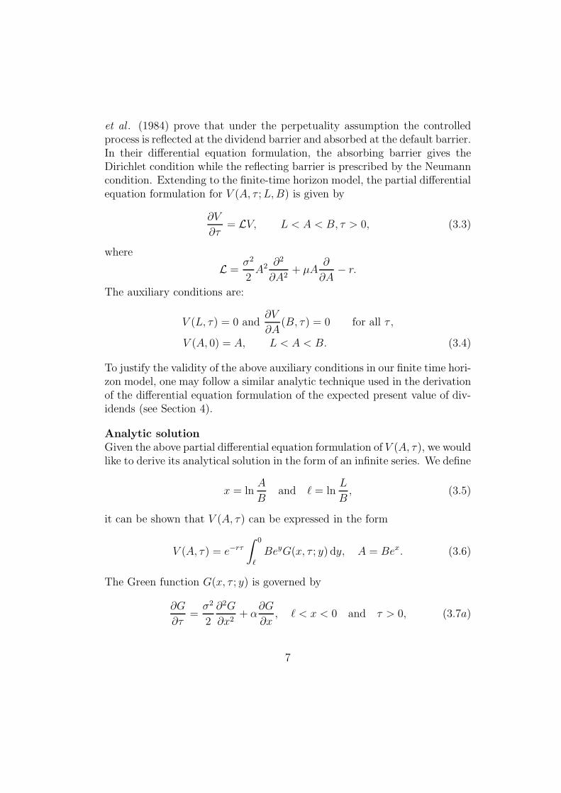
et al . (1984) prove that under the perpetuality assumption the controlledprocess is reflected at the dividend barrier and absorbed at the default barrier.In their differential equation formulation, the absorbing barrier gives theDirichlet condition while the reflecting barrier is prescribed by the Neumanncondition. Extending to the finite-time horizon model, the partial differentialequation formulation for V (A, τ ;L,B) is given by

∂V

∂τ= LV, L < A < B, τ > 0, (3.3)

where

L =σ2

2A2 ∂2

∂A2+ µA

∂

∂A− r.

The auxiliary conditions are:

V (L, τ) = 0 and∂V

∂A(B, τ) = 0 for all τ ,

V (A, 0) = A, L < A < B. (3.4)

To justify the validity of the above auxiliary conditions in our finite time hori-zon model, one may follow a similar analytic technique used in the derivationof the differential equation formulation of the expected present value of div-idends (see Section 4).

Analytic solutionGiven the above partial differential equation formulation of V (A, τ), we wouldlike to derive its analytical solution in the form of an infinite series. We define

x = lnA

Band ℓ = ln

L

B, (3.5)

it can be shown that V (A, τ) can be expressed in the form

V (A, τ) = e−rτ

∫ 0

ℓ

BeyG(x, τ ; y) dy, A = Bex. (3.6)

The Green function G(x, τ ; y) is governed by

∂G

∂τ=σ2

2

∂2G

∂x2+ α

∂G

∂x, ℓ < x < 0 and τ > 0, (3.7a)

7

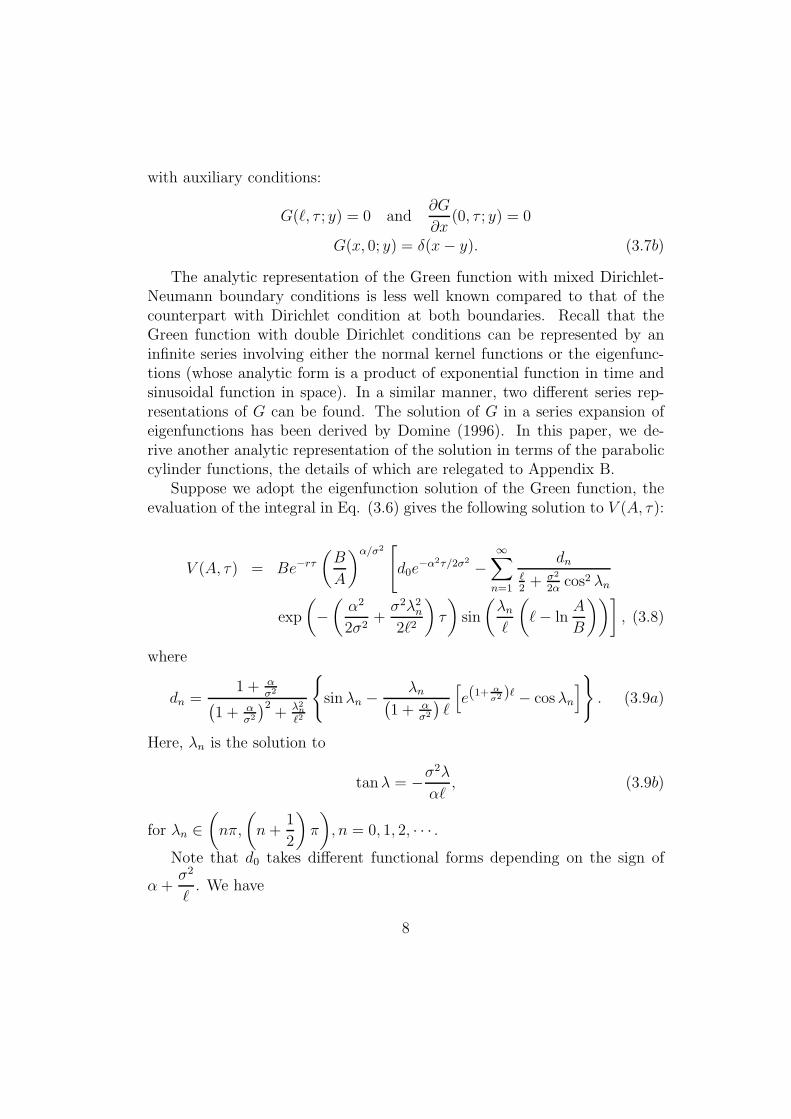
with auxiliary conditions:

G(ℓ, τ ; y) = 0 and∂G

∂x(0, τ ; y) = 0

G(x, 0; y) = δ(x− y). (3.7b)

The analytic representation of the Green function with mixed Dirichlet-Neumann boundary conditions is less well known compared to that of thecounterpart with Dirichlet condition at both boundaries. Recall that theGreen function with double Dirichlet conditions can be represented by aninfinite series involving either the normal kernel functions or the eigenfunc-tions (whose analytic form is a product of exponential function in time andsinusoidal function in space). In a similar manner, two different series rep-resentations of G can be found. The solution of G in a series expansion ofeigenfunctions has been derived by Domine (1996). In this paper, we de-rive another analytic representation of the solution in terms of the paraboliccylinder functions, the details of which are relegated to Appendix B.

Suppose we adopt the eigenfunction solution of the Green function, theevaluation of the integral in Eq. (3.6) gives the following solution to V (A, τ):

V (A, τ) = Be−rτ

(B

A

)α/σ2[d0e

−α2τ/2σ2 −∞∑

n=1

dn

ℓ2

+ σ2

2αcos2 λn

exp

(−(α2

2σ2+σ2λ2

n

2ℓ2

)τ

)sin

(λn

ℓ

(ℓ− ln

A

B

))], (3.8)

where

dn =1 + α

σ2(1 + α

σ2

)2+ λ2

n

ℓ2

sinλn − λn(

1 + ασ2

)ℓ

[e(1+ α

σ2 )ℓ − cosλn

]. (3.9a)

Here, λn is the solution to

tanλ = −σ2λ

αℓ, (3.9b)

for λn ∈(nπ,

(n+

1

2

)π

), n = 0, 1, 2, · · · .

Note that d0 takes different functional forms depending on the sign of

α +σ2

ℓ. We have

8

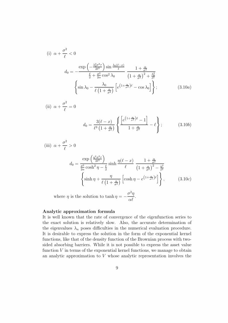
(i) α+σ2

ℓ< 0

d0 = −exp

(−λ2

0σ2τ

2ℓ2

)sin λ0(ℓ−x)

ℓ

ℓ2

+ σ2

2αcos2 λ0

1 + ασ2

(1 + α

σ2

)2+

λ20

ℓ2sinλ0 −

λ0

ℓ(1 + α

σ2

)[e(1+ α

σ2 )ℓ − cosλ0

]; (3.10a)

(ii) α+σ2

ℓ= 0

d0 =3(ℓ− x)

ℓ3(1 + α

σ2

)

[e(1+ α

σ2 )ℓ − 1]

1 + ασ2

− ℓ

; (3.10b)

(iii) α+σ2

ℓ> 0

d0 =exp

(η2σ2τ2ℓ2

)

σ2

2αcosh2 η − ℓ

2

sinhη(ℓ− x)

ℓ

1 + ασ2(

1 + ασ2

)2 − η2

ℓ2sinh η +

η

ℓ(1 + α

σ2

)[cosh η − e(1+ α

σ2 )ℓ]

, (3.10c)

where η is the solution to tanh η = −σ2η

αℓ.

Analytic approximation formulaIt is well known that the rate of convergence of the eigenfunction series tothe exact solution is relatively slow. Also, the accurate determination ofthe eigenvalues λn poses difficulties in the numerical evaluation procedure.It is desirable to express the solution in the form of the exponential kernelfunctions, like that of the density function of the Brownian process with two-sided absorbing barriers. While it is not possible to express the asset valuefunction V in terms of the exponential kernel functions, we manage to obtainan analytic approximation to V whose analytic representation involves the

9

exponential kernel functions only. Let τB = inft ≥ 0, At = B, and Edenote the expectation under the measure P, and recall [see Eq. 2.4a)]

AT = AT min

(1,

B

AT

0

)and At = At min

(1,B

At

0

),

the “initiation-state” asset value function for a term T can be expressed as

V (A, T ;L,B)

= e−rTE

[AT1n

bAT

0 >Lo]

= e−rTE

[AT1AT

0 >L1AT0 ≤B

]

+ e−rTE

[AT

B

AT

0

1B<AT0 1n

bAT

0 >Lo

]

= e−rTE

[AT1AT

0 >L1AT0 ≤B

]

+ e−rTE

[AT

B

AT

0

1B<AT0 1

min

„A

τB0 ,minτB≤t≤T At

B

At0

«>L

ff

]

= e−rTE

[AT1AT

0 >L

]

+ E

[AT

B

AT

0

1B<AT0 1

AτB0 >minτB≤t≤T At

B

At0

ff

(1

min0≤t≤T AtB

At0

>L

ff −1AT0 >L

)]. (3.11)

The second term in the last expression is small when the expectation of the

difference between the two indicator functions E

[1

min0≤t≤T AtB

At0

>L

ff −1AT0 >L

]

is small. This is true when A is sufficiently close to L.

We set Va(A, T ;L,B) to be e−rTE

[AT1AT

0 >L

], which is taken to be an

analytic approximation to V (A, T ;L,B). Since the original indicator func-tion 1n

bAT

0 >Lo in V has been replaced by 1AT

0 >L in Va, it becomes possible

to express Va in terms of the density function of the restricted Brownian

10

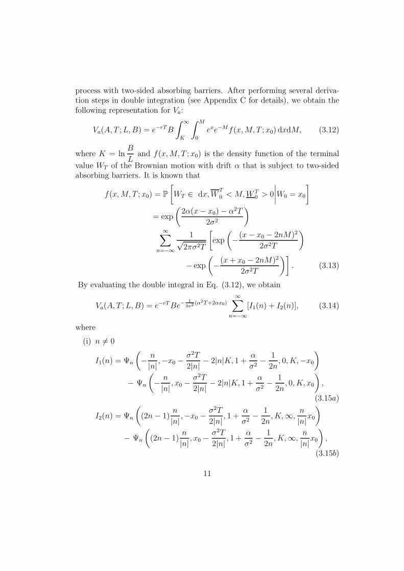
process with two-sided absorbing barriers. After performing several deriva-tion steps in double integration (see Appendix C for details), we obtain thefollowing representation for Va:

Va(A, T ;L,B) = e−rTB

∫ ∞

K

∫ M

0

exe−Mf(x,M, T ; x0) dxdM, (3.12)

where K = lnB

Land f(x,M, T ; x0) is the density function of the terminal

value WT of the Brownian motion with drift α that is subject to two-sidedabsorbing barriers. It is known that

f(x,M, T ; x0) = P

[WT ∈ dx,W

T

0 < M,W T0 > 0

∣∣∣∣W0 = x0

]

= exp

(2α(x− x0) − α2T

2σ2

)

∞∑

n=−∞

1√2πσ2T

[exp

(−(x− x0 − 2nM)2

2σ2T

)

− exp

(−(x+ x0 − 2nM)2

2σ2T

)]. (3.13)

By evaluating the double integral in Eq. (3.12), we obtain

Va(A, T ;L,B) = e−rTBe−1

2σ2 (α2T+2αx0)∞∑

n=−∞[I1(n) + I2(n)], (3.14)

where

(i) n 6= 0

I1(n) = Ψn

(− n

|n| ,−x0 −σ2T

2|n| − 2|n|K, 1 +α

σ2− 1

2n, 0, K,−x0

)

− Ψn

(− n

|n| , x0 −σ2T

2|n| − 2|n|K, 1 +α

σ2− 1

2n, 0, K, x0

),

(3.15a)

I2(n) = Ψn

((2n− 1)

n

|n| ,−x0 −σ2T

2|n| , 1 +α

σ2− 1

2n,K,∞,

n

|n|x0

)

− Ψn

((2n− 1)

n

|n| , x0 −σ2T

2|n| , 1 +α

σ2− 1

2n,K,∞,

n

|n|x0

),

(3.15b)

11

Ψn(a, b, c, d, f, g) =1

2n

eg2n

+ 12(

12n)

2σ2T

c

ecfN

(b− af

σ√T

)− ecdN

(b− ad

σ√T

)

+ ebca

+ 12(

ca)

2σ2T

[N

(af −

(b+ c

aσ2T

)

σ√T

)

− N

(ad−

(b+ c

aσ2T

)

σ√T

)]; (3.15c)

(ii) n = 0

I1(0) =L

B

[Φ(1, x0, 1 +

α

σ2, 0, K

)− Φ

(1,−x0, 1 +

α

σ2, 0, K

)],

(3.16a)

I2(0) = Φ(1, x0,

α

σ2, K,∞

)− Φ

(1,−x0,

α

σ2, K,∞

), (3.16b)

Φ(a, b, c, d, f) =1

ae

bca

+ 12(

ca)

2σ2T

[N

(af −

(b+ c

aσ2T

)

σ√T

)−N

(ad−

(b+ c

aσ2T

)

σ√T

)]. (3.16c)

Here, N(·) denotes the cumulative standard normal distribution function.We performed numerical calculations to testify the accuracy of the ana-

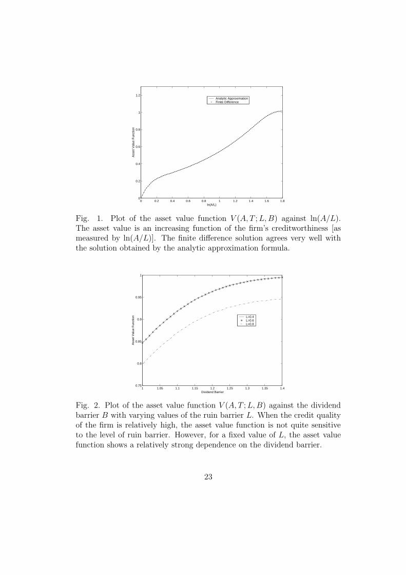
lytic approximation formula. In Figure 1, we show the plot of the asset valuefunction V (A, T ;L,B) against ln(A/L). The model parameter values usedin the calculations are: r = 0.08, σ = 0.15, T = 1, µ = 0.08, L = 0.2, B = 1.2.We compare the numerical approximation values of V obtained from the an-alytic approximation formula (3.14) with the numerical results obtained bysolving the partial differential equation for V [see Eqs. (3.5a,b)] using thefinite difference algorithm. As shown by the two curves in Figure 1, the fi-nite difference solution to the asset value function agrees very well with thesolution obtained from the analytic approximation formula even at relativelyhigh value of A/L. As revealed from Figure 1, V (A, T ;L,B) is an increasing

function of A, with a higher value of∂V

∂Awhen A is closer to the ruin barrier

L and a lower value of∂V

∂Awhen A is closer to the dividend barrier B.

We also examine the dependence of V (A, T ;L,B) on the dividend barrierB. Figure 2 shows the plot of V (A, T ;L,B) against B with varying values

12

of the ruin barrier L. Here, we take A = 1 and use the same set of modelparameter values as those in Figure 1 in the numerical calculations. Whenthe ratio L/A is small, corresponding to a high credit quality of the firm,the asset value function V is seen to be quite insensitive to the level of ruinbarrier. This is revealed by the overlapping of the asset value curves forL = 0.4 and L = 0.6 where A is taken to be 1. For a fixed value of L, theasset value function is an increasing function of dividend barrier since thedividend payout is less with a higher dividend barrier. The curves in Figure 2illustrate the phenomenon of the high sensitivity of V to the dividend barrierlevel.

4 Expected present value of dividends and

survival probability

In this section, we would like to derive the analytic formulation of the ex-pected present value of future dividends and the survival probability, andexamine their dependence on the creditworthiness of the firm, dividend bar-rier and ruin barrier.

Recall that At as defined in Eq. (2.4a) represents the non-ruined modifiedasset value at time t, which is the asset value process after dividends. LetdCt denote the non-negative amount of dividends paid in the time interval[t, t+ dt), and Ct is adapted to the filtration Ft. The stochastic differential

equation for At takes the form

dAt = µAt dt+ σAt dZt − dCt, (4.1)

with A0 = A. Let τ denote the first passage time of At to the ruin barrier L,that is,

τ = inft ≥ 0, At = L. (4.2)

Let F (A, T ;L,B) denote the expected present value of dividends at time zeroover a term T subject to ruin at a lower barrier L and dividend payout atan upper barrier B. We then have

F (A, T ) = E

[∫ T∧bτ

0

e−ru dCu

], (4.3)

13

where E denotes the expectation under the measure P. By considering afunction φ(A, τ) ∈ C2,1((L,B) × (0,∞)) that satisfies

∂φ

∂τ(A, τ) =

σ2

2A2 ∂

2φ

∂A2(A, τ) + µA

∂φ

∂A(A, τ) − rφ(A, τ) (4.4)

with auxiliary conditions:

φ(A, 0) = 0, L < A < B, (4.5a)

φ(L, τ) = 0 and∂φ

∂A(B, τ) = 1, τ > 0, (4.5b)

we would like to show that

F (A, T ) = φ(A, T ). (4.6)

To establish the result in Eq. (4.6), we follow the procedure outlined inFreidlin (1985). First, we apply the Ito calculus to obtain

e−r(τ∧bτ)φ(Aτ∧bτ , T − τ ∧ τ )

= φ(A, T ) +

∫ τ∧bτ

0

e−ru

[−∂φ∂τ

(Au, T − u) +σ2

2A2 ∂

2φ

∂A2(Au, T − u)

+ µA∂φ

∂A(Au, T − u) − rφ(Au, T − u)

]du

−∫ τ∧bτ

0

e−ru ∂φ

∂A(Au, T − u) dCu

+

∫ τ∧bτ

0

e−ru ∂φ

∂A(Au, T − u)Auσ dZu. (4.7)

Next, we set τ = T and take the expectation under P on both sides of theabove equation. By enforcing the partial differential equation for φ and the

boundary condition:∂φ

∂A= 1, we obtain

φ(A, T ) = E

[e−r(T∧bτ)φ(AT∧bτ , T − T ∧ τ )

]

+ E

[∫ T∧bτ

0

e−ru dCu

]. (4.8)

14

The last term is simply F (A, T ). It suffices to show that the first termvanishes. The first term can be split into two terms, namely,

E

[e−r(T∧bτ )φ(AT∧bτ , T − T ∧ τ)

]

= E

[e−rTφ(AT , 0)1bτ≥T

]+ E

[e−rbτφ(L, T − τ)1bτ<T

]. (4.9)

Both terms are seen to be zero by virtue of the auxiliary conditions: φ(A, 0) =0 and φ(L, τ) = 0, τ > 0. Hence, we obtain the result in Eq. (4.6).

Next, we would like to establish the relation between F (A, T ) and V (A, T ).If we let

ψ(A, τ) = φ(A, τ) −A + L, (4.10)

then the governing equation for ψ(A, τ) becomes

∂ψ

∂τ=σ2

2A2 ∂

2ψ

∂A2+ µA

∂ψ

∂A− rψ + (µ− r)A+ rL (4.11)

with auxiliary conditions:

ψ(A, 0) = L− A, L < A < B, (4.12a)

ψ(L, τ) = 0 and∂ψ

∂A(B, τ) = 0. (4.12b)

Now, the two boundary conditions (4.12a,b) are homogeneous, similar tothose of the asset value function V (A, τ) [see Eq. (3.5b)]. It can be shownthat the solution to ψ(A, τ) admits the following stochastic representation:

ψ(A, τ) = E

[e−rτ (L− AT )1τ<bτ

]

+ E

[∫ τ∧bτ

0

e−ru[(µ− r)Au + rL

]du

]. (4.13)

Setting τ = T and observing

V (A, T ) = E

[e−rT AT1T<bτ

], (4.14)

we can deduce the following relation between F (A, T ) and V (A, T ):

V (A, T ) = A− F (A, T ) − E

[Le−rbτ1T≥bτ

]

+ (µ− r)E

[∫ T∧bτ

0

e−ruAu du

]. (4.15)

15

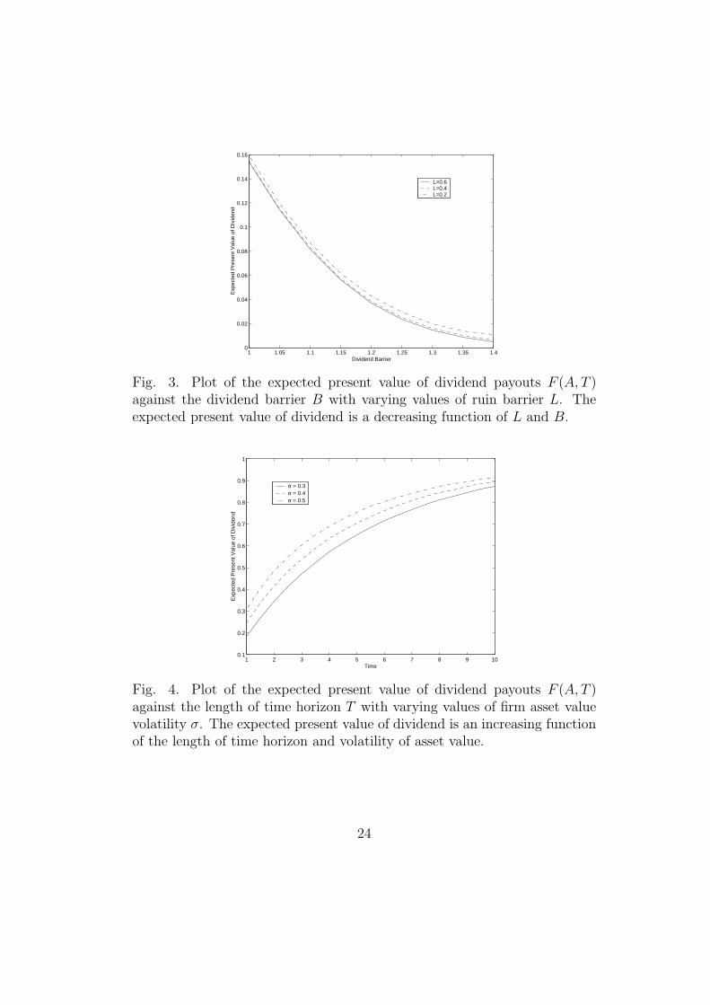
We performed numerical calculations to explore the dependence of theexpected present value of dividend payouts F (A, T ) on the ruin barrier L,dividend barrier B, volatility of the asset value process σ and length of timehorizon T . The plots in Figure 3 show that F (A, T ) is decreasing with respectto L and B. Also, F (A, T ) is seen to be highly sensitive to the change individend barrier. From Figure 4, we observe that F (A, T ) is increasing withrespect to σ and T . All these results agree with our intuition on the behaviorsof the expected present value of dividend payouts.

Another quantity of interest is the survival probability over a term T , asdefined by

S(A, T ) = P[τ > T ]. (4.16)

The partial differential equation formulation of S(A, T ) has been documentedin Paulsen (2003). It is quite straightforward to establish the following rela-tion between V (A, T ), F (A, T ) and S(A, T ):

V (A, T ) = A− F (A, T ) + Le−rTS(A, T ) − LE[e−r(T∧bτ)]

+ (µ− r)E

[∫ T∧bτ

0

e−ruAu du

]. (4.17)

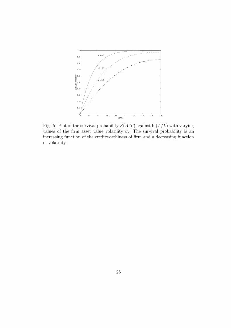
In Figure 5, we show the plot of the survival probability S(A, T ) againstln(A/L) with varying values of the firm asset value volatility σ. A highervalue of ln(A/L) indicates better creditworthiness of the firm, thus leadingto a higher survival probability. On the other hand, a higher asset valuevolatility leads to a higher chance of hitting the ruin barrier and consequentlya lower probability of survival.

5 Conclusion

In this paper, we derive the pricing formulation of the value function ofthe firm value process under the dividend barrier strategy and possibility ofruin. The upper dividend barrier is seen to be a reflecting barrier while thelower default barrier is an absorbing barrier. Our finite time dividend-ruinmodel resembles a path dependent option model with both the lookbackand barrier features. We have presented the analytic formulations of theexpected present value of the firm value, survival probability and expectedpresent value of dividends over a finite time horizon. Closed form analyticsolution to the value function of firm asset is obtained. In addition, a fairly

16

accurate analytic approximation formula is also derived. The mathematicalrelations between the asset value function, expected present value of dividendpayouts and survival probability of the finite time dividend-ruin model arepresented. Our numerical calculations show that the asset value function,survival probability and dividend payouts are quite sensitive to the dividendbarrier, firm’s creditworthiness and volatility of firm value.

AcknowledgementThis research was supported by the Research Grants Council of Hong Kong,HKUST6425/05H.

References

Asmussen, S., Taksar, M., 1997. Controlled diffusion models for optimaldividend pay-out. Insurance: Mathematics and Economics 20, 1-15.

Borodin, A.N., Salminen, P., 2002. Handbook of Brownian motion - Factsand Formulae, second edition, Birkhauser Verlag, Basel.

Choulli, T., Taksar, M., Zhou, X.Y., 2003. A diffusion model for optimaldividend distribution for a company with constraints on risk control.SIAM Journal of Control and Optimization 41, 1946-1979.

Chu, C.C., Kwok, Y.K., 2004. Reset and withdrawal rights in dynamic fundprotection. Insurance: Mathematics and Economics 34, 273-295.

Crosbe, P.J., Bohn, J.R., 1993. Modeling default risk. Report issued by theKMV Corporation.

Domine, M., 1996. First passage time distribution of a Wiener process withdrift concerning two elastic barriers. Journal of Applied Probability 33,164-175.

Domine, M., 1996. First passage time distribution of a Wiener process withdrift concerning two elastic barriers. Journal of Applied Probability 33,164-175.

Freidlin, M., 1985. Functional Integration and Partial Differential Equations.Princeton University Press, Princeton, New Jersey, USA.

Gerber, H.U., Shiu, E.S.W., 2003. Geometric Brownian models for assets andliabilities: From pension funding to optimal dividends. North AmericanActuarial Journal 7(3), 37-56.

17

Imai, J., Boyle, P., 2001. Dynamic fund protection. North American Actu-arial Journal 5(3), 31-51.

Longstaff, F.A., Schwartz, E.S., 1995. A simple approach to valuing riskyfixed and floating rate debts. Journal of Finance 50, 789-821.

Paulsen, J., Gjessing, H.K., 1997. Optimal choice of dividend barriers for arisk process with stochastic return on investments. Insurance: Mathe-matics and Economics 20, 215-223.

Paulsen, J., 2003. Optimal dividend payouts for diffusions with solvencyconstraints. Finance and Stochastics 7, 457-473.

Shreve, S.E., Lehoczky, J.P., Gaver, D.P, 1984. Optimal consumption forgeneral diffusions with absorbing and reflecting barriers. SIAM Journalof Control and Optimization 22, 55-75.

Taksar, M., 2000. Optimal risk and dividend distribution control models foran insurance company. Mathematical Methods of Operations Research51, 1-42.

18

Appendix A – Proof of Eq. (3.2)

Under the assumption of At

0 > B, we obtain

AT min

(1,

B

AT

0

)= AT

B

max(A

t

0, AT

t

)

= ATBmin

(1

At

0

,1

AT

t

)

= ATB

At

0

min

1,

B

AT

t

(B

At0

)

.

Furthermore, assuming At

0 > L, we have

1min0≤u≤T

»Au min

„1, B

Au0

«–>L

ff

= 1mint≤u≤T

»Au min

„1, B

Au0

«–>L

ff

= 18<:mint≤u≤T

24 AuB

At0

min

0@1, B

Aut

B

At0

1A

35>L

9=;

.

Combining the results, when At

0 > L and At

0 > B, we obtain

AT = ATB

At

0

min

1,

B

AT

t

(B

At0

)

18

<:mint≤u≤T

24 AuB

At0

min

0@1, B

Aut

B

At0

1A

35>L

9=;

,

and from which we can deduce the first relation in Eq. (3.2).

Appendix B – Green function with mixed Dirichlet-Neumann bound-ary conditionsLet U(x; y) denote the Laplace transform of G(x, τ ; y), where

U(x; y) =

∫ ∞

0

e−γτG(x, τ ; y) dτ.

19

The governing equation for U(x; y) is given by

σ2

2

d2U

dx2+ α

dU

dx− γU = 0, ℓ < x < 0,

with auxiliary conditions

U(ℓ) = U ′(0) = 0,

U ′(y+) − U ′(y−) = − 2

σ2and U(y+) = U(y−).

The solution to U(x, y) is found to be

(i) ℓ < x < y

U(x; y)

= D

"(β − α)e

−

β

σ2 (y−x+ℓ)+ (β + α)e

−

β

σ2 (ℓ−x−y)− (β − α)e

−

β

σ2 (x+y−ℓ)− (β + α)e

−

β

σ2 (x−y−ℓ)#

(ii) y < x < 0

U(x; y)

= D

"(β − α)e

−

β

σ2 (x−y+ℓ)+ (β + α)e

−

β

σ2 (ℓ−x−y)− (β − α)e

−

β

σ2 (x+y−ℓ)− (β + α)e

−

β

σ2 (y−x−ℓ)#

where D =e

α

σ2 (y−x)

2β[β cosh

(βℓσ2

)+ α sinh

(βℓσ2

)] and β =√α2 + 2γσ2. The fol-

lowing Laplace inversion formula [see p.642, Borodin and Salminen (2002)]is useful:

L−1γ

((2γ)bµ/2e−bx√2γ

sinh(t√

2γ) + z√

2γ cosh(t√

2γ)

)

=

∞∑

k=0

(−1)kk!

2kzk+1

k∑

ℓ=0

(−1)ℓ

(k − ℓ)!ℓ!cby(µ− k − 1, k + 1, t, x+ kt− 2ℓt), x > −t,

where γ is the dummy Laplace variable, z 6= 0, t > 0 and the function cey isdefined by

cey(µ, ν, t, z)

= 2eν∞∑

j=0

(−1)jΓ(ν + j)e−(eνet+ez+2jet)2/(4ey)

√2πy1+ eµ

2 Γ(ν)j!Deµ+1

(ν t+ z + 2jt√

y

),

ν ≥ 0, νt+ z > 0 and t > 0,

20

Deµ+1 is the parabolic cylinder function. One can then use the inversionformula to perform the Laplace inversion of U(x; y) to obtain G(x, τ ; y).

Appendix C – Derivation of analytic approximation formula (3.11)For the Brownian motion Wt with drift α and variance rate σ2, we write

W T0 = min

0≤t≤TWt and W

T

0 = max0≤t≤T

Wt, the density function f(x,M, T ; x0) of

the terminal valueWT conditional onW0 = x0 and subject to lower and upperabsorbing barriers at x = 0 and x = M , respectively, has been presented in

Eq. (3.13). The joint density of WT and WT

0 is given by

f(x,M, T ; x0) dxdM

= P

[WT ∈ dx,W

T

0 ∈ dM,W T0 > 0

∣∣∣∣W0 = x0

]

=∂f

∂M(x,M, T ; x0) dxdM.

We write A = A(0), K = lnB

Land let x0 = W0 = ln

A

Lso that x0 = 0 when

A = L. The restricted asset value process is given by

Va(A, T ;L,B) = E

[e−rTLeWT min

(1,

B

LeWT0

)1WT

0 >0

]

= e−rT

[L

∫ K

0

∫ M

0

exf(x,M, T ; x0) dxdM

+ B

∫ ∞

K

∫ M

0

exe−M f(x,M, T ; x0) dxdM

].

We let

I1 =

∫ K

0

∫ M

0

exf(x,M, T ; x0) dxdM

=

∫ K

0

∫ K

x

ex ∂f

∂MdMdx

=

∫ K

0

ex [f (x,K, T ; x0) − f(x, x, T ; x0)] dx

21

and

I2 =

∫ ∞

K

∫ M

0

exe−M ∂f

∂MdxdM

=

∫ K

0

∫ ∞

K

ex

[∂

∂M(e−Mf) + e−Mf

]dMdx

+

∫ ∞

K

∫ ∞

x

ex

[∂

∂M(e−Mf) + e−Mf

]dMdx

= −∫ K

0

ex L

Bf(x,K, T ; x0) dx−

∫ ∞

K

f(x, x, T ; x0) dx

+

∫ ∞

K

∫ M

0

exe−Mf(x,M, T ; x0) dxdM.

It is easily seen that f(x, x, T ; x0) = 0. Combining the above results together,we obtain

Va(A, T ;L,B) = e−rTB

∫ ∞

K

∫ M

0

exe−Mf(x,M, T ; x0) dxdM.

22

0 0.2 0.4 0.6 0.8 1 1.2 1.4 1.6 1.80

0.2

0.4

0.6

0.8

1

1.2

ln(A/L)

Ass

et V

alue

Fun

ctio

n

Analytic ApproximationFinite Difference

Fig. 1. Plot of the asset value function V (A, T ;L,B) against ln(A/L).The asset value is an increasing function of the firm’s creditworthiness [asmeasured by ln(A/L)]. The finite difference solution agrees very well withthe solution obtained by the analytic approximation formula.

1 1.05 1.1 1.15 1.2 1.25 1.3 1.35 1.40.75

0.8

0.85

0.9

0.95

1

Dividend Barrier

Ass

et V

alue

Fun

ctio

n L=0.4L=0.6L=0.8

Fig. 2. Plot of the asset value function V (A, T ;L,B) against the dividendbarrier B with varying values of the ruin barrier L. When the credit qualityof the firm is relatively high, the asset value function is not quite sensitiveto the level of ruin barrier. However, for a fixed value of L, the asset valuefunction shows a relatively strong dependence on the dividend barrier.

23

1 1.05 1.1 1.15 1.2 1.25 1.3 1.35 1.40

0.02

0.04

0.06

0.08

0.1

0.12

0.14

0.16

Dividend Barrier

Exp

ecte

d P

rese

nt V

alue

of D

ivid

end

L=0.6L=0.4L=0.2

Fig. 3. Plot of the expected present value of dividend payouts F (A, T )against the dividend barrier B with varying values of ruin barrier L. Theexpected present value of dividend is a decreasing function of L and B.

1 2 3 4 5 6 7 8 9 100.1

0.2

0.3

0.4

0.5

0.6

0.7

0.8

0.9

1

Time

Exp

ecte

d P

rese

nt V

alue

of D

ivid

end

σ = 0.3σ = 0.4σ = 0.5

Fig. 4. Plot of the expected present value of dividend payouts F (A, T )against the length of time horizon T with varying values of firm asset valuevolatility σ. The expected present value of dividend is an increasing functionof the length of time horizon and volatility of asset value.

24

0 0.2 0.4 0.6 0.8 1 1.2 1.4 1.6 1.80

0.1

0.2

0.3

0.4

0.5

0.6

0.7

0.8

0.9

1

ln(A/L)

Sur

viva

l Pro

babi

lity

σ = 0.3

σ = 0.4

σ = 0.5

Fig. 5. Plot of the survival probability S(A, T ) against ln(A/L) with varyingvalues of the firm asset value volatility σ. The survival probability is anincreasing function of the creditworthiness of firm and a decreasing functionof volatility.

25