finite state impedance-based control of a...
TRANSCRIPT

FINITE STATE IMPEDANCE-BASED CONTROL OF A POWERED
TRANSFEMORAL PROSTHESIS
By
AMIT BOHARA
Thesis
Submitted to the Faculty of the
Graduate School of Vanderbilt University in
partial fulfillment of the requirements
for the degree of
MASTER OF SCIENCE
in
Mechanical Engineering
December, 2006
Nashville, Tennessee
Approved:
Michael Goldfarb
Eric Barth
Nilanjan Sarkar

ii
Dedicated to my mother, Moti and
my brothers, Hari and Sandeep

iii
ACKNOWLEDGEMENTS
I would like to extend my sincere gratitude to Dr. Michael Goldfarb for providing the
opportunity to work on this very rewarding project. The many problems we faced provided
a great learning experience, and Dr. Goldfarb’s guidance was very helpful in guiding us
through many of the challenges. The considerable freedom he allowed us to experiment
and explore our own ideas, have helped me grow and develop a better perspective on
research and practical problem solving. So thank you once again. In addition, I would also
like to sincerely thank my committee members Dr. Eric J Barth and Dr. Nilanjan Sarkar for
graciously agreeing to volunteer their time to be in the committee.
Secondly, I would like to thank my partner in research, Frank Sup for his dedicated effort
and valuable insight. He did a great job of designing and assembling the leg that has made
this project possible. In addition, he displayed unparalleled bravery within the lab by
volunteering to put the leg on himself as a test subject for which I further extend my
appreciation. I have learned a lot from Frank and especially on his broad knowledge of the
field and his hard working ethics. Finally, no thanks to Frank would be complete without a
‘Thank you’ to Mrs. Sup for allowing him to stay past five during the busy times of the
project.
I would also like to thank our Post-Docs Kevin and Tom for their valuable suggestions
and insights during time of needs. I have been able to rely on Kevin for just about any
thing, from questions on technical matters, to political and cultural suggestions, and feel
fortunate to work in the room next to him. In addition, to all the wisdom that Tom brings
with him, I would first like to thank him for agreeing to put in the McMaster orders and
ensuring that things are always ordered and ‘faantastic’.

iv
Thanks are due to all my friends and peers in the graduate department and the Center for
Intelligent Mechatronics. I am especially thankful for their suggestions, help and good
natured humor. It has been a great experience and I wish them the best in the future.
Finally, I would like to thank my Mom and my Brothers for their support and patience.

v
TABLE OF CONTENTS
Page
DEDICATION ........................................................................................................ii
ACKNOWLEDGEMENTS..................................................................................... iii
LIST OF FIGURES..............................................................................................vii
LIST OF TABLES ................................................................................................. x
Chapter
I. MOTIVATION...................................................................................................1
II. PRIOR WORK .................................................................................................4
III. NORMAL WALK ..............................................................................................7
Four Gait Sub-Modes / States for a Normal Level Walk........................................ 9
IV. THE CONTROLLER ......................................................................................12
V. IMPEDANCE CHARACTERIZATION OF GAIT..............................................14
VI. MOMENT OF SUPPORT CHARACTERIZATION..........................................17
VII. IMPEDANCE CHARACTERIZATION OF BIOMECHANICAL GAIT ...............19
Stance Flexion / Extension .................................................................................. 20 Pre-Swing / Pushoff ............................................................................................. 28 Swing Flexion....................................................................................................... 33 Swing Extension................................................................................................... 35
VIII. CONTROLLER IMPLEMENTATION AND TESTING SETUP.........................37
IX. EVALUATION AND TUNING OF PROSTHESIS............................................40
Temporal Measure ............................................................................................... 41 Kinematic Measure .............................................................................................. 42 Tuning .................................................................................................................. 43

vi
X. EXPERIMENTAL RESULTS AND DISCUSSION...........................................45
XI. CONCLUSIONS.............................................................................................53
APPENDIX
A. Constrained Piecewise fitting of knee and ankle torques during normal speed level Walk ..............................................................................................................................55
B. Simulink Implementation of the Controller together with the Finite State Model ............................................................................................................................59
REFERENCES................................................................................................... 71

vii
LIST OF FIGURES
Figure Page
1-1. Joint power during one cycle for 75 kg normal subjects during fast walking................................................................................................ 2
3-1. Joint Angle conventions for human leg.......................................................... 7
3-2. Stick figure sketch of human walking over a single stride cycle .................... 8
3-3. Knee and Ankle angle pattern over a typical gait cycle ................................. 9
3-4. Stick figure sketch of Stance flexion / extension mode.................................. 9
3-5. Stick figure sketch of Push off / Pre-Swing mode........................................ 10
3-6. Stick figure sketch of swing flexion mode.................................................... 10
3-7. Stick figure sketch of swing extension mode............................................... 11
5-1. Piecewise fitting of knee and ankle torques during normal speed level walk ............................................................................................................ 15
7-1. Mass normalized Torque-Angle phase space relationship in the knee joint during Stance flexion / extension mode.............................................................. 20
7-2. Comparison between actual torques in the knee joint (Solid lines) with torque reconstructed from estimated parameters (Dashed lines) during stance flexion / extension mode .................................................................................................. 22
7-3. Mass normalized Torque-Angle phase space relationship in the ankle joint during early part of Stance flexion / extension mode.......................................... 23

viii
7-4. Mass normalized Torque-angle relationship in the ankle joint for stance flexion-extension (6-40%) phase ........................................................................ 24
7-5. Linear mass normalized torque-angle relationship in the ankle during middle of stance flexion-extension mode ........................................................................... 25
7-6. Characterization of movement of set point of the virtual spring at the ankle joint during for stance flexion-extension phase .......................................................... 26
7-7. Ratio of Knee and Ankle angle during push off ........................................... 28
7-8. Mass normalized torque-angle relationship in the knee joint during Push off mode .................................................................................................................. 29
7-9. Linear mass normalized torque-angle relationship in the Knee during
Push off .............................................................................................................. 30
7-10. Characterization of movement of set point of the virtual spring at the knee joint during Push off phase ................................................................................. 31
7-11. Mass normalized torque-angle relationship in the ankle joint during Push off mode .................................................................................................................. 32
7-12. Mass normalized torque-angle relationship in the knee joint during swing flexion mode ....................................................................................................... 34
7-13. Mass normalized torque-angle relationship in the knee joint during swing extension mode .................................................................................................. 36
8-1 . General Finite State model of gait .............................................................. 38
8-2 . Able-bodied testing adaptor for enabling development, testing, and evaluation of the prosthesis and controllers prior transfemoral amputee participation......... 39
10-1 . Average swing time of prosthetic and sound leg. Average heel strike period of gait trial ........................................................................................................... 47

ix
10-2 . Measured joint angles (degrees) for six consecutive gait cycles for a treadmill walk (1.8mph)..................................................................................................... 48
10-3 . Measured joint torques (N.m) for eight consecutive gait cycles for a treadmill walk (1.8mph)..................................................................................................... 50
10-4. Average Joint Power for eight consecutive gait cycles for a treadmill walk (1.8mph) ............................................................................................................ 50

x
LIST OF TABLES
Table Page
7-1. Impedance model parameters for stance flexion / extension phase of knee joint..................................................................................................................... 20
7-2. Impedance model parameters for early part of stance flexion / extension phase of ankle joint ....................................................................................................... 23
7-3. Stiffness parameters for linear part of stance flexion / extension phase of ankle joint..................................................................................................................... 25
7-4. Power fit parameters for the non-linear movement of set point of the virtual spring during stance flexion-extension ............................................................... 26
7-5. Stiffness parameters for linear part of Push off phase of knee joint ............ 30
7-6. Linear stiffness of the ankle joint during Push off mode .............................. 32
7-7. Linear damping parameters of the knee joint during Push off mode ........... 34
9-1. Kinematic variables useful for the evaluation of gait.................................... 43
10-1. Impedance parameters derived by experimental tuning............................ 52

1
CHAPTER I
MOTIVATION
Despite significant technological advances over the past decade, such as the introduction
of microcomputer-modulated variable damping, commercial transfemoral prostheses
remain limited to energetically passive devices. That is, the joints of the prostheses can
either store or dissipate energy, but cannot provide net positive power over a gait cycle.
The inability to deliver positive joint power significantly impairs the ability of these
prostheses to restore many locomotive functions including walking up stairs and up
slopes, running and jumping, all of which require significant net positive power at the knee
joint, ankle joint or both [1-8]. Further, even normal walking requires positive power output
at the knee joint and significantly net positive power at the ankle joint, (Fig 1-1) [1].
Transfemoral amputees walking with passive prostheses have been shown to expend up
to 60% more metabolic energy relative to healthy subjects during level walking [8] and
exert as much as three times the affected-side hip power and torque [1], presumably due
to the absence of powered joints. Prosthesis with the capacity to deliver power at the
knee and ankle joints would presumably address these deficiencies, and would
additionally enable the restoration of normal biomechanical locomotion.

2
Knee Joint Ankle Joint
Figure 1-1. Joint power during one cycle for 75 kg normal subjects during fast walking. Red represents positive power generated the joints during level walk [1, 3].
A significant bottleneck to the development of powered prosthetics has been the lack of
on-board power and actuation capabilities comparable to biological systems.
State-of-the-art power supply and actuation technology such as battery/DC motor
combinations suffer from low energy density of the power source (i.e., heavy batteries for
a given amount of energy), low actuator force/torque density, and low actuator power
density (i.e., heavy motor/gear head packages for a given amount of force or torque and
power output). However, recent advances in power supply and actuation for
self-powered robots, such as the liquid-fueled approaches described in [9-12] offer the
potential of significantly improved energetic characteristics relative to battery/DC motor
combinations and capable of biological scale energetic and power potential. This has
brought the potential of powered lower limb prosthesis to the near horizon and led to the
development of a prototype transfemoral prosthesis [41] that is intended to ultimately be
powered by the liquid-fueled approach. The developed prototype is a fully powered two
degree-of-freedom robot, capable of significant joint torque and power, which is rigidly
attached to a user. As such, the prosthesis necessitates a reliable control framework for
generating required joint torques while ensuring stable and coordinated interaction with
the user and the environment. This paper proposes an impedance based control
framework to produce normal gait patterns by characterizing joint behavior with a series of

3
finite states consisting of spring and damper behavior. The impedance based
characterization of knee and ankle joints allow for stable interaction while providing
intuitive means of tuning the model to facilitate desired gait pattern. This allows for greater
adaptability to different users in differing gait conditions.
4
CHAPTER II
PRIOR WORK
Prior work on transfemoral prosthesis can be understood in three broad categories, (a)
Passive mechanical devices, (b) Microcomputer-based modulated damping devices and
(c) Actively powered joints. Passive mechanical devices such as ‘peg’ legs or more
sophisticated ‘four-bar’ or ‘six-bar’ linkage mechanics provide a purely mechanical
framework for fulfilling simple necessitates of gait such as support and swing. However,
since they do not contribute much to the control aspect, they are omitted here in
discussion.
The initial ground work for the development of actively powered knee joints was the work
by Flowers et al., which took place during the 1970’s and 1980’s by Flowers [13], Donath
[14], Grimes et al. [16], Grimes [15], Stein [17], Stein and Flowers [18]. Specifically,
Flowers and Mann [19] developed a tethered electrohydraulic transfemoral prosthesis that
consisted of a hydraulically actuated knee joint tethered to a hydraulic power source and
off-board electronics and computation. They subsequently developed an “echo control”
scheme for gait control, as described by Grimes et al. [16], in which a modified knee
trajectory from the sound leg is played back on the contralateral side. In addition to this
prior work directed by Flowers, other groups have also investigated powered knee joints
for transfemoral prostheses. Specifically, Popovic and Schwirtlich [20] report the
development of a battery-powered active knee joint actuated by DC motors, together with
a finite state knee controller [21] that utilizes a robust position tracking control algorithm for
gait control [22]. They reported an increased cadence with lowering of metabolic energy

5
(O2 consumption) in clinical trials with amputees. However, the work was never
commercialized due to limitations in power capabilities. With regard to powered ankle
joints, Klute et al. [23-24] describe the design of an active ankle joint using pneumatic
McKibben actuators, although gait control algorithms were not described. Au et al. [25]
assessed the feasibility of an EMG based position control approach for a transtibial
prosthesis.
Since power limitations have hindered the development of active joints, a large number of
research has been devoted to the development of low power micro-computer controlled
damping joints. Since the knee joint exhibits damping behavior for a significant part of
level walk [1], this method does provide for feasible means of partial restoration of gait.
Bar et al. [26] reported on the development of a microcomputer controlled knee joint. The
gait was divided into 8 phases wherein damping at the knee joint was varied to enable
successful gait using information from sound side. Goldfarb [27] described the
development and control of knee prosthesis with modulated damping with no
dependencies on the sound side. Herr and Wilkenfeld [28] further describe a user
adaptive device with an autonomous algorithm that continuously adjusts the damping at
the knee joint to enable gait at differing speeds. Since all of these devices are passive
impedance-based, the control is limited to varying the damping values in different parts of
the gait stride. In addition, Kim and Oh [29] also report a MR based legs and related
tracking control.
Comparatively, since the ankle joint exhibits more of a spring like behavior during walk,
prosthetic ankle joints with spring return have become increasingly popular. The stiffness
is incorporated either using a mechanical spring or compliant material as in products
offered by companies such as Ossur. However, the ankle is a very active joint producing

6
impulsive power to aid the gait, and the spring behavior though helpful does not replicate
ankle joint behavior. With springs incorporated, issues of control are minimal since no
modulation of spring stiffness can be performed.
Finally, though no published literature exists, Ossur, a major prosthetics company based
in Iceland, has announced the development of both a powered knee and a self-adjusting
ankle. The latter, called the “Proprio Foot,” is not a true powered ankle, since it does not
contribute power to gait, but rather is used to quasistatically adjust the angle of the ankle
to better accommodate sitting and slopes. The powered knee, called the “Power Knee,”
utilizes an echo control approach similar to the one described by Grimes et al. [16]

7
CHAPTER III
NORMAL WALK
Walking is a highly coordinated behavior accomplished by intricate interaction of the
musculo-skeletal system, and hence a complete description is beyond the scope of this
work. Preliminary introduction to human walking can be obtained through Inman [33] and,
Rose [32]. Winter [34] provides a detailed analysis of kinematic, kinetic and muscle
activation patterns of human gait. Nonetheless, a short description of relevant features
and sub-modes of level walking is presented. While gait is essentially a 3-dimensional
activity, most of the work is done in the sagittal plane [1]. In addition, since the prosthesis
is constrained to operate in the sagittal plane, it also is the most relevant dimension. The
angle conventions used to describe gait are shown in Fig. 3-1.
Figure 3-1. Joint Angle conventions for human leg.
A stick figure diagram of a complete gait stride (cycle) is shown in Fig 3-2, with
accompanying joint angle behavior over a normal stride. The data is representative of

8
normal walking gait of a healthy population [1]. Joint functionality within each gait stride
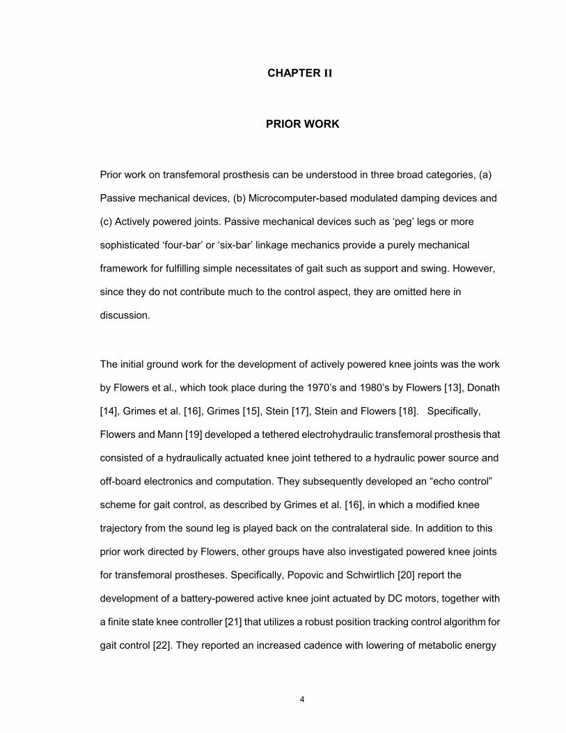
can be adequately captured by dividing the cycle into four distinct modes as sectioned in
Fig 3-3, each of which are described in further detail in subsequent paragraphs. Overall, a
typical gait can be divided into stance (load bearing) and swing (non-load bearing) phase,
each of which lasts approximately 60% and 40% of a gait cycle. A total of four functional
sub-modes (two for stance and two for swing) are identified and described in subsequent
sections.
Figure 3-2. Stick figure sketch of human walking over a single stride cycle. A normal gait stride cycle is described as the time interval between consecutive heel strikes of the same leg.
9
Figure 3-3. Knee and Ankle angle pattern over a typical gait cycle. Vertical lines represent the four distinct sub-modes within a gait period.
Four Gait Sub-Modes / States for a Normal Level Walk
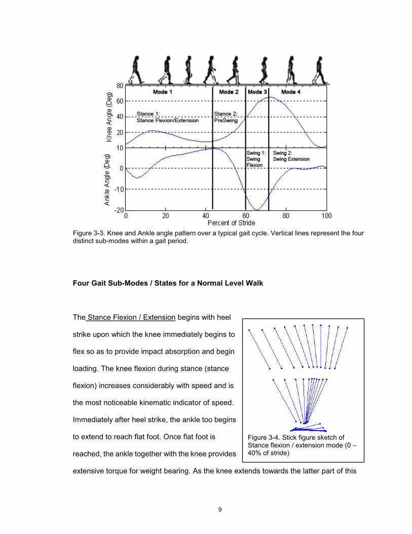
The Stance Flexion / Extension begins with heel
strike upon which the knee immediately begins to
flex so as to provide impact absorption and begin
loading. The knee flexion during stance (stance
flexion) increases considerably with speed and is
the most noticeable kinematic indicator of speed.
Immediately after heel strike, the ankle too begins
to extend to reach flat foot. Once flat foot is
reached, the ankle together with the knee provides
extensive torque for weight bearing. As the knee extends towards the latter part of this
Figure 3-4. Stick figure sketch of Stance flexion / extension mode (0 – 40% of stride)

10
mode, the ankle applies an increasing extensive torque in preparation for the push off
phase of gait.
The Pushoff / Pre-Swing is the active power
generation phase and begins as the ankle angle
becomes extensive (i.e. ankle velocity becomes
negative). The knee simultaneously begins to flex as
the ankle plantarflexes to provide push off power.
The push off combined with knee flexion also
prepares the leg for the swing phase and hence is
also referred to as “Pre-Swing”. The ankle and knee
joint together work in a relatively much more
coordinated manner during push off, so as to avoid any unnecessary jerks in the body,
during power generation in the ankle.
Early Swing (Swing Flexion) begins as the foot leaves
the ground and lasts until it reaches a maximum
flexion. The swing flexion is essential for proper
ground clearance and increases with speed.
However, the change in swing flexion with speed is
much less to that compared to stance flexion.
Individuals with gait disorders such as stiff-knee gait
often exhibit reduced swing flexion [35], making them
susceptible to stumbling and other problems. Healthy
maximum swing flexion angles usually lie between 60-70 degrees.
Figure 3-5. Stick figure sketch of Push off / Pre-Swing mode (40 – 60% of stride)
Figure 3-6. Stick figure sketch of swing flexion mode (60-73%) of stride

11
Late Swing (Swing Extension) mode represents the
forward swing of the leg, when the limb swings
forward in anticipation of heel strike. The muscles
are relatively dormant during early part of the swing,
with larger braking torques in the knee joint towards
the end to avoid impact during full extension. After
reaching full extension, the knee flexes slightly in
anticipation of heel strike.
The ankle torque remains relatively dormant during the swing phase, as it is not involved
in the forward swing of the leg and remains fairly neutral (close to zero degrees) in
anticipation of heel strike The knee joint in swing phase during slow and normal walking is
largely passive phase (Fig. 1-1) [1], since it only aids with stopping the knee, as the natural
dynamics of the body are usually sufficient in aiding the shank swing.
Figure 3-7. Stick figure sketch of swing extension mode (73-98%) of stride

12
CHAPTER IV
THE CONTROLLER
Unlike any prior work, this paper describes a method of control for a powered knee and
ankle joint together that enables natural, stable interaction between the user and the
powered prosthesis. The controller is similar to prior works described above in that it
divides gait into sub-modes or finite states and uses biomimetic characteristics to the
maximum extent possible. However, the overarching approach in all prior work (on the
control of active joints) has been to generate a desired joint position trajectory, which by its
nature utilizes the prosthesis as a position source. Such an approach poses several
problems for the control of powered transfemoral prosthesis. First, the desired position
trajectories are typically computed based on measurement of the sound side leg
trajectory, which 1) restricts the approach to only unilateral amputees, 2) presents the
problem of instrumenting the sound side leg, and 3) generally produces an even number
of steps, which can present a problem when the user desires an odd number of steps. A
subtler yet significant issue with position-based control is that suitable motion tracking
requires high output impedance, which forces the amputee to react to the limb rather than
interact with it. Specifically, in order for the prosthesis to dictate the joint trajectory, it must
assume a high output impedance (i.e., must be stiff), thus precluding any dynamic
interaction with the user and the environment.
Unlike prior works, the approach proposed herein utilizes an impedance-based approach
to generate joint torques. Such an approach enables the user to interact with the
prosthesis by leveraging its dynamics in a manner similar to normal gait [31], and also

13
generates stable and predictable behavior. The essence of the approach is to
characterize the knee and ankle behavior with a series of finite states consisting of
passive spring and damper behaviors, wherein energy is delivered to the user by
switching between appropriate spring stiffness (of the virtual springs) during state
transitions or by actively manipulating the equilibrium point (of the virtual springs). In this
manner, the prosthesis is guaranteed to be passive within each gait mode, and thus
generates power simply by switching between modes. Since the user initiates mode
switching, the result is a predictable controller that, barring input from the user, will always
default to passive behavior.
Though very apt and versatile, the human locomotion system is not a precise mechanism
like a robotic manipulator. The variability in joint torques from cycle to cycle during gait
indicates an adapting human locomotive system. In fact, Winter [31] reports that while the
sum of hip, knee and ankle joints over a gait stride have consistent repeatability, the
individual torques in the hip and knee joint have great variability. This demonstrates that
any external prosthesis needs to provide sufficient compliance for a more natural
interaction while delivering required torques. In addition, it is hypothesized that the central
nervous system often attempts to use the natural dynamics of the body to accomplish
physical tasks. By concretely defining the dynamic behavior of the prosthetic joints, a
better integration between the prosthetic user and the device can be expected. If optimal
joint dynamic behavior can be captured and consistently delivered to the user, it becomes
a natural extension of the body instead of an additional device such as wheel chair or
crutch that only has certain functional value. An impedance-based approach allows for
this dynamic characterization of knee and ankle joint, which in addition to providing the
required joint torques also provides a predictable behavior under different joint
configurations.

14
CHAPTER V
IMPEDANCE CHARACTERIZATION OF GAIT
Based loosely on the notion of impedance control proposed by Hogan [36] the torque
required at each joint during a single stride (i.e., a single period of gait) can be piecewise
represented by a series of passive impedance functions. A simple linear spring damper
model is proposed to characterize joint behavior within each gait mode, and a preliminary
regression analysis (see Appendix A) of gait data for normal walking (see Fig 5-1) from
Winter [1] indicates that joint torques can be approximated to a good degree as functions
of joint angle and velocity by the simple impedance model
θθθτ &be
k +−= )(1
(1)
The linear stiffness and damping are described by k1 and b, eθ is the equilibrium angle or
the set point, and the angle, θ and torque, τ , are defined as in Fig. 3-1. If the
coefficients b and k1 are constrained to be positive, then the joint will attempt to converge
to a stable equilibrium at eθθ = and 0=θ& within each gait mode. In addition, during
certain modes, where the joints act purely in a braking manner, non-linear elements can
be introduced to produce appropriate torque profile as long as the torque is constrained to
be opposite in sign of the joint velocity. Thus, in any given mode, the behavior is passive,
and will come to rest at a local equilibrium, thus providing a reliable and predictable
behavior for the human user.
The characterization of the control framework by relating torque to angle and velocity
states means the angular profile of the prosthesis need not be explicitly described in time.

15
This avoids the necessity of trajectory generation, which can be a cumbersome task to
define for all possible subsets of locomotion. In addition, specifying the position profile of
the prosthesis means the user needs to adapt to the prosthesis instead of the other way
around, which likely could increase rehabilitation time.
Effective impedance based characterization becomes possible due to segmentation of
gait into finite modes (see Fig 5-1) exhibiting distinct behaviors, as described in the earlier
sections. Such segmentation is made possible by analyzing torque phase space data
(torque-angle relationship), and identifying appropriate transitions between modes (see
Finite state Fig 8-1). Since the user initiates mode changes, the prosthesis barring input
from the user is constrained to a certain mode and thus to a certain dynamic behavior.
This is likely to facilitate better control and predictability of the device to the user.
0 10 20 30 40 50 60 70 80 90 100
-60
-40
-20
0
20
40
Impedance fit of Knee and Ank le Joint : Linear spring + Damper
Joint Torque
0 10 20 30 40 50 60 70 80 90 100-150
-100
-50
0
50
Percent of S tride
Knee
Ankle
S tance F lex ion /
E x tens ion
P re-Swing /
Push O ffSwing
Flex ionSwing E x tens ion
Ac tual
F it
Figure 5-1. Piecewise fitting of knee and ankle torques during normal speed level walk (averaged population data from Winter, 1991 scaled for a 75 kg adult) to a spring-damper impedance model. The vertical lines represent the segmentation of a gait stride into four distinct modes.

16
While a simple spring damper model provides an effective starting point to generating
necessary restoring torque, certain phases such as knee break during pre-swing, and the
stiffening of the ankle torque prior to push off, require more than the simple model
In such cases, the impedance model is augmented by altering the set-point angle of the
virtual spring in a dynamic manner. Such behaviors are described in a detailed analysis of
mode segmentation later in the thesis. In addition, though not shown in Fig 5-1, a
supplementary mode is added during early stance in the ankle joint to enable smooth
transition during heel strike.

17
CHAPTER VI
MOMENT OF SUPPORT CHARACTERIZATION
Transfemoral amputees often compensate the loss of knee and ankle joint by an extra
input in the hip joint [1]. In normal adults, the walking load is shared between various
joints. However, the sharing of joint loads during stance varies between individuals and
even between strides. As reported by Winter [31], while the algebraic sum of the hip, knee
and ankle joint (referred to as ‘Moment of Support’) is consistently positive and repeatable,
individual knee and hip joint even in normal adults show highly variable patterns during
stance period of normal walking (the ankle joint relatively is much more consistent). While
this observation is of qualitative nature, it does have significant relevance to the working of
transfemoral prosthesis. For instance, what specifically should the torque at the knee joint
be is a function of hip activity as well. Since, the user is likely to undergo sufficient
rehabilitation, it is assumed that this problem will be solved in reverse i.e. the user will
learn to recognize what hip moments are needed to interact in a useful manner with the
prosthesis as long as the prosthesis provides sufficient support. This lends further support
to the necessity of consistent behavior on part of the prosthesis. In addition, it appears that
as long as the knee torque is within a sufficient regime of values, gait is facilitated (though
ankle torque needs to be much more accurate). Hence, precise computation of torque
values may not be needed; rather simply approximation of joint dynamics is likely to
suffice and is the approach taken here. In the following chapters, we infer on a suitable set
of joint dynamic behavior based on biomechanical data [1] of a healthy population with the
intent to find general relationships that will allow for the generation of sufficient joint
torques to facilitate basic gait in a stable manner. Since, the idea is to establish a basic

18
framework; no attention is paid to optimizing gait variables such as energy efficiency,
workload in hip joints etc.

19
CHAPTER VII
IMPEDANCE CHARACTERIZATION OF BIOMECHANICAL GAIT
The knee and ankle have very different roles during the stance and swing phase of gait.
Since the ankle joint is directly in contact with the ground, it is the primary joint of
interaction with the external environment and hence dictates the overall energy input into
the body during walking. The ankle provides positive power while simultaneously also
guarding against collapse at the ankle joint. It is thus constrained to produce an extensive
torque through most of stance. The knee on the other hand, has a dual task of supporting
the body by providing sufficient torques at the joint, while also helping to ensure that
vertical trajectory of the body undergoes minimum diversion. During swing phase the knee
is primarily involved in limb advancement by swinging the shank through, as the ankle joint
remains relatively dormant. Though separate in their functionalities they do interact
significantly to facilitate forward movement in a smooth, stable manner.
In subsequent paragraphs, impedance behavior of the knee and ankle joint is
approximated from mass normalized population data [1]. Four functional modes or finite
states (Fig 5-1) of level walking are described in detail for both the knee and ankle joint.
As mentioned in the previous discussion, the goal here is to identify general relationships,
that “sufficiently reproduce” joint behavior. Attempt is made to validate the model against
three different speeds: slow, normal and fast, though the data for ‘normal’ is more
dominantly referred to.

20
Stance Flexion / Extension, 0% - 40%
Knee Joint
Figure 7-1. Mass normalized Torque-Angle phase space relationship in the knee joint during Stance flexion / extension mode (0 – 40%) of stride
During initial stance period the knee goes through a flexion-extension phase that serves to
absorb impact after heel strike, and to prevent unwanted vertical movement of the trunk.
As can be seen from the torque-angle phase space (Fig 7-1), there is dominant linear
relationship between the knee torque and angle. The characterization is further improved
by a damper that accounts for the hysteresis type loop behavior. The parameters for the
mode are determined by a least squares fit to be:
Table 7-1: Impedance model parameters for stance flexion / extension phase of knee joint shown in Fig 7-1
K1 b Set-Point
Fast 0.0635 0.0003 10.0000
Normal 0.0557 0.0003 12.0000
Slow 0.0604 0.0019 11.0000

21
The stiffness coefficients remain fairly constant through the three walking speeds and are
likely to explain the significant increase in stance flexion with speed. As the body moves
faster during walk the trunk has a greater momentum during heel strike thus causing the
knee joint to flex more. If the knee joint responded to higher speeds by a stiffer knee, then
it would oppose the natural dynamics that tended to cause knee flexion to a greater
degree.
Reconstructed torques from the estimated parameters indicate a relatively better fit for
slow and normal walking, though the general relationship is still visible in fast walking as
well. If deemed necessary during actual experiments, the fitting could be further improved
upon by adding an extra cubic term that maintains passive behavior while providing a
better fit, but simplicity was preferred given the necessity for experimental tuning. The
positive set point indicates that the knee joint initiates knee flexion by exerting a flexive
torque during early stance, and also helps the transition into push-off, by generating a
flexive torque towards the end of stance. Though, acting independently such flexive
torques would cause the knee to buckle; during gait, they help to counteract the extensive
torque exerted by the hip on the knee joint. This provides vertical support while avoiding
hyperextension in the knee.

22
Figure 7-2. Comparison between actual torques in the knee joint (Solid lines) with torque reconstructed from estimated parameters (Dashed lines) during stance flexion / extension mode (0
– 40%) of stride
Ankle Joint
The ankle joint exhibits two different functionalities during the stance flexion/extension
period. Immediately following heel strike, the angle applies a dorsiflexive torque, to ease
the foot into the ground and avoid any slapping (as see in drop foot gait). This behavior
last for a very short period (0% - 6%), until the foot touches the ground and ankle angle
begins to flex. The ankle stiffness is relatively less compared to later in the stance to allow
for more compliant interaction with the ground.

23
-6 -4 -2 0 20
0.02
0.04
0.06
0.08
0.1
0.12
0.14
1%
4%
Ank le Angle (deg)
Ankle Torque
A nk le Joint charac terization for 0-4%
S low
Normal
Fas t
Figure 7-3. Mass normalized Torque-Angle phase space relationship in the ankle joint during early part of Stance flexion / extension mode (0 – 4%) of stride
Table 7-2: Impedance model parameters for early part of stance flexion / extension phase of ankle joint shown in Fig 7-3
K1 b
Set-Point (deg)
Fast 0.0325 0.0002 1
Normal 0.0125 0.0003 1
Slow 0.0105 0.0001 -1
Once the foot reaches the ground, the loading of the ankle begins. The torque-angle
space behavior (Fig 7-4) initially exhibits a linear relationship between torque and angle,
and this plantarflexive torque is likely aimed at preventing buckling at the ankle joint.
Once, the ankle joint is flexed past a certain threshold, the ankle produces an increasingly
larger force that increases non-linearly until the joint produces sufficient torque to begin
extension. This onset of non-linear behavior could in some sense be regard as the
beginning of push off, since the amount of torque the persons responds with at this phase
plays a significant role in determining the speed of the person. One notable feature of the
ankle torque during this phase is that for most of period, the torque is higher for slower
speeds, which could be considered counter-intuitive during first glance. However, less
flexive resistance in the ankle joint allows the shank to rotate ahead fast and more easily.

24
Later during the unloading or propulsive push off we will observe higher flexive torques
with faster speeds.
-8 -6 -4 -2 0 2 4 6 8 10-1.4
-1.2
-1
-0.8
-0.6
-0.4
-0.2
0
0.2
6% 6%
40%
6%
Ankle Angle (deg)
Ankle Torque
Ankle Joint characterization for 6-40%
Slow
Normal
Fast
Figure 7-4. Mass normalized Torque-angle relationship in the ankle joint for stance
flexion-extension (6-40%) phase
The overall ankle behavior is captured by initially determining the stiffness of the ankle
during the linear phase (see Fig 7-5). Once the threshold is crossed, the non-linear
increase in the force is characterized as a non-linear movement of the set point, while the
stiffness remains constant. The stiffness (Table 7-3) in the ankle appears slightly larger
with speed, though the set point of the ankle spring ensures that smaller torques are
produced so as to minimally impede joint motion without allowing buckling.

25
-8 -6 -4 -2 0 2 4 6 8-0.7
-0.6
-0.5
-0.4
-0.3
-0.2
-0.1
0
0.1
0.2
6% 6%
22%
6%
Ankle Angle (deg)
Ankle Torque
Ankle Joint characterization for 6-22%
Slow
Normal
Fast
Figure 7-5. Linear mass normalized torque-angle relationship in the ankle during middle of stance flexion-extension mode (6-22% of stride). Solid lines indicate actual data, while the fit is represented by dashed lines.
Table 7-3 Stiffness parameters for linear part of stance flexion / extension phase of ankle joint shown in Fig 7-5
K1
Set-Point (deg)
Fast 0.0621 -2
Normal 0.0590 -5
Slow 0.0569 -6
The movement of the ankle set point (Fig 7-6.) shows contrasting behavior at different
speeds. At slow speeds the change in set point is initiated at less ankle flexion, and
increases at a slower rate. In contrast, the set point change during fast walking happens
with no change in ankle angle. This sudden movement of the set point could be explained
through sudden release of the contracting muscle to generate a propulsive torque. The
overall principle of torque generation in the ankle during this mode is characterized by the
following principle using a power fit to describe the movement of the set point:
)(1 ek θθτ −= , Where, 0θθ =
e for
thresholdθθ ≤

26
0)( θθθθλ+−⋅=
thresholdA
e for
thresholdθθ >
Where, 0θ And 1k are the set point and stiffness value characterized in Table 7-3. A fit for
the movement of the set point is shown in Fig 7-5. The fit parameters are stated in Table
7-4.
-6 -4 -2 0 2 4 6 8 10-16
-14
-12
-10
-8
-6
-4
-2
0
Ankle Angle (deg)
Ankle S
et Point (deg)
Set-Point characterization for 8-40%
Slow
Normal
Fast
Figure 7-6. Characterization of movement of set point of the virtual spring at the ankle joint during for stance flexion-extension (6-40%) phase. Solid lines indicate actual data, while dashed lines represent the fit.
Table 7-4. Power fit parameters for the non-linear movement of set point of the virtual spring during stance flexion-extension (6-40%) phase as shown in Fig 7-6.
A λ Threshold
Fast -0.1145 7.729
-6
Normal -0.1145 2.517 -4
Slow -0.1145
2.089
0
The choice of a power fit to represent the movement of the set point has a few attractive
features. The speed can be characterized by varying ‘λ ’ and threshold, both of which are

27
very intuitive, since one almost needs to be adjusted in inverse of the other. The
coefficient ‘A’ yields a good fit at a given constant value and need not be adjusted if the
tuning is limited to the aforementioned two variables. In addition, distinctly different curves
representing very different behaviors can be generated only by slight adaptation of the
tuning variables.
The power fit characterization of the set point does not lend itself to the normal passivity
characterization of the spring damper model. However, the passive behavior of the ankle
is still guaranteed since the set point movement is limited to the mode where the ankle
torque is negative while the angle is flexing (positive velocity), thus constraining the ankle
power to be negative. As soon as the movement of the set point causes the ankle velocity
to become positive (extensive) and the ankle power becomes positive, the ankle joint
switches onto the next mode, where the spring-damper joint characterization is resumed.
Thus, the introduction of the power curve only allows for a better characterization of
non-linear ankle torque characterization without risk of instability.

28
Pre-Swing / Pushoff, 42% - 60%
Knee Joint
Once the ankle becomes extensive the knee simultaneously begins to flex to avoid
unnecessary excursions in the trunk while the ankle generates forward propulsive power
through active extension in the joint. The coordination between the ankle and knee joint is
relatively higher during this mode. In fact, the knee and ankle angle vary linearly with
respect to each other during this mode, irrespective of the walking speed (See Fig 7-7).
The ratio of the joint angles is approximately 1.4 during this phase, and remains relatively
unchanged during different tasks. This is indicative of the high degree of positional
coordination necessary for the proper execution of the push off phase.
-15 -10 -5 0 5 105
10
15
20
25
30
35
40
Ankle Angle (deg)
Knee Angle (deg)
Knee Vs Ankle Angle during Push Off (42-58%)
Fast
Slow
Normal
Figure 7-7. Ratio of Knee and Ankle angle during push off
The knee torque-angle behavior for this mode is shown in Fig 7-8. The knee joint is in
maximum extension towards the end of the stance flexion-extension mode, and begins
knee break by initiating flexion through a flexive torque. Once, the knee flexes beyond the

29
set point and the knee torque becomes extensive (negative), the joint behaves as a
non-linearly softening spring (the ankle in contrast behaved as a hardening spring during
the earlier stance phase).
5 10 15 20 25 30 35 40 45 50-0.4
-0.3
-0.2
-0.1
0
0.1
0.2
0.3
40%
Knee Angle
Knee Torque
K nee Joint charac teriz ation for 40-60%
S low
Normal
Fas t
Figure 7-8. Mass normalized torque-angle relationship in the knee joint during Push off mode
(40-60% of stride).
The characterization of knee torque during phase space is done by modeling a spring with
a set point dependent on the knee angle. The knee stiffness is specified during the initial
flexive torque behavior and is held constant through the entire time. The stiffness is for all
practical purposes uniform over various walking speeds, and it is only a differing set-point
that distinguishes the torque behavior during various walking speeds

30
6 8 10 12 14 16 18 20-0.4
-0.3
-0.2
-0.1
0
0.1
0.2
0.3
42%
Knee Angle
Knee Torque
K nee Joint charac terizat ion for 42-52%
S low
Normal
Fas t
Figure 7-9. Linear mass normalized torque-angle relationship in the Knee during Push off (42-52% of stride).
Table 7-5. Stiffness parameters for linear part of Push off phase of knee joint shown in Fig 7-9
K1
Set-Point (deg)
Fast 0.037 10
Normal 0.0311 17
Slow 0.0300 17
The movement of the knee set point under the assumption that the stiffness is constant for
various speeds is shown in Fig 7-10. The movement of the set point is modeled as a
quadratic function of the knee angle after the knee torque becomes extensive. It is
important to note that passivity of the controller would not be maintained under a quadratic
relationship if the knee torque were positive since the joint would produce positive power
(note that the knee velocity is positive). However, since the set point is moved in a
quadratic relationship after the knee torque becomes extensive (i.e. negative), the joint is
limited to negative power at the joint, and thus constrained to be passive. The final knee
joint behavior for this mode can be characterized as:
)(1 ek θθτ −= , Where, 0θθ =
e for 0θθ ≤
002
0 )0.424()( 0.0153 θθθθθθ +−+−=e
for 0θθ >
31
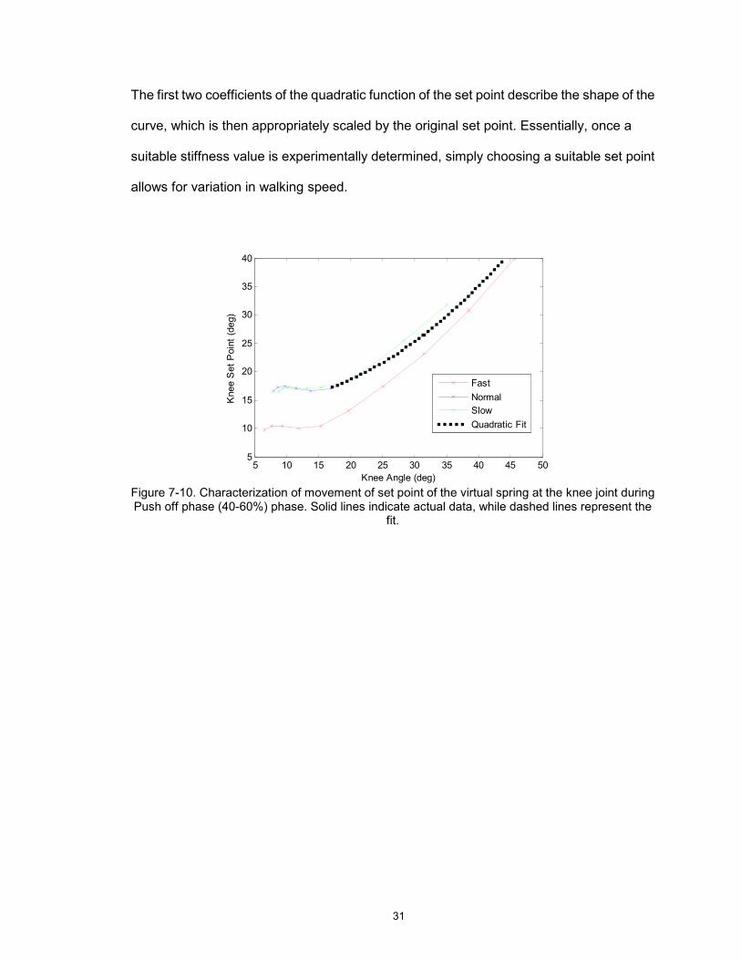
The first two coefficients of the quadratic function of the set point describe the shape of the
curve, which is then appropriately scaled by the original set point. Essentially, once a
suitable stiffness value is experimentally determined, simply choosing a suitable set point
allows for variation in walking speed.
5 10 15 20 25 30 35 40 45 505
10
15
20
25
30
35
40
Knee Angle (deg)
Knee S
et Point (deg)
Fast
Normal
Slow
Quadratic Fit
Figure 7-10. Characterization of movement of set point of the virtual spring at the knee joint during Push off phase (40-60%) phase. Solid lines indicate actual data, while dashed lines represent the
fit.

32
Ankle Joint
The push off phase in the ankle joint begins when the ankle becomes extensive. This is
the unloading phase in the ankle joint, as the ankle provides positive power to aid push off.
The torque space behavior of the ankle joint during this phase is fairly linear and hence
lends itself well to characterization as a linear spring (see Fig 7-11). The parameters
(Table 7-6) indicate that the set point rather than the stiffness needs to be adjusted to
enable different speeds.
-20 -15 -10 -5 0 5 10-2
-1.5
-1
-0.5
0
0.5
42%
60%
Ankle Angle (deg)
Ankle Torque
Ankle Joint characterization for 42-60%
Slow
Normal
Fast
Figure 7-11. Mass normalized torque-angle relationship in the ankle joint during Push off mode (42-60% of stride). Solid lines indicate actual data, while dashed lines represent the fit.
Table 7-6. Linear stiffness of the ankle joint during Push off mode shown in Fig.7-11
K1
Set-Point (deg)
Fast .083 -17
Normal .073 -13.5
Slow .074 -10

33
The discussion of joint behavior during swing phase is limited to the knee joint since it has
a more dominant role during this phase. The ankle torque during swing is small and is
simply characterized as a weak spring with a set point close to zero degrees. The knee
on the other hand swings back to reach a maximum swing flexion angle before swinging
forward to near full extension in anticipation of heel strike. Previous controller for variables
impedance knees [9, 28] have characterized swing phase as an entirely passive mode.
Human gait data does indicate the swing phase as primarily passive, where the natural
dynamics are sufficient to induce swinging, and the joint primarily works as a brake.
The inertial properties of the human leg and the prosthesis are different, and this becomes
very apparent during swing. During stance the overall forces imposed on the prosthesis
are much higher, and the prosthesis is in a higher output impedance mode, thus
precluding any influence of the physical dynamics of the prosthesis. However, during
swing, a human leg is able to swing fairly well and the impedance at the joint is small.
Comparatively, the back drivability of pneumatic actuators impedes free swinging motion
of the prosthesis, though the issue is partly corrected by adding feed forward velocity
compensation, human like low impedance is still difficult to achieve. Hence, the analysis of
knee behavior during swing using biomechanical data may not be directly applicable to a
prosthesis. Nonetheless, a simple spring damper model is still found to be fairly close to
actual biomechanical data and discussed in subsequent as a feasible model.
Swing Flexion (60 – 72 %)
Swing flexion begins immediately after toe off, as the shank swings back while the hip is
swinging forward. A steady extensive braking torque causes the knee joint to achieve
some amount of maximum flexion before the forward swing. This flexion angle often

34
referred to as “maximum swing flexion” angle is critical to achieving ground clearance,
since it allows the hip to travel sufficiently forward before the shank swings through. A
healthy swing flexion for normal adults is usually between 60-70 deg and increases with
walking speed [1]. The simplest characterization of knee joint in this mode is a simple
damper. This has the advantage of presenting only a single tuning variable (the damping
coefficient) and a single measure of the outcome (maximum swing flexion angle), with a
clear defined relationship between the two.
-100 0 100 200 300 400-0.2
-0.15
-0.1
-0.05
0
62%
Knee Vel
Knee Torque
K nee Joint charac terization for 62-72%
S low
Normal
Fas t
Figure 7-12. Mass normalized torque-angle relationship in the knee joint during swing flexion mode (62-72% of stride). Solid lines indicate actual data, while dashed lines represent the fit.
Table 7-7. Linear damping parameters of the knee joint during Push off mode shown in Fig. 7-12
Damping Coefficient
Fast 644e-6
Normal 238e-6
Slow 174e-6
The biomechanical data does display a linear damping (Fig 7-12), and the damping values
are higher for fast walking speeds (Table 7-7). This increase in damping protects the knee
joint from flexing to larger than desired angle as the joint velocity increases with increase
in walking speed. If desired flexion is not achieved even when the damping is set to zero,
35
then an additional spring element can be added with a set point less than the desired
swing flexion so that it provides some amount of positive power to swing the leg up to the
desired angle. However, in most prosthesis with variable impedance mechanisms,
velocity dependent damping are the norm and have appeared to function well [9, 28],
though they can be powerless if under minimum friction the desired swing flexion is not
achieved [28]
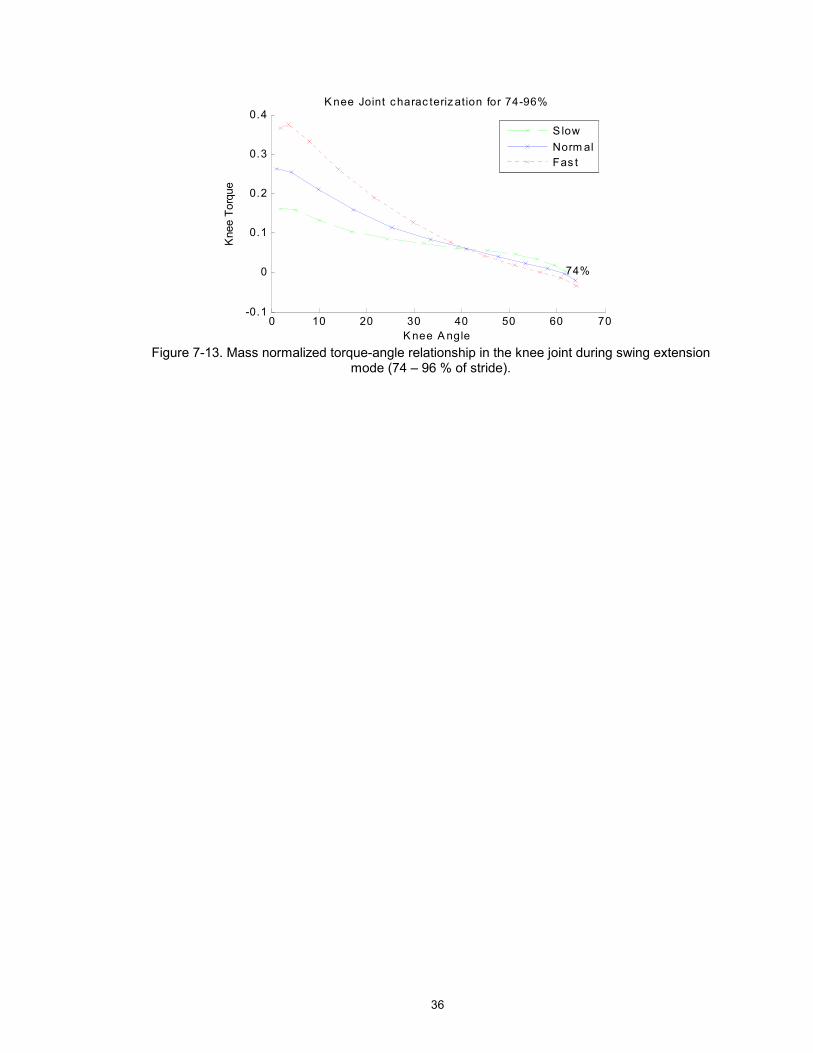
Swing Extension (72-98%)
Once the maximum swing flexion is achieved, the leg swings forward until it reaches close
to full extension. The braking in the knee joint during forward swing is fairly non linear (Fig
7-13). The torque remains low initially allowing for a free swing and increases rapidly as
the leg approaches full extension. Due to the stiff back drivability of pneumatic actuators
and limited bandwidth, a free swing of the prosthesis is hard to attain (even with feed
forward velocity compensation) and hence the normal biomechanical profile (Fig 7-13.)
may be not be applicable. However, the goal in the forward swing is fairly well defined, as
the leg has to swing from a given initial angle to close to full extension in some given time
period in a smooth manner. As an alternative solution, a simple spring and damper model
is used, and pure damping behavior during swing is replaced by an initial injection of
power in the beginning of the swing that is later braked by the spring and damper together
to avoid impact at full extension. The stiffness of the joint is tuned to adjust the time the leg
takes to swing through (as stiffness is directly related to frequency in a
mass-spring-damper system) and the position of the spring set point is adjusted to stop
the knee angle at the desired value. Hence, the pure passive functionality of the knee joint
in normal gait, is replaced by a simple spring damper that provides easy tunability.
36
0 10 20 30 40 50 60 70-0.1
0
0.1
0.2
0.3
0.4
74%
Knee Angle
Knee Torque
K nee Joint charac teriz ation for 74-96%
S low
Normal
Fas t
Figure 7-13. Mass normalized torque-angle relationship in the knee joint during swing extension
mode (74 – 96 % of stride).

37
CHAPTER VIII
CONTROLLER IMPLEMENTATION AND TESTING SETUP
The finite state impedance-based controller was implemented using Matlab (7.3) and
Simulink (6.5). The gait algorithm was implemented as a Finite state machine in Simulink
using State flow model (Fig 8-1). The various gait modes described are each treated as an
individual state and appropriate transitions between the two are defined. The overall
Simulink implementation is available in Appendix B. As this is meant to be a preliminary
implementation of level walking at a pre-defined speed, extra transitions between gaits are
not included to avoid unnecessary chattering as can happen with a switching control
algorithm. A proportional control method was implemented to provide low level force
control in the actuator and gains were experimentally tuned to allow best force tracking in
a stable manner. A National Instrument Data Acquisition card (PCI-6031E) was used to
electrically interface to the tethered prosthesis.

38
Figure 8-1. General Finite State model of gait. Each box represents a possible state and the appropriate transition between states are specified
The gait control strategy was implemented on the tethered prosthesis prototype on a
healthy subject using an able-bodied testing adaptor as shown in Fig. 8-2. The adaptor
consists of a commercial adjustable locking knee immobilizer (KneeRANGER-Universal
Hinged Knee Brace) with an adaptor bracket that transfers load from the subject to the
prosthesis. Since the prosthesis remains lateral to the immobilized leg of the healthy
subject, the adaptor simulates transfemoral amputee gait without geometric interference
from the immobilized leg. While the adapter allows for preliminary testing of the gait
control algorithm, the setup does involve certain drawbacks in simulating prosthetic gait,
some of which include 1) compliance of the soft tissue interface between the device and
user (more so than exhibited by a limb/socket interface), 2) “parasitic” inertia of the intact
lower limb (i.e., in addition to the inertia of the prosthesis), and 3) asymmetry in the frontal
and axial planes which results in a larger than normal planar moments (i.e., as seen in
Fig 8-2). Despite these, the adaptor provides a reasonable facsimile of amputee gait, and
enables testing of the device and proposed impedance-based control approach.

39
Figure 8-2. Able-bodied testing adaptor for enabling development, testing, and evaluation of the prosthesis and controllers prior transfemoral amputee participation.
Gait trials were performed on a treadmill, which provided a controlled walking speed and
enabled enhanced safety monitoring, including a safety suspension harness and the use
of handrails. The prosthesis was provided a 2Mpa (300 psig) pressure supply through a
tether. Biomechanical impedance parameters estimated from population data [1] were
used as the starting point and iteratively tuned through feedback from the user, recorded
gait profiles and video to produce a gait pattern that seemed satisfactory to the user and
showed reasonably good gait profile.

40
CHAPTER IX
EVALUATION AND TUNING OF PROSTHESIS
The quality of gait can be assessed in both qualitative and quantitative terms. Foremost,
the comfort and feedback of the user needs to be taken into consideration and is also the
most useful in evaluating the contribution of a prosthetic device. The user is often
perceptive to power input from the device (e.g. ankle push off torque) and its overall
dynamics. In addition, a simple visual assessment of gait can reveal obvious gait
pathology such as excessive and asymmetrical movements in the body. While qualitative
analysis provides a very reasonable and appropriate method of evaluating gait, it does
have certain limitations. For instance, gait trials lasting a prolonged period allow the user
to adjust to different prosthetic behavior, and this can affect the user feedback. A user may
easily get accustomed to working with less than desired push off at the ankle joint or
non-ideal behavior during heel strike, and thus may not provide adverse feedback once he
has adapted to these disturbances in the device. In addition, visual assessment, even by
experts, cannot be relied on consistently and even when a problem is visually observed
the cause is difficult to determine [37]. Hence, it is necessary to have some amount of
quantitative variables that can be consistently measured to assess the quality of gait
without reliance on human intuition.
While a single quantitative measure of the quality of gait is hard to define, certain pointers
do exist as guides. Quantitative analysis of gait can be done by analyzing
temporal-spatial, kinematic, kinetic and energy related parameters [38]. The overall data
41
that can be collected for evaluation purposes are limited by the set of sensors available in
the laboratory setting. The sensor set used are as follows:
(a) Knee and Ankle Potentiometer
(b) Load sensors to measure joint torques
(c) Socket load cell above prosthetic knee together with footswitches to detect heel
strike and toe off events on prosthetic and sound side.
A clinical assessment of gait of an amputee is likely to involve a more comprehensive
measurement of gait parameters. However, since this experiment constitutes a
preliminary study of assessment and tuning of prosthesis, only a minimal set of
parameters are chosen so as to keep the entire process compact and manageable. The
goal of the entire tuning and gait evaluation process is to (a) improve temporal symmetry;
(b) reproduce healthy looking kinematic data and (c) Minimize jerks and significant
physical asymmetry in walking. Each of these domains is discussed in further detail in the
following sections.
TEMPORAL MEASURE
While amputees markedly walk at slower self-selected speeds, the treadmill constrains
the user to a pre-selected speed. However, the stance and swing times on normal and
prosthetic leg spent to achieve the desired speed may not be symmetrical. In fact,
amputees using passive knee joints often demonstrate a slower than normal swing phase
[39]. A significant asymmetry in either stance time or swing time (they are correlated by
cadence) is often indicative of non-optimal gait. In our particular control strategy, the user
has direct control over the leg during stance and relatively less control over the prosthesis
during swing. . If the prosthesis is taking slower or longer than a nominal duration during

42
swing, than it also forces asymmetry during the stance times. Hence, the first goal is to
ensure that swing times for both prosthetic and sound sides are close together, though
certain amount of asymmetry is available due to the nature of the testing adapter.
KINEMATIC MEASURE
Joint trajectory data and certain kinematic markers can be used to assess gait patterns.
However, before we begin to discuss the relevant features, it is to be acknowledged that
fundamental mechanical distinctions between the prosthesis and a real limb together with
the fact that user is fitted with a brace, limit the extent to which natural looking data can be
replicated in this test setup. Nonetheless, we identify certain kinematic pointers that
provide some measure of improvement in joint patterns and are listed in Table 9-1. We
are primarily interested in two aspects of kinematic parameters, (1) they occur in the right
percent of stride range and (2) values are within reasonable range of biomechanical data.
Some particular measures such as stance flexion are particularly hard to reproduce
because the adapter brace partially slides up the hip during heel strike absorbing impact
and lowering the body, thus no flexion at the knee is necessary. However, the values of
the rest of the parameters are intuitively tuned from recorded data and the feedback of the
user. Noticeable deviations from range of biomechanical data are avoided by further
tuning the gait variables.

43
Table 9-1. Kinematic variables useful for the evaluation of gait
Mode Kinematic Measures Range of Values Percent of Stride
Stance Flexion – Extension
(1) Max Knee Stance Flexion (2) Max Ankle Flexion (3) Percent of stride when ankle
angle becomes flexive
(1) 15 – 25 deg (2) 7 – 10 deg
(1) 12 – 15% (2) 41 – 45% (3) 5 – 8%
Pre-Swing / Push off
(1) Ratio of Knee to Ankle angle (1) 1.2 – 1.4
Swing Flexion
(1) Max Swing Flexion Angle
(1) 60 – 70% (1) 69 – 73%
Swing Extension
(1) Knee angle at end of forward swing
(1) 1 – 3 deg (1) 96 – 98%
Another, useful variable in the assessment of gait is the measurement the joint torque
profiles. Noticeable lag of desired max torques in the angle for instance, indicate
insufficient power during push off phase. In addition, higher than normal knee torques at
the joint during push off can indicate unwanted stiffness in knee. Thus, cycle-to-cycle joint
torques is measured to monitor for product of torques in desired range of values and to
ensure that switching between modes does create a large step in torques.
TUNING
The tuning of the parameters is done in an intuitive manner through user feedback and
observation of gait parameter. For instance if the user felt the knee to be too weak during
stance, then stiffness would be increased. Similarly, if the ankle during push off was too
weak or did not act fast enough, then the stiffness and set point changes would be
appropriately adjusted. Timing information and recorded kinematic variables were used to
monitor whether sufficient torques were begin generated, and whether gait transitions
happened at correct times. In addition, important kinematic variables (Table 9-1) and
kinetic variables provided clues to sources of errors. However, since the user is fitted with
an able bodied adapter that alters the dynamics and introduces asymmetry, the question

44
of when an optimal gait pattern is reached is difficult to determine. The gait trials were
performed for two speeds (1.5 and 1.8 mph), and both yielded similar gait patterns after
tuning. Hence, once the user after successive tuning felt comfortable walking at a given
speed, and consecutive adjustments of impedance parameters did not produce any
noticeable variation in the gait patterns, no further tuning was performed.

45
CHAPTER X
EXPERIMENTAL RESULTS AND DISCUSSION
The results of the gait trial performed on the treadmill at a walking speed of 0.8 m/s
(1.8mph) are reported here. As mentioned earlier the results presented here are those
obtained through iterative tuning of the leg, until no further noticeable improvement could
be seen in the gait patterns or felt by the user. Though, walking trails were also conducted
at a slower speed of 1.5 mph, the gait patterns do not show distinct differences and the
tuning parameters were very similar. In addition, the gait patterns were also significant
dependent on the individuals walking pattern. Gait pattern and the users response would
remain good during the initial to middle part of a session that would last about an hour. As
the user fatigued the gait patterns were likely to undergo gradual deterioration and cycle to
cycle repeatability would be affected. The time periods, kinematic, kinetic and power
patterns of the gait shown here are representative of those collected from the middle
time period of a session (i.e. after the user has acclimatized and before fatigue becomes a
factor)
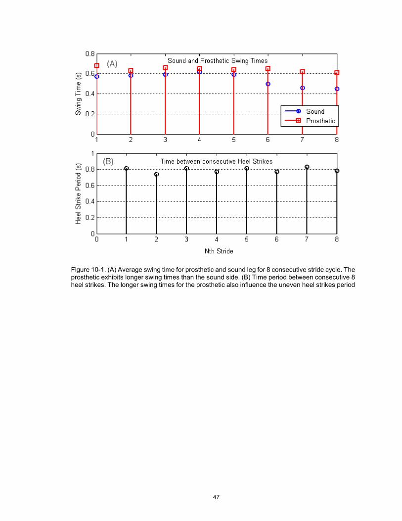
The first response of a user walking with prototype is a decreased cadence (i.e. increase
stride period) with an increasing stride length, which is often typical of amputees. The
average stride period was found to be around 1.56 seconds, which is noticeably less than
the user walking freely on the treadmill. As the user walks with an increases stride period,
the time spent on each leg is uneven. The user generally spends longer time on his sound
leg during stance as indicated by the longer swing period of prosthetic leg (Fig 10-1).
Though, the average difference in the swing time period are about 100 ms, they are

46
representative of much improved swing times. Swing times prior to final tuning display
differences of more that 200 ms, and gait is visibly asymmetrical. The swing times were
improved upon by increasing the stiffness component of the knee joint during swing
extension to influence a faster forward swing. However, continuously strengthening the
stiffness did not result in increased swing times, since the user would hold the knee at full
extension for a while before heel strike. Thus, past some threshold period, decreasing the
forward swing period made the user vulnerable to stumbles and unnatural looking swing
behavior, while providing no significant improvement in temporal asymmetry. The sound
side leg swing time can also undergo variation as can be seen towards the latter end of the
graph (Fig 10-1) as is most likely a response to a non-ideal stance behavior on the
prosthetic side. Ultimately the asymmetry in swing times is likely due to the distinctly
different inertial properties of the prosthesis and natural limb, thus a certain amount of
difference in the time period is to be expected.
47
Figure 10-1. (A) Average swing time for prosthetic and sound leg for 8 consecutive stride cycle. The prosthetic exhibits longer swing times than the sound side. (B) Time period between consecutive 8 heel strikes. The longer swing times for the prosthetic also influence the uneven heel strikes period
48
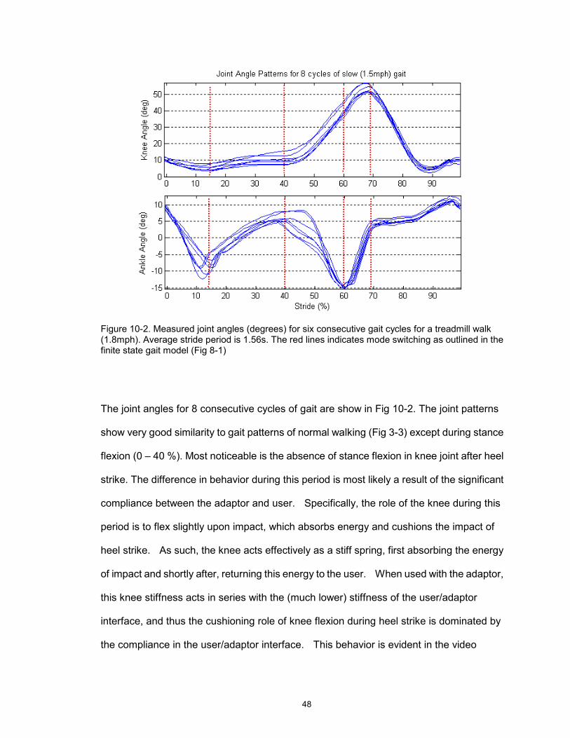
Figure 10-2. Measured joint angles (degrees) for six consecutive gait cycles for a treadmill walk (1.8mph). Average stride period is 1.56s. The red lines indicates mode switching as outlined in the finite state gait model (Fig 8-1)
The joint angles for 8 consecutive cycles of gait are show in Fig 10-2. The joint patterns
show very good similarity to gait patterns of normal walking (Fig 3-3) except during stance
flexion (0 – 40 %). Most noticeable is the absence of stance flexion in knee joint after heel
strike. The difference in behavior during this period is most likely a result of the significant
compliance between the adaptor and user. Specifically, the role of the knee during this
period is to flex slightly upon impact, which absorbs energy and cushions the impact of
heel strike. As such, the knee acts effectively as a stiff spring, first absorbing the energy
of impact and shortly after, returning this energy to the user. When used with the adaptor,
this knee stiffness acts in series with the (much lower) stiffness of the user/adaptor
interface, and thus the cushioning role of knee flexion during heel strike is dominated by
the compliance in the user/adaptor interface. This behavior is evident in the video

49
recordings of the gait trials by watching the relative motion between the top of the brace
and the subject’s hip during heel strike. Once the axial compliance between the user and
prosthesis is reduced significantly (as would be the case with an amputee subject), the
knee joint is likely to exhibit the flexion and subsequent extension evidenced in the
prototypical gait kinematics of Fig. 3-6.
Beside stance flexion-extension, the joint patterns are reasonably close to normal
biomechanical patterns. The swing flexion is slightly lower than normal values; however
this was to be expected due to issues of back drivability in the actuators and did not
interfere significantly with gait. The ankle flexed past 5 degrees prior to undergoing an
impulsive extension to provide push off.
A relatively harder task was to tune the knee and ankle joint to coordinate toe-off. During
Toe off, the ankle goes through rapid extension to provide an impulsive push, while the
knee simultaneously flexes to avoid any jerks in the body due to the extension of the
ankle. It was found to be particularly beneficial to tune the ankle first during this phase, to
ensure proper interaction with the ground to generate necessary torques. Once, the ankle
was tuned to generate the desired ankle torque with in a set amount of range of ankle
extension, the knee stiffness was then tuned to enable a certain amount of correlated
flexion in the knee. The standard ratio of knee to ankle angle during push off was found to
be between 1.2 – 1.4 through population data [1], and the measured average ratio for the
trial was 1.2. The ratio of knee to ankle angle was found to be a useful measure of position
interaction between the joints during toe off.

50
Figure 10-3. Measured joint torques (N.m) for eight consecutive gait cycles for a treadmill walk (1.8mph). Average stride period is 1.56s. The red lines indicate mode switching as outlined in the finite state gait model (Fig 23)
Figure 10-4. Average Joint Power for eight consecutive gait cycles for a treadmill walk (1.8mph). Average stride period is 1.56s. Red indicates positive power output and blue the negative power dissipation

51
The measured joint torques (Fig 10-3) during the gait show high cycle-to-cycle variability
during the stance flexion mode (0 – 40 %), which as discussed earlier is likely due to the
compliant interaction between the adapter brace and the user. The torque levels for the
rest of the modes for both knee and ankle compare quite well to average population data
(Fig 5-1). Sharp transition due to certain transitions behavior can be seen in the torque
profile, however, they are too small to noticeably affect the user. In fact, the tuning of
parameters is also done in such a manner that the transition between modes do not result
in significantly high ‘step’ in forces.
The knee and ankle joint powers, which were computed directly from the torque and
differentiated angle data, are shown in Fig. 10-4, and indicate that the prosthesis is
supplying a significant amount of power to the user. As discussed earlier, a small positive
push is provided during swing (70% of stride) to improve symmetry of swing times
between the sound and prosthetic side. The large damping behavior of the knee joint
during swing is also very apparent. However, the noticeable feature is the large power
output at the ankle joint during push off. Note that the measured power compares
favorably to that measured for healthy subjects (Fig 1-1), and thus indicates an enhanced
level of functionality relative to existing passive prostheses
The final set of tuned impedance parameters for the knee and ankle joint in each mode are
listed in Table 10-1.
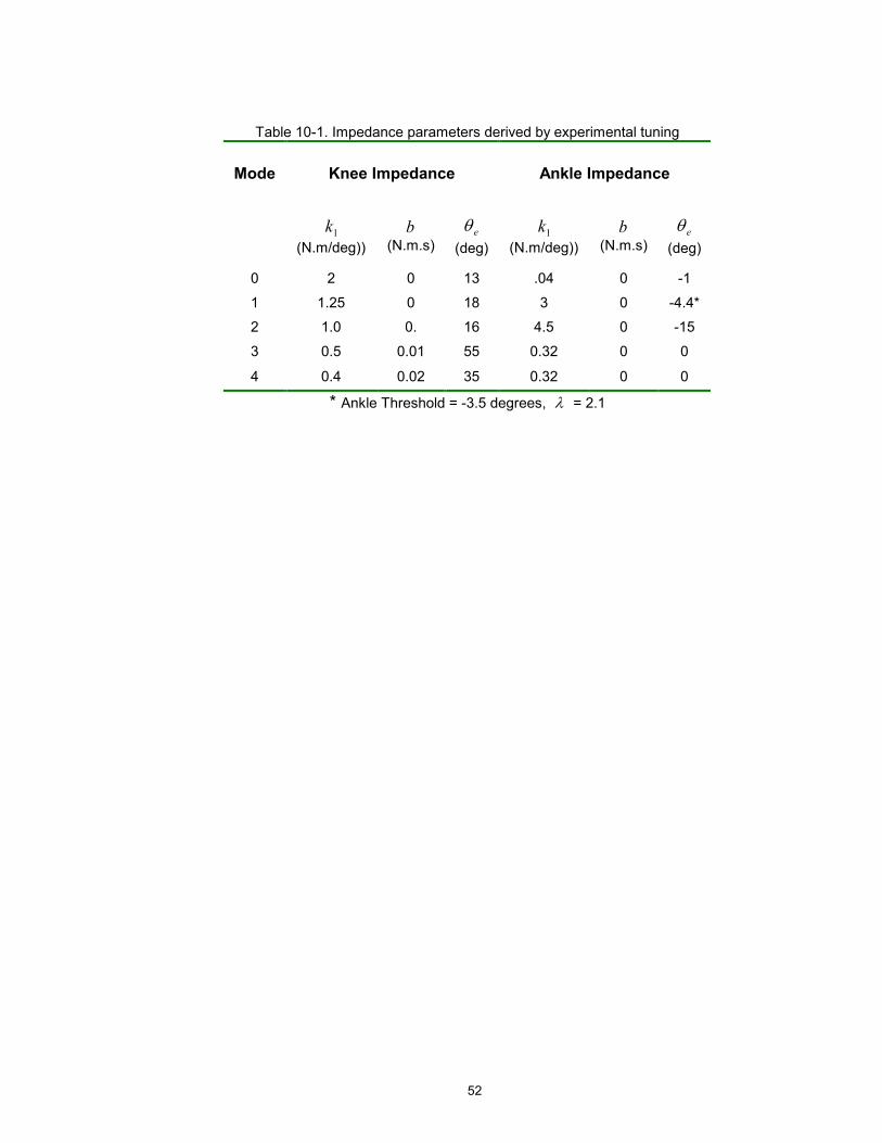
52
Table 10-1. Impedance parameters derived by experimental tuning
Mode Knee Impedance Ankle Impedance
1k
(N.m/deg))
b
(N.m.s) e
θ
(deg) 1k
(N.m/deg))
b
(N.m.s) e
θ
(deg)
0 2 0 13 .04 0 -1
1 1.25 0 18 3 0 -4.4*
2 1.0 0. 16 4.5 0 -15
3 0.5 0.01 55 0.32 0 0
4 0.4 0.02 35 0.32 0 0
* Ankle Threshold = -3.5 degrees, λ = 2.1

53
CHAPTER XI
CONCLUSIONS
A number of opportunities and challenges lie ahead towards the realization of functional
powered transfemoral prosthesis. This project has explored a possible avenue of an
impedance based control framework that allows for the generation of torques at the
prosthetic joints in a stable manner. Gait trials with an able bodied adapter was validated
against population gait data and the method has demonstrated sufficient strength to
further explore its feasibility. However, further improvement of the control framework will
have to go hand in hand with refinements of hardware and test setup. The able-bodied
adapter provides a useful setup for preliminary testing of the control architecture, though
further enhancements will need to be made to achieve greater realism in simulating
normal gait. Higher output impedance at the joint due to non-back drivability of the
pneumatic actuator also presents a significant challenge, which could partly be addressed
by improving upon the valve mechanism. The overall control could benefit from improved
valve bandwidth and reduced lag in the air supply; and changes are already underway to
address these issues.
Regarding the controller, several further improvements are necessary. A reliable
quantitative method of evaluating gait with an improved sensor set is the foremost of
challenges and one that could significantly improve the ability to deliver better results.
Moving towards partial or full automation of tuning of impedance model parameters could
significantly reduce rehabilitation and testing times. This is likely to require a broader
understanding of the variation in parameters with different gait speed. The impedance

54
model could be further expanded to cover steps and ramp walking to improve
functionality. Ultimately, the controller is likely to be used in conjunction with an intelligent
user intent recognition system to deliver a complete set of locomotive functionality to an
amputee.
Finally, the incredible versatility that human show in adapting and coordinating with
external devices is demonstrated. If the prosthesis are designed to suitably approximate
normal limb dynamics with sufficient power, than humans have the capability to leverage it
effectively to aid locomotion. We hope to further pursue the design and control frame work
for powered prosthetic technology through this perspective

55
APPENDIX A: CONSTRAINED PIECEWISE FITTING OF KNEE AND ANKLE
TORQUES DURING NORMAL SPEED LEVEL WALK
Matlab code for “Constrained Piecewise fitting of knee and ankle torques during normal
speed level walk” to data Provided by Winter [1]
%Piecewise constrained fitting of gait data to impedance model %(Linear Spring + Damper) clear %Load desired Winter, cadence data load('../../Winter Data/normal_cadence_data.mat'); %Estimated mass of user to use with normalized data mass = 75; %Display splined Winter reported knee and ankle torque, %for a complete stride cycle figure m = mass; subplot(2,1,1); xx = 0:0.1:100; yy = spline(stride,-m.*knee_torque,xx); plot(xx,yy,'LineWidth',2); hold on subplot(2,1,2); yy = spline(stride,-m.*ankle_torque,xx); plot(xx,yy,'LineWidth',2); hold on; %Specify Partition of a stride cycle into four modes %range1 = 1:19;range2 = 20:32; range3 = 33:37; range4 = 38:51; %The following specifies the array index for the desired %paritition range in pairs, eg. the following partitions the %gait into 0-42%, 44-66%, and so on ranges = [1 22 23 31 32 37 38 51]; %Temporarily set mass to '1' so as to use the Winter nomalized data %directly m = 1; %Array to store parameter and output of constrained LS fit KneefitYY = []; Kneeparams = []; AnklefitYY = []; Ankleparams = [];

56
%Array to store ratio of stiffness to damping terms predicted by fit KneeRatio = []; AnkleRatio = []; %Store equillibrium angle for knee and ankle spring KneeTheta = 0; AnkleTheta = 0; k=1; %Iterate through each partition specified in the range... for (i = 1:2:length(ranges)) %Current range range = (ranges(i)):(ranges(i+1));
%For each iteration find a suitable equilibrium point, that minimizes
%the standard deviation measure. KstdMeasure = 100; AstdMeasure = 100; %Specify settings for the constrained fitting. opt = optimset('Display','off','TolFun',1e-8,'TolX',1e-7);
%Iterate through a reasonable range of theta to find an optimal value
for (theta = -50:1:100) %%%%%Fit Knee torques%%%%%%%%% %Setup X & Y variables for LS fitting for knee KXX = -1.*[(knee_angle(range)-theta) knee_vel(range)]; KYY = (-m.*knee_torque(range)); %Constrained non-negative Least Squares (LS) fitting kb = lsqnonneg(KXX,KYY,1e-3.*[5;0],opt); %%%%%Fit Ankle torques%%%%%%%%% %Setup X & Y variables for LS fitting for ankle AXX = -1.*[(ankle_angle(range)-theta) ankle_vel(range)]; AYY = (-m.*ankle_torque(range)); %Constrained non-negative Least Squares (LS) fitting ab = lsqnonneg(AXX,AYY,1e-3.*[5;0],opt); %Calculate the Mean Square of the error residual AnkleFitError = sum((AYY-AXX*ab).^2); KneeFitError = sum((KYY-KXX*kb).^2); %Compare if this choice of equillibrium theta provides a smaller %error residual, if it does store it as the optimal theta if (KneeFitError < KstdMeasure) KstdMeasure = KneeFitError; KneeTheta = theta; end if (AnkleFitError < AstdMeasure) AstdMeasure = AnkleFitError; AnkleTheta = theta; end end %End search for optimal equilibrium theta

57
%Use the optimal equillibrium angle to performed LS fit KX1 = -1.*[(knee_angle(range)-KneeTheta) knee_vel(range)]; AX1 = -1.*[(ankle_angle(range)-AnkleTheta) ankle_vel(range)]; KY1 = [-m.*knee_torque(range)]; AY1 = [-m.*ankle_torque(range)]; %Find best fit using constrained least squares %Fitting is sensitive to choice of initial conditions kb1 = lsqnonneg(KX1,KY1,1e-3.*[5;0],opt); ab1 = lsqnonneg(AX1,AY1,1e-3.*[5;0],opt); %Determining the contribution of stiffness and damping terms %For Knee KY = KX1*kb1; kd_contbn = kb1(2).*knee_vel(range); %Damping contribution ks_contbn = KY-kd_contbn; %Stiffness contribution %Ratio of stiffness to damping contribution k_ratio(k) = mean(abs(ks_contbn./kd_contbn)); %For Ankle AY = AX1*ab1; ad_contbn = ab1(2).*ankle_vel(range); %Damping contribution as_contbn = AY-ad_contbn; %Stiffness contribution %Ratio of stiffness to damping contribution a_ratio(k) = mean(abs(as_contbn./ad_contbn)); %Store output predicted from constrained LS fitting KneefitYY = [KneefitYY; KX1*kb1]; AnklefitYY = [AnklefitYY; AX1*ab1]; %Store Impedance parameters for this stride partition kb1(4) = KneeTheta; Kneeparams = [Kneeparams kb1]; ab1(4) = AnkleTheta; Ankleparams = [Ankleparams ab1]; %Plot Vertical Lines indicating partition boundary of stride m = mass; subplot(2,1,1); %plot(stride(range),m.*KX1*kb1(1:3),'--g','LineWidth',3); plot([stride(range(end)) stride(range(end))],m.*[-1 0.5],'--r','LineWidth',1) %text(stride(range(3)),-.75,num2str(k_ratio(k),3)); subplot(2,1,2); hold on %plot(stride(range),m.*AX1*ab1(1:3),'--g','LineWidth',3) plot([stride(range(end)) stride(range(end))],m.*[-2 1],'--r','LineWidth',1) %text(stride(range(3)),-1.5,num2str(a_ratio(k),3)) m = 1; k=k+1; end

58
m = mass; %To avoid sharp jumps at the transition boundaries, %the entire output of the fitted model is splined together %and plotted subplot(2,1,1); title('Impedance fit of Knee and Ankle Joint : Linear spring + Damper'); X = stride(ranges(1):ranges(end)); Y = KneefitYY.*m; xx = 0:1:100; yy = spline(X,Y,xx); plot(xx,yy,':r','LineWidth',3); ylabel('Joint Torque'); subplot(2,1,2); X = stride(ranges(1):ranges(end)); Y = AnklefitYY.*m; xx = 0:1:100; yy = spline(X,Y,xx); plot(xx,yy,':r','LineWidth',3); xlabel('Percent of Stride'); disp('KNEE'); disp([' K1 K2 b ThetaO']) disp(Kneeparams'); disp('ANKLE'); disp([' K1 K2 b ThetaO']) disp(Ankleparams');

59
APPENDIX B.SIMULINK IMPLEMENTATION OF THE CONTROLLER TOGETHER W
ITH THE FINITE STATE MODEL

60

61

62

63

64

65

66

67

68

69

70

71
REFERENCES
[1] Winter, D.A., “The biomechanics and motor control of human gait: normal, elderly and pathological,” University of Waterloo Press, 2nd ed., 1991
[2] Winter, D. A. and Sienko, S. E., “Biomechanics of below-knee amputee gait,” J. Biomechanics. 21, 361–367., 1988.
[3] Nadeau, S., McFadyen, B.J., and Malouin, F., “Frontal and sagittal plane analyses of the stair climbing task in healthy adults aged over 40 years: What are the challenges compared to level walking?,” Clinical Biomechanics, vol. 18, no. 10, pp. 950-959., 2003.
[4] Riener, R., Rabuffetti, M., and Frigo, C., “Joint powers in stair climbing at different slopes.”, Proceedings of the IEEE International Conference on Engineering in Medicine and Biology, vol. 1, p. 530., 1999.
[5] Prilutsky, B.I., Petrova, L.N., and Raitsin, L.M., “Comparison of mechanical energy
expenditure of joint moments and muscle forces during human locomotion,” Journal of Biomechanics, vol. 29, no. 4, pp. 405-415, 1996.
[6] DeVita, P., Torry M., Glover, K.L., and Speroni, D.L.,“A Functional Knee Brace Alters
Joint Torque and Power Patterns during Walking and Running,” Journal of Biomechanics, vol. 29, no. 5, pp. 583-588, 1996.
[7] Nagano, A., Ishige, Y., and Fukashiro, S., “Comparison of new approaches to estimate
mechanical output of individual joints in vertical jumps,” Journal of Biomechanics, vol. 31, no. 10, pp. 951-955, 1998.
[8] Waters, R., Perry, J., Antonelli, D., and Hislop, H. “Energy cost of walking amputees:
the influence of level of amputation,” J. Bone and Joint Surgery. 58A, 42–46,1976 [9] Goldfarb, M., Barth, E.J., Gogola, M.A. and Wehrmeyer, J.A. “Design and Energetic
Characterization of a Liquid-Propellant-Powered Actuator for Self-Powered Robots,” IEEE/ASME Transactions on Mechatronics, vol. 8, no. 2, pp. 254-262, 2003
[10] Shields, B., and Goldfarb, M., “Design and Energetic Characterization of a Solenoid
Injected Liquid Monopropellant Powered Actuator for Self-Powered Robots,” accepted for the 2005 IEEE International Conference on Robotics and Automation, 2005
[11] Shields, B., Fite, K., and Goldfarb, M. “Control of a Direct Injection Liquid Fueled
Actuator,” Proceedings of the ASME International Mechanical Engineering Congress and Exposition, IMECE2004-59442, 2004
[12] Fite, K.B., Mitchell, J., Barth, E.J., and Goldfarb, M. “Sliding Mode Control of a
Direct-Injection Monopropellant-Powered Arm,” American Control Conference, pp. 4461-4466, 2004

72
[13] Flowers, W.C., “A Man-Interactive Simulator System for Above-Knee Prosthetics Studies,” Department of Mechanical Engineering PhD Thesis, MIT, 1973
[14] Donath, M., “Proportional EMG Control for Above-Knee Prosthesis,” Department of
Mechanical Engineering Masters Thesis, MIT, 1974 [15] Grimes, D. L. An Active Multi-Mode Above Knee Prosthesis Controller. Department of
Mechanical Engineering PhD Thesis, MIT, 1979 [16] Grimes, D. L., Flowers, W. C., and Donath, M. “Feasibility of an active control scheme
for above knee prostheses,” ASME Journal of Biomechanical Engineering, vol. 99, no. 4, pp. 215-221, 1977
[17] Stein, J.L. Design Issues in the Stance Phase Control of Above-Knee Prostheses.
Department of Mechanical Engineering PhD Thesis, MIT, 1983 [18] Stein, J.L., and Flowers, W.C. “Stance phase control of above-knee prostheses: knee
control versus SACH foot design,” Journal of Biomechanics, vol. 20, no. 1, pp. 19-28, 1987
[19] Flowers, W.C., and Mann, R.W. “Electrohydraulic knee-torque controller for a
prosthesis simulator,” ASME Journal of Biomechanical Engineering, vol. 99, no. 4, pp. 3-8, 1977
[20] Popovic, D. and Schwirtlich, L. “Belgrade active A/K prosthesis, in de Vries,” J. (Ed.),
Electrophysiological Kinesiology, Interm. Congress Ser. No. 804, Excerpta Medica, Amsterdam, The Netherlands, pp. 337–343, 1988
[21] D Popovic, R Tomovic, D Tepavac, L Schwirtlich. “Control aspects of
active-above-knee prosthesis” Volume 35 , Issue 6, pp 751 – 767, 1991 [22] Popovic D, Oguztoreli MN, Stein RB., “Optimal control for an above-knee prosthesis
with two degrees of freedom,” Journal of Biomechanics, vol. 28, no. 1, pp. 89-98, 1995 [23] Klute, G.K., Czerniecki, J., Hannaford, B., “Development of Powered Prosthetic
Lower Limb”, Proceedings of the First National Meeting, Veterans Affairs Rehabilitation Research and Development Service, 1998
[24] Klute, G.K., Czerniecki, J., Hannaford, B., “Muscle-Like Pneumatic Actuators for
Below-Knee Prostheses”, Proceedings the Seventh International Conference on New Actuators, pp. 289-292, 2000
[25] Au, S. Bonato, P., Herr, H. “An EMG-Position Controlled System for an Active
Ankle-Foot Prothesis: An Initial Experimental Study,” Proceedings of the IEEE Int Conf. On Rehabilitation Robotics, pp. 375-379, 2005
[26] Bar, A., Ishai, G., Meretsky, P. and Koren, Y. “Adaptive microcomputer control of an
artificial knee in level walking,” J. Biomed. Eng., Vol. 5, 1983 [27] Goldfarb, M, “Control for a Self-Contained Microcomputer Controlled Above-Knee
Prosthesis,” Department of Mechanical Engineering Masters Thesis, MIT, 1992

73
[28] Herr, H., and Wilkenfeld, A. “User-adaptive control of a magnetorheological prosthetic
knee,” Industrial Robot: An International Journal, 30: 42-55, 2003 [29] Jung-Hoon Kim and Jun-Ho Oh, “Development of an Above Knee Prosthesis using
MR Damper and Leg Simulator”. International Conference on Robotics 8 Automation , pp 3686-3691, 2001
[30] Mochon, S., and McMahon, T.A, “Ballistic Walking,” Journal of Biomechanics, vol. 13,
no. 1, pp. 49-57, 1980 [31] Winter, D.A “Overall principle of lower limb support during stance phase of gait”.
Journal of Biomechanics, vol. 13, no. 11, pp. 923-7, 1980 [32] Jessica Rose, James G. Gamble, “Human Walking”. Williams & Wilkins, Baltimore,
2nd Edition, 1994 [33] Inman, VT, Ralston, HJ and Todd, Frank, “Human Walking”. Williams & Wilkins,
Baltiimore, 1981 [34] Winter, D.A. “The biomechanics and motor control of human gait” University of
Waterloo Press, 2nd ed., 1991 [35] Goldberg SR, Ounpuu S, Delp SL, “The importance of swing-phase initial
conditions in stiff-knee gait,” Journal of Biomechanics, vol. 36, no. 8, pp. 1111-6, 2003 [36] Hogan, N., “Impedance Control: An Approach to Manipulation -A Three Part Paper,”
ASME Journal of Dynamic Systems, Measurement, and Control, Vol. 107, pp. 1-24, 1985
[37] Saleh, Michael and Murdoch, George. “In defense of gait analysis”. The J of Bone and
Joint surgery. Vol 67 B No 2 March 1985 [38] Gard, Steve. “Use of Quantitative Gait Analysis for the Evaluation of prosthetic
walking performance,” J of Prosthetic and Orthotics Vol 18, Num 1S p93, 2005 [39] Murray MP, Sepic SB, Gardner GM, Mollinger LA. “Gait patterns in above-knee
amputees using constant-friction components,” Bulletin for Prosthetic Research, 10-34: 35-45, 1980
[40] MOE-NILSSEN Rolf, HELBOSTAD Jorunn L. “Estimation of gait cycle characteristics
by trunk accelerometry,” Journal of biomechanics, vol. 37, no 1, pp. 121-126, 2004 [41] Sup, Frank, “Design and Control of a Powered TransFemoral Prosthesis” Department
of Mechanical Engineering, Vanderbilt University. Masters Thesis 2006