finite mathematics for the managerial, life, and social ... ·...
TRANSCRIPT

Instructions for Solving Examples and Exercises in Soo Tan’s
Finite Mathematics for the Managerial, Life,and Social Sciences, Tenth Edition
Using Microsoft Excel 2007In the examples and exercises that follow, we assume that you are familiar with the basic features of Microsoft Excel. Pleaseconsult your Excel manual or use Excel’s Help features to answer questions regarding the standard commands and operatinginstructions for Excel.
Boldfaced words/characters enclosed in a box (for example, Enter ) indicate that an action (click, select, or press) isrequired. Words/characters printed blue (for example, Chart Type) indicate words/characters that appear on the screen.Words/characters printed in a typewriter font (for example, =(-2/3)*A2+2) indicate words/characters that need to betyped and entered.
1c°2013 Cengage Learning. All Rights Reserved. May not be scanned, copied or duplicated, or posted to a publicly accessible website, in whole or in part.

Section 1.2 (p. 24)
EXAMPLE 3 Plot the graph of the straight line 2x+ 3y − 6 = 0 over the interval [−10, 10].
Solution1. Write the equation in the slope-intercept form:
y = −23x+ 2
2. Create a table of values. First, enter the input values: Enter the values of the endpoints of the interval over which youare graphing the straight line. (Recall that we need only two distinct data points to draw the graph of a straight line. Ingeneral,we select the endpoints of the interval over which the straight line is to be drawn as our data points.) In this case,we enter -10 in cell B1 and 10 in cell C1.
Second, enter the formula for computing the y-values: Here we enter= -(2/3)*B1+2
in cell B2 and then press Enter .Third, evaluate the function at the other input value: To extend the formula to cell C2, move the pointer to the small
black box at the lower right corner of cell B2 (the cell containing the formula). Observe that the pointer now appears asa black + (plus sign). Drag this pointer through cell C2 and then release it. The y-value, −4.66667, corresponding tothe x-value in cell C1 (10) will appear in cell C2 (Figure T3).
A B C1 x -10 102 y 8.666667 -4.66667
FIGURE T3Table of values for x and y
3. Graph the straight line determined by these points. First, highlight the numerical values in the table. Here wehighlight cells B1:B2 and C1:C2. Next, on the Insert tab, in the Charts group, select the second chart subtype from theScatter chart type. Click on Layout 1 in the Chart Layouts group to create a chart title and axis titles. Enter y=-
(2/3)x+2 in the Chart Title field, x in the Horizontal (Value) Axis Title field, and y in the Vertical (Value) Axis Titlefield, and delete the Series 1 Legend Entry field. The resulting graph is shown in Figure T4.
‐6
‐4
‐2
0
2
4
6
8
10
‐15 ‐10 ‐5 0 5 10 15
y
x
y=‐(2/3)x+2
FIGURE T4The graph of y = −23x+ 2 over the interval [−10, 10] ¥
2c°2013 Cengage Learning. All Rights Reserved. May not be scanned, copied or duplicated, or posted to a publicly accessible website, in whole or in part.

Section 1.2 (p. 24)
If the interval over which the straight line is to be plotted is not specified, then you may have to experiment to find anappropriate interval for the x-values in your graph. For example, you might first plot the straight line over the interval[−10, 10]. If necessary you then might adjust the interval by enlarging it or reducing it to obtain a sufficiently complete viewof the line or at least the portion of the line that is of interest.
EXAMPLE 4 Plot the straight line 2x+ 3y − 30 = 0 over the intervals (a) [−10, 10] and (b) [−5, 20].Solution a and b. We first cast the equation in the slope-intercept form, obtaining y = −23x+ 10. Following the proce-dure given in Example 3, we obtain the graphs shown in Figure T5.
024681012141618
‐15 ‐10 ‐5 0 5 10 15
y
x
y=‐(2/3)x+10
‐6‐4‐20246810121416
‐10 ‐5 0 5 10 15 20 25
y
x
y=‐(2/3)x+10
(a) (b)FIGURE T5The graph of y = −23x+ 10 over the intervals (a) [−10, 10] and (b) [−5, 20]
Observe that the graph in Figure T5b includes the x- and y-intercepts. This figure certainly gives a more complete view ofthe straight line. ¥
3c°2013 Cengage Learning. All Rights Reserved. May not be scanned, copied or duplicated, or posted to a publicly accessible website, in whole or in part.

Section 1.3 (p. 38)Excel can be used to find the value of a function at a given value with minimal effort. However, to find the value of y for agiven value of x in a linear equation such as Ax+ By + C = 0, the equation must first be cast in the slope-intercept formy = mx+ b, thus revealing the desired rule f (x) = mx+ b for y as a function of x.
EXAMPLE 3 Consider the equation 2x+ 5y = 7.a. Find the value of y for x = 0, 5, and 10.b. Plot the straight line with the given equation over the interval [0, 10].
Solutiona. Since this is a linear equation, we first cast the equation in slope-intercept form:
y = −25x+
7
5
Next, we create a table of values (Figure T3), following the same procedure outlined in Example 3 on page 2 of thisdocument. In this case we use the formula =(-2/5)*B1+7/5 for the first y-value.
A B C D1 x 0 5 102 y 1.4 -0.6 -2.6
FIGURE T3Table of values for x and y
b. Following the procedure outlined in Example 3 on page 2 of this document, we obtain the graph shown in Figure T4.
‐3
‐2.5
‐2
‐1.5
‐1
‐0.5
0
0.5
1
1.5
2
0 2 4 6 8 10 12y
x
y=‐(2/5)x+7/5
FIGURE T4The graph of y = −25x+ 7
5 over the interval [0, 10] ¥
4c°2013 Cengage Learning. All Rights Reserved. May not be scanned, copied or duplicated, or posted to a publicly accessible website, in whole or in part.

Section 1.3 (p. 38)
APPLIED EXAMPLE 4 Market for Cholesterol-Reducing Drugs In a study conducted in early 2000, experts pro-jected a rise in the market for cholesterol-reducing drugs. The U.S. market (in billions of dollars) for such drugs from 1999through 2004 is approximated by
M (t) = 1.95t+ 12.19
where t is measured in years, with t0 corresponding to 1999.a. Plot the graph of the function M over the interval [0, 6].b. Assuming that the projection held and the trend continued, what was the market for cholesterol-reducing drugs in 2005
(t = 6)?c. What was the rate of increase of the market for cholesterol-reducing drugs over the period in question?
Source: S. G. Cowen
Solutiona. Following the procedure given in Example 3 on page 2 of this document, we obtain the spreadsheet and graph shown in
Figure T5. [Note: We have made the appropriate entries for the title and x- and y-axis labels.]
A B C D1 t 0 5 62 M(t) 12.19 21.94 23.89 0
5
10
15
20
25
30
0 1 2 3 4 5 6 7
M(t) in billionsof dollars
t in years
M(t)=1.95t+12.19
(a) (b)FIGURE T5(a) The table of values for t and M (t) and(b) the graph showing the demand for cholesterol-reducing drugs
b. From the table of values, we see that
M (6) = 1.95 (6) + 12.19 = 23.89
or $23.89 billion.c. The function M is linear; hence, we see that the rate of increase of the market for cholesterol-reducing drugs is given by
the slope of the straight line represented by M , which is approximately $1.95 billion per year. ¥
5c°2013 Cengage Learning. All Rights Reserved. May not be scanned, copied or duplicated, or posted to a publicly accessible website, in whole or in part.

Section 1.5 (p. 61)Excel can be used to find an equation of the least-squares line for a set of data and to plot a scatter diagram and the least-squares line for the data.
EXAMPLE 3 Find an equation of the least-squares line for the data given in the following table:
x 1.1 2.3 3.2 4.6 5.8 6.7 8.0
y −5.8 −5.1 −4.8 −4.4 −3.7 −3.2 −2.5Plot the scatter diagram and the least-squares line for these data.
Solution1. Set up a table of values on a spreadsheet (Figure T3).
A B1 x y2 1.1 -5.83 2.3 -5.14 3.2 -4.85 4.6 -4.46 5.8 -3.77 6.7 -3.28 8 -2.5
FIGURE T3Table of values for x and y
2. Plot the scatter diagram. Highlight the numerical values in the table of values. Follow the procedure given inExample 3 on page 2 of this document, selecting the first chart subtype instead of the second from the Scatter charttype. The scatter diagram will appear.
3. Insert the least-squares line. Select the Layout tab and click on Linear Trendline in the Trendline
subgroup of the Analysis group. Then click on More Trendline Options... in the same subgroup and click on
Display Equation on chart . The equationy = 0.460x− 6.3
will appear on the chart (Figure T4).
y = 0.460x ‐ 6.3
‐7
‐6
‐5
‐4
‐3
‐2
‐1
0
0 2 4 6 8 10
y
x
Scatter diagram and least‐squares line
FIGURE T4Scatter diagram and least-squares line for the given data ¥
6c°2013 Cengage Learning. All Rights Reserved. May not be scanned, copied or duplicated, or posted to a publicly accessible website, in whole or in part.

Section 1.5 (p. 61)
Note: The following example requires the Analysis ToolPak. Use Excel’s Help function to learn how to install this add-in.
APPLIED EXAMPLE 4 Demand for Electricity According to Pacific Gas and Electric, the nation’s largest utilitycompany, the demand for electricity from 1990 through 2000 is summarized in the following table:
t 0 2 4 6 8 10
y 333 917 1500 2117 2667 3292
Here t = 0 corresponds to 1990, and y gives the amount of electricity in year t, measured in megawatts. Find an equationof the least-squares line for these data.
Solution1. Set up a table of values on a spreadsheet (Figure T5).
A B1 t y2 0 3333 2 9174 4 15005 6 21176 8 26677 10 3292
FIGURE T5Table of values for x and y
2. Find the equation of the least-squares line for the data. Click on Data Analysis in the Analysis group of the
Data tab. In the Data Analysis dialog box that appears, select Regression and then click OK . In the Regression
dialog box that appears, select the Input Y Range: box and then enter the y-values by highlighting cells B2:B7. Next
select the Input X Range: box and enter the t-values by highlighting cells A2:A7. Click OK and a SUMMARYOUTPUT worksheet will appear. In the third table, you will see the entries shown in Figure T6.
CoefficientsIntercept 328.4762X Variable 1 295.1714
FIGURE T6Entries in the SUMMARY OUTPUT worksheet
These entries give the value of the y-intercept and the coefficient of x in the equation y = mx+ b. In our example, weare using the variable t instead of x, so the required equation is
y = 328 + 295t ¥
7c°2013 Cengage Learning. All Rights Reserved. May not be scanned, copied or duplicated, or posted to a publicly accessible website, in whole or in part.

Section 2.4 (p. 113)First, we show how basic operations on matrices can be carried out using Excel.
EXAMPLE 3 Given the following matrices,
A =
⎡⎢⎢⎣1.2 3.1
−2.1 4.23.1 4.8
⎤⎥⎥⎦ and B =
⎡⎢⎢⎣4.1 3.2
1.3 6.4
1.7 0.8
⎤⎥⎥⎦a. Compute A+B. b. Compute 2.1A− 3.2B.
Solutiona. First, represent the matrices A and B in a spreadsheet (Figure T1).
A B C D E1 A B2 1.2 3.1 4.1 3.23 -2.1 4.2 1.3 6.44 3.1 4.8 1.7 0.8
FIGURE T1The elements of matrix A and matrix B in a spreadsheet
Second, compute the sum of matrix A and matrix B. Highlight the cells that will contain matrix A + B, type =,highlight the cells in matrix A, type +, highlight the cells in matrix B, and press Ctrl-Shift-Enter . The resultingmatrix A+B is shown in Figure T2.
A B8 A+B9 5.3 6.310 -0.8 10.611 4.8 5.6
FIGURE T2The matrix A+B
b. Highlight the cells that will contain matrix 2.1A − 3.2B. Type =2.1*, highlight matrix A, type -3.2*, highlight thecells in matrix B, and press Ctrl-Shift-Enter . The resulting matrix 2.1A− 3.2B is shown in Figure T3.
A B13 2.1A-3.2B14 -10.6 -3.7315 -8.57 -11.6616 1.07 7.52
FIGURE T3The matrix 2.1A− 3.2B ¥
8c°2013 Cengage Learning. All Rights Reserved. May not be scanned, copied or duplicated, or posted to a publicly accessible website, in whole or in part.

Section 2.4 (p. 113)
APPLIED EXAMPLE 4 John operates three gas stations at three locations I, II, and III. Over 2 consecutive days, his gasstations recorded the following fuel sales (in gallons):
Day 1Regular Regular Plus Premium Diesel
Location I 1400 1200 1100 200
Location II 1600 900 1200 300
Location III 1200 1500 800 500
Day 2Regular Regular Plus Premium Diesel
Location I 1000 900 800 150
Location II 1800 1200 1100 250
Location III 800 1000 700 400
Find a matrix representing the total fuel sales at John’s gas stations.
Solution The fuel sales can be represented by the matrices A (day 1) and B (day 2):
A =
⎡⎢⎢⎣1400 1200 1100 200
1600 900 1200 300
1200 1500 800 500
⎤⎥⎥⎦ and B =
⎡⎢⎢⎣1000 900 800 150
1800 1200 1100 250
800 1000 700 400
⎤⎥⎥⎦We first enter the elements of the matrices A and B onto a spreadsheet. Next, we highlight the cells that will contain the
matrix A + B, type =, highlight A, type +,highlight B, and then press Ctrl-Shift-Enter . The resulting matrix AB isshown in Figure T4.
A B C D23 A+B24 2400 2100 1900 35025 3400 2100 2300 55026 2000 2500 1500 900
FIGURE T4The matrix A+B ¥
9c°2013 Cengage Learning. All Rights Reserved. May not be scanned, copied or duplicated, or posted to a publicly accessible website, in whole or in part.

Section 2.5 (p. 128)
We use the MMULT function in Excel to perform matrix multiplication.
EXAMPLE 2 Let
A =
"1.2 3.1 −1.42.7 4.2 3.4
#B =
"0.8 1.2 3.7
6.2 −0.4 3.3
#C =
⎡⎢⎢⎣1.2 2.1 1.3
4.2 −1.2 0.61.4 3.2 0.7
⎤⎥⎥⎦
Find (a) AC and (b) (1.1A+ 2.3B)C.
Solutiona. First, enter the matrices A, B, and C into a spreadsheet (Figure T1).
A B C D E F G1 A B2 1.2 3.1 -1.4 0.8 1.2 3.73 2.7 4.2 3.4 6.2 -0.4 3.345 C6 1.2 2.1 1.37 4.2 -1.2 0.68 1.4 3.2 0.7
FIGURE T1Spreadsheet showing the matrices A, B, and C
Second, compute AC. Highlight the cells that will contain the matrix product AC, which has order 2 × 3. Type=MMULT(, highlight the cells in matrix A, type ,, highlight the cells in matrix C, type ), and press Ctrl-Shift-Enter .The matrix product AC shown in Figure T2 will appear on your spreadsheet.
A B C10 AC11 12.5 -5.68 2.4412 25.64 11.51 8.41
FIGURE T2The matrix product AC
10c°2013 Cengage Learning. All Rights Reserved. May not be scanned, copied or duplicated, or posted to a publicly accessible website, in whole or in part.

Section 2.5 (p. 128)
b. Compute (1.1A+ 2.3B)C. Highlight the cells that will contain the matrix product (1.1A+ 2.3B)C. Next, type=MMULT(1.1*, highlight the cells in matrix A, type +2.3*, highlight the cells in matrix B, type ,, highlight thecells in matrix C, type ), and press Ctrl-Shift-Enter . The matrix product shown in Figure T3 will appear in yourspreadsheet.
A B C13 (1.1A+2.3B)C14 39.464 21.536 12.68915 52.078 67.999 32.55
FIGURE T3The matrix product (1.1A+ 2.3B)C ¥
11c°2013 Cengage Learning. All Rights Reserved. May not be scanned, copied or duplicated, or posted to a publicly accessible website, in whole or in part.
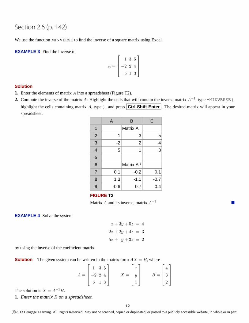
Section 2.6 (p. 142)
We use the function MINVERSE to find the inverse of a square matrix using Excel.
EXAMPLE 3 Find the inverse of
A =
⎡⎢⎢⎣1 3 5
−2 2 45 1 3
⎤⎥⎥⎦Solution1. Enter the elements of matrix A into a spreadsheet (Figure T2).2. Compute the inverse of the matrix A: Highlight the cells that will contain the inverse matrix A−1, type =MINVERSE(,
highlight the cells containing matrix A, type ), and press Ctrl-Shift-Enter . The desired matrix will appear in yourspreadsheet.
A B C1 Matrix A2 1 3 53 -2 2 44 5 1 356 Matrix A-1
7 0.1 -0.2 0.18 1.3 -1.1 -0.79 -0.6 0.7 0.4
FIGURE T2Matrix A and its inverse, matrix A−1 ¥
EXAMPLE 4 Solve the system
x+ 3y + 5z = 4
−2x+ 2y + 4z = 3
5x+ y + 3z = 2
by using the inverse of the coefficient matrix.
Solution The given system can be written in the matrix form AX = B, where
A =
⎡⎢⎢⎣1 3 5
−2 2 45 1 3
⎤⎥⎥⎦ X =
⎡⎢⎢⎣x
y
z
⎤⎥⎥⎦ B =
⎡⎢⎢⎣4
3
2
⎤⎥⎥⎦The solution is X = A−1B.1. Enter the matrix B on a spreadsheet.
12c°2013 Cengage Learning. All Rights Reserved. May not be scanned, copied or duplicated, or posted to a publicly accessible website, in whole or in part.

Section 2.6 (p. 142)
2. Compute A−1B. Highlight the cells that will contain the matrix X, and then type =MMULT(, highlight the cells in thematrix A−1, type ,, highlight the cells in the matrix B, type ), and press Ctrl-Shift-Enter . (Note: The matrix A−1
was found in Example 3.) The matrix X shown in Figure T3 will appear on your spreadsheet. Thus, x = 0, y = 0.5, andz = 0.5.
A12 Matrix X13 5.55112E-1714 0.515 0.5
FIGURE T3Matrix X gives the solution to the problem. ¥
13c°2013 Cengage Learning. All Rights Reserved. May not be scanned, copied or duplicated, or posted to a publicly accessible website, in whole or in part.

Section 2.7 (p. 151)
Here we show how to solve a problem involving a Leontief input-output model using matrix operations on a spreadsheet.
APPLIED EXAMPLE 2 Suppose that the input-output matrix associated with an economy is given by matrix A and thatthe matrix D is a demand vector, where
A =
⎡⎢⎢⎣0.2 0.4 0.15
0.3 0.1 0.4
0.25 0.4 0.2
⎤⎥⎥⎦ and D =
⎡⎢⎢⎣20
15
40
⎤⎥⎥⎦Find the final outputs of each industry such that the demands of industry and the consumer sector are met.
Solution1. Enter the elements of the matrices A and D onto a spreadsheet (Figure T1).
A B C D E1 Matrix A Matrix D2 0.2 0.4 0.15 203 0.3 0.1 0.4 154 0.25 0.4 0.2 40
FIGURE T1Spreadsheet showing matrix A and matrix D
2. Find (I −A)−1. Enter the elements of the 3 × 3 identity matrix I onto a spreadsheet. Highlight the cells that willcontain the matrix (I −A)−1. Type =MINVERSE(, highlight the cells containing the matrix I; type -, highlight thecells containing the matrix A; type ), and press Ctrl-Shift-Enter . These results are shown in Figure T2.
A B C6 Matrix I7 1 0 08 0 1 09 0 0 11011 Matrix (I-A)-1
12 2.151777 1.460134 1.13352513 1.306436 2.315082 1.40249814 1.325648 1.613833 2.305476
FIGURE T2Matrix I and matrix (I −A)−1
14c°2013 Cengage Learning. All Rights Reserved. May not be scanned, copied or duplicated, or posted to a publicly accessible website, in whole or in part.

Section 2.7 (p. 151)
3. Compute (I −A)−1 *D. Highlight the cells that will contain the matrix (I −A)−1 *D. Type =MMULT(, highlightthe cells containing the matrix (I −A)−1, type ,, highlight the cells containing the matrix D, type ), and press
Ctrl-Shift-Enter . The resulting matrix is shown in Figure T3. So, the final outputs of the first, second, and thirdindustries are 110.28, 116.95, and 142.94, respectively.
A16 Matrix (I-A)-1*D17 110.278618 116.954919 142.9395
FIGURE T3Matrix (I −A)−1 *D ¥
15c°2013 Cengage Learning. All Rights Reserved. May not be scanned, copied or duplicated, or posted to a publicly accessible website, in whole or in part.

Section 4.1 (p. 228)Solver is an Excel add-in that is used to solve linear programming problems. When you start the Excel program, checkthe Data tab for the Solver tool in the Analysis group. If it is not there, you will need to install it. (Check your manual forinstallation instructions.)
EXAMPLE 2 Solve the following linear programming problem:
Maximize P = 6x+ 5y + 4z
subject to 2x+ y + z ≤ 180x+ 3y + 2z ≤ 3002x+ y + 2z ≤ 240x ≥ 0, y ≥ 0, z ≥ 0
Solution1. Enter the data for the linear programming problem onto a spreadsheet. Enter the labels shown in column A and
the variables with which we are working under Decision Variables in cells B4:B6, as shown in Figure T1. This optionalstep will help us organize our work.
A B C D E F G H I1 Maximization Problem23 Decision Variables4 x 05 y 06 z 078 Objective Function 0910 Constraints11 0 <= 18012 0 <= 30013 0 <= 240
Formulas for indicated cellsC8: = 6*C4 + 5*C5 + 4*C6C11: = 2*C4 + C5 + C6C12: = C4 + 3*C5 + 2*C6C13: = 2*C4 + C5 + 2*C6
FIGURE T1Setting up the spreadsheet for Solver
For the moment, the cells that will contain the values of the variables (C4:C6) are left blank. In C8 type the formulafor the objective function: =6*C4+5*C5+4*C6. In C11 type the formula for the left-hand side of the first constraint:=2*C4+C5+C6. In C12 type the formula for the left-hand side of the second constraint: =C4+3*C5+2*C6. In C13type the formula for the left-hand side of the third constraint: =2*C4+C5+2*C6. Zeros will then appear in cell B8 andcells C11:C13. In cells D11:D13, type <= to indicate that each constraint is of the form ≤. Finally, in cells E11:E13,type the right-hand value of each constraint—in this case, 180, 300, and 240, respectively. Note that we need not enterthe nonnegativity constraints x ≥ 0, y ≥ 0, and z ≥ 0. The resulting spreadsheet is shown in Figure T1, where theformulas that were entered for the objective function and the constraints are shown in the comment box.
16c°2013 Cengage Learning. All Rights Reserved. May not be scanned, copied or duplicated, or posted to a publicly accessible website, in whole or in part.

Section 4.1 (p. 228)
2. Use Solver to solve the problem. Under the Data tab, click on Solver in the Analysis group. The Solver Parametersdialog box will appear.a. The pointer will be in the Set Target Cell: box (refer to Figure T2). Highlight the cell on your spreadsheet containing
the formula for the objective function—in this case, C8.
FIGURE T2The completed Solver Parameters dialog box
Then, next to Equal To: select Max . Select the By Changing Cells: box and highlight the cells in your spread-
sheet that will contain the values of the variables—in this case, C4:C6. Select the Subject to the Constraints:
box and then click Add . The Add Constraint dialog box will appear (Figure T3).
FIGURE T3The Add Constraint dialog box
b. The pointer will appear in the Cell Reference: box. Highlight the cells on your spreadsheet that contain the for-mula for the left-hand side of the first constraint—in this case, C11. Next, select the symbol for the appropriateconstraint—in this case, <= . Select the box and highlight the value of the right-hand side of the first constraint on
your spreadsheet—in this case, 180. Click Add and then follow the same procedure to enter the second and third
constraints. Click OK . The resulting Solver Parameters dialog box shown in Figure T2 will appear.
17c°2013 Cengage Learning. All Rights Reserved. May not be scanned, copied or duplicated, or posted to a publicly accessible website, in whole or in part.

Section 4.1 (p. 228)
c. In the Solver Parameters dialog box, click Options (see Figure T2). In the Solver Options dialog box that appears,
select Assume Linear Model and Assume Non-Negative constraints (Figure T4). Click OK .
FIGURE T4The Solver Options dialog box
d. In the Solver Parameters dialog box that appears (see Figure T2), click Solve . A Solver Results dialog box willthen appear and at the same time the answers will appear on your spreadsheet (Figure T5).
A B C D E1 Maximization Problem23 Decision Variables4 x 485 y 846 z 078 Objective Function 708910 Constraints11 180 <= 18012 300 <= 30013 240 <= 240
FIGURE T5Completed spreadsheet after using Solver
3. Read off your answers. From the spreadsheet, we see that the objective function attains a maximum value of 708(cell C8) when x = 48, y = 84, and z = 0 (cells C4:C6). ¥
18c°2013 Cengage Learning. All Rights Reserved. May not be scanned, copied or duplicated, or posted to a publicly accessible website, in whole or in part.

Section 4.2 (p. 246)EXAMPLE 2
Minimize C = 2x+ 3y
subject to 8x+ y ≥ 80
3x+ 2y ≥ 100x+ 4y ≥ 80
x ≥ 0, y ≥ 0
Solution We use Solver as outlined in Example 2 on page 16 of this document to obtain the spreadsheet shown inFigure T1. (In this case, select Min next to Equal to: instead of Max because this is a minimization problem. Also select
>= in the Add Constraint dialog box because the inequalities in the problem are of the form≥.) From the spreadsheet, weread off the solution: x = 24, y = 14, and C = 90.
A B C D E F G H I1 Minimization Problem23 Decision Variables4 x 245 y 14678 Objective Function 90910 Constraints11 206 >= 8012 100 >= 10013 80 >= 80
Formulas for indicated cellsC8: = 2*C4 + 3*C5C11: = 8*C4 + C5C12: = 3*C4 + 2*C5C13: =C4 + 4*C5
FIGURE T1Completed spreadsheet after using Solver ¥
EXAMPLE 3 Sensitivity Analysis (for those who have completed Section 3.4) Solve the following linear program-ming problem:
Maximize P = 2x+ 4y
subject to 2x+ 5y ≤ 19 Constraint 1
3x+ 2y ≤ 12 Constraint 2
x ≥ 0, y ≥ 0a. Use Solver to solve the problem.b. Find the range of values that the coefficient of x can assume without changing the optimal solution.c. Find the range of values that Resource 1 (the constant on the right-hand side of constraint 1) can assume without changing
the optimal solution.d. Find the shadow price for Resource 1.
19c°2013 Cengage Learning. All Rights Reserved. May not be scanned, copied or duplicated, or posted to a publicly accessible website, in whole or in part.

Section 4.2 (p. 246)
e. Identify the binding and nonbinding constraints.
Solutiona. Use Solver as outlined in Example 2 on page 16 of this document to obtain the spreadsheet shown in Figure T2.
A B C D E F G H I1 Maximization Problem23 Decision Variables4 x 25 y 3678 Objective Function 16910 Constraints11 19 <= 1912 12 <= 12
Formulas for indicated cellsC8: = 2*C4 + 4*C5C11: = 2*C4 + 5*C5C12: = 3*C4 + 2*C5
FIGURE T2Completed spreadsheet for a maximization problem
b. In the Solver Results dialog box, hold down Ctrl while selecting Answer and Sensitivity under Reports, and then
click OK . By clicking the Answer Report 1 and Sensitivity Report 1 tabs that appear at the bottom of yourworksheet, you can obtain the reports shown in Figures T3a and T3b.
Target Cell (Max)
Cell Name Original Value Final Value
$C$8 Objective Function 0 16
Adjustable Cells
Cell Name Original Value Final Value
$C$4 x 0 2
$C$5 y 0 3
Constraints
Cell Name Cell Value Formula Status Slack
$C$11 19 $C$11<=$E$11 Binding 0
$C$12 12 $C$12<=$E$12 Binding 0
FIGURE T3(a) Solver’s Answer Report
20c°2013 Cengage Learning. All Rights Reserved. May not be scanned, copied or duplicated, or posted to a publicly accessible website, in whole or in part.

Section 4.2 (p. 246)
Adjustable Cells
Cell NameFinalValue
ReducedCost
ObjectiveCoefficient
AllowableIncrease
AllowableDecrease
$C$4 2 0 2 4 0.4
$C$5 3 0 4 1 2.666666667
Constraints
Cell NameFinalValue
ShadowPrice
ConstraintR.H. Side
AllowableIncrease
AllowableDecrease
$C$11 19 0.727272727 19 11 11
$C$12 12 0.181818182 12 16.5 4.4
FIGURE T3(b) Solver’s Sensitivity ReportFrom the sensitivity report, we see that the value of the Objective Coefficient for x is 2, the Allowable Increase for thecoefficient is 4, and the Allowable Decrease for the coefficient is 0.4. Thus, the coefficient can vary from 1.6 to 6withoutaffecting the optimal solution.
c. From the sensitivity report, we see that the Final Value of the constraint for resource 1 is 19 and the Allowable Increaseand Allowable Decrease for this value is 11. Thus, the value of the constraint must lie between 19−11 and 19+11—thatis, between 8 and 30.
d. From the sensitivity report, we see that the Shadow Price for resource 1 is 0.727272727.e. From the answer report, we conclude that both Constraints are binding. ¥
21c°2013 Cengage Learning. All Rights Reserved. May not be scanned, copied or duplicated, or posted to a publicly accessible website, in whole or in part.

Section 5.1 (p. 282)Excel has many built-in functions for solving problems involving the mathematics of finance. Here we illustrate the use ofthe FV (future value), EFFECT (effective rate),and the PV (present value) functions to solve problems of the type that wehave encountered in Section 5.1.
EXAMPLE 4 Finding the Accumulated Amount of an Investment Find the accumulated amount after 10 yearsif $5000 is invested at a rate of 10% per year compounded monthly.
Solution Here we are computing the future value of a lump-sum investment, so we use the FV (future value) function.
Click Financial from the Function Library on the Formulas tab and select FV . The Function Arguments dialog box willappear (see Figure T4). In our example, the mouse cursor is in the edit box headed by Type, so a definition of that termappears near the bottom of the box. Figure T4 shows the entries for each edit box in our example.
FIGURE T4Excel’s dialog box for computing the future value (FV) of an investment
Note that the entry for Nper is given by the total number of periods for which the investment earns interest. The Pmt box isleft blank since no money is added to the original investment. The Pv entry is 5000. The entry for Type is a 1 because thelump-sum payment is made at the beginning of the investment period. The answer, −$13,535.21, is shown at the bottom ofthe dialog box. It is negative because an investment is considered to be an outflow of money (money is paid out). (Click
OK and the answer will also appear on your spreadsheet.) ¥
22c°2013 Cengage Learning. All Rights Reserved. May not be scanned, copied or duplicated, or posted to a publicly accessible website, in whole or in part.

Section 5.1 (p. 282)
EXAMPLE 5 Finding the Effective Rate of Interest Find the effective rate of interest corresponding to a nominalrate of 10% per year compounded quarterly.
Solution Here we use the EFFECT function to compute the effective rate of interest. Accessing this function from theFinancial function library subgroup and making the required entries, we obtain the Function Arguments dialog box shownin Figure T5. The required effective rate is approximately 10.38% per year.
FIGURE T5Excel’s dialog box for the effective rate of interest function (EFFECT) ¥
EXAMPLE 6 Finding the Present Value of an Investment Find the present value of $20,000 due in 5 years ifthe interest rate is 7.5% per year compounded daily.
Solution We use the PV function to compute the present value of a lump-sum investment. Accessing this function asabove and making the required entries, we obtain the PV dialog box shown in Figure T6. Once again,the Pmt edit box isleft blank since no additional money is added to the original investment. The Fv entry is 20000. The answer is negativebecause an investment is considered to be an outflow of money (money is paid out). We deduce that the required amount is$13,746.32.
FIGURE T6Excel’s dialog box for the present value function (PV) ¥
23c°2013 Cengage Learning. All Rights Reserved. May not be scanned, copied or duplicated, or posted to a publicly accessible website, in whole or in part.

Section 5.2 (p. 294)Now we show how Excel can be used to solve financial problems involving annuities.
EXAMPLE 3 Finding the Future Value of an Annuity Find the amount of an ordinary annuity of 36 quarterlypayments of $220 each that earn interest at the rate of 10% per year compounded quarterly.
Solution Here we are computing the future value of a series of equal payments, so we use the FV (future value) function.As before, we choose this function from the Financial function library to obtain the Function Arguments dialog box. Aftermaking each of the required entries, we obtain the dialog box shown in Figure T3.
FIGURE T3Excel’s dialog box for the future value (FV) of an annuity
Note that a 0 is entered in the Type edit box because payments are made at the end of each payment period. Once again, theanswer is negative because cash is paid out. We deduce that the desired amount is $12,606.31. ¥
24c°2013 Cengage Learning. All Rights Reserved. May not be scanned, copied or duplicated, or posted to a publicly accessible website, in whole or in part.

Section 5.2 (p. 294)
EXAMPLE 4 Finding the Present Value of an Annuity Find the present value of an ordinary annuity consistingof 48 monthly payments of $300 each and earning interest at the rate of 9% per year compounded monthly.
Solution Here we use the PV function to compute the present value of an annuity. Accessing the PV (present value) func-tion from the Financial function library and making the required entries, we obtain the PV dialog box shown in Figure T4.We see that the required present value of the annuity is $12,055.43.
FIGURE T4Excel’s dialog box for computing the present value (PV) of an annuity ¥
25c°2013 Cengage Learning. All Rights Reserved. May not be scanned, copied or duplicated, or posted to a publicly accessible website, in whole or in part.

Section 5.3 (p. 309)Here we use Excel to help us solve problems involving amortization and sinking funds.
APPLIED EXAMPLE 3 Finding the Payment to Amortize a Loan The Wongs are considering a preapproved30-year loan of $120,000 to help finance the purchase of a house. The mortgage company charges interest at the rate of8% per year on the unpaid balance, with interest computations made at the end of each month. What will be the monthlyinstallments if the loan is amortized at the end of the term?
Solution We use the PMT function to solve this problem. Accessing this function from the Financial function librarysubgroup and making the required entries, we obtain the Function Arguments dialog box shown in Figure T3. We see thatthe desired result is $880.52. (Recall that cash you pay out is represented by a negative number.)
FIGURE T3Excel’s dialog box for giving the payment function, PMT ¥
26c°2013 Cengage Learning. All Rights Reserved. May not be scanned, copied or duplicated, or posted to a publicly accessible website, in whole or in part.

Section 5.3 (p. 309)
APPLIED EXAMPLE 4 Finding the Payment in a Sinking Fund Heidi wishes to establish a retirement accountthat will be worth $500,000 in 20 years’ time. She expects that the account will earn interest at the rate of 11% per yearcompounded monthly. What should be the monthly contribution into her account each month?
Solution As in Example 3, we use the PMT function, but this time we are given the future value of the investment.Accessing the PMT function as before and making the required entries, we obtain the Function Arguments dialog boxshown in Figure T4. We see that Heidi’s monthly contribution should be $577.61. (Note that the value for PMT is negativebecause it is an outflow.)
FIGURE T4Excel’s dialog box for giving the payment function, PMT ¥
27c°2013 Cengage Learning. All Rights Reserved. May not be scanned, copied or duplicated, or posted to a publicly accessible website, in whole or in part.

Section 6.4 (p. 358)Excel has built-in functions for calculating factorials, permutations, and combinations.
EXAMPLE 2 Use Excel to calculatea. 12!b. P (52, 5)
c. C (38, 10)
Solutiona. In cell A1, enter =FACT(12) and press Shift-Enter . The number 479001600 will appear.
b. In cell A2, enter =PERMUT(52,5) and press Shift-Enter . The number 311875200 will appear.
c. In cell A3, enter =COMBIN(38,10) and press Shift-Enter . The number 472733756 will appear.
28c°2013 Cengage Learning. All Rights Reserved. May not be scanned, copied or duplicated, or posted to a publicly accessible website, in whole or in part.

Section 8.1 (p. 437)
Excel can be used to plot the histogram for a given set of data, as illustrated by the following example.
APPLIED EXAMPLE 2 A survey of 90,000 households conducted in a certain year revealed the following percentageof women who wear a shoe size within the given ranges.
Shoe Size <5 5–512 6–612 7–712 8–812 9–912 10–1012 >1012
Women, % 1 5 15 27 29 14 7 2
Source: Footwear Market Insights survey
Let X denote the random variable taking on the values 1 through 8, where 1 corresponds to a shoe size less than 5, 2 corre-sponds to a shoe size of 5–512 , and so on.a. Plot a histogram for the given data.b. What percent of women in the survey wear a shoe size within the ranges 7–712 or 8–812 shoes?
Solutiona. Enter the given data in columns A and B onto a spreadsheet, as shown in Figure T2.
A B C1 X Frequency Probability2 1 1 0.013 2 5 0.054 3 15 0.155 4 27 0.276 5 29 0.297 6 14 0.148 7 7 0.079 8 2 0.0210 100
FIGURE T2Completed spreadsheet for Example 2
Highlight the data in column B and selectP
from the Editing group under the Home tab. The sum of the numbers in
this column (100) will appear in cell B10. In cell C2, type =B2/100 and then press Enter . To extend the formula tocell C9, select cell C2 and move the pointer to the small black box at the lower right corner of that cell. Drag the black+that appears (at the lower right corner of cell C2) through cell C9 and then release it. The probability distribution shownin cells C2 to C9 will then appear on your spreadsheet. Then highlight the data in the Probability column and selectColumn from the Charts group under the Insert tab. Click on the first chart type (Clustered Column). Under the Layouttab, click on Chart Title in the Labels group and select Centered Overlay Title . Enter Histogram as the title.
Select Primary Axis Title/Horizontal Title under Axis Titles from the Labels group and enter Probability asthe vertical axis title, and similarly enter X as the horizontal axis title. Finally, delete the Series 1 legend entry.
29c°2013 Cengage Learning. All Rights Reserved. May not be scanned, copied or duplicated, or posted to a publicly accessible website, in whole or in part.

Section 8.1 (p. 437)
The histogram will appear as shown in Figure T3.
0
0.05
0.1
0.15
0.2
0.25
0.3
0.35
1 2 3 4 5 6 7 8
Probability
X
Histogram
FIGURE T3The histogram for the random variable X
b. The probability that a woman participating in the survey wears a shoe size within the ranges 7–712 or 8–812 is given byP (X = 4) + P (X = 5) = .27 + .29 = .56
This tells us that 56% of the women wear a shoe size within the ranges 7–712 or 8–812 . ¥
30c°2013 Cengage Learning. All Rights Reserved. May not be scanned, copied or duplicated, or posted to a publicly accessible website, in whole or in part.