finite element modeling of impact strength of laser welds ... · finite element modeling of impact...

Finite element modeling of impact strength of laser welds for automotive applications

N. Kuppuswamy1, R. Schmidt2, F. Seeger1 & S. Zhang1 1DaimlerChrysler AG Stuttgart, Germany 2Institute of General Mechanics, RWTH Aachen University, Germany

Abstract

Laser welding is increasingly applied in the automotive industry to assemble sheet structures due to its efficiency and reliability. However, the numerous material and gauge combinations pose a major challenge in characterizing and understanding the crash behavior of the welded joints. Body-in-white (BIW) structures normally have numerous laser welded joints along with other kinds of joints like adhesive bonding, spot welds etc. Owing to limitations in computing time, the structures with all these kinds of joints have to be modeled with coarse finite element meshes. Simplified or substitute joint models with just one or few elements but with correct representation of geometry and stiffness of the joint are largely desired in practice. This paper will discuss such modeling techniques, including element selection, choice of material models for the weld etc. The type and dimension of the weld model is fixed and validated on experimental crash test results. An empirical relationship is then developed which covers the numerous physical effects like sheet thickness, static and dynamic strength and failure behavior of the joint. A general description of the model and some recommendations for application of the model where coarse meshes are involved for both welds and flanges are given as well. Keywords: laser welding, material and gauge combinations, crash, coarse finite element meshes, substitute joint models, element selection, material.

1 Introduction

Substantial amount of progress has been done so far to improve the crash worthiness of passenger cars. A car body typically has a huge number of welded joints. During crash it is not just the body of the car that gets deformed but also

© 2007 WIT PressWIT Transactions on The Built Environment, Vol 94, www.witpress.com, ISSN 1743-3509 (on-line)

Safety and Security Engineering II 375

doi:10.2495/SAFE070371

the joining elements. In the previous years the joining elements have been modeled as rigid elements and their failure or deformation had been ignored in the simulations. The present body-in-white crash models take into account this pitfall by modeling the joints with deformable elements. The laser weld investigated here is called as “Robscan” which stands for the combined technology of robot control and laser scanning. The finite element modeling of such weld in crash simulations will be discussed in detail. Each of the joining techniques used in commercial applications have their own history and reasons behind their use. The car industries have invested a lot of effort in the past on research on spot welded joints to join steel sheets. But with the development of laser technology, robots, scanners (fig. 1a) in the welding applications, focus is now shifting from spot welded joints to laser welded joints. Laser welding has a number of advantages. It is almost five times faster than the conventional spot welding. The whole laser welding equipment and its accessories occupy much lesser space compared to spot welding. Hence a significant cost reduction is possible [1].

Figure 1: Robscan system (a) and scanner (b).

Apart from the high welding speeds and significant reduction in workspace, from the view of weld geometry, Robscan technology is flexible to producing different complex weld geometries. Depending on the stiffness required for the application one can choose the different weld geometries (fig 1b). Typical Robscan geometries are brackets, circles or lines. In an ideal condition the strength of the weld and the width of the weld are typically controlled by the focus diameter, speed and intensity of the laser beam. Other aspects which influence the strength of weld starkly are thickness and material of the sheets, number of sheet layers etc. The size of the heat-affected zone across the weld also depends on the above-mentioned factors. There are number of other factors which might cause imperfections in the weld. In general it is very difficult to take into account all these physical aspects into consideration in modeling a laser welded joint. Furthermore the constraints on the number of weld elements, coarse Finite Element (FE) mesh, choice of FE elements, boundary conditions, reduction in computational speed etc. limits the direct consideration of the physical aspects of a weld during modeling.


376 Safety and Security Engineering II

2 A substitute model for laser welded joints

A substitute model is a simplified FE model which consists of the upper and lower flanges modeled with shell elements and a weld element between the flanges. The element size used in the flanges is more or less the same as in BIW structure. In order to describe the properties of the weld in a FE model that can cover all the possible impact angles, sheet thickness, type of loading etc., empirical formulations need to be developed. To support these empirical formulations we have 3 different types of substitute models with a single weld joining the top and bottom flanges (fig. 2). Fig. 2a shows a simple lap shear specimen where the shear forces across the weld are dominant. Fig. 2b shows a tensile-shear-specimen (KS2) under different load angles. During real crash, one cannot define the angle or direction of impact. Therefore the KS2 coupon is subjected to different load angles and the classic load angles are 0°, 30°, 60° and 90°. Fig. 2c shows a coach-peel specimen where the weld is subjected to normal and bending forces. The results and know how obtained through these cases are then transferred to more complex structures like the T- Component (fig. 3) and parts of BIW.

Figure 2: Coupons used in crash test.

Figure 3: T- Model with multiple Robscan joints.

As mentioned earlier the weld of a simplified joint model consists of just a few elements and hence the original geometry of the weld cannot be modeled and also the original material properties of the weld cannot be considered.



2.1 Determination of Critical Time Step Size in LS DYNA FE Software [4]

A FE model of a BIW consists of a coarse mesh owing to the huge surface area. It has element sizes varying anywhere between 3.5 mm to 6 mm. Most of the elements are shell elements. The total number of elements could touch close to one million. There are about 6000 joints constituting spotwelds, adhesives, Robscan, rivets etc. in a BIW. Owing to computational problems it is almost impossible to design a FE joint in detail. In other words, a FE joint consists of just one element or very few elements to reduce the computational time. A proper size of FE Element for the weld is also important, so that the specified critical time step size for BIW FE model is not affected and the FE weld along with the flanges replicate reality. The critical time step size et∆ for solids is calculated as

]})22({[ cQQ

Lt ee

++=∆ , (1)

where Q is a function of bulk viscosity coefficients, eL is the characteristic length of the solid element and c is the adiabatic sound speed. For elastic materials with constant bulk modulus

ρυυυ

)21)(1()1(

++−

=Ec , (2)

where E is the Young’s modulus, υ is the Poisson’s ratio and ρ denotes the density. For shell elements the critical time step size is given as:

cLt s

e =∆ , with ρυ )1( 2−

=Ec (3)

where sL is the characteristic length of the shell element. From equations (1)-(3) it is evident that the critical time step size is directly proportional to the characteristic length and density and inversely proportional to Young’s modulus. Hence the geometry and the Young’s modulus of Robscan weld are two parameters which can be varied in order to maintain the critical time step size of BIW model.

2.2 Substitute weld-geometry

Fig. 5 shows how substitute weld geometry is realized with the help of shell and solid elements. Fig. 5a shows a Robscan weld with 4 shells (S1 S2 S3 and S4) with a specified shell thickness and fig. 5b shows the Robscan weld modeled



with a single solid element. The most important aspect that determines the geometry of the substitute weld is the bending of the flanges connected by the joint. Due to the coarse discretization of upper and lower flanges, the original weld geometry with the given contact restricts the bending of the flanges (fig. 4). Fig. 5a and fig. 5b show the optimum location of the FE weld elements for a given weld geometry. In other words, if there are other Robscan Geometries with different length and breadth, then the substitute weld model needs to be modified accordingly. Due to the coarse discretization and approximation of the physical behavior of the weld, it is almost impossible to derive any common empirical relationship between the physical weld and substitute weld that will be valid for all the possible weld geometries and load cases.

Figure 4: Bending of flanges in a KS2 90° load case (FE Model).

Figure 5: Robscan weld modeled with four shells (a) or one solid (b) element.

2.2.1 Failure of Robscan Weld in KS2 90° Case Fig. 6 shows how a tear in the weld zone takes place for a particular load angle. If one has to model this tear then it is easier to model it with a row of shell elements starting from S1 or S2 (fig. 5a) as the element deletion across the weld can be gradual, replicating the experiment. With just one solid element the two flanges get separated almost instantaneously upon reaching the critical load conditions. It is also evident that the entire Robscan bracket does not possess uniform weld property. This also explains the reason as to why the weld zone



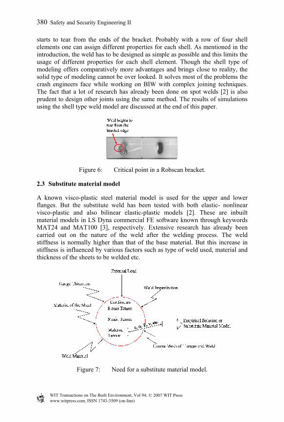
starts to tear from the ends of the bracket. Probably with a row of four shell elements one can assign different properties for each shell. As mentioned in the introduction, the weld has to be designed as simple as possible and this limits the usage of different properties for each shell element. Though the shell type of modeling offers comparatively more advantages and brings close to reality, the solid type of modeling cannot be over looked. It solves most of the problems the crash engineers face while working on BIW with complex joining techniques. The fact that a lot of research has already been done on spot welds [2] is also prudent to design other joints using the same method. The results of simulations using the shell type weld model are discussed at the end of this paper.

Figure 6: Critical point in a Robscan bracket.

2.3 Substitute material model

A known visco-plastic steel material model is used for the upper and lower flanges. But the substitute weld has been tested with both elastic- nonlinear visco-plastic and also bilinear elastic-plastic models [2]. These are inbuilt material models in LS Dyna commercial FE software known through keywords MAT24 and MAT100 [3], respectively. Extensive research has already been carried out on the nature of the weld after the welding process. The weld stiffness is normally higher than that of the base material. But this increase in stiffness is influenced by various factors such as type of weld used, material and thickness of the sheets to be welded etc.

Figure 7: Need for a substitute material model.



It is interesting to see how these effects can be taken into account while designing the material model of the weld. Because of the numerous limitations like mesh size, computational speed, weld geometry etc., all the physical properties cannot be considered in detail (fig. 7). From the set of experiments conducted, one can generalize that apart from geometry of the weld, the global force displacement curve and the failure of the substitute model depends on the two main factors viz. (i) material of the sheet and (ii) sheet thickness.

2.3.1 Effect of the sheet material on the robscan weld The yield stress and strain at failure of the weld can be related to the base material properties as follows:

BR εαε .= (4)

BoffR σσσ += (5) where Rε is the effective plastic strain in the Robscan weld, Bε the effective

plastic strain in base material, α a material parameter (0.1< α < 1.0), Rσ the

yield stress in Robscan weld, offσ the offset in the yield stress of the weld (from

hardness curves), Bσ the yield stress in base material. From physical aspect of the weld under consideration, it is evident that the steel weld material has a higher yield stress and lower strain at failure than the base material. This phenomenon is represented by offσ and α respectively. These values are purely fixed based on geometry of the weld and the substitute model. The material values for the weld are normally characterized by the material properties of the thinner gauge and also by weaker material in any gauge combination.

2.3.2 Effect of sheet thickness on the robscan weld From the set of experiments conducted on different gauge combinations, it is evident that the linear hardening modulus tE of the weld is a function of the sheet thickness used in the combination:

),( 1 δtfEt = (6)

)(δfEt = , with 2

1

tt

=δ (7)

where 21,, ttEt are the linear hardening modulus for the weld, the thickness of the first sheet, and the thickness of the second sheet, respectively. Considering the experiments conducted on the coupon level, the failure of the coupon along the weld or surrounding the weld is strongly influenced by the load angles and sheet thickness. Fig. 8 shows a KS2 0° load case of a tensile-shear specimen where normally the weld tears off due to dominant shear forces. However, Fig. 9



shows a pull out failure. This is primarily due to the thin sheet in the combination. Hence in fig. 8 one can conclude that the failure is controlled by both the sheets (refer eqn. (7)) and in fig. 9 the failure is controlled primarily by the thinner sheet (refer eqn. (6)). Experiments also reveal the relation between the focus diameter of the laser beam and the sheet thickness. If the focus diameter of the laser beam or the thickness of the weld line is close to the thickness of the thinner sheet in the combination, normally an effect shown in fig. 9 is dominant. Eqs. (4)–(7) have been summarized in fig. 10

Figure 8: “Weld tear off” due to shear loading in a 1.5mm-1.5mm gauge combination.

Figure 9: A “pull out failure” due to shear loading in a 1mm-1mm gauge combination.

Figure 10: Graphical representation of substitute material model.

The above empirical formulations have been determined keeping in mind the various effects obtained from the experiments conducted. The physical quantities like the sheet thickness cannot be directly related to material characteristics using the theory of continuum mechanics. Therefore the simplified material model is also called as the structural material model.

3 Results

Based on the above formulations for geometry and material of the Robscan weld, the results for different gauge combinations made of ZSTE340 (also known as H320LA) material for KS2 0° and KS2 90° have been shown in fig. 11.



Figure 11: Comparison of numerical and experimental force-displacement curves for different gauge combinations in a quasi static analysis.

By incorporating eqs. (4)–(7) it is possible to reproduce the experiments sufficiently. All the simulations have been carried out using MAT24, elastic- nonlinear visco-plastic material with modified stress-strain curves for the Robscan weld. Good results have also been obtained for other coupons as well.

4 Conclusions

Based on an empirical consideration of the material and sheet thickness combinations a substitute finite element model is developed for modeling Robscan laser welds in crash simulations. The crash behavior of the laser welds in the coupon crash tests is well described by the model. The substitute model will be applied to the T-components with multiple Robscan welds as further



validations to check effectiveness of the empirical formulations developed. In addition simulations are also being carried out using MAT100 [2] where the weld failure and damage of the Robscan model is possible. Development of necessary failure criteria for Robscan welds modeled by shell elements is also underway. The results obtained through this process will be tested on BIW.

References

[1] Hopf, B.: Significance of Laser Technology in Production, Production and Materials Technology, 8-11-2004

[2] Seeger, F., Fuecht, M., Frank, Th., Keding, B., Haufe, A.: An Investigation on Spot Weld Modeling for Crash Simulation with LS-DYNA, 4. LS-DYNA User Conference, Bamberg 2005

[3] LS DYNA Non Linear Analysis of Structures, User’s Manual, Livermore Software Technology Cooperation, Livermore, California 2005

[4] LS DYNA Theoretical Manual, Livermore Software Technology Cooperation, Livermore, May 1998



finite element modeling of impact strength of laser welds ... · finite element modeling of impact...

Documents