finite element modeling of electromagnetic systemsgeuzaine/elec0041/2017-02-s-course-ele… ·...
TRANSCRIPT

1
Finite Element Modeling of Electromagnetic Systems
Mathematical and numerical tools
Unit of Applied and Computational Electromagnetics (ACE) Dept. of Electrical Engineering - University of Liège - Belgium
Patrick Dular, Christophe Geuzaine
February 2015

2
Introduction
v Formulations of electromagnetic problems ♦ Maxwell equations, material relations ♦ Electrostatics, electrokinetics, magnetostatics, magnetodynamics ♦ Strong and weak formulations
❖ Discretization of electromagnetic problems ♦ Finite elements, mesh, constraints ♦ Very rich content of weak finite element formulations

3
Formulations of Electromagnetic Problems
Maxwell equations
Electrostatics
Electrokinetics
Magnetostatics
Magnetodynamics

4
Electromagnetic models ❖ Electrostatics
♦ Distribution of electric field due to static charges and/or levels of electric potential
❖ Electrokinetics ♦ Distribution of static electric current in conductors
❖ Electrodynamics ♦ Distribution of electric field and electric current in materials (insulating
and conducting)
❖ Magnetostatics ♦ Distribution of static magnetic field due to magnets and continuous
currents
❖ Magnetodynamics ♦ Distribution of magnetic field and eddy current due to moving magnets
and time variable currents
❖ Wave propagation ♦ Propagation of electromagnetic fields
All phenomena are described by Maxwell equations

5
Maxwell equations
curl h = j + ∂t d
curl e = – ∂t b
div b = 0
div d = ρv
Maxwell equations
Ampère equation
Faraday equation
Conservation equations
Principles of electromagnetism
h magnetic field (A/m) e electric field (V/m) b magnetic flux density (T) d electric flux density (C/m2) j current density (A/m2) ρv charge density (C/m3)
Physical fields and sources

6
Constants (linear relations)
Functions of the fields (nonlinear materials)
Tensors (anisotropic materials)
Material constitutive relations
b = µ h (+ bs)
d = ε e (+ ds)
j = σ e (+ js)
Constitutive relations
Magnetic relation
Dielectric relation
Ohm law
bs remnant induction, ... ds ... js source current in stranded inductor, ...
Possible sources
µ magnetic permeability (H/m) ε dielectric permittivity (F/m) σ electric conductivity (Ω–1m–1)
Characteristics of materials

7
• Formulation for • the exterior region Ω0 • the dielectric regions Ωd,j
• In each conducting region Ωc,i : v = vi → v = vi on Γc,i
e electric field (V/m) d electric flux density (C/m2) ρ electric charge density (C/m3) ε dielectric permittivity (F/m)
Electrostatics
Type of electrostatic structure
Ω0 Exterior region Ωc,i Conductors Ωd,j Dielectric
div ε grad v = – ρ
with e = – grad v
Electric scalar potential formulation
curl e = 0 div d = ρ d = ε e
Basis equations
n × e | Γ0e = 0 n ⋅ d | Γ0d = 0
& boundary conditions

8
• Formulation for • the conducting region Ωc • On each electrode Γ0e,i : v = vi → v = vi on Γ0e,i
e electric field (V/m) j electric current density (C/m2) σ electric conductivity (Ω–1m–1)
Electrokinetics
Type of electrokinetic structure
Ωc Conducting region div σ grad v = 0
with e = – grad v
Electric scalar potential formulation
curl e = 0 div j = 0 j = σ e
Basis equations
n × e | Γ0e = 0 n ⋅ j | Γ0j = 0
& boundary conditions
Γ0e,0
Γ0e,1 Γ0j
e=?, j=?
Ωc
V = v1 – v0

9 "e" side "d" side
Electrostatic problem
Basis equations curl e = 0 div d = ρ d = ε e
e = – grad v d = curl u
⊂ ⊃
ε e = d d
ρ
( u )
grad
curl
div
e
e
e
e
0
0
(– v ) F e 0
F e 1
F e 2
F e 3
div
curl
grad
d
d
d
F d 3
F d 2
F d 1
F d 0
e S 0
S e 1
S e 2
S e 3
S d 3
S d 2
S d 1
S d 0

10 "e" side "j" side
Electrokinetic problem
Basis equations curl e = 0 div j = 0 j = σ e
e = – grad v j = curl t
⊂ ⊃
σ e = j j
0
( t )
grad
curl
div
e
e
e
e
0
0
(– v ) F e 0
F e 1
F e 2
F e 3
div
curl
grad
j
j
j
F j 3
F j 2
F j 1
F j 0
e S 0
S e 1
S e 2
S e 3
S j 3
S j 2
S j 1
S j 0

11
u ≡ weak solution
u v v v v ( , L * ) - ( f , ) + Q g ( ) ds Γ ∫ = 0 , ∀ ∈ V ( Ω )
Classical and weak formulations
u ≡ classical solution
L u = f in Ω B u = g on Γ = ∂Ω
Classical formulation
Partial differential problem
Weak formulation
( u , v ) = u ( x ) v ( x ) d x Ω ∫ , u , v ∈ L 2 ( Ω )
( u , v ) = u ( x ) . v ( x ) d x Ω ∫ , u , v ∈ L 2 ( Ω )
Notations
v ≡ test function Continuous level : ∞ × ∞ system Discrete level : n × n system ⇒ numerical solution

12
Classical and weak formulations Application to the magnetostatic problem
curl e = 0 div d = 0 d = ε e
n × e ⏐Γe = 0 n . d ⏐Γd = 0 Γe Γd
Electrostatic classical formulation
Weak formulation of div d = 0
(+ boundary condition)
( d , grad v' ) = 0 , ∀ v' ∈ V(Ω)
d = ε e & e = – grad v ⇔ curl e = 0
( – ε grad v , grad v' ) = 0 , ∀ v' ∈ V(Ω) Electrostatic weak formulation with v
with V(Ω) = { v ∈ H0(Ω) ; v⏐Γe = 0 }
( div d , v' ) + < n . d , v' >Γ = 0 , ∀ v' ∈ V(Ω)
div d = 0 ⇓
n . d ⏐Γd = 0 ⇓
⇒

13
Classical and weak formulations Application to the magnetostatic problem
curl h = j div b = 0 b = µ h
n × h ⏐Γh = 0 n . b ⏐Γe = 0 Γh Γe
Magnetostatic classical formulation
Weak formulation of div b = 0
(+ boundary condition)
( b , grad φ' ) = 0 , ∀ φ' ∈ Φ(Ω)
b = µ h & h = hs – grad φ (with curl hs = j) ⇔ curl h = j
( µ (hs – grad φ) , grad φ' ) = 0 , ∀ φ' ∈ Φ(Ω) Magnetostatic weak formulation with φ
with Φ(Ω) = { φ ∈ H0(Ω) ; φ⏐Γh = 0 }
( div b , φ' ) + < n . b , φ' >Γ = 0 , ∀ φ' ∈ Φ(Ω)
div b = 0 ⇓
n . b ⏐Γe = 0 ⇓
⇒

14
Quasi-stationary approximation
Conduction current density
Displacement current density > > >
curl h = j + ∂t d
curl h = j
Electrotechnic apparatus (motors, transformers, ...) Frequencies from Hz to a few 100 kHz
Applications
Dimensions << wavelength

15
curl h = j
div b = 0
Magnetostatics
Equations
b = µ h + bs
j = js
Constitutive relations
Type of studied configuration
Ampère equation
Magnetic conservation equation
Magnetic relation
Ohm law & source current
Ω Studied domain Ωm Magnetic domain Ωs Inductor
Ω
j
Ωm
Ωs

16
curl h = j
curl e = – ∂t b
div b = 0
Magnetodynamics
Equations
b = µ h + bs
j = σ e + js
Constitutive relations
Ω p
Ω
Ω aVa
Ia
Ω sjs
Type of studied configuration
Ampère equation
Faraday equation
Magnetic conservation equation
Magnetic relation
Ohm law & source current
Ω Studied domain Ωp Passive conductor and/or magnetic domain Ωa Active conductor Ωs Inductor
17
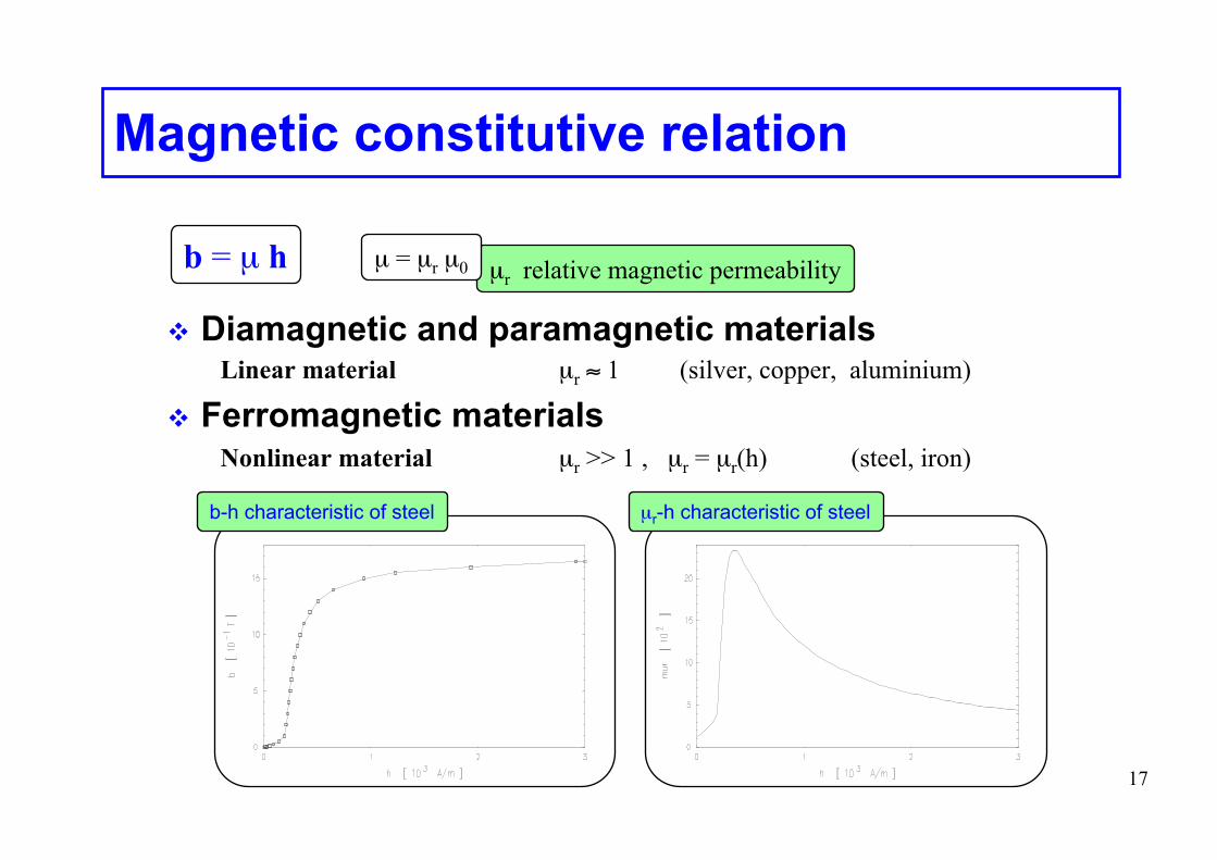
Magnetic constitutive relation
❖ Diamagnetic and paramagnetic materials Linear material µr ≈ 1 (silver, copper, aluminium)
❖ Ferromagnetic materials Nonlinear material µr >> 1 , µr = µr(h) (steel, iron)
b = µ h µr relative magnetic permeability µ = µr µ0
b-h characteristic of steel µr-h characteristic of steel

18
Maxwell equations (magnetic - static)
Magnetostatic formulations
a Formulation φ Formulation
curl h = j div b = 0
b = µ h
Ω
j
Ωm
Ωs
"h" side "b" side

19
Magnetostatic formulations
a Formulation φ Formulation
Multivalued potential Cuts
Non-unique potential Gauge condition
Magnetic scalar potential φ Magnetic vector potential a
curl ( µ–1 curl a ) = j
b = curl a
hs given such as curl hs = j (non-unique)
div ( µ ( hs – grad φ ) ) = 0
h = hs – grad φ
curl h = j div b = 0 b = µ h
Basis equations
(h) (b) (m)
⇒ (h) OK (b) OK ⇐
← (b) & (m) (h) & (m) →

20
Multivalued scalar potential
Kernel of the curl (in a domain Ω) ker ( curl ) = { v : curl v = 0 }
dom(grad)
dom(curl)
ker(curl)
cod(grad)
cod ( grad ) ⊂ ker ( curl )
cod(curl)
. 0
grad
curl
curl

21
AB AB
h . d l γ ∫ = - grad φ . d l
γ ∫ = φ A - φ B
Multivalued scalar potential - Cut
curl h = 0 in Ω h = – grad φ in Ω
Scalar potential φ ⇒ ?
OK ⇐
I
γ
Ω
(Σ)
Circulation of h along path γAB in Ω
⇒ φA – φB = 0 ≠ I ! ! !
Closed path γAB (A≡B) surrounding a conductor (with current I)
Δ φ = I
φ must be discontinuous ... through a cut

22
Vector potential - gauge condition
div b = 0 in Ω b = curl a in Ω
Vector potential a ⇒ ?
OK ⇐
b = curl a = curl ( a + grad η ) Non-uniqueness of vector potential a
Coulomb gauge div a = 0 O
P
Qex.: w(r)=r
ω vector field with non-closed lines linking any 2 points in Ω
Gauge a . ω = 0
Gauge condition

23
Magnetodynamic formulations
"h" side "b" side
Maxwell equations (quasi-stationary)
h-φ Formulation
a-v Formulation t-ω Formulation
a* Formulation
curl h = j curl e = – ∂t b
div b = 0
b = µ h j = σ e
Ω p
Ω
Ω aVa
Ia
Ω sjs

24
Magnetodynamic formulations
t-ω Formulation h-φ Formulation
Magnetic field h Magnetic scalar potential φ
Electric vector potential t Magnetic scalar potential ω
curl (σ–1 curl t) + ∂t (µ (t – grad ω)) = 0
div (µ (t – grad ω)) = 0
curl h = j curl e = – ∂t b
div b = 0 b = µ h
Basis equations
(h) (b)
curl hs = js
h ds Ωc h = hs – grad φ ds Ωc
C ⇒ (h) OK
j = σ e
curl (σ–1 curl h) + ∂t (µ h) = 0
div (µ (hs – grad φ)) = 0
j = curl t (h) OK ⇐
h = t – grad ω
← in Ωc →
← in ΩcC →
← (b) →
+ Gauge

25
Magnetodynamic formulations
a-v Formulation a* Formulation
Magnetic vector potential a* Magnetic vector potential a Electric scalar potential v
curl (µ–1 curl a) + σ (∂t a + grad v)) = js
curl h = j curl e = – ∂t b
div b = 0 b = µ h
Basis equations
(h) (b) j = σ e
curl (µ–1 curl a*) + σ ∂t a* = js
b = curl a (b) OK ⇐
e = – ∂t a – grad v
b = curl a*
⇒ (b) OK e = – ∂t a*
+ Gauge in Ω
← (h) →
+ Gauge in ΩcC

26 "h" side "b" side
Magnetostatic problem
Basis equations curl h = j div b = 0 b = µ h
hS0
Sh1
Sh2
Sh3
Se3
Se2
Se1
Se0
h = – grad φ b = curl a
⊂ ⊃
µ h = b b
0
(a)
grad
curl
div
h
h
h
h
j
0
(œφ)Fh0
Fh1
Fh2
Fh3
div
curl
grad
e
e
e
Fe3
Fe2
Fe1
Fe0

27 "h" side "b" side
Magnetodynamic problem
hS0
Sh1
Sh2
Sh3
Se3
Se2
Se1
Se0
h = t – grad φ b = curl a
⊂ ⊃
curl h = j curl e = – ∂t b
div b = 0 b = µ h
Basis equations
j = σ e
h
j
0
µ h = b b
0
e
grad
curl
div
h
h
h
j = σ e
(œφ)
(œv)
Fh0
Fh1
Fh2
Fh3
div
curl
grad
e
e
e
(t)
(a, a )*
Fe3
Fe2
Fe1
Fe0
e = – ∂t a – grad v

28
dom (grade) = Fe0 = { v ∈ L2(Ω) ; grad v ∈ L2(Ω) , v⏐Γe = 0 }
dom (curle) = Fe1 = { a ∈ L2(Ω) ; curl a ∈ L2(Ω) , n ∧ a⏐Γe = 0 }
dom (dive) = Fe2 = { b ∈ L2(Ω) ; div b ∈ L2(Ω) , n . b⏐Γe = 0 }
Boundary conditions on Γe
dom (gradh) = Fh0 = { φ ∈ L2(Ω) ; grad φ ∈ L2(Ω) , φ⏐Γh = 0 }
dom (curlh) = Fh1 = { h ∈ L2(Ω) ; curl h ∈ L2(Ω) , n ∧ h⏐Γh = 0 }
dom (divh) = Fh2 = { j ∈ L2(Ω) ; div j ∈ L2(Ω) , n . j⏐Γh = 0 }
Boundary conditions on Γh
Function spaces Fe0 ⊂ L2, Fe
1 ⊂ L2, Fe2 ⊂ L2, Fe
3 ⊂ L2
Function spaces Fh0 ⊂ L2, Fh
1 ⊂ L2, Fh2 ⊂ L2, Fh
3 ⊂ L2 Basis structure
Basis structure
Continuous mathematical structure
gradh Fh0 ⊂ Fh
1 , curlh Fh1 ⊂ Fh
2 , divh Fh2 ⊂ Fh
3
F h 0 grad h ⎯ → ⎯ ⎯ ⎯ F h
1 curl h ⎯ → ⎯ ⎯ F h 2 div h ⎯ → ⎯ ⎯ F h
3 Sequence
gradh Fe0 ⊂ Fe
1 , curle Fe1 ⊂ Fe
2 , dive Fe2 ⊂ Fe
3
F e 3 div e ← ⎯ ⎯ ⎯ F e
2 curl e ← ⎯ ⎯ ⎯ F e 1 grad e ← ⎯ ⎯ ⎯ ⎯ F e
0 Sequence
Domain Ω, Boundary ∂Ω = Γh U Γe

29
Discretization of Electromagnetic Problems
Nodal, edge, face and volume finite elements

30
Discrete mathematical structure
Continuous function spaces & domain Classical and weak formulations
Continuous problem
Finite element method
Discrete function spaces piecewise defined in a discrete domain (mesh)
Discrete problem
Discretization Approximation
Classical & weak formulations → ? Properties of the fields → ?
Questions To build a discrete structure
as similar as possible as the continuous structure
Objective

31
Discrete mathematical structure
Sequence of finite element spaces Sequence of function spaces & Mesh
Finite element space Function space & Mesh
!
!+ f i
i ∪!
+ f i i ∪!
⎧ ⎨ ⎩ ⎪
⎫ ⎬ ⎭ ⎪
Finite element Interpolation in a geometric element of simple shape
+ f

32
Finite elements
❖ Finite element (K, PK, ΣK) ♦ K = domain of space (tetrahedron, hexahedron, prism) ♦ PK = function space of finite dimension nK, defined in K ♦ ΣK = set of nK degrees of freedom
represented by nK linear functionals φi, 1 ≤ i ≤ nK, defined in PK and whose values belong to IR
IR
cod(f)K = dom(f) f ∈ P
xf(x)
φ (f)i
κ
K

33
Finite elements
❖ Unisolvance ∀ u ∈ PK , u is uniquely defined by the degrees of freedom
❖ Interpolation ❖ Finite element space
Union of finite elements (Kj, PKj, ΣKj) such as : ❍ the union of the Kj fill the studied domain (≡ mesh) ❍ some continuity conditions are satisfied across the element
interfaces
Basis functions
Degrees of freedom
u K = φ i ( u ) p i i = 1
n K
∑

34
Sequence of finite element spaces
Geometric elements Tetrahedral
(4 nodes) Hexahedra
(8 nodes) Prisms (6 nodes)
Mesh
Geometric entities
Nodes i ∈ N
Edges i ∈ E
Faces i ∈ F
Volumes i ∈ V
Sequence of function spaces S0 S1 S2 S3

35
Sequence of finite element spaces
{si , i ∈ N}
{si , i ∈ E}
{si , i ∈ F}
{si , i ∈ V}
Bases Finite elements
S0
S1
S2
S3 Volume element
Point evaluation
Curve integral Surface integral Volume integral
Nodal value
Circulation along edge Flux across
face Volume integral
Functions Functionals Degrees of freedom Properties
si (x j) = δij∀ i, j ∈N
si . n dsj∫ = δij
∀ i, j ∈F
si dvj∫ = δij
∀ i, j ∈V
uK = φi (u) sii∑
Face element
Edge element
Nodal element
si . dlj∫ = δij
∀ i , j ∈ E

36
Sequence of finite element spaces
Base functions
Continuity across element interfaces
Codomains of the operators
{si , i ∈ N} value
{si , i ∈ E} tangential component grad S0 ⊂ S1
{si , i ∈ F} normal component curl S1 ⊂ S2
{si , i ∈ V} discontinuity div S2 ⊂ S3
Conformity S 0 grad
⎯ → ⎯ ⎯ S 1 curl ⎯ → ⎯ ⎯ S 2 div
⎯ → ⎯ ⎯ S 3
Sequence
S0
S1 grad S0
S2 curl S1
S3 div S2
S0
S1
S2
S3

37
Function spaces S0 et S3
For each node i ∈ N → scalar field
0
0 0
0 0
0 0
0
0
0 pi = 1 node i
si (x) = pi (x) ∈ S0
p i = 1 at node i 0 at all other nodes
⎧ ⎨ ⎩
p i continuous in Ω
sv = 1 / vol (v) ∈ S3
For each Volume v ∈ V → scalar field

38
Edge function space S1
For each edge eij = {i, j} ∈ E → vector field
se ∈ S1
m
p
o
n n
m
qp
o
NF,mn = {i∈N ; i∈fmop(q ) , o, p,q ≠ n}
N.B.: In an element : 3 edges/node
Illustration of the vector field se Definition of the set of nodes NF,mn -
s e ij = p j grad p r r ∈ N F , j i
∑ - p i grad p r r ∈ N F , i j
∑
e ij
s ei
j
NF, ij-NF, ji
-
39
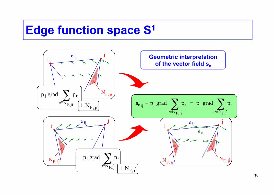
Edge function space S1
e ijij
NF, ij-
e ijij
NF, ji-
Geometric interpretation of the vector field se
p j grad p r r ∈ N F j , i
∑ ⊥ N F , j i
s e ij = p j grad p r r ∈ N F , j i
∑ - p i grad p r r ∈ N F , i j
∑
- p i grad p r r ∈ N F , i j
∑ ⊥ N F , i j
e ij
s ei
j
NF, ij-NF, ji
-

40
Function space S2
i
j
k
NF, ij-
NF, ji-
NF, jk-
NF, ki-
NF, ik-
NF, kj-
f ijk
For each facet f ∈ F → vector field f = fijk(l) = {i, j, k (, l) } = {q1, q2, q3 (, q4) }
Illustration of the vector field sf
s f = a f p q c c = 1
# N f
∑ grad p r r ∈ N F , q c q c + 1 ∑ ⎛
⎝ ⎜
⎞
⎠ ⎟ ∧ grad p r r ∈ N F , q c q c - 1
∑ ⎛
⎝ ⎜
⎞
⎠ ⎟
sf ∈ S2
3 → af = 2 #Nf =
4 → af = 1

41
Particular subspaces of S1
Ampere equation in a domain Ωc
C without current
(↔ Ωc)
Applications
Gauge condition on a vector potential
Definition of a generalized source field hs
such that curl hs = js
h ∈ S1(Ω) ; curl h = 0 in ΩcC ⊂ Ω → h ≡ ?
a ∈ S1(Ω) ; b = curl a ∈ S2(Ω) → a ≡ ? Gauge a . ω = 0 to fix a
Kernel of the curl operator
Gauged subspace

42
Kernel of the curl operator
Ω c ∂ Ω c
E c
h k
φ n
φ n'
Ω c C
N c , E c C C N c , E c C C
(interface)
Base of H ≡ basis functions of • inner edges of Ωc • nodes of Ωc
C, with those of ∂Ωc
H = { h ∈ S 1 ( Ω ) ; curl h = 0 in Ω c C }
with
h = h k s k k ∈ E c
∑ + φ n v n n ∈ N c
C ∑
v n = s nj nj ∈ E c
C ∑
h l l ∈ E c
C h = h a s a
e ∈ E ∑ = h k s k
k ∈ E c
∑ + s l ∑
h l = h . dl l ab
∫ = - grad φ . dl l ab
∫ = φ a l - φ b l
( h = h k s k k ∈ E c
∑ + ) s l l ∈ E c
C ∑ a l - φ b l φ
h = – grad φ in ΩcC
Case of simply connected domains

43
Kernel of the curl operator
H = { h ∈ S 1 ( Ω ) ; curl h = 0 in Ω c C }
φ+ – φ– = φ⏐Γ+eci – φ⏐Γ–
eci = Ii
qi • defined in ΩcC
• unit discontinuity across Γeci • continuous in a transition layer • zero out of this layer
φ = φcont + φdisc
discontinuity of φdisc
with
edges of ΩcC
starting from a node of the cut and located on side '+'
but not on the cut
h = h k s k k ∈ A c
∑ + φ cont n v n
n ∈ N c C
∑ + I i c i i ∈ C ∑
c i = s nj nj ∈ A c
C
n ∈ N ec i j ∈ N c
C +
j ∉ N ec i
∑
φ disc = I i q i i ∈ C ∑
Basis of H ≡ basis functions of • inner edges of Ωc • nodes of Ωc
C • cuts of C
(cuts) h = – grad φ in Ωc
C
Case of multiply connected domains

44
Gauged subspace of S1
b = curl a
co-tree !⌣ !E
Tree ≡ set of edges connecting (in Ω) all the nodes of Ω without
forming any loop (E) Co-tree ≡ complementary set of the tree (E)
⌢ !⌣ !
a = a e s e e ∈ E ∑ ∈ S 1 ( Ω ) , b = b f s f
f ∈ F ∑ ∈ S 2 ( Ω )
!a = a i s i
i ∈ ⌣ !E ∑ ∈
⌣ !S 1 ( Ω )
S1(Ω) = {a ∈ S1(Ω) ; aj = 0 , ∀ j ∈ E} ⌣ !⌣ !
Gauged space of S1(Ω)
with
b f = i ( e , f ) a e e ∈ E ∑ , f ∈ F matrix form: bf CFE
ae =
Face-edge incidence matrix
Gauged space in Ω
tree !⌢ !E
Basis of S1(Ω) ≡ co-tree edge basis functions (explicit gauge definition)
⌣ !

45
❖ Electromagnetic fields extend to infinity (unbounded domain)
♦ Approximate boundary conditions:
❍ zero fields at finite distance
♦ Rigorous boundary conditions:
❍ "infinite" finite elements (geometrical transformations)
❍ boundary elements (FEM-BEM coupling)
❖ Electromagnetic fields are confined (bounded domain) ♦ Rigorous boundary conditions
Mesh of electromagnetic devices

46
❖ Electromagnetic fields enter the materials up to a distance depending of physical characteristics and constraints
♦ Skin depth δ (δ<< if ω, σ, µ >>)
♦ mesh fine enough near surfaces (material boundaries)
♦ use of surface elements when δ → 0
δω σ µ
=2
Mesh of electromagnetic devices

47
❖ Types of elements
♦ 2D : triangles, quadrangles
♦ 3D : tetrahedra, hexahedra, prisms, pyramids
♦ Coupling of volume and surface elements
❍ boundary conditions
❍ thin plates
❍ interfaces between regions
❍ cuts (for making domains simply connected)
♦ Special elements (air gaps between moving pieces, ...)
Mesh of electromagnetic devices

48
Constraints in partial differential problems
❖ Local constraints (on local fields) ♦ Boundary conditions
❍ i.e., conditions on local fields on the boundary of the studied domain ♦ Interface conditions
❍ e.g., coupling of fields between sub-domains
❖ Global constraints (functional on fields) ♦ Flux or circulations of fields to be fixed
❍ e.g., current, voltage, m.m.f., charge, etc. ♦ Flux or circulations of fields to be connected
❍ e.g., circuit coupling Weak formulations for finite element models
Essential and natural constraints, i.e., strongly and weakly satisfied

49
Constraints in electromagnetic systems
❖ Coupling of scalar potentials with vector fields ♦ e.g., in h-φ and a-v formulations
❖ Gauge condition on vector potentials ♦ e.g., magnetic vector potential a, source magnetic field hs
❖ Coupling between source and reaction fields ♦ e.g., source magnetic field hs in the h-φ formulation,
source electric scalar potential vs in the a-v formulation
❖ Coupling of local and global quantities ♦ e.g., currents and voltages in h-φ and a-v formulations
(massive, stranded and foil inductors)
❖ Interface conditions on thin regions ♦ i.e., discontinuities of either tangential or normal components
Interest for a “correct” discrete form of these constraints
Sequence of finite element
spaces

50
Complementary 3D formulations
∂ µ σt scurl curle
( , ' ) ( , ' ) , 'h h h h n e hΩ Ω Γ+ + < × > =−1 0 ∀ ∈h' ( )Fh1 Ω
( , ' ) ( , ' ) , 'µ σ ∂− + + < × > =1 0curl curl t s ha a a a n h aΩ Ω Γ ∀ ∈a' ( )Fe1 Ω
Magnetodynamic h-formulation
Magnetodynamic a-formulation
How to enforce global fluxes ?

51
h-φ formulation
❖ h-φ magnetodynamic finite element formulations with massive and stranded inductors
❖ Use of edge and nodal finite elements for h and φ ♦ Natural coupling between h and φ ♦ Definition of current in a strong sense with basis functions either for massive
or stranded inductors ♦ Definition of voltage in a weak sense ♦ Natural coupling between fields, currents and voltages ♦ etc.

52
a-v formulation
❖ a-vs Magnetodynamic finite element formulation with massive and stranded inductors
❖ Use of edge and nodal finite elements for a and vs ♦ Definition of a source electric scalar potential vs in massive inductors in an
efficient way (limited support) ♦ Natural coupling between a and vs for massive inductors ♦ Adaptation for stranded inductors: several methods ♦ Natural coupling between local and global quantities, i.e. fields and currents
and voltages ♦ etc.

53
Strong and weak formulations
curl h = js
div b = ρs
b = µ h
Constitutive relation
Equations
Boundary conditions (BCs)
,h bs sΓ Γ× = × ⋅ = ⋅n h n h n b n b
in Ω
h = hs - grad φ , with curl hs = js
b = bs + curl a , with div bs = ρs
Scalar potential φ
Vector potential a
gradb b
uΓ Γ× = ×n a n
heach non-connected portion of constantΓφ =
Strongly satisfies

54
Strong formulations
curl e = 0 , div j = 0 , j = σ e , e = - grad v or j = curl u
Electrokinetics
curl e = 0 , div d = ρs , d = ε e , e = - grad v or d = ds + curl u
Electrostatics
curl h = js , div b = 0 , b = µ h , h = hs - grad φ or b = curl a
Magnetostatics
curl h = j , curl e = – ∂t b , div b = 0 , b = µ h , j = σ e + js , ...
Magnetodynamics

55
Grad-div weak formulation 1 1grad div div( ) , ( ), ( )v v v v H⋅ + = ∈ Ω ∈ Ωu u u u H
, , ',(( ,g 'rad , 0') , '')bs bss R
ρ φΓΩ Ω Γ φ+ < ⋅ φ + < ⋅ φ >− −φ => =ρ φ n b n bb
(div , ') , 'bs sΩ Γ= φ < φ− − >⋅ρ ⋅− n n bbb
, 'Electrokinetics: ( ,grad ') , ' , ' (div , ') , 'j v js s j vv v v v v RΩ Γ Γ Ω Γ− + < ⋅ > + < ⋅ > = − < ⋅ − ⋅ > =j n j n j j n j n j
, 'Electrostatics: ( ,grad ') ( , ') , ' , ' (div , ') , 's d v ds s d vv v v v v v RΩ Ω Γ Γ Ω Γ− − ρ + < ⋅ > + < ⋅ > = −ρ − < ⋅ − ⋅ > =d n d n d d n d n d
( ,grad ) (div , ) ,v v vΩ ∂ΩΩ+ = < ⋅ >u u n u
grad-div Green formula
,add on both sides: ( , ') , '
s bss ρΩ Γ− ρ φ + < ⋅ φ >n b
integration in Ω and divergence theorem
grad-div scalar potential φ weak formulation
( grad )s=µ − φb h
sMagnetostatics: 0ρ =

56
Curl-curl weak formulation
curl-curl Green formula
,add on both sides ( , '): , '
hs js sΩ Γ− + < × >j n h aa
integration in Ω and divergence theorem
curl-curl vector potential a weak formulation
( ,curl ) (cu l , ) ,r ∂ΩΩ Ω − >= < ×−u v u n u vv
1curl curl div( ) , , ( )⋅ − ⋅ = × ∈ Ωu v v u v u u v H
(curl , ') , 'hss Ω Γ−= − × >−< ×n ha aj n hh
, , ',(( , 0',curl ') ,') 's j bh as hs RΓΩ ΓΩ + < × >− + < × = =>n h n h aaj ah a
1( curl )s−=µ +h b a

57
Grad-div weak formulation
1
, ',( ,grad ) ( , )' ' ', 0s b pp p ps s bRρΩ Ω Γ φ− − ρ +φ φ < ⋅ >φ = ≠n bb
,( ,grad ') ' '( , ) , 0
s bp p p s ps ρΩ Ω Γ− + − ρ + < ⋅ >φ φ =φ bb nb
Use of hierarchal TF φp' in the weak formulation
Error indicator: lack of fulfillment of WF
... can be used as a source for a local FE problem (naturally limited to the FE support of each TF) to calculate the higher order correction bp to be given to the actual solution b for satisfying the WF... solution of :
, ''( ,grad )pp p bRΩ φ= −φbor Local FE problems 1

58
A posteriori error estimation (1/2) V
Hig
her o
rder
hie
rarc
hal c
orre
ctio
n v p
(2
nd o
rder
, BFs
and
TFs
on
edge
s)
Elec
tric
sca
lar
pot
entia
l v
(1st
ord
er)
Large local correction ⇒ Large error
Coarse mesh Fine mesh
Electric field
Field discontinuity directly
Electrokinetic / electrostatic problem

59
Curl-curl weak formulation
2
, , '( ,curl ) ( , ) ,' 0' 's j h pp p ps h as RΩ Ω Γ ≠− + < × > =j n hah a a
, ''( ,curl )pp p ahRΩ = −h a
Use of hierarchal TF ap' in the weak formulation
Error indicator: lack of fulfillment of WF
... also used as a source to calculate the higher order correction hp of h... solution of :
Local FE problems 2

60
A posteriori error estimation (2/2) Magnetostatic problem Magnetodynamic problem
Mag
netic
vec
tor
pot
entia
l a
(1st
ord
er)
Hig
her o
rder
hie
rarc
hal
corr
ectio
n a p
(2nd
ord
er,
BFs
and
TFs
on
face
s)
Coarse mesh
Fine mesh
skin depth
Large local correction ⇒ Large error
Conductive core Magnetic core
V