finite element modeling for ultrasonic transducersthis is a preprint of a paper published in proc....
TRANSCRIPT

(This is a preprint of a paper published in Proc. SPIE Int. Symp. Medical Imaging 1998, San Diego, Feb 21-27, 1998Ultrasonic Transducer Engineering Conference, edited by K. Shung)
Finite Element Modeling for Ultrasonic Transducers
Najib N. Abbouda, Gregory L. Wojcikb, David K. Vaughanb,John Mouldb, David J. Powellb, Lisa Nikodymb
aWeidlinger Associates Inc., 375 Hudson Street, New York, NY 10014, USAbWeidlinger Associates Inc., 4410 El Camino Real, Los Altos, CA 94022, USA
ABSTRACTFinite element modeling is being adopted in the design of ultrasonic transducers and imaging arrays.Impetus is accelerated product design cycles and the need to push the technology. Existing designs arebeing optimized and new concepts are being explored. This recent acceptance follows the convergence ofimprovements on many fronts: necessary computer resources are more accessible, lean, specializedalgorithms replacing general-purpose approaches, and better material characterization
The basics of the finite element method (FEM) for the coupled piezoelectric-acoustic problem arereviewed. We contrast different FEM formulations and discuss the implications of each: time-domainversus frequency domain, implicit versus explicit algorithms, linear versus nonlinear. Beyond discussionsof the theoretical underpinnings of numerical methods, the paper also examines other modeling ingredientssuch as discretization, material attenuation, boundary conditions, farfield extrapolation, and electriccircuits.
Particular emphasis is placed on material characterization, and this is discussed through an actual "model-build-test" validation sequence, undertaken recently. Some applications are also discussed.
Keywords: Arrays, Attenuation, Finite Element Method, Imaging, Piezoelectric, Transducer, Ultrasound
1. INTRODUCTIONUntil recently, medical transducer designers relied almost exclusively on 1D analytical models andexperimental prototypes. Now, many employ comprehensive finite element simulations for transient, 2Dand 3D analyses. Effectiveness of their modeling is proportional to accuracy and completeness of materialmeasurements, fidelity of geometrical and manufacturing process details, and the modeler's skill withnumerical experiments and design strategies. Modeling skills rely on an intuitive understanding of thetransducer's operational parameters and the overall design problem. This requires either years ofexperience or focused, practical training. Without such skills, modeling is often used poorly and resultsmay be misinterpreted or erroneous, leading to wasted resources and market opportunities. As personalcomputers, modern finite element algorithms, and user interfaces make 2D/3D modeling more accessible,the required skill set needs to be taught quickly and efficiently to an eclectic mix of users.
Therefore, in our role as code developers, users, and trainers, we have sought a simple yet practical basisfor teaching transducer fundamentals and the finite element modeling paradigm. The most direct basiswould be closed-form solutions, but transducers generally have too many characteristic lengths for simplemathematical analysis. However, note that each segment of a typical medical transducer has a fairly shortextensional resonance length, e.g., | O/2 for the piezoceramic and | O/4 for the matching layer(s). Thesefractional-wave dimensions suggest that relatively low frequency coupled oscillators rather thanpropagating waves can provide a simple, intuitive model of device physics. Although oscillator modelscannot be quantitative, in general, they provide the simplest, complete representation of 1Delectromechanical transducer behavior. This approach appears to have been passed over in the transducerliterature and as a teaching aid. To this end, Section 2 examines simple spring-mass models thatdemonstrate basic device behavior and as well as introduce finite element fundamentals, given that springsand masses are the simplest "elements" of discrete numerical modeling.
a correspondence: Email: [email protected], Tel: (212) 367-3000, Web: www.wai.comb correspondence: Email: [email protected], Tel: (650) 949-3010, Web: www.wai.com

2
We then proceed in Section 3 to generalization of these electromechanical models, leading to the full 3Dfinite element formalism. This was first developed by Allik and Hughes in 1970 [1]. Although in use sincethen for analysis of low-frequency underwater projectors [2], its adoption in the medical ultrasoundcommunity remained limited until the early 1990's. The investigation of the then new 1-3 piezocompositesaccentuated the need for such comprehensive modeling, as exemplified by the work of Hossack andHayward [3]. The work of Lerch [4] emphasized the need for transient response modeling and non-uniformdamping in realistic applications, features lacking in then available commercial software. It is the adoptionof explicit wave propagation algorithms in PZFlex [5-11] however that made realistic transducersimulations practical. With demonstrated speed/size advantage factors of 100 over conventional implicitalgorithms, broadband imaging transducer models became tractable on desktop computers. The point is thatsoftware used in a production capacity must rely on specialized algorithms rather than general-purposeones. To this end, we contrast different FEM formulations and discuss the implications of each: time-domain versus frequency domain, implicit versus explicit algorithms, and linear versus nonlinear schemes.
Beyond discussions of the theoretical underpinnings of numerical methods, we examine in Section 4modeling issues from the analyst's perspective: discretization, material dissipation, boundary conditions,farfield extrapolation, and electric circuits. The "quality" and "cost effectiveness" of the model depends onthe proper use of these ingredients. We review their underlying assumptions and provide guidelines foroptimal use.
Accuracy of the finite element model also hinges on accuracy of the material constitutive properties, andthose provided in manufacturer specification sheets are often incomplete, if not inaccurate. Section 5examines material characterization issues in the context of a recently undertaken validation exercise basedon an incremental "model-build-test" analysis of a nonproprietary 1D biomedical imaging array. Thissequence of component and device validations provides an excellent opportunity to identifycharacterization procedures that work and those that require further refinement, all while displaying itsimpact on the resultant finite element solution. Ultimately, validated and established characterizationprotocols are critical if numerical modeling is to serve as a "virtual prototyping" tool.
Some recent applications and studies are briefly discussed in Section 6, mainly to highlight some of theimportant points made earlier, to mention new ones that could not be discussed in detail in the body of thepaper, and to provide some references to a broader range of applications.
2. COUPLED OSCILLATOR MODELS OF RESONANT TRANSDUCERSEach segment of a typical medical transducer has a fairly short extensional resonance length, e.g., | O/2 forthe piezoceramic and | O/4 for the matching layer(s). These fractional-wave dimensions suggest thatrelatively low frequency coupled oscillators rather than propagating waves can provide a simple, intuitivemodel of device physics. Although oscillator models cannot be quantitative, in general, they provide thesimplest, complete representation of 1D electromechanical transducer behavior. As such, they are valuablein illustrating the "fundamentals".
To this end we examine what amounts to spring-mass models of transducer stack elements. These are themost fundamental electromechanical analogs and can be developed intuitively, as follows, or from morerigorous matrix structural analysis and finite element concepts. In particular, piezoelectric constitutiverelations for the spring are derived from the continuum relations and applied to the simple harmonicoscillator. This is generalized to a coupled oscillator representing the lowest-order resonances in apiezoelectric transducer stack, i.e., backing, piezoelectric, matching layer(s), and water load.
2.1. Equations of motion and constitutive relationsThe basis for approximate dynamic models, in general, is (1) assumption of a specific strain function, e.g.,constant or linear, and (2) mass distribution, i.e., consistent or lumped. This is the foundation of matrixstructural analysis [12], the predecessor of finite element methods. The strain function assumption yieldsordinary differential equations in time by reducing the infinite degrees of freedom to a finite number, whilethe mass distribution assumption simplifies time integration.

3
Consider a 1D piezoelectric bar with length L and area A, electroded on the ends and poled lengthwise.Longitudinal displacement is u(x,t), governed by the partial differential equation
x
T
t
uA
w
w
w
wU
2
2
(2.1)
where x is the space coordinate, t is time, U is material density, and T(x,t) is longitudinal stress. Boundaryconditions are specified on u or T, along with initial conditions. The piezoelectric constitutive relationsbetween stress T, strain S = wu/wx, electric field E, and electric displacement D are
eSEDeEScT SE� � H, (2.2)
where Ec is elastic stiffness under constant electric field, e is the piezoelectric stress constant, and SH iselectric permittivity under constant strain, e.g., see [13]. Because 0 �� D (divergence condition onelectric displacement) and the absence of free charge, D(t) is uniform over the bar.
The simplest approximation of the bar's dynamics follows from the constant strain assumption and masslumping. This is equivalent to a linear spring separating equal end masses m = UAL/2, as shown in Fig. 1.End displacements u1 and u2 are the degrees of freedom, whence governing equation (2.1) simplifies to theordinary differential equations
222
2
121
2
, FFdt
udmFF
dt
udm sprspr �� � (2.3)
where Fspr is the spring force and F1, F2 are external forces applied at each end. Multiplying (2.2) by Aand defining spring force Fspr{-AT, electrode charge Q { AD, spring compression u { u1 – u2 { LS, and
voltage V { LE yields the piezoelectric spring constitutive relations
ueVCQVeudukF Sm
Espr ˆ,ˆ � ��� � (2.4)
LACLAeeLAck SSEE /,/ˆ,/ H{{{ (2.5)
where kE, ˆ e , and CS are spring stiffness, piezoelectric force constant, and capacitance, respectively. Notethat the spring equation is generalized above to include rate dependent mechanical damping through dm.The sign convention on u is positive for compression and negative for extension. The spring idealization,governing equations, and constitutive relations are illustrated in Figure 1.
��
��
V V
T = cES - eE , D = εSE + eS
L
F = -kE(u1-u2) + êV , Q = CSV + ê(u1-u2)
A
u1 u2
m m
x
T
t
uA
ww
w
w2
2
U 222
2
121
2
, FFdt
udmFF
dt
udm sprspr � �
Fig. 1. Longitudinal piezoelectric oscillator (left) of length L and area A, and theequivalent simple harmonic oscillator model (right), showing the correspondingpiezoelectric constitutive relations (above) and governing equations (below).
2.2. Simple harmonic oscillator solutionsCombining the spring-mass equations of motion and the spring constitutive relations yields two ordinarydifferential equations governing the piezoelectric oscillator. For example, consider the symmetric problem,i.e., F1 = -F2 = Fext and u1 = -u2, whence (2.3) and (2.4) yield
1111 ˆ2,ˆ22 ueVCQFVeukudum Sext
Em � � �� ��� (2.6)
Two canonical cases of interest are the "send" problem defined by voltage input and displacement output,and the "receive" problem defined by external force input and voltage output.

4
For the send problem, the differential equation and constitutive relation for current i = d Q� /dt are
1111 ˆ2,ˆ22 ueVCiVeukudum SEm �
�
��� � �� (2.7)
When the prescribed voltage is time harmonic, tjeVtV Z
0)( , steady solutions are tjeutu Z
01 )( and
substituting gives
Em kdjm
e
V
u
22
ˆ2
0
0
���
ZZ(2.8)
Electromechanical response is given by the electrical impedance, i.e., voltage divided by current,
¸̧¹
·¨̈©
§
��
��
�� 0for
ˆ2)2(
2ˆ2
122
2
00mES
E
Sd
emkC
mkj
VueC
j
i
V
Z
Z
ZZ(2.9)
For the receive problem assume that current vanishes, hence, Q = Q0 = 0 (without loss of generality, sinceQ0 produces static compression and voltage that are removable by redefining equilibrium position andground potential). The governing equation and constitutive relation for voltage become
0ˆ,22 1111 � �� ueVCFukudum Sext
Dm ���
(2.10)
where kD is the stiffened spring constant
SESEED
c
e
Ck
eKKkk
H
2222 ˆ
,)1( {�{ (2.11)
and K is the piezoelectric coupling constant. For time harmonic external force, tjext eFtF Z
0)( , steady
solutions are tjeutu Z
01 )( , tjeVtV Z
0)( and substituting gives
¸¹
ᬩ
§ �
��
0for2
1
22
122
0
0mD
mD
dmkdjmkF
u
ZZZ(2.14)
Output sensitivity is defined as voltage divided by force,
¸̧¹
·¨̈©
§
�
� � 0for
)2(
ˆ2ˆ22
0
0mDSS
ext
dmkC
e
F
u
C
e
F
V
Z(2.15)
These simple, closed-form solutions exhibit most of the piezoelectric resonator characteristics that are ofinterest to the designer and modeler. Of course they are crude approximations despite being completerepresentations of 1D transducer physics. In contrast, more comprehensive models of the type described inthis paper provide more complete, quantitative answers but without simple functional relations.
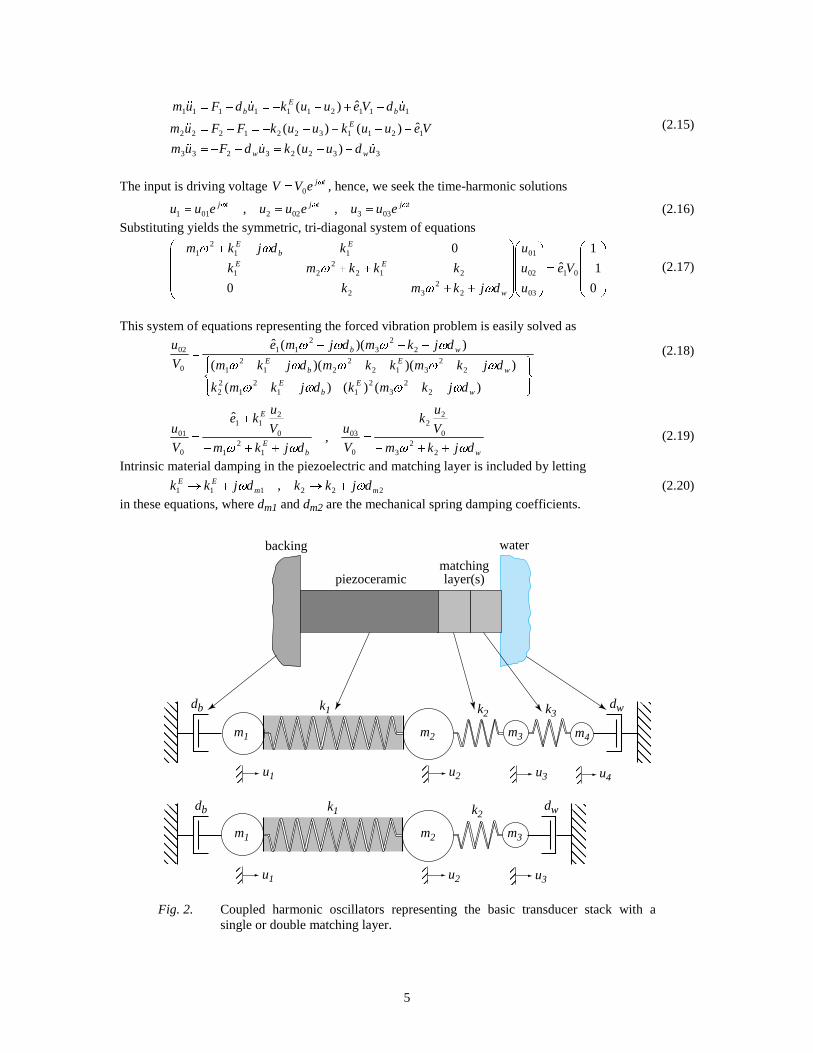
2.3. Coupled harmonic oscillator solutionsGeneralizing the single piezoelectric oscillator described above to a coupled oscillator representing atransducer stack is straightforward and illustrated in Figure 2. The piezoelectric ceramic and matchinglayer(s) are replaced by piezoelectric or elastic springs with half of the mass lumped at each end. Thewater and backing loads are represented by dashpots with coefficient d = ImA where Im is mechanicalimpedance of the load medium and A is cross-sectional area of the stack. This follows from 1D wavetheory, which states that pressure p and velocity x� are related as p = -Imx� where Im { Uc is themechanical impedance of the medium.
Consider the single matching layer case. Coefficients and spring forces are
)(,ˆ)(
,
,,
3222112111
21
22221
331211121
1
uukFVeuukF
AvdAvd
ALmmmmALm
E
LwwwLbbb
�� ���
�
UU
UU
(2.14)
where vLb and vLw are wave speeds (longitudinal) in the backing and water load. For simplicity we ignoreintrinsic damping in the matching layer and piezoceramic. Equations of motion for the three masses are
5
33223233
12113221222
1112111111
)(
ˆ)()(
ˆ)(
uduukudFum
VeuukuukFFum
udVeuukudFum
ww
E
bE
b
����
��
����
�� ��
����� �
���� � (2.15)
The input is driving voltage tjeVV Z
0 , hence, we seek the time-harmonic solutionstjtjtj euueuueuu ZZZ
033022011 ,, (2.16)
Substituting yields the symmetric, tri-diagonal system of equations
¸¸¸
¹
·
¨¨¨
©
§�
¸¸¸
¹
·
¨¨¨
©
§
¸¸¸
¹
·
¨¨¨
©
§
����
�����
����
0
1
1
ˆ
0
0
01
03
02
01
22
32
2122
21
112
1
Ve
u
u
u
djkmk
kkkmk
kdjkm
w
EE
Eb
E
ZZ
Z
ZZ
(2.17)
This system of equations representing the forced vibration problem is easily solved as
°¿
°¾½
°̄
°®
�����
�������
���
)()()(
))()((
))((ˆ
22
32
112
122
22
3122
212
1
22
32
11
0
02
wE
bE
wE
bE
wb
djkmkdjkmk
djkmkkmdjkm
djkmdjme
V
u
ZZZZ
ZZZZZ
ZZZZ (2.18)
wbE
E
djkm
V
uk
V
u
djkm
V
uke
V
u
ZZZZ ���
�
���
�
2
23
0
22
0
03
12
1
0
211
0
01 ,
ˆ
(2.19)
Intrinsic material damping in the piezoelectric and matching layer is included by letting
222111 , mmEE djkkdjkk ZZ �o�o (2.20)
in these equations, where dm1 and dm2 are the mechanical spring damping coefficients.
�������
�����
���
m1 m2 m3 m4
u1 u2
k1 dwdb k2 k3
����
u3 u4
�����
������
water
matchinglayer(s)piezoceramic
backing
�������
�����
���
m1 m2 m3
u1 u2
k1 dwdb k2
����
u3�������
Fig. 2. Coupled harmonic oscillators representing the basic transducer stack with asingle or double matching layer.
6
On this basis, closed-form solutions of coupled piezoelectric oscillator models are easily studied. They arethe manifest, low order limit of representations ranging from electrical analogs like Mason and KLMmodels, to 1D wave propagation models, to broadband (transient) 2D and 3D finite element models. Interms of utility, such models have proven convenient as a "trivial" mathematical basis for demonstratinggeneric device behavior, and more specifically, for teaching fundamentals, illustrating matching layerdesign issues, and qualitative interpretations of transducer experiments and numerical simulations. More tothe point, they are the archetype for 2D/3D finite element transducer models and an intuitive guide toproper electromechanical device modeling, particularly if the engineer's background has focused onelectrical analog interpretations.
3. ALGORITHMIC FORMULATION OF PIEZOELECTRIC FINITE ELEMENTSThe concepts illustrated by the simple oscillator models above are generalized to full 3D behavior next,leading to the complete finite element formulation. This entails a dimensionality extension of course, butmainly raises the issue of effective computer-based solution schemes.
3.1. Governing differential equations (strong form)Conventional polarized ferroelectric ceramics used in the manufacture of ultrasonic transducers aregoverned by the constitutive relations for linear piezoelectricity [13] and by the equations of mechanicaland electrical balance. The electric balance is assumed instantaneous and decoupled, i.e., the quasi-staticapproximation of the electric field relative to the mechanical field. The governing equations are thusexpressed:
ESeDEeSCT ��� ��� sTEHH, - constitutive equations- (3.1)
Tu �� ��U - momentum balance - (3.2)
0 �� D - electric balance - (3.3)
with I�� �� EuS ,s
where T, S, E, D are the mechanical stress, mechanical strain, electric field and electric displacementvectors, respectively. CE, HHs, e are the matrices of stiffness constants at constant electric field, of dielectricconstants at constant strain, and of piezoelectric coupling constants, respectively. u is the mechanical
displacement vector and 22 tww uu�� is the acceleration, each superposed dot "." denoting one time
differentiation. I is the electric potential (voltage). To complete the description of the problem, equations(3.1)-(3.3) are complemented by appropriate boundary conditions, such as prescribed displacements orvoltages, and applied forces or electric charge. These equations are the 3D counterparts to (2.1) and (2.2),with scalar quantities now replaced by matrices.
3.2. Semidiscrete finite element equationsThe finite element method (FEM) is an approximation of the governing equations that is particularly wellsuited to computation. Whereas the differential form of the governing equations requires the solution to beexact at every point in space, the FEM is based on an equivalent variational or "weak" statement thatenforces the "exactness" of the solution in a weighted average sense over small sub-regions of the space(the finite elements). For the class of formulations considered here, convergence and uniqueness of thesolution can be established mathematically. In other words, error bounds on the approximation can alwaysbe determined and the approximation can always be improved such that the weighted error tends to zero atthe limit, or equivalently, the finite element solution tends to the exact solution. In practice though, onedoes not require a zero error, but an error small enough to be insignificant compared to other sources ofuncertainty (e.g., experimental errors in determining material properties, geometric dimensions,manufacturing tolerances), commonly lumped under the "umbrella" of noise.
The FEM requires the domain of the problem to be subdivided into small discrete finite elements: 4-nodequadrilateral in 2D or 8-node hexahedron in 3D, for example. The solution sought is expressed inpolynomial expansions with the coefficients of the polynomial being the value of the solution field at thefinite element nodes. In other words, the FEM solution vector consists of the displacement values ui andelectric potential values Ii at nodes i; the displacement and voltage fields at arbitrary locations within

7
elements are determined by a linear combination of polynomial interpolation (or shape) functions Nu andNI, respectively, and the nodal values of these fields as coefficients:
)().,,()().,,(),,,( tzyxtzyxtzyxu eeuu uNuN (3.4a)
)().,,()().,,(),,,( tzyxtzyxtzyx e HH
)))) III NN (3.4b)
where superscript "e" denotes quantities associated with a given element. Equations (3.4) highlight keycharacteristics of the FEM as opposed to Rayleigh-Ritz methods, namely:1) The nodal "unknowns" of the problem have physical significance (e.g., displacement) and are not just
expansion coefficients.2) FEM interpolation functions are local or element-based, implying the solution within an element is
entirely determined by the solution at that element's nodes. It is this localization that permits element-by-element operations, and therefore allows the FEM to solve large-scale complex problems as anassembly of tractable, elemental contributions.
When the shape functions are taken to be linear, the strain distribution within the element is constant, justlike the spring in Section 2. In that spirit, the quadrilateral/hexahedron continuum elements can be viewedas 2D/3D spring and mass combinations.
Incorporation of the spatial discretization (3.4) into the above mentioned variational statement results in asemidiscrete finite element system of linear algebraic equations, expressed in matrix form as follows:
FKuKuCuM ��� ))Iuuuuuuu ��� (3.5a)
QKuK � ))III
Tu (3.5b)
where
eeu
V
eTu
n
euu dV
e
el
NNM A ³
U1
- mechanical mass matrix - (3.6a)
eeu
V
ETeu
n
euu dV
e
el
)()(1
NCNK A ³ ��
- mechanical stiffness matrix - (3.6b)
ee
V
TTeu
n
eu dV
e
el
)()(1
II NeNK A ³ ��
- piezoelectric coupling matrix - (3.6c)
ee
V
sTen
edV
e
el
)()(1
IIII NNK A ³ ��
HH - dielectric stiffness matrix - (3.6d)
Cuu is the mechanical damping matrix, F and Q are the nodal mechanical force and electric charge vectors,respectively, and u and )) are the nodal displacement and potential vectors, respectively. The scheme bywhich elemental contributions are assembled to form the global system matrices is represented by the
element assembly operator nel
e 1 A . This element assembly process is akin to the simple one shown in (2.14),
leading to (3.5) which is the 3D time-domain counterpart of (2.17).
Equation (3.5a) governs the mechanical or elastic portion of the problem, while equation (3.5b) describesthe electrical field, and both are coupled through the piezoelectric coupling matrix. For passive materials,the coupling is null and equation (3.5a) fully describes the behavior of elastic materials. We note thatinviscid and irrotational fluid (acoustic) media are sometimes more conveniently described by potential-based formulations [4,5], which we shall not describe here for the sake of brevity. Equations (3.5) arereferred to as the semidiscrete FE equations in that space has been discretized whereas time is stillrepresented as a continuous function. To solve such a system, assumptions and/or approximations on thetime dimension must be made.
3.3. The time dimension and associated solution algorithmsFrequency-domain analysis: When the dynamic phenomenon is steady-state, with periodic forcing functionand response at circular frequency Z = 2Sf, time dependence can be eliminated from the problem and thesystem unknowns convert to harmonic complex variables:
(.)(.),(.)(.),ˆ,ˆ 222ZZZZ� ww ww tjtee tjtj
))))uu (3.7)

8
The FE equations (3.5) then reduce to a complex symmetric non-hermitian matrix system requiring animplicit solver. Direct implicit solution by Gaussian elimination is only practical in 2D because 3D leads toprohibitively large system bandwidth and memory needs. For larger problems, iterative solvers areindicated. For problems free of material and radiation damping, the system is positive definite and theconjugate gradient (CG) method is appropriate. In realistic situations though, various attenuationmechanisms (e.g., water loading) result in a typically indefinite system requiring more general iterativesolvers such as GMRES [14] and QMR [15]. In practice, the utility of frequency-domain formulationsdiminishes as the phenomenon of interest involves multi-modal behavior, especially at higher frequencies.Even in transducers intended for steady-state operation, one typically analyses the spectrum around thenarrow operational band to insure modal "purity", and that requires resolving the response over severaldiscrete frequencies, with one full system solution for each. That is not to say that the utility of examiningthe data in the frequency-domain is diminished, since it is a concise and convenient visualization ofcomplex behavior, but rather argues to the inefficiency of the algorithmic approach in such instances. Inothers words, the solution domain should be dictated by computational efficiency since the data can alwaysbe viewed in any desired domain through relatively speedy post-processing conversion by FFT. Many ofthe early FE implementations for piezoelectric dynamics were formulated in the frequency domain, mostlikely because of the early concentration on low-frequency sonar applications and the relative simplicity ofextending real arithmetic elastostatic FEM to complex arithmetic harmonic elastodynamics FEM.
Eigenvalue/Eigenmode extraction: Classical eigenanalysis for extraction of natural frequencies andassociated modal shapes also requires matrix factorization, whether direct or iterative, and these can befound in many textbooks. It should be noted though that eigenanalysis becomes computationally difficult asmodal separation diminishes at higher resonances, and that the eigensolution only pertains to energyconserving (i.e., undamped) systems. Attenuation effects due to water loading or material damping are notaccounted for. When damped modes are of interest, one needs to analyze the forced vibration problem (ineither the frequency or time domain) for a range of the spectrum, identify resonances, and then extract thedisplacement field (i.e., mode shape) at these resonant frequencies.
Time-domain analysis: When transient or broadband signals are of principal interest, the temporal evolutionof the system is best resolved through step-by-step time integration schemes. It is also the only solutionapproach if nonlinear phenomena are involved. There are many ways to determine the current solution attime tn+1 from known solutions at the previous time step tn (algorithms involving higher order timeapproximations will involves several past time levels, but these tend to be reserved for special situations inview of the associated computational burden). The Newmark family of time integrators is widely used inmechanical dynamics. It assumes a constant acceleration a = w2u/wt2 over a small time interval (time-step)'t and insures 2nd order accuracy in the temporal approximation. It takes on the following form whenapplied to the mechanical FE equation (3.5a):
� �
� �> @ 21
2
12
1
11
��
��
��'�'�
�'�
nnnnn
nnnn
tt
t
aavuu
aavv
EE
� �»»¼
º
««¬
ª¸̧¹
·¨̈©
§�
'�'��¸
¹
ᬩ
§ '��u»
¼
º«¬
ª '�
'��
�
�
� nnnuunnuunuuuuuun
tt
tttavuKavCFKCMa E
E1
2222
2
1
LHS
12
1
����� ������
111 �� � nunn ))IKFF (3.8)
Different choices of the Newmark parameter E result in temporal integrators optimized for different classesof problems:
Implicit methods (e.g., E = 1/4) couple current solution vectors, hence, the global system of equations mustbe solved at each time step. The LHS in (3.8) involves a matrix factorization (e.g., by Gaussianelimination) that is an expensive operation requiring a computational effort of order 2(n2
node) ~ 2(n3node)
and storage of order 2(n2node). The advantage of implicit schemes is unconditional stability with respect to
the time step. Implicit methods are typically indicated for statics (e.g., electrostatics (3.5b)), low-frequencymechanical or inertial dynamics, and diffusive processes (e.g., thermal diffusion) described by parabolicPDEs, where temporal gradients are substantially smaller than spatial ones.

9
Explicit methods decouple the current solution vectors and eliminate the global system solve, but they areonly conditionally stable, i.e., there is a time step limit (CFL condition [16]) beyond which the algorithmbecomes unstable. In elastodynamics, the CFL time step limit corresponds to the shortest transit time acrossany element in the mesh ('tstab=min(h/c), h is the element size or nodal distance, and c is the wavespeed).In wave phenomena, the desired resolution and accuracy require a time step smaller than one-tenth theperiod of the highest frequency of interest, a requirement no less stringent than that imposed by the CFLcondition, and thus removing the principal advantage of implicit methods. It is this limit on the time step,and therefore on the distance traveled during each interval, that allows the nodal fields to decouplemomentarily during a time step. Although not usually implemented in this fashion and for the purpose ofthis discussion, consider an explicit scheme as a Newmark integrator with E = 0 and M uu, Cuu diagonalizedby nodal lumping. In this case, each equation in system (3.8) can be integrated independently, i.e., in adecoupled fashion. The coupling is then effectively accounted for through the forces on the right hand sideof the equation, and these are vector operations that are much less demanding in computer resources thanthe matrix factorization required by implicit schemes. In actual implementation, the matrices shown in (3.8)are not assembled and stored, since an explicit scheme naturally structures itself into a series of element-by-element operations involving global vectors only. As such, storage and solution requirements scale linearlywith the number of nodes in explicit schemes, which is still a requirement for useful 3D modeling.Element-by-element operations also offer a major advantage in code parallelization, which is gainingmainstream interest with the availability of multiple processor PCs.
The piezoelectric problem couples a mechanical dynamics process (3.5a) and an electrostatic one (3.5b).Computational efficiency would suggest that a mixed explicit/implicit scheme is optimal for themechanical/electrical problem. This mixed scheme has been demonstrated to achieve a 2 orders ofmagnitude efficiency gain (computational speedup for a given model, or model size for a givencomputational time) with PZFlex [5] compared to conventional, fully implicit FEM implementations. Thisadvantage is expected to be maintained as long as the electromechanical problem maintains a wavepropagation characteristic, and increases markedly in large-scale applications. To illustrate the point,consider the naval flextensional transducer depicted in Fig. 3. This high power PMN-driven flextensional isone of 12 sources constituting a towed array, and the corresponding model requires about 10 million finiteelements. An analysis of such large-scale and involving material nonlinearities (PMN) could only beundertaken today with an explicit scheme. Similar large-scale problems exist in the biomedical arena [10].
Fig. 3. Behavior of a single flextensional model driven in water, showing radiating wavepattern (left). View of mode shape in the single flextensional model driven at 4.5kHz (right). A detailed description is available in [9]

10
4. FINITE ELEMENT MODELING ISSUES IN TRANSDUCERS AND ARRAYSAs in any analysis effort, the "quality" of the answers obtained depends not only on a good choice ofmethods but also on the input parameters used to define the model. Chief among these is materialconstitutive properties, which we discuss in detail in Section 5. Other parameters control the level of modelfidelity to the physical behavior, typically optimized against computational cost. It is often argued thatfinite element simulation could be turned into a "black box" if computational resources were infinite. Whilethis statement does point out a legitimate constraint, it ignores that one often has to analyze preliminarydesigns with tentative data and that different levels of approximations are appropriate for differentquestions. In what follows, we discuss some of the basic modeling issues underlying finite elementsimulation of transducers and arrays, and provide guidelines for the best use of these representations.
4.1. Spatial and temporal discretizationMeshing a finite element model defines the solution's resolution. For wave propagation problems, thediscretization must resolve the shortest wavelength (i.e., highest frequency) of interest. This is analogous tocrystal lattice theory [17] where the periodic discrete structure defines a low-pass filter with the highestfrequency propagated (cutoff frequency) having a wavelength equal to 2h (h= finite element size or nodaldistance); this is also known as the Nyquist limit or saw-tooth pattern. Obviously, one desires adequaterather than borderline resolution of the frequencies of interest, and this ranges from O/h = 8 to 20 finiteelements per wavelength. Discretization, by virtue of being on approximation process, introduces anumerical error that displays a non-physical frequency and direction dependent dispersive character. Awave pattern is well resolved with O/h = 10 elements per wavelength (Fig. 4) and this produces a numericaldispersion error of about 3%. When long propagation distances are involved and wavefront or pulsedistortions must be limited, gridding with 20 elements per wavelength limits the numerical error to lessthan 1% [18-20]. Because these frequencies propagate throughout the model, the same degree ofdiscretization should be maintained throughout the mesh to avoid directionality and spurious internalreflectors. In practice, the finite element aspect ratio should remain close to one, but can safely reach 2 or 3to accommodate geometric constraints. In contrast, a diffusive process such as heating tends to displaylocalized spatial gradients and the degree of mesh refinement may vary from region to region accordingly(Fig. 4).
-1
0
1
(x-ct)
-1
0
1
x
u
u-FEM
nodes
Fig. 4. Spatial discretization for wave propagation (left) vs. diffusion (right) problems.
130. 131. 132.Time (microseconds)
129. -1.0 -.8 -.6 -.4 -.2 .0 .2 .4 .6 .8 1.0
Pre
ssur
e (P
a)
Exact99% stability limit80% stability limit
130. 131. 132.Time (microseconds)
129. -1.0 -.8 -.6 -.4 -.2 .0 .2 .4 .6 .8
1.0
Pre
ssur
e (P
a)
Exact4th order Runge-Kutta, τ = 0.54th order Adams-Bashforth, τ = 0.125Central differences, τ = 0.125
(a) In a 1D, 2nd order accurate grid (FE or FD). (b) In a Pseudospectral grid integrated in time by leapfrog, Runge/Kutta, and Adams-Bashforth.
Fig. 5. Comparison of wavelet time histories after propagating 300 wavelengths [10].

11
Furthermore, because of the duality of space and time in the wave equation, the same criterion used forspatial discretization applies to time discretization, and means that the optimal time-step should be at theCFL stability limit. In practice though, only 90-95% of CFL in linear cases and 80% of CFL in nonlinearcases are achievable, which is sufficient for transducer analysis. However, when long-range wavepropagation must be accurately described, in bioacoustic models for example, standard linear finiteelements are no longer effective because of the accumulation of dispersion errors. Then, schemes such asthe pseudospectral method using higher-order approximations must be used [10], as shown in Fig. 5.
Frequency content is not always the controlling factor in vibration problems. Geometric features andboundaries sometimes impose more stringent requirements on discretization. A prime example of thisoccurs in the case of the PZT half wavelength thickness resonator in a medical transducer stack. Ifdiscretization is set by wavelength considerations alone, the bar width would be divided into one or twofinite elements across, which misses the lateral stress gradients due to Poisson effects. That lateraldistribution influences coupling with an adjacent polymer matrix, for example, and gridding the width with6 nodes is suggested if such effects need to be resolved.
4.2. Material DampingFrequency-dependent material damping is an important issue in transducer modeling because of the manypolymers involved including backing, matching layers, composite matrix, and lenses. Damping not onlyaffects the acoustic signals but also generates heat. In the frequency-domain, the damping level can bespecified at each discrete frequency, without concern as to overall frequency power laws and widespectrum characterization. Classical time-domain finite element damping models are chosen for theiroperational and algorithmic properties rather than their phenomenological behavior. These models arerestricted in their frequency dependence, but can vary from one element to another:
[a] Mass proportional damping yields an attenuation per unit distance that is constant with frequency,D = D(f0). The equivalent critical damping, which is a measure of attenuation per wavelength expressedas a percent of critical (level required for full attenuation over 1 wavelength), follows an inversefrequency dependence [ v 1/f,
[b] Stiffness-proportional damping yields a quadratic dependence of attenuation D = D(f2) on frequency(critical damping [ v f),
[c] Rayleigh damping allows for a linear combination of the mass and stiffness proportional models.[d] Three-parameter viscoelastic models provide a slightly more complex behavior, with the attenuation
exponent varying from 2 to 0 with increasing frequency, but are still amenable to FEM treatment.
These models provide an adequate fit, in general, over a range of frequencies as shown in Fig. 6. TheRayleigh damping model is versatile in that it provides a 2 parameter fit. Substantial improvement inmatching experimental results is obtained when damping properties are specified independently for thevolumetric (or longitudinal) and deviatoric (or shear) components, for most materials. Polymers andrubbers for example exhibit much greater attenuation of their shear components.
40
60
80Mass-proportional (f0)ViscoelasticStiffness-proportional (f2)
0.0 2.0 4.0 6.0 10.0 8.0 0.0
2.0
4.0
6.0
8.0
f (MHz)
Abs
orpt
ion
(dB
/cm
) Prescribed frequency dependenceOptimized fit over 5-10 MHzOptimized fit over 5-20 MHz
0.0 5.0 10.0 15.0 20.0 0
20
f (MHz)
Abs
orpt
ion
(dB
/cm
)
T2: f1.5
T1: f1.1
Classical viscous absorption models Rayleigh damping fits to f1.1 and f1.5 power laws
Fig. 6. Frequency dependence of various damping/attenuation models used in timedomain wave propagation calculations (left), and Rayleigh damping fits tofrequency power laws. All models are made to match a prescribed value at 5MHz.

12
Viscoelastic models with more general frequency power laws can be formulated [21], but carry a highcomputational overhead because of the retarded integrals involved. Research into alternative formsamenable to explicit time-domain calculations [22] is ongoing and warrants further attention, but urgencyon that front is tempered by the current limitations of experimental characterization of polymers.
4.3. Boundary conditionsIt is often impractical to model the full extent of the transduction device and the surrounding acousticmedia. In fact, considering that typical ultrasonic wavelengths are in the millimeter range at best, highresolution finite element simulations would be computationally exorbitant unless the domain was restrictedto the area of interest. Truncation by an artificial boundary is required for domains large compared to thecharacteristic wavelength. Appropriate boundary conditions need to be imposed on the truncation boundaryto simulate the behavior of a "continuing" medium. Waves incidents on the boundary need to exit thecomputational domain with no spurious reflections, consistent with the fact that the boundary is amathematical construct and not an impedance mismatch zone (Fig. 7). Such boundary conditions have beentermed radiation, transmitting, absorbing, non-reflecting or silent conditions. Reviews, extended referencelists, or comparative studies on this subject can be found in [23-25].
Water
Absorbing BC
Matching Layer
Backing Layer
nc
cc =
Wave incident on boundary
n cosθ
Absorbing BC
Fig. 7. Finite computational domain bounded by an artificial truncation boundary(dashed line) at which an absorbing boundary condition is applied.
There are no exact absorbing conditions applicable to all situations: frequency-domain, time-domain,nonlinear wave propagation. In the linear case, retarded potential integral formulations define an exactboundary condition, but one which is spatially and temporally non-local. Non-local schemes couple alldegrees-of-freedom at the truncation boundary and all past time steps, which is impractical in realistic finiteelement studies because of their expense. Computationally attractive local schemes are based on varyingdegrees of approximation, with assumptions on the spatial decay rate of the radiating wave, its angle ofincidence on the truncation boundary, and its wave speed. The common feature to all local radiationconditions is that they are asymptotically exact at high frequency, i.e., the wavelength is shorter than thescale of the boundary. The simplest and least accurate of these is the water load impedance condition, p = -Imx� where Im { Uc used in (2.14), which is exact in 1D but only asymptotically exact in the high-frequency/farfield limit in 2D/3D. The only currently available boundary treatment that is equallyapplicable to linear and nonlinear wave propagation is one recently proposed by Sandler [26] andimplemented in PZFlex, for which we coin the acronym MINT (Material Independent Non-reflectingTreatment) condition. A brief derivation of the MINT condition is given below.
The normally propagating part on a wave traveling towards the truncation boundary is given by theHadamard identity for outgoing waves w/wn= (-1/cn)w/wt, where cn is the unknown wave phase velocity inthe direction of the outward normal n to the boundary. The Hadamard identity applies to the traction vectorWW T.n at the boundary, 'nWW/'n = - (1/cn)('tWW/'t), so that the equation of motion or momentum balanceyields a change in boundary nodal velocity:
tcntt
n
nt
'
'�
'
'
'
' WWWW
UU
11v(4.1)

13
The Hadamard identity also applies to the boundary velocity field such that:
tcnt
n
n
'
'�
'
' vv 1(4.2)
Combining (4.1) and (4.2) by eliminating the unknown wavespeed cn yields the MINT condition:
� � � � tn
ntt '¸
¹
ᬩ
§'
'�' '
vv WW
U
1(4.3)
This absorbing boundary condition makes no assumptions regarding material constitutive properties (i.e.,nonlinearities can be accommodated), the boundary geometry, or angle of incidence of the scattered wave.The MINT condition has been shown to perform as well as a 4th order paraxial absorber [27], with lowercomputational overhead and less impact on stability.
Because of its unusual accuracy and its natural fit within a finite element approach, we should note theradiation boundary condition recently developed by Berenger, and coined the Perfectly Matched Layer orPML [28]. Although originally developed for electromagnetics, it has been shown to be applicable andparticularly effective in acoustic wave propagation [10,29]. The PML construct is not universallyapplicable (e.g., nonlinear acoustics cannot be accommodated and the elastodynamic case has not beenformulated to date), but it fills a crucial niche in the feasibility of large-scale bioacoustic models.
In practice, one needs to exercise some care in the placement of absorbing boundary conditions. Theyshould be placed at some distance away from active sources where wave patterns are complex andgradients severe. This also avoids near grazing incidence on the boundary, where accuracy generallydegrades. When cross-talk and coupling effects are of interest, the wave path must be kept in thecomputational domain, since a wave absorbed by the non-reflecting boundary condition cannot bereintroduced at another point. Finally, and when in doubt, a useful sanity check consists of plotting thepressure or stress waves patterns in the entire mesh and verifying that spurious reflections from theboundary are at second order error levels and not physically meaningful levels. In such circumstances,animations serve not only to explain complex interaction phenomena but also to validate the model.
Absorbing treatments are not the only boundary conditions that afford model reduction. Symmetry andperiodicity concepts are equally crucial in effective solution approaches. Approximating finite spatialperiodicity by an infinite periodicity is often used with the caveat that edge effects are filtered out.Similarly, reduction of a 3D structure with a "long" dimension to a 2D plane-strain model is also a routinemodeling approach. Even when the aspect ratio does not justify such a reduction, a 2D analysis still servesthe purpose of a "first cut" that can guide more exhaustive and expensive 3D studies. Examples in Section 6and the listed references make evident the extensive and effective use of such reductions.
4.4. Farfield and nearfield extrapolationResults at some distance away from the transducer are often of interest, such as beam patterns, at pulse-echo reflectors or focal points. Solution by finite elements would require field calculations in theintervening region between the source and the distant output points, which is of impractical. A betteralternative is offered by exterior integral formulations that only require the discretization of a surfacebounding the "source" region and only calculate the solution at specified output points. As such, they canbe viewed as extrapolation methods. Integral formulations exist for propagation through homogeneouselastic media and even for multi-layered elastic media. In practice though, the simplest and probably mostuseful integral equations describe the radiation through homogeneous acoustic media (dilatational wavesonly), and we limit the discussion here to these instances.
Time-domain Kirchhoff integral equation: the exact expression for the time-dependent pressure at any pointx0 in the exterior infinite fluid surrounding the vibrating body (transducer), enclosed by a surface S, is givenby the Kirchhoff integral equation:
� �� �
� � WWW
U ddSxpn
GG
t
xvtxp
t
Ss
sn³ ³ »
¼
º«¬
ªww
�w
w
00 ,
,, (4.4a)
with the Green's function G given by:

14
� �
� � � �2D in
2
13D, in
4 22 cRcRtG
R
cRtG
���
��
WSS
WG(4.4b)
where R denotes the distance between the surface sampling points xs and x0, c is the fluid mediumwavespeed. The pressure in the field is obtained from this convolution integral of pressure and normalacceleration wvn/wt time histories at the "sampling" surface. Since the Kirchhoff equation makes noapproximations beyond the homogeneity of the surrounding unbounded acoustic medium, the solution isvalid whether the field point is in the nearfield or farfield.
Although the integral theorem requires S to be a closed surface, often in practice we take it to be a planesurface on the front face of the model ignoring contributions from the other sides. This modelingapproximation is reasonable to the extent that an effective aperture can be defined, but caution needs to beexercised when the model only represents a portion of the actual radiating device. The more substantial thesideway energy leakage (e.g., shear waves in matching layers) resulting in a larger aperture, the less valid issuch a truncation. Another useful simplification in analysing medical arrays is to model the lens andsurrounding water as one homogenous acoustic medium. Tthe surface data is then sampled at anintermediary level between the top of the matching layer and the absorbing boundary.
Frequency-domain farfield beam patterns: Beam patterns are by definition regarded as frequency-domainangular pressure distributions on a circle in the farfield. Although the Kirchhoff equation, or its frequency-domain counterpart known as the Helmholtz integral equation, could be used to calculate beam profiles,computational expense can be reduced by making use of the fact that R o f. The governing integralequation reduces then to the Rayleigh-Sommerfeld diffraction equation
� � � � � � 2D in cos8
, 4³
�
f
Ss
ikRi dSxpeeR
kp T
STZ S (4.5)
which can be further simplified with assumptions of ray acoustics and calculated efficiently using a spatialFFT [30]. Expressions similar to (4.5) also exist for the 3D case. Because of assumptions inherent in thisformulation, the sampling surface is taken to be a plane, and concerns similar to those in the Kirchhoffcase, regarding the definition and extent of the sampling surface, must be taken into account. Finally, itshould be noted that the definition of a beam pattern, based on unimodal single frequency assumptions,does not always coincide with the beam experimentally obtained by sensing pulse (as opposed to CW)maxima along a circle in the farfield. They do coincide usually when the transducer response is dominatedby a single well separated resonance.
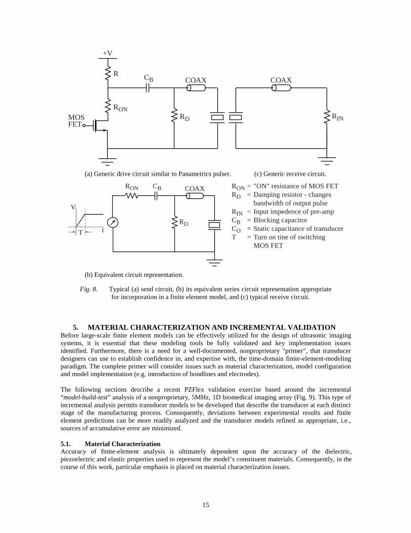
4.5. Electric circuitsUltrasonic transducers are invariably connected to some supporting electronics, frequently through acoaxial cable. During the design process, it is typically necessary to model the drive circuitry, the receptionelectronics and the intervening cable. When designing the electronics, it is most efficient to compute theimpulse response of the transducer and use this in a circuit design code. When looking at the transducerdetails, it is more efficient to model the electronics directly. Fortunately, a few lumped parameter circuitelements (resistors, inductors, capacitors, and ideal transformers) usually suffice. Figure 8 shows genericdrive (send) and receive circuits.
In the time domain approach, electrical boundary conditions on the electrodes are replaced by a coupled setof equations relating the voltage and charge (or their time derivatives) on the electrodes to the voltage andcharge (or their time derivatives) throughout the circuit. The electrical boundary conditions (open, ground,applied voltage or current) then apply to the circuit rather than to the electrode. We note that the chargesand potentials at each of the circuit elements are fully coupled to the nodal values throughout the FE modelat each timestep. Careful algorithmic design is required to solve this system accurately and efficiently.
Electrodes themselves are typically modeled as voltage constraints, i.e., the voltage on each electrode nodeis constrained to be equipotential. This is almost always an accurate approximation, though windowingcould be accounted for if need be and so can unusual electrical resistance. The mechanical effects ofelectrodes are typically neglected too. The electrode mass and stiffness could be accounted for, but they areusually negligible when compared to those of the ceramic.
15
CB COAX
MOSFET
+V
R
RONRD
COAX
RIN
(a) Generic drive circuit similar to Panametrics pulser. (c) Generic receive circuit.
CB COAXRON
RDtT
V
RON = "ON" resistance of MOS FETRD = Damping resistor - changes
bandwidth of output pulseRIN = Input impedence of pre-ampCB = Blocking capacitorCO = Static capacitance of transducerT = Turn on tine of switching
MOS FET
(b) Equivalent circuit representation.
Fig. 8. Typical (a) send circuit, (b) its equivalent series circuit representation appropriatefor incorporation in a finite element model, and (c) typical receive circuit.
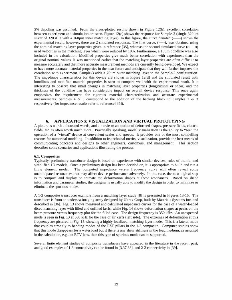
5. MATERIAL CHARACTERIZATION AND INCREMENTAL VALIDATIONBefore large-scale finite element models can be effectively utilized for the design of ultrasonic imagingsystems, it is essential that these modeling tools be fully validated and key implementation issuesidentified. Furthermore, there is a need for a well-documented, nonproprietary "primer", that transducerdesigners can use to establish confidence in, and expertise with, the time-domain finite-element-modelingparadigm. The complete primer will consider issues such as material characterization, model configurationand model implementation (e.g. introduction of bondlines and electrodes).
The following sections describe a recent PZFlex validation exercise based around the incremental“model-build-test” analysis of a nonproprietary, 5MHz, 1D biomedical imaging array (Fig. 9). This type ofincremental analysis permits transducer models to be developed that describe the transducer at each distinctstage of the manufacturing process. Consequently, deviations between experimental results and finiteelement predictions can be more readily analyzed and the transducer models refined as appropriate, i.e.,sources of accumulative error are minimized.
5.1. Material CharacterizationAccuracy of finite-element analysis is ultimately dependent upon the accuracy of the dielectric,piezoelectric and elastic properties used to represent the model’s constituent materials. Consequently, in thecourse of this work, particular emphasis is placed on material characterization issues.

16
1
Inner matching layer
Backing
Outer matching layer
2 3 4 5 44 45 46 47 48
PZT
Fig. 9. Diagram of validation array assembly (2 PZT slivers per physical array element)
Piezoceramic properties are obtained via the application of curve-fitting techniques to IEEE standardresonator measurements [31]. The material properties are then cross-checked by comparing theexperimental impedance responses for the IEEE standard resonators with the corresponding PZFlexpredictions. In the work described here, matching layer and backing properties were obtained via acombination of through-transmission water tank measurements [32] and measurements made with a pair ofcontact shear-wave probes. Unfortunately, these measurement methods have several distinct drawbacks andhence, more comprehensive and accurate measurement schemes are currently being developed [33].
Piezoceramic Characterization: The IEEE standard on piezoelectricity [34] identifies certain geometricalshapes that may be used to facilitate the measurement of a material’s elastic, dielectric and piezoelectricproperties. For piezoelectric materials, there are 5 standard resonator geometries (Fig. 10). These resonatorsamples are specifically designed so as to isolate certain types of resonant behavior. Consequently, it ispossible to measure those material properties that are strongly coupled to a particular resonant mode. Theequations used to determine the material properties (as given in the IEEE piezoelectric standard [34]) haveidealized derivations, and assume that the material is lossless. In practice, all real materials possess certainloss mechanisms, and hence the calculated properties will be subject to certain inaccuracies. A refinementto this method has been developed by researchers at the Royal Military College of Canada and employscurve-fitting techniques to more accurately determine a material’s properties. The software package, PRAP[31], was used to perform this analysis and the extracted material properties for Motorola 3203HD PLZTare given in reference [35].
The IEEE resonators shown in Figure 10 were modeled in PZFlex using the measured properties given in[35]. Figures 11a-11d show the correlation between the experimental electrical impedance response andthe corresponding PZFlex predictions for a selection of these resonator samples. In all cases, PZFlex is seen
(a) Thickness extensional mode (TE) (b) Length extensional mode (LE) (c) Radial mode (RAD)
(d) Length thickness mode (LTE) (e) Thickness shear mode (TS)
Fig. 10. IEEE standard piezoelectric resonators:(a) TE, (b) LE, (c) RAD, (d) LTE, (e) TS.

17
(a) 3.0 3.5 4.0 4.5 5.0 5.5 6.0
Frequency (MHz)
100
101
102
103
104
Mag
nitu
de (
Ohm
s)
PZFlexExperimental
(b)0.0 0.2 0.4 0.6 0.8
Frequency (MHz)
103
104
105
106
107
108
Mag
nitu
de (
Ohm
s)
PZFlexExperimental
(c)0.0 0.5 1.0 1.5 2.0
Frequency (MHz)
100
101
102
103
104
105
Mag
nitu
de (
Ohm
s)
PZFlexExperimental
(d)0.0 0.2 0.4 0.6 0.8 1.0
Frequency (MHz)
102
103
104
105
Mag
nitu
de (
Ohm
s)
PZFlexExperimental
Fig. 11. Impedance magnitude response for resonators: (a) TE (upper left), (b) LE (upperright), (c) RAD (lower left), and (d) LTE (lower right).
to demonstrate excellent correlation with experimental results. The simulated in-air impedance responsefor the thickness extensional mode resonator (TE) correctly predicts the spurious modal activity lyingbetween the electrical resonance at 4.1MHz and the mechanical resonance at 4.7MHz (Fig. 11a). Thesespurious resonances are due to lateral modes that are supported by the resonator’s physical geometry. Ifthese parasitic modes are too strongly coupled to the particular resonance of interest, the extracted materialproperties will be inaccurate. The TE resonator used in the current work effort was specifically chosen suchthat its dimensions fully satisfy the guidelines laid down in the IEEE piezoelectric standard. Since the otherresonators have greater modal separation, their impedance response curves appear cleaner and moreunimodal.
It is important to note that a given set of IEEE standard resonators will provide material properties that
were measured over a range of different frequencies. For example, the TE resonator provides Dc33 at
4.7MHz whereas the LTE resonator yields d13 at 200kHz. Typically, all material properties will exhibitsome degree of frequency dependence, however, with care, it is possible to select a set of properties thatgive consistent results over a wide range of frequencies.
Matching Layer and Backing Block Characterization: The validation array considered in this paper has adouble matching layer and light acoustic backing attached to its upper and lower surfaces respectively (seeFigure 9). Accurate characterization of these passive materials is just as important as for the piezoceramic.The material properties that need to be measured are longitudinal-wave velocity & attenuation, and shear-wave velocity & attenuation. Longitudinal velocity and attenuation measurements are relativelystraightforward and may be accomplished via a simple through-transmission experiment. Unfortunately,measurement of the shear properties is typically much more difficult and potentially less accurate. Shearproperties are normally obtained by attaching a pair of shear wave transducers to opposite sides of a testspecimen and propagating a shear wave through the sample. Unfortunately, it often proves difficult to getgood coupling of energy between the transducers and the sample. Consequently, the measured values aresubject to considerable inaccuracies. Furthermore, these measurements are typically narrowband so resultsare only valid over a narrow range of frequencies. Wu at the University of Vermont is currently refining awide-band, through-transmission, water tank characterization technique [33] for passive isotropic materials.It provides both velocity and attenuation data over a wide range of frequencies. Until material properties

18
obtained via this method become available, the characterization techniques described in [32] will be used tocharacterize the array’s matching layer and backing block materials (see reference [35] for measuredmaterial properties).
5.2. PZFlex Validation – Incremental Array SamplesOnce all the active and passive materials have been accurately characterized, it is feasible to proceed withPZFlex analysis of the transducer array assembly shown in Figure 9. This array is constructed fromMotorola 3203HD PLZT and has 48 individual elements, each comprising two sub-elements as shown inFigure 9. A double layered, sub-diced matching layer was adopted and a “light” acoustic backing(Z|2.5Mrayl) was bonded to the bottom of the device to help improve bandwidth characteristics whilemaintaining reasonable transmit sensitivity. For validation purposes, rather than attempting to model theentire array assembly, the analysis is currently restricted to the set of incremental array components shownin Figure 12(a). Each sample corresponds to half an individual array element, and was fabricated using thesame techniques used to construct the complete array. Consequently, any process dependent effects shouldalso be observed in the incremental samples.
The first step of the validation exercise is to confirm that the PZFlex prediction for each of these sub-unitsagrees with experimental values. Figure 12(b) shows both the experimental (——) and simulated (o·····o)electrical impedance response curves for Sample-1. At various stages throughout the fabrication process thepiezoceramic slivers are subject to elevated temperatures and other process effects. These conditions causethe piezoceramic to partially depole, i.e. its piezoelectric coupling constants will be reduced. Consequently,
(a)
320µm
160µm
70µm
1 2 3 5
3203HD PZT
Inner matching layer
Backing
Outer matching layer
750µm
135µm 135µm
4
Element length = 8mm
135µm135µm135µm (b)2.0 4.0 6.0 8.0 10.0
Frequency (MHz)
100
101
102
103
104
105
Mag
nitu
de (
Ohm
s)
PZFlex Experimental
(c) 2.0 4.0 6.0 8.0 10.0
Frequency (MHz)
100
101
102
103
104
105
Mag
nitu
de (
Ohm
s)
PZFlex (nominal properties)PZFlex (modified properties)Experimental
(d)2.0 4.0 6.0 8.0 10.0
Frequency (MHz)
100
101
102
103
104
105
Mag
nitu
de (
Ohm
s)
PZFlex (nominal properties)PZFlex (modified properties)Experimental
Fig. 12. (a) Diagram of incremental array components with sample numbers shown, andelectrical impedance response for (b) Sample-1, (c) Sample-2, and (d) Sample-3.
19
5% depoling was assumed. From the cross-plotted results shown in Figure 12(b), excellent correlationbetween experiment and simulation are seen. Figure 12(c) shows the response for Sample-2 (single 320µmsliver of 3203HD with a 160µm inner matching layer). In this figure, the curve denoted (——) shows theexperimental result, however, there are 2 simulated responses. The first curve, (-----), was obtained usingthe nominal matching layer properties given in reference [35], whereas the second simulated curve (o·····o)used velocities in the matching layer which were reduced by 10%. Furthermore, a 10µm bondline was alsoincluded in the calculation. Modified properties give much better correlation with experiment than theoriginal nominal values. It was mentioned earlier that the matching layer properties are often difficult tomeasure accurately and that more accurate measurement methods are currently being developed. We expectto have more accurate material properties in the near future and anticipate that they will further improve thecorrelation with experiment. Sample-3 adds a 70µm outer matching layer to the Sample-2 configuration.The impedance characteristics for this device are shown in Figure 12(d) and the simulated result withbondlines and modified material properties is seen to compare well with the experimental result. It isinteresting to observe that small changes in matching layer properties (longitudinal or shear) and thethickness of the bondline can have considerable impact on overall device response. This once againemphasizes the requirement for rigorous material characterization and accurate experimentalmeasurements. Samples 4 & 5 correspond to the addition of the backing block to Samples 2 & 3respectively (for impedance results refer to reference [35]).
6. APPLICATIONS: VISUALIZATION AND VIRTUAL PROTOTYPINGA picture is worth a thousand words, and a movie or animation of deformed shapes, pressure fields, electricfields, etc. is often worth much more. Practically speaking, model visualization is the ability to “see” theoperation of a “virtual” device at convenient scales and speeds. It provides one of the most compellingreasons for numerical modeling. In addition to its technical merits, visualization, provide the best means ofcommunicating concepts and designs to other engineers, customers, and management. This sectiondescribes some scenarios and applications illustrating the process.
6.1. CompositesTypically, preliminary transducer design is based on experience with similar devices, rules-of-thumb, andsimplified 1D models. Once a preliminary design has been decided on, it is appropriate to build and run afinite element model. The computed impedance versus frequency curve will often reveal someunanticipated resonances that may affect device performance adversely. In this case, the next logical stepis to compute and display or animate the deformation shapes at these resonances. Based on shapeinformation and parameter studies, the designer is usually able to modify the design in order to minimize oreliminate the spurious modes.
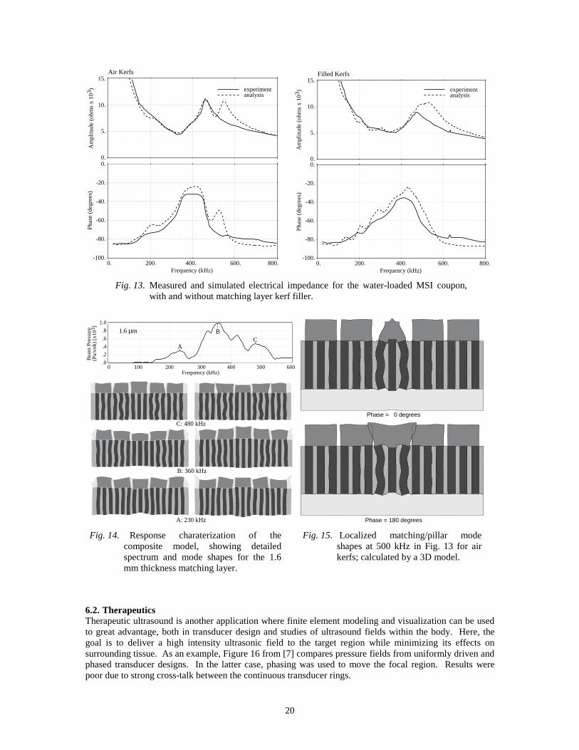
A 1-3 composite transducer example from a matching layer study [8] is presented in Figures 13-15. Thetransducer is from an undersea imaging array designed by Ultrex Corp, built by Materials Systems Inc. anddescribed in [36]. Fig. 13 shows measured and calculated impedance curves for the case of a water-loadeddiced matching layer with filled and unfilled kerfs, while Fig. 14 shows deformation shapes at peaks on thebeam pressure versus frequency plot for the filled case. The design frequency is 350 kHz. An unexpectedmode is seen in Fig. 13 at 500 kHz for the case of air kerfs (left side). The extremes of deformation at thisfrequency are pictured in Fig. 15, showing a highly localized, matching layer mode. This is a lateral modethat couples strongly to bending modes of the PZT pillars in the 1-3 composite. Computer studies showthat this mode disappears for a water load but if there is any shear stiffness in the load medium, as assumedin the calculation, e.g., an RTV lens, then this type of spurious mode can be supported.
Several finite element studies of composite transducers have appeared in the literature in the recent past,and good examples of 1-3 connectivity can be found in [3,37,38], and 2-2 connectivity in [39].
20
0.
5.
10.
15.
Am
plitu
de (
ohm
s x
103)
0. 400. 200. 800.600. -100.
-80.
-60.
-40.
-20.
0.
Frequency (kHz)
Pha
se (
degr
ees)
experimentanalysis
Air Kerfs
0.
5.
10.
15.
Am
plitu
de (
ohm
s x
103)
0. 400. 800.200. 600. -100.
-80.
-60.
-40.
-20.
0.
Frequency (kHz)
Pha
se (
degr
ees)
experimentanalysis
Filled Kerfs
Fig. 13. Measured and simulated electrical impedance for the water-loaded MSI coupon,with and without matching layer kerf filler.
A: 230 kHz
B: 360 kHz
C: 480 kHz
0 200100 500400300 600 .0
.2
.4
.6
1.0
.8
Frequency (kHz)
Bea
m P
ress
ure
(Pa/
volt)
[x10
3 ] 1.6 µm
A
BC
Phase = 0 degrees
Phase = 180 degrees
Fig. 14. Response charaterization of thecomposite model, showing detailedspectrum and mode shapes for the 1.6mm thickness matching layer.
Fig. 15. Localized matching/pillar modeshapes at 500 kHz in Fig. 13 for airkerfs; calculated by a 3D model.
6.2. TherapeuticsTherapeutic ultrasound is another application where finite element modeling and visualization can be usedto great advantage, both in transducer design and studies of ultrasound fields within the body. Here, thegoal is to deliver a high intensity ultrasonic field to the target region while minimizing its effects onsurrounding tissue. As an example, Figure 16 from [7] compares pressure fields from uniformly driven andphased transducer designs. In the latter case, phasing was used to move the focal region. Results werepoor due to strong cross-talk between the continuous transducer rings.

21
Axial P (MPa)0o Phase Delay 72o Phase Delay
P (MPa)0 .4 .8 1.2 0 .2 .4 .6
Vitreous Humor (Water) Fatty Tissue (T2)
Ultrasound Field(Steady State)
Temperature Field(at 3 seconds)
Melanoma (T1)
105
94.7
84.2
78.9
68.4
58.0
47.5
37.0
Tem
pera
ture
(o C)
Fig. 16. Calculated field and on-axis pressurefrom a radially poled, 2 mm thick, PZT-5H spherical cap with 10 cm apertureand radius (f/1). Ten equal-area annularelectrodes are driven by 1.0 volt at 1.0MHz, uniformly (left) or phased (right).
Fig. 17. Axisymmetric model of an oculartumor, showing focused ultrasound beam(above) and temperature distribution at 3sec (below). Note focal temperature inexcess of 100 °C. The transducer has a 4cm aperture and 9 cm focal length.
Because of high intensities at the focus, material nonlinearities in tissue become an issue. These includeboth compressive nonlinearity that is commonly described by the first nonlinear term (B/A) in an expansionof the pressure density relation, and cavitation under tensile stresses. Both of these are readily modeled inthe time domain [7]. We note that material nonlinearity causes the generation of higher harmonics.Damping in tissue increases with increasing frequency, so these in turn induce greater losses andconsequently higher heat generation. At extremely high intensities such as those found in lithotripsy, or atvery long propagation distances, shock phenomena must also be modeled.
Transducer and wave field calculations are sometimes the means rather than the end of a simulation [7].Figure 17 shows the computed pressure field (upper half) near the focus of a therapeutic ultrasoundtransducer. From this we calculate the thermal heat generation per unit time at each point in the model andthen solve the bioheat equations for evolution of temperature with time. Temperature at 3 seconds is shownin the lower half of the figure. High temperatures can be used to destroy diseased tissue, but collateraldamage to healthy tissue by thermal or cavitation mechanisms should be minimized. Simulations provide aconvenient method to refine treatment strategies prior to in vivo validations on laboratory animals.
6.3 PrototypingA last example is used to illustrate virtual prototyping of transducers. Fig. 18 shows a 3D model of aTonpilz device for low frequency sensing in air. This classical design is usually used for water-loadedapplications. The model consists of a tail-mass, a stack of four PZT rings, and a conical head-mass, all heldtogether by a tension bolt through the axis. A thick matching layer with stiffening ring is bonded to thehead mass.
One issue of interest for nominally axisymmetric devices is bending modes caused by nonsymmetricinfluences. One common influence is nonuniform driving by the piezoelectric rings. This was studied byintroducing pseudorandom variation in the coupling constant around each ring. Both impedance andvelocity spectra were examined to identify nonsymmetric modes. The principal bending mode was foundat 7 kHz and shown on the left side of Fig. 18. The principal longitudinal mode was around 14 kHz, shownon the right side of Fig. 18. Higher harmonics of the bending mode were not apparent. Effects of mountlocations and nonsymmetric mounting fixtures were also studied. Such analyses are readily done withnumerical models and tend to reduce the need for an exhaustive set of prototype devices. Nonetheless,validation against experiment is mandatory.

22
xy
z
xy
z
Fig. 18. Examples of bending (left) and longitudinal (right) modes of an air-coupledTonpilz transducer. A thick, flexible matching layer is bonded to the face of theconical head-mass.
7. CONCLUSIONSThis paper was intended as a primer on various issues pertinent to finite element modeling of ultrasonictransducers. The breadth of the topic is vast and multi-disciplinary in nature, and this overview is perforceselective. We have attempted to review the basic algorithmic background and practical modeling issues tothe extent they affect simulation strategies and capabilities. We have also tried to convey the idea thatmodeling is not an exercise independent of experimentation, whether to determine the requisite materialproperties or to develop intuitive understanding of the transducer's operational parameters. Much can bedone to improve the accessibility of advanced simulation techniques, through intuitive graphical interfaces,standardized design "templates", and robust algorithms that require less interaction between the end-userand the "numerics". We do not foresee however that increased accessibility renders obsolete efforts todevelop modeling skills and basic understanding of the underlying analytical methods. From our currentperspective at least, these often effectively complement design skills: a good model reflects a goodunderstanding of the physics.
8. ACKNOWLEDGEMENTSThis work was supported in parts under NSF SBIR Grant DMI-9313666, NIH SBIR Grant 1R43CA65255,and several ONR or DARPA/ONR contracts. We gratefully acknowledge the support and encouragementof our ONR monitors Dr. W.A. Smith and Mr. S. Littlefield. Various studies here mentioned wereundertaken in collaboration with Dr. C. DeSilets of Ultrex Corp, Materials Systems Inc., Hewlett Packard,the Royal Military College of Canada, the Naval Undersea Warfare Center, UDI-Fugro Ltd., TheUltrasonics Group at the University of Strathclyde, the Riverside Research Institute and others, all of whichwe are grateful for.

23
9. REFERENCES1. H. Allik and T.J.R. Hughes, "Finite element method for piezoelectric vibration", Int. J. Num. Meth.
Engng., Vol. 2(2), pp. 151-157, 1970.2. H. Allik, K.M. Webman and J.T. Hunt, "Vibrational response of sonar transducers using piezoelectric
finite elements", J. Acoust. Soc. Am., Vol. 56, 1782-1792, 1074.3. J.A. Hossack and G. Hayward, "Finite element analysis of 1-3 composite transducers", IEEE Trans.
Ultrason., Ferroelect., Freq. Contr., Vol. 38(6), pp 91, 1991.4. R. Lerch, "Simulation of piezoelectric devices by two- and three-dimensional finite elements", IEEE
Trans. Sonics Ultrason., Vol. SU-37, 233-247, 1990.5. G.L. Wojcik, D.K. Vaughan, N.N. Abboud and J. Mould, “Electromechanical modeling using Explicit-
time-domain finite elements,” Proc. IEEE Ultrason. Symp., 2, 1107-1112, 1993.6. G.L. Wojcik, D.K. Vaughan, V. Murray and J. Mould, “Time-domain modeling of composite arrays
for underwater imaging,” Proc. IEEE Ultrason. Symp., 1994.7. G.L. Wojcik, J. Mould, F. Lizzy, N.N. Abboud, M. Ostromogilsky and D.K. Vaughan, “Nonlinear
modeling of therapeutic ultrasound,” Proc. IEEE Ultrason. Symp., 1617-1622, 1995.8. G.L. Wojcik, C. DeSilets, L. Nikodym, D.K. Vaughan, N.N. Abboud and J. Mould, “Computer
modeling of diced matching layers” Proc. IEEE International Ultrason. Symp., 1996.9. G.L. Wojcik, J. Mould, D. Tennant, R. Richards, H. Song, D.K. Vaughan, N.N. Abboud and D.
Powell, “Studies of broadband PMN transducers based on nonlinear models” Proc. IEEE InternationalUltrason. Symp., 1997.
10. G.L. Wojcik, B. Fornberg, R. Waag, L. Carcione, J. Mould, L. Nikodym and T. Driscoll,“Pseudospectral methods for large-scale bioacoustic models” Proc. IEEE International Ultrason.Symp., 1997.
11. N.N. Abboud, J. Mould, G.L. Wojcik, D.K. Vaughan, D. Powell, V. Murray and C. MacLean,"Thermal generation, diffusion and dissipation in 1-3 piezocomposite sonar transducers: finite Elementanalysis and experimental measurements” Proc. IEEE International Ultrason. Symp., 1997.
12. S. Przemieniecki, Theory of Matrix Structural Analysis, Dover Publications, Inc., 1968.13. B.A. Auld, Acoustic Fields and Waves in Solids, Vol. 1, 2nd ed., Krieger Publishing Co., 1990.14. R.H. Burkhart and D.P. Young, "GMRES acceleration and optimization codes", ETA-TR-88, Boeing
Computer Services, May 1988.15. R.W. Freund, "Conjugate gradient type methods for linear systems with complex symmetric
coefficient matrices", SIAM J. Sci. Stat. Comput., Vol. 13(1), 1992.16. R. Courant, K.O. Friedrichs, and H. Lewy, "Über die partiellen differenzengleichungen der
mathematischen physik", Math. Ann., Vol. 100(32), 1928.17. L. Brillouin, Wave Propagation in Periodic Structures, 2nd edition, Dover, 1953.18. N.N. Abboud and P.M. Pinsky, "Finite element dispersion analysis for the three-dimensional second
order scalar wave equation", Int. J. Num. Meth. Engng., Vol. 35(6), pp. 1183-1218, 199219. Z.P. Bazant and Z. Celep, "Spurious reflection of elastic waves in nonuniform meshes of constant and
linear strain finite elements", Comput. Struct., Vol. 15(4), 451-459, 1982.20. T. Belytschko and R. Mullen, "On dispersive properties of finite element solutions", in Miklowitz et al.
(ed.), Modern Problems in Elastic Wave Propagation, pp. 67-82, Wiley, 1978.21. T. L. Szabo, "Time domain wave equations for lossy media obeying a frequency power law", J.
Acoust. Soc. Am., Vol. 96(1), pp. 491-500, 1994.22. M.G. Wismer and R. Ludwig, "An explicit numerical time domain formulation to simulate pulsed
pressure waves in viscous fluids exhibiting arbitrary frequency power law attenuation", IEEE Trans.UFFC, Vol. 42(6), pp. 1040-1049, 1995.
23. D. Givoli, “Non-reflecting boundary conditions: a review”, J. Comp. Phys., Vol. 94, pp. 1-29, 1991.24. O.C. Zienkiewicz, P. Bettess, T.C. Chiam and C. Emson, “Numerical methods for unbounded field
problems and a new infinite element formulation,” in A.J. Kalinowski (ed.), Computational Methodsfor infinite domain media-structure interaction, AMD Vol. 46, pp. 115-148, ASME, 1981.
25. J.G. Blaschack and G.Z Kriegsmann, “A comparative study of absorbing boundary conditions”, J.Comp. Phys., Vol. 77(1), pp. 109-139, 1988.
26. I.S. Sandler, "A new procedure for wave propagation problems and a new procedure for non-reflectingboundaries", Comp. Meth. Appl. Mech. Eng. "special issue on exterior problems of wave propagation",accepted for publication, 1998.

24
27. R. Clayton and B. Enquist, "Aborbing boundary conditions for acoustic and elastic wave equations",Bull. Seism. Soc. Am., Vol. 67, pp. 1529-1540, 1977.
28. J.-P. Berenger, "A perfectly matched layer for the absorption of electromagnetic waves", J. Comp.Phys., Vol. 144, 185-200, 1994.
29. X. Yuan, D. Borup, J. Wiskin, M. Berggren, R. Eidens, S. Johnson, "Formulation and validation ofBerenger's PML absorbing boundary for the FDTD simulation of acoustic scattering, IEEE Trans.Ultrason., Ferroelect., Freq. Contr., Vol. 44(4), 816-822, 1997.
30. J. Bennett, Development of a finite element modelling system for piezocomposite transducers, Ph.D.dissertation, University of Strathclyde, Glasgow, Scotland, Nov. 1995.
31. PRAP – “Piezoelectric Resonance Analysis Program”, TASI Technical Software, 174 Montreal Street,Kingston, Ontario, Canada, K7K 3G4
32. A.R. Selfridge, “Approximate material properties in isotropic materials”, IEEE Trans. On Sonics andUltrasonics, Vol. SU-32, No. 3, 1985
33. Junru Wu, “Determination of velocity and attenuation of shear waves using ultrasonic spectroscopy”,J. Acoust. Soc. Am., Vol. 99 (5), pp.2871-2875, 1996.
34. IEEE Standard on Piezoelectricity, The Institute of Electrical and Electronic Engineers, 198835. D. J. Powell, G.L. Wojcik, C.S. Desilets, T.R. Gururaja, K. Guggenberger, S. Sherrit and B.K.
Mukherjee, “Incremental ‘Model-Build-Test’ Validation Exercise for a 1-D Biomedical UltrasonicImaging Array”, ” Proc. IEEE International Ultrason. Symp., 1997.
36. C. Desilets, et al., “Composite Curved Linear Array for Sonar Imaging: Construction, Testing, andComparison to FEM Simulations,” Proc. IEEE International Ultrason. Symp., 1997.
37. G. Hayward, J. Bennett, and R. Hamilton, "A theoretical study of the influence of some constituentmaterial properties on the behavior of 1-3 connectivity composite transducers", J. Acoust. Soc. Am.,Vol. 98(4), pp 2187-2196, 1995.
38. G. Hayward and J. Bennett "Assessing the influence of pillar aspect ratio on the behavior of 1-3connectivity composite transducers", IEEE Trans. Ultrason., Ferroelect., Freq. Contr., Vol. 43(1), pp98-108, 1996.
39. D.M. Mills and S.W. Smith, "Combining multi-layers and composites to increase SNR for medicalultrasound transducers", Proc. IEEE International Ultrason. Symp., 1997.