finite element method - naval postgraduate schoolfaculty.nps.edu/jenn/ec4630/femv7.pdf · the wave...
TRANSCRIPT

AY2011v7 1
Finite Element Method (Chapter 3)
EC4630 Radar and Laser Cross Section
Fall 2011
Prof. D. Jenn [email protected]
www.nps.navy.mil/jenn

AY2011v7 2
Naval Postgraduate School Department of Electrical & Computer Engineering Monterey, California
Finite Element Method (FEM)
The finite element method (FEM) is the oldest numerical technique applied to engineering problems. FEM itself is not rigorous, but when combined with integral equation techniques it can yield rigorous formulations. Advantages of FEM:
1. Sparse matrices result (as opposed to MM for which dense matrices result). Sparse matrices allow the application of a wide range of fast matrix solvers.
2. Its application involves discretization of the computational domain, and therefore is
adaptable to a wide range of geometries and material variations.
Traditional applications like civil and mechanical engineering use scalar node basis functions. Vector edge basis functions are more appropriate for electromagnetic problems because
• EM problems require solutions of vector quantities • Volume currents are required, not just surface currents • Continuity and boundary conditions are applied to edges, not just nodes (points) • Spurious solutions occur with nodes

AY2011v7 3
Naval Postgraduate School Department of Electrical & Computer Engineering Monterey, California
FEM Formulation (1)
The figure illustrates the generic problem. The computational region is the enclosed volume, Ω. The vector wave equation is the starting point for the FEM solution
2
( )
mo r o o
r r
f
JE k E jk Z J
E
εµ µ
≡
∇×∇× − = − − ∇×
≡
L
A testing procedure is used similar to the method of moments. Each side is multiplied by a testing (weighting) function, and integrated. Using the inner product notation
Ω•= ∫Ω
dWAWA
,
where
W is the test function and A
a field or current. Ideally, the two sides of the wave equation should be equal and the difference zero. In practice the difference will not be zero, so we minimize the functional
( ) ( ), ,F E E W f W= −
L
METAL
DIELECTRIC
OUTER TERMINATION
SURFACE
So
SdSo Ω
ˆ n

AY2011v7 4
Naval Postgraduate School Department of Electrical & Computer Engineering Monterey, California
FEM Formulation (2)
Green’s first vector identity is used to eliminate the double curl. The result is referred to as the weak form of the wave equation. Testing the weak form gives the following equation:
0)ˆ(1)()( 21 =Ω•+•×∇×−Ω
•−×∇•×∇ ∫∫∫
ΩΩ
dWfdsWEndWEkWE ir
roSr
µε
µ
where 0=if
for scattering problems, but not for antenna problems. The unknown quantity is the electric field, E
. A dual equation can be derived for H
. E
and H
are the total fields ( si HHH
+= and si EEE
+= ). The incident fields are known; the scattered fields are unknown. The numerical solution for the integral equation begins by discretizing the volume into subdomains. The fields will be computed on the boundaries of the subdomains. In the equation for E
, integrals over the PEC portions of the surfaces vanish. If the exterior surface (the terminating boundary) is not PEC then a boundary condition must be imposed. (For scattering problems, there should be no reflection at this boundary because it is merely a computational surface, not a physical surface.)

AY2011v7 5
Naval Postgraduate School Department of Electrical & Computer Engineering Monterey, California
FEM Formulation (3)
The surface integral for the terminating boundary can be handled in several ways:
1. For radiation problems where the source is inside, a perfectly matched layer (PML) can be used just inside of the boundary.
2. The surface integral can be replaced by one that incorporates a general boundary condition.
3. An alternative is to use the method of moments to find the equivalent currents on the outer boundary. However, since the surface currents couple with the fields inside, the MM matrix equation must be solved with the FEM matrix equation.
Example: An infinitely long conducting cylinder (arbitrary cross section) using a PML termination
INTERIOR REGION
METAL BOUNDARY
PERFECTLY MATCHED
LAYER (PML)
DISCRETIZED FREE SPACE
REGION
CYLINDER SURFACE

AY2011v7 6
Naval Postgraduate School Department of Electrical & Computer Engineering Monterey, California
FEM Formulation (4)
For the discretized volume with a total of N subdomains, each with Ne edges, the scattered field can be expanded into a series of basis functions with unknown expansion coefficients,
emE . The field inside subdomain e can be expressed as
E e = Eme W m
e
m=1
Ne∑ (
e = 1,, N )
where the expansion coefficients are determined by solving the matrix equation:
or e e emn m mA E B AE B = =
The overbar is a column vector and the double overbar a two square matrix. The vector and matrix elements are of the form
Ω
•−×∇•×∇∫
Ω
= dWWkWWA en
emro
en
em
emn
r
εµ
21 )()(
∫∫Ω
Ω•
−
×∇×∇−•×∇×= dWEkEdsWEnB e
miroie
mir
em
rdS
εµ µ
21)ˆ(1

AY2011v7 7
Naval Postgraduate School Department of Electrical & Computer Engineering Monterey, California
Perfectly Matched Layers (1)
The electrical characteristics of a material are completely described by complex permittivity and permeability matrices
andxx xy xz xx xy xz
yx yy yz yx yy yz
zx zy zz zx zy zz
ε ε ε µ µ µ
ε ε ε ε µ µ µ µ
ε ε ε µ µ µ
= =
where denotes a matrix. Using this notation, Maxwell’s equations can be written in matrix form. For example,
, etc.x xx x xy y xz zD E D E E Eε ε ε ε= ⇒ = + +
and H j Eω ε∇ × =
Most materials have diagonal permittivity and permeability matrices
0 00 00 0o
ab
c
εε
=
For a homogeneous isotropic medium: cba == .

AY2011v7 8
Naval Postgraduate School Department of Electrical & Computer Engineering Monterey, California
Perfectly Matched Layers (2)
θi
θr θt
REGION 1REGION 2
INTERFACE
n
k t
k r
k i
,o oε µ,r rε µ
θiθi
θrθr θtθt
REGION 1REGION 2
INTERFACE
n n
k tk t
k rk r
k ik i
,o oε µ,r rε µ
Let the permittivity equal the permeability at every point in the material
0 00 00 0o o
ab
c
ε µε µ
= =
As in the standard solution of the plane wave reflection coefficients, the fields are written for the two media and tangential components equated at the boundary. However, the
dispersion relationship must be used to determine under what conditions the reflection coefficients will be zero. The result is1 (see Appendix D.2)
TEcos / coscos / cos
i t
i t
b ab a
θ θθ θ⊥
−Γ = Γ =
+
|| TM/ cos cos
cos / cost i
i t
b ab aθ θ
θ θ−
Γ = Γ =+
1See S. D. Gedney, “An Anisotropic Perfectly Matched Layer-Absorbing Medium for the Truncation of FDTD Lattices,” IEEE Transactions on Antennas & Propagation, vol. 44, no. 12, Dec. 1996.

AY2011v7 9
Naval Postgraduate School Department of Electrical & Computer Engineering Monterey, California
Perfectly Matched Layers (3)
The reflection coefficients will be zero if TM TE= 0a b ⇒ Γ = Γ =
From Snell’s law at the boundary,
sin sin 1t ibc bcθ θ= ⇒ =
Choose jBA
cjBAba−
=−=1and = (A and B are real). A good choice is 1≈= BA .
Features of the PML: 1. It is a reflectionless medium for all frequencies and incidence angles
2. Not physically realizable, but it is used as a termination for computational domains in numerical solutions
3. B controls the absorptivity of the layer 4. The PML represents a perfectly matched uniaxial anisotropic medium

AY2011v7 10
Naval Postgraduate School Department of Electrical & Computer Engineering Monterey, California
Grid Termination Methods (1)
The two most common methods for terminating the computational domain are:
(1) Perfectly Matched Layers (PMLs) – The grid is bounded by a layer of nonreflecting material.
(2) Absorbing Boundary Conditions (ABCs) – A boundary condition is applied to the field at the edge of the grid so that the radiation conditions are satisfied (the transmitted field decays to zero at infinity and no reflection at the computational boundary). ABCs take on various forms and are also referred to as transparent boundary conditions and radiation boundary conditions.
Both can be applied conformally or non-conformally.
CONFORMAL TERMINATION
NONCONFORMAL TERMINATION
SCATTERING BODY
SCATTERING BODY

AY2011v7 11
Naval Postgraduate School Department of Electrical & Computer Engineering Monterey, California
Grid Termination Methods (2)
INTERIOR REGION
METAL BOUNDARY
PERFECTLY MATCHED
LAYER (PML)
DISCRETIZED FREE SPACE
REGION
CYLINDER SURFACE
The grid can be terminated by a perfectly matched layer with a metal backing. The thickness and loss of the layer are determined so that the reflections from it are negligible.
• This approach is convenient but requires additional nodes in the computational domain (i.e., the nodes inside of the PML)
• Typical values are εr = µr =1− j and PML thickness d = 0.15λo • The closest points on the target should be 1λo − 2λo from the PML • Conformal layers are preferred because they minimized the number of additional nodes

AY2011v7 12
Naval Postgraduate School Department of Electrical & Computer Engineering Monterey, California
Absorbing Boundary Conditions (1)
The electric and magnetic fields satisfy the vector wave equations
02 =−×∇×∇ ψψ k
where
ψ is either
E or
H . All physically realizable fields must decay to zero at infinity. This is the radiation condition, which can be expressed as
( ) 0ˆlim =−×∇×
∞→ψψ jkrr
r
The fields can be expressed as a series of terms in powers of 1/r (the Wilcox expansion theorem)
1 220
0
( , )( , , )4 4
jkr jkrn
n r rn
e err rr
ψ ψψ θ φψ θ φ ψπ π
− −∞+ + +
=
= =∑
Using the series in the radiation conditions
( ) ∑
××−∇
+−=−×∇×∞
= +••−
0 1)ˆ(ˆ)ˆ()ˆ(ˆ
4ˆ
n nn
jkr
rrrnrr
rrrjk
rejkr ψψψ
πψψ

AY2011v7 13
Naval Postgraduate School Department of Electrical & Computer Engineering Monterey, California
Absorbing Boundary Conditions (2)
If the radiation condition is applied at a finite distance r that is in the far field of the scat-terer, then there is no error. The higher order terms will be forced to zero by equating fields on the boundary. If the boundary condition is applied at a distance r that is in the near field, then the boundary condition is in error. Waves will be set up inside S to match the error terms at the boundary.
E ff =Ke− jkr
r
e− jkr
4πr
ψ 1r
+ψ 2r2 +
ψ 3r3 +
Inside SOutside S
S
Scatterer
In the above example, the error will be on the order of 1/ r2 denoted O(r−2 ). Higher order
boundary conditions can be derived. For example2,
( )( ) ( )( ) 0ˆ/)1(2ˆ tan2
=
−×∇××∏ −−−×∇×
=ψψ jkrrnjkr
N
m
where ( )ψψ ××−= rrtan , satisfies the Nth order condition: O(r−2 N−1). 2 A. Pederson, “Absorbing Boundary Conditions for the Vector Wave Equation,” Microwave & Optical Tech. Lett., vol. 1, pp.62-64.

AY2011v7 14
Naval Postgraduate School Department of Electrical & Computer Engineering Monterey, California
Absorbing Boundary Conditions (3)
Example: For a second order condition the error is O(r−5 ). The exact field at distance r has an infinite number of terms:
= +++
−
221
0exact 4 rr
jkr
re ψψψ
πψ
The boundary condition allows us to retain the terms up to )( 4−rO
( )( )
31 22 3
5 54 44 5 4 5
approx 0
Outgoing waves Fictitious incoming waves
4
4 4
jkr
r r r
jkr jkrA BA B
r r r r
er
e er r
ψψ ψψ ψπ
π π
−+ + +
−+ + + +
=
+ +
Note:
• Low order boundary conditions must be used at large r or significant errors occur. However, this requires a larger computational domain (i.e., more basis functions).
• Higher order boundary conditions can be applied closer to the surface, but are more complex and difficult to implement.
• Note that an increasing number of derivatives are required as the order increases.
AY2011v7 15
Naval Postgraduate School Department of Electrical & Computer Engineering Monterey, California
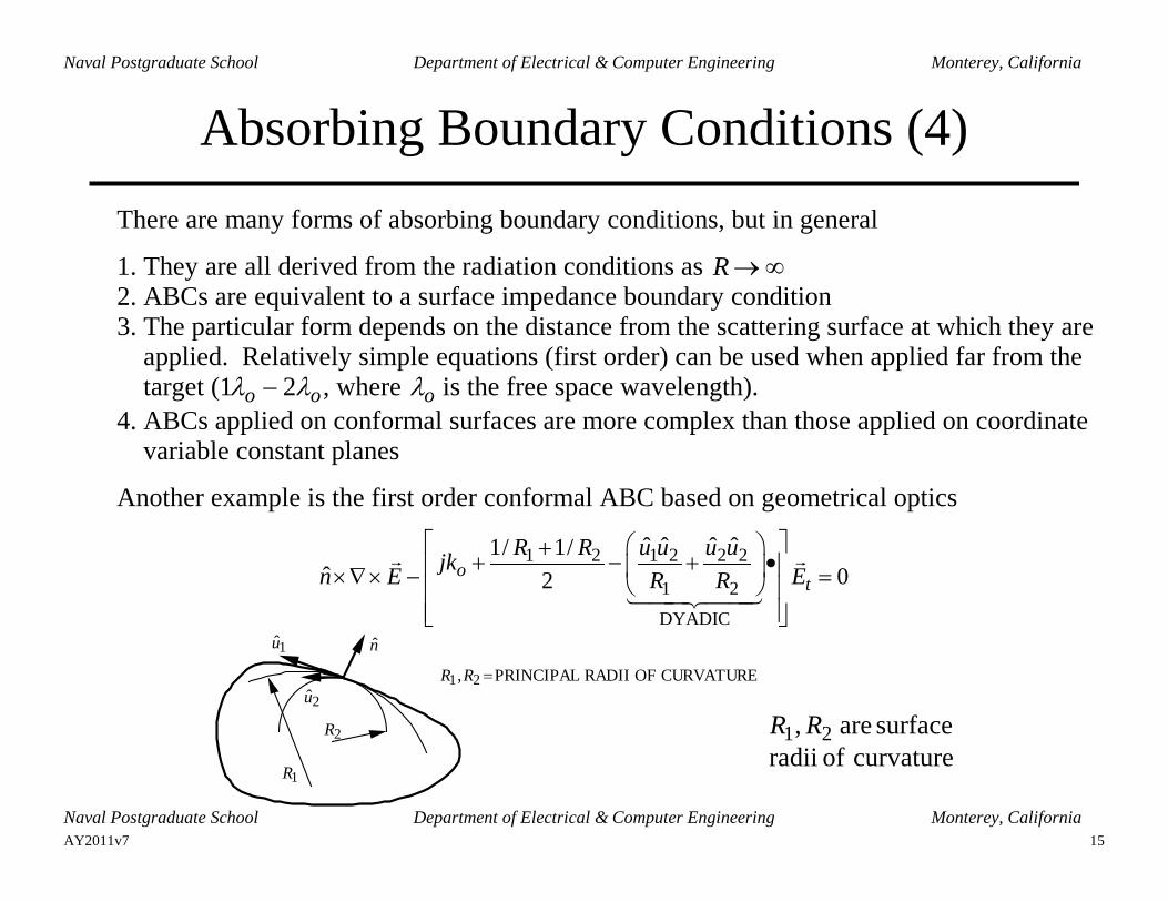
Absorbing Boundary Conditions (4)
There are many forms of absorbing boundary conditions, but in general
1. They are all derived from the radiation conditions as R → ∞ 2. ABCs are equivalent to a surface impedance boundary condition 3. The particular form depends on the distance from the scattering surface at which they are
applied. Relatively simple equations (first order) can be used when applied far from the target ( oo λλ 21 − , where oλ is the free space wavelength).
4. ABCs applied on conformal surfaces are more complex than those applied on coordinate variable constant planes
Another example is the first order conformal ABC based on geometrical optics
1 2 1 2 2 2
1 2DYADIC
ˆ ˆ ˆ ˆ1/ 1/ˆ 02o
t
R R u u u ujkn E ER R +
+ − + • ×∇× − =
ˆ u 1
ˆ u 2
ˆ n
R1
R2
R1,R2 =PRINCIPAL RADII OF CURVATURE
curvature of radiisurface are , 21 RR
Naval Postgraduate School Department of Electrical & Computer Engineering Monterey, California

AY2011v7 16
FEM Subdomains (1)
THREE DIMENSIONAL
TWO DIMENSIONAL
RECTANGLES
TRIANGLES
BRICKS PRISMS
TETRAHEDRAL
BOX REPRESENTED BY RECTANGULAR BRICKS
Two dimensional subdomains
Three dimensional subdomains
Box represented by rectangular bricks
Infinite cylinder in two dimensions using triangles
Car in three dimensions using rectangular bricks

AY2011v7 17
Naval Postgraduate School Department of Electrical & Computer Engineering Monterey, California
FEM Subdomains (2)
For two-dimensional problems triangular subdomains are used. For triangle e, edge k:
W ke = k (Li
e ∇Lje − Lj
e ∇Lie )
EDGE NODE 1 NODE 2
231
123
123
k i j
L2e =
AREA P31AREA 123
L1e =
AREA P23AREA 123
L3e =
AREA P12AREA 123
P(x,y) IS AN INTERNAL POINT
ke = LENGTH OF EDGE k
x
y
1
3 2
1 2
3
P
1 2
3AREA P23
The edge function for edge n has only a tangential component across edge n and only normal components across the other two edges. The field within triangle e is a superposition of the three edge components
E e = Eke
k =1
3∑
W ke

AY2011v7 18
Naval Postgraduate School Department of Electrical & Computer Engineering Monterey, California
FEM Subdomains (3)
For three-dimensional problems, tetrahedra are generally used
W 1 = 1 L1∇L2 − L2∇L1( )
EXAMPLE: EDGE ELEMENT ASSOCIATED WITH EDGE 1
L2 =VOLUME P234VOLUME 1234
L1 =VOLUME P341VOLUME 1234
1 = LENGTH OF EDGE 1
2
5
4
4
6
3
1
3
2
1 P = POINT AT (x,y, z)
1L
2L
W 1 = 1 L1∇L2 − L2∇L1( )
EXAMPLE: EDGE ELEMENT ASSOCIATED WITH EDGE 1
L2 =VOLUME P234VOLUME 1234
L1 =VOLUME P341VOLUME 1234
1 = LENGTH OF EDGE 1
2
5
4
4
6
3
1
3
2
1 P = POINT AT (x,y, z)
1L
2L
The field associated with edge 6 is shown in the figure. Note that:
1. The field turns around edge 6 (which has endpoints 3 and 4). 2. The field is normal to the planes containing nodes 3 and 4. 3. There is tangential continuity across faces 4. There are six edge elements per tetrahedron. Some may be shared with adjacent
tetrahedra.

AY2011v7 19
Naval Postgraduate School Department of Electrical & Computer Engineering Monterey, California
Plate RCS Using HFSS (1) The Ansoft High Frequency Structures Simulator (HFSS) is used to solve transmission line, antenna, and electromagnetic scattering problems using FEM. It has a powerful graphical user’s interface (GUI) for building structures, assigning excitations, meshing, computational parameters, and post processing.
Setup for a square plate:
• frequency: 7.5 MHz (40 m wavelength)
• plate dimensions: 200 m by 200 m in the x-y plane (5 wavelengths square)
• plate thickness: 0.1 m • radiation box
dimensions: 220 m by 220 m by 40 m

AY2011v7 20
Naval Postgraduate School Department of Electrical & Computer Engineering Monterey, California
Plate RCS Using HFSS (2) HFSS has its own computer-aided design (CAD) interface to define the geometry. Drawing data can also be imported from other CAD software packages. HFSS automatically meshes the target and surrounding computational space (the “radiation box”). Radiation boundary conditions are applied on the surfaces of the radiation box.
Close-up of plate mesh
Close-up of radiation box mesh

AY2011v7 21
Naval Postgraduate School Department of Electrical & Computer Engineering Monterey, California
Plate RCS Using HFSS (3)
Bistatic RCS of the square plate for TM polarized 0=θ incidence.

AY2011v7 22
Naval Postgraduate School Department of Electrical & Computer Engineering Monterey, California
Plate RCS Using HFSS (4)
Bistatic RCS of the square plate for TM polarized 45=θ incidence.

AY2011v7 23
Naval Postgraduate School Department of Electrical & Computer Engineering Monterey, California
Aircraft Model in HFSS
Gripen aircraft model with cylindrical computational boundary
Rendered Aircraft (red is dielectric)

AY2011v7 24
Naval Postgraduate School Department of Electrical & Computer Engineering Monterey, California
Aircraft Bistatic RCS From HFSS
for 90φφσ θ φ= =

AY2011v7 25
Naval Postgraduate School Department of Electrical & Computer Engineering Monterey, California
FEM Summary
• FEM is a frequency domain method
• Advantages include geometric and material adaptability, sparse matrices, and compatibility with other engineering analyses
• Approximate grid termination techniques include
1. Perfectly matched layers – not physically realizable, but good for computational purposes
2. Absorbing boundary conditions – complicated when the ABC is applied close to the target surface; simple when far away, but not “node efficient”
• Rigorous termination of the grid requires solving an integral equation for the surface
currents on the grid boundary using MM (this is referred to as the finite element – boundary integral method, FE-BI)
1. Requires solution of the FEM and MM matrix equations simultaneously 2. The MM partition is dense; the FEM partition is sparse. Therefore the
computational intensity has increased substantially.