finite element analysis of the application of synthetic
TRANSCRIPT

Finite Element Analysis of the Application of Synthetic Fiber Ropes to
Reduce Blast Response of Frames
By
Michael Rembert Motley
Thesis Submitted to the Faculty of the
Virginia Polytechnic Institute and State University
In Partial Fulfillment of the Requirements for the Degree of
MASTER OF SCIENCE
IN
CIVIL ENGINEERING
Approved by:
________________________________
Raymond H. Plaut, Chairman
________________________________
Thomas M. Murray
________________________________
Rakesh K. Kapania
December 2004
Blacksburg, Virginia
Keywords: Blast, Synthetic Fiber Ropes, Frame, Springs, Strain Rate Effects

Finite Element Analysis of the Application of Synthetic Fiber Ropes to
Reduce Blast Response of Frames
by
Michael Rembert Motley
Raymond H. Plaut, Committee Chairman
Civil Engineering
(ABSTRACT)
Blast resistance has recently become increasingly relevant for structural engineers. Blast
loads are created by explosive devices that, upon detonation, create pressure loads that
are much higher than most that a structure would ever experience. While there are many
types of blast loads that are impossible to adequately prepare for, methods are presently
being developed to mitigate these loads. This research investigates the possibility of
using synthetic fiber ropes as a means of blast resistance. This is the third phase of a
multi-stage research endeavor whose goal is to analyze Snapping-Cable Energy
Dissipators (SCEDs) for reducing the effects of large-scale lateral loads.
Finite element models of portal frames were developed using the commercial finite
element program ABAQUS and dynamic models were run for varying blasts and frame
systems. Blast pressures of 100, 2,000, and 4,000 psi were applied to a steel portal frame
and comparisons were made between unbraced frames and frames braced with springs of
different stiffnesses. Additional tests were run to examine the effects of strain rate
dependent yield on the results of the models. Parallel research is being conducted on the
specific material behavior of the synthetic fiber ropes so that the models developed for
this research can be revised for a more accurate determination of the effects of the ropes
on structural systems subjected to blast loads.

iii
Acknowledgements
I would initially like to thank my committee chairman and advisor, Dr. Raymond H.
Plaut. He was vital in the completion of this research and in guiding me in the right
direction throughout the duration of this project and his help is highly appreciated.
Furthermore, I would like to thank the members of my committee, Dr. Thomas M.
Murray and Dr. Rakesh K. Kapania, for their willingness to participate in this research
project.
I would also like to thank those who guided me along the way in the completion of this
project. Sangeon Chun and Hitesh Kapoor were very helpful in the initial phases of
researching the effects of blasts. The collaborations with John Ryan, Paul Taylor, and
Greg Hensley were very helpful in developing an understanding of the finite element
programs. Ronald Shope and Soojae Park were integral in the completion of the models.
I would further like to thank the people that I have met and the friends that I have made
during my time in Blacksburg. I have met too many good friends to name them all here
and they have been very supportive of me as I tried to get used to the area and the snow
and everything else. I would also like to thank those whom I left behind from my days at
The Citadel, students and faculty included. Without their help I could have easily found
myself struggling to succeed rather than pushing myself forward.
Finally, I would like to thank the members of my family who have been behind me every
step of the way. Mom and Dad, Mark and Brad, and everyone else back in Charleston
have supported me through thick and thin and have made my life easier in many different
ways. Most importantly, I would like to thank Melissa, who spent the last 18 months
with me in Blacksburg and made more sacrifices for me during that time than I could
have ever expected.
This research was supported by the National Science Foundation under Grant No. CMS-
0114709, and their support is integral in this process and is greatly appreciated.

iv
Table of Contents
Chapter 1: Introduction and Literature Review…………………………………………..1
1.1 Introduction………………………………………………………………..1
1.2 Literature Review………………………………………………………....2
1.2.1 Blast Load Characteristics………………………………………...2
1.2.2 Structural Response to Blast Loads……………………………….4
1.2.3 Blast Resistance…………………………………………………..6
1.3 Scope of Research………………………………………………………...8
Chapter 2: Computer Models for Finite Element Analysis……………………………..10
2.1 ABAQUS…………………………………………………………….......10
2.1.1 Frame Model……………………………………………………..10
2.1.2 Analysis and Element Type……………………………………...11
2.2 ABAQUS Verification…………………………………………………...13
2.2.1 Static Analysis…………………………………………………...13
2.2.2 Dynamic Analysis………………………………………………..15
Chapter 3: Blast Loads on a Bare Frame………………………………………………..19
3.1 Blast Loads……………………………………………………………….19
3.2 Bare Frame Models………………………………………………………21
3.2.1 Case I – 100 psi blast…………………………………………….22
3.2.2 Case II – 2,000 psi blast………………………………………….22
3.2.3 Case III – 4,000 psi blast…………………………………………23
Chapter 4: Effects of Linear Springs on the Models……………………………………35
4.1 SCEDs Modeled as Springs……………………………………………..35
4.2 Effects of Springs on Displacements……………………………………37
4.2.1 Case II – 2,000 psi blast…………………………………………37
4.2.2 Case III – 4,000 psi blast………………………………………...39
4.3 Effects of Springs on Plasticity Spread………………………………….40

v
Chapter 5: Inclusion of Strain Rate Effects……………………………………………..48
5.1 Strain Rate Effects…………………………………………………….....48
5.2 High Strain Rate Effects on Frame Displacements……………………...49
5.2.1 Case II – 2,000 psi blast…………………………………………49
5.2.2 Case III – 4,000 psi blast………………………………………...51
5.3 High Strain Rate Effects on Material Stresses…………………………..65
5.4 High Strain Rate Effects on Material Plasticity…………………………68
Chapter 6: Nonlinear Springs…………………………………………………………..72
6.1 Nonlinear Spring Properties………………………………………….....72
6.2 Displacement Comparisons……………………………………………..74
6.2.1 Spring Case I – 5 kip/in. bilinear springs and corresponding
nonlinear springs………………………………………………...74
6.2.2 Spring Case II – 20 kip/in. bilinear springs and corresponding
nonlinear springs………………………………………………...76
Chapter 7: Conclusions and Recommendations for Future Research…………………..82
7.1 Summary and Conclusions……………………………………………....82
7.2 Recommendations for Future Research……………………………….....85
References……………………………………………………………………………......87
Appendix A: Calculation of the Necessary Frame Displacement for Transformation of
the Springs from Slack to Taut State…………………………………….90
A.1 Calculation of Global X-Displacement Boundary for Transition Between
Slack and Taut States of the Primary Spring…………………………….91
Appendix B: Sample ABAQUS Input File…………………………………………….92
B.1 4,000 psi Blast on a Frame Braced with 8 kip/in.1.3 Nonlinear Springs with
Strain Rate Effects Included……………………………………………..93

vi
Appendix C: Sample ABAQUS Input File…………………………………………...100
C.1 Comparison of Time Histories of Bilinear and Nonlinear Spring
Forces………………………….………………………………………..101
Vita……………………………………………………………………………………...102

vii
List of Figures Figure 2.1: Model of the portal frame……………………………….…………………11
Figure 2.2: Typical cross-sections……………………………………..……………….11
Figure 2.3: Portal frame mesh taken from ABAQUS………………………………….13
Figure 2.4: Deflection of a W8 x 40 cantilever subjected to a 10-kip concentrated load
on the free end. ………………………………………………………….…14
Figure 2.5: ABAQUS vs. initial theoretical calculation for undamped harmonic
excitation of a portal frame……………………………..……………….…17
Figure 2.6: ABAQUS vs. initial theoretical calculation with 4% increase in lumped
mass for undamped harmonic excitation of a portal frame………………..17
Figure 2.7: ABAQUS vs. initial theoretical calculation with 4% decrease in stiffness for
undamped harmonic excitation of a portal frame………………….............18
Figure 2.8: ABAQUS vs. initial theoretical calculation with 2% increase in lumped
mass and 2% decrease in stiffness for undamped harmonic excitation of a
portal frame………………………………………………………………..18
Figure 3.1: Ideal blast curve used in this research……………………………………..19
Figure 3.2: Representation of the blast load on the frame……………………………..20
Figure 3.3: Location of important nodes in the ABAQUS model……………………..22
Figure 3.4: Deflection time-history of node 405 for a 100 psi blast…………………...25
Figure 3.5: Deflection time-history of node 11405 for a 100 psi blast………………...25
Figure 3.6: Sample of von Mises stress distribution in the portal frame subjected to a
100 psi blast load…………………………………………………………..26
Figure 3.7: Deflection time-history of node 405 for a 2,000 psi blast…………………27
Figure 3.8: Deflection time-history of node 11405 for a 2,000 psi blast………………27
Figure 3.9: Deflection time-history of node 205 for a 2,000 psi blast…………………28
Figure 3.10: Deflection time-history of node 11205 for a 2,000 psi blast………………28
Figure 3.11: Sample of von Mises stress distribution in the portal frame subjected to a
2,000 psi blast load at time t = 10 msec……………………………………29
Figure 3.12: Plastic deformation zones of the portal frame subjected to a 2,000 psi blast
at time t = 0.25 sec…………………………………………………………29

viii
Figure 3.13: Deflection time-history of node 405 for a 4,000 psi blast…………………30
Figure 3.14: Deflection time-history of node 11405 for a 4,000 psi blast………………30
Figure 3.15: Deflection time-history of node 205 for a 4,000 psi blast…………………31
Figure 3.16: Deflection time-history of node 11205 for a 4,000 psi blast………………31
Figure 3.17: Comparison of displacement time-histories at node 205 for different
blasts……………………………………………………………………….32
Figure 3.18: Comparison of displacement time-histories at node 405 for different
blasts……………………………………………………………………….32
Figure 3.19: Sample of von Mises stress distribution in the portal frame subjected to a
4,000 psi blast load at time t = 20 msec……………………………………33
Figure 3.20: Plastic deformation zones of the portal frame subjected to a 4,000 psi blast
at time t = 0.25 sec…………………………………………………………33
Figure 3.21: Bending and equivalent plastic strain at the midspan and the support of the
blast side column subjected to a 4,000 psi blast…………………………...34
Figure 4.1: ABAQUS representation of SCEDs introduced into the frame…………...35
Figure 4.2: Representation of how SCEDs would properly be placed into the frame...36
Figure 4.3: Graph of spring stiffnesses………………………………………………...37
Figure 4.4: Comparison of displacement time histories at node 205 for the frame
subjected to a 2,000 psi blast………………………………………………42
Figure 4.5: Comparison of displacement time histories at node 405 for the frame
subjected to a 2,000 psi blast………………………………………………42
Figure 4.6: Comparison of displacement time histories at node 11205 for the frame
subjected to a 2,000 psi blast………………………………………………43
Figure 4.7: Comparison of displacement time histories at node 11405 for the frame
subjected to a 2,000 psi blast ……………………………………………...43
Figure 4.8: Comparison of displacement time histories at node 205 for the frame
subjected to a 4,000 psi blast………………………………………………44
Figure 4.9: Comparison of displacement time histories at node 405 for the frame
subjected to a 4,000 psi blast………………………………………………44

ix
Figure 4.10: Comparison of displacement time histories at node 11205 for the frame
subjected to a 4,000 psi blast………………………………………………45
Figure 4.11: Comparison of displacement time histories at node 11405 for the frame
subjected to a 4,000 psi blast………………………………………………45
Figure 4.12: Plastic deformation zones of the portal frame braced with 20 kip/in. springs
subjected to a 4,000 psi blast at time t = 0.25 sec…………………………46
Figure 4.13: Displacement time history of node 11405 with no springs for 0 < t < 0.01
sec for a 4,000 psi blast……………………………………………………46
Figure 4.14: Plastic deformation zones of the bare portal frame subjected to a 4,000 psi
blast at time t = 5 msec…………………………………………………….47
Figure 5.1: Dynamic yield strength of the frame material based on strain rate………..49
Figure 5.2: Displacement time-histories with and without the inclusion of high strain
rate effects at node 205 for the frame subjected to a 2,000 psi blast with no
springs……………………………………………………………………..53
Figure 5.3: Displacement time-histories with and without the inclusion of high strain
rate effects at node 405 for the frame subjected to a 2,000 psi blast with no
springs……………………………………………………………………..53
Figure 5.4: Displacement time-histories with and without the inclusion of high strain
rate effects at node 11205 for the frame subjected to a 2,000 psi blast with
no springs………………………………………………………………….54
Figure 5.5: Displacement time-histories with and without the inclusion of high strain
rate effects at node 11405 for the frame subjected to a 2,000 psi blast with
no springs………………………………………………………………….54
Figure 5.6: Displacement time-histories with and without the inclusion of high strain
rate effects at node 205 for the frame subjected to a 2,000 psi blast with 5
kip/in. bilinear springs……………………………………………………..55
Figure 5.7: Displacement time-histories with and without the inclusion of high strain
rate effects at node 405 for the frame subjected to a 2,000 psi blast with 5
kip/in. bilinear springs……………………………………………………..55

x
Figure 5.8: Displacement time-histories with and without the inclusion of high strain
rate effects at node 11205 for the frame subjected to a 2,000 psi blast with 5
kip/in. bilinear springs……………………………………………………..56
Figure 5.9: Displacement time-histories with and without the inclusion of high strain
rate effects at node 11405 for the frame subjected to a 2,000 psi blast with 5
kip/in. bilinear springs…………………………………………………….56
Figure 5.10: Displacement time-histories with and without the inclusion of high strain
rate effects at node 205 for the frame subjected to a 2,000 psi blast with 20
kip/in. bilinear springs…………………………………………………….57
Figure 5.11: Displacement time-histories with and without the inclusion of high strain
rate effects at node 405 for the frame subjected to a 2,000 psi blast with 20
kip/in. bilinear springs…………………………………………………….57
Figure 5.12: Displacement time-histories with and without the inclusion of high strain
rate effects at node 11205 for the frame subjected to a 2,000 psi blast with
20 kip/in. bilinear springs…………………………………………………58
Figure 5.13: Displacement time-histories with and without the inclusion of high strain
rate effects at node 11405 for the frame subjected to a 2,000 psi blast with
20 kip/in. bilinear springs…………………………………………………58
Figure 5.14: Displacement time-histories with and without the inclusion of high strain
rate effects at node 205 for the frame subjected to a 4,000 psi blast with no
springs…………………………………………………………………….59
Figure 5.15: Displacement time-histories with and without the inclusion of high strain
rate effects at node 405 for the frame subjected to a 4,000 psi blast with no
springs…………………………………………………………………….59
Figure 5.16: Displacement time-histories with and without the inclusion of high strain
rate effects at node 11205 for the frame subjected to a 4,000 psi blast with
no springs…………………………………………………………………..60
Figure 5.17: Displacement time-histories with and without the inclusion of high strain
rate effects at node 11405 for the frame subjected to a 4,000 psi blast with
no springs…………………………………………………………………..60

xi
Figure 5.18: Displacement time-histories with and without the inclusion of high strain
rate effects at node 205 for the frame subjected to a 4,000 psi blast with 5
kip/in. bilinear springs……………………………………………………..61
Figure 5.19: Displacement time-histories with and without the inclusion of high strain
rate effects at node 405 for the frame subjected to a 4,000 psi blast with 5
kip/in. bilinear springs……………………………………………………..61
Figure 5.20: Displacement time-histories with and without the inclusion of high strain
rate effects at node 11205 for the frame subjected to a 4,000 psi blast with 5
kip/in. bilinear springs……………………………………………………..62
Figure 5.21: Displacement time-histories with and without the inclusion of high strain
rate effects at node 11405 for the frame subjected to a 4,000 psi blast with 5
kip/in. bilinear springs……………………………………………………..62
Figure 5.22: Displacement time-histories with and without the inclusion of high strain
rate effects at node 205 for the frame subjected to a 4,000 psi blast with 20
kip/in. bilinear springs……………………………………………………..63
Figure 5.23: Displacement time-histories with and without the inclusion of high strain
rate effects at node 405 for the frame subjected to a 4,000 psi blast with 20
kip/in. bilinear springs……………………………………………………..63
Figure 5.24: Displacement time-histories with and without the inclusion of high strain
rate effects at node 11205 for the frame subjected to a 4,000 psi blast with
20 kip/in. bilinear springs………………………………………………….64
Figure 5.25: Displacement time-histories with and without the inclusion of high strain
rate effects at node 11405 for the frame subjected to a 4,000 psi blast with
20 kip/in. bilinear springs………………………………………………….64
Figure 5.26: Stress-strain relationship with and without a dynamic increase factor……65
Figure 5.27: von Mises stresses at time t = 5 msec in the bare frame subjected to a 2,000
psi blast load with rate dependent yielding………………………………...66
Figure 5.28: von Mises stresses at time t = 5 msec in the bare frame subjected to a 4,000
psi blast load with rate dependent yielding………………………………...66
Figure 5.29: von Mises stresses at time t = 5 msec in the frame braced with 20 kip/in.
springs subjected to a 4,000 psi blast load with rate dependent yielding….67

xii
Figure 5.30: Plastic deformation zones of the bare portal frame subjected to a 2,000 psi
blast at time t = 0.25 sec…………………………………………………...69
Figure 5.31: Plastic deformation zones of the portal frame braced with 20 kip/in. springs
subjected to a 2,000 psi blast at time t = 0.25 sec…………………………69
Figure 5.32: Plastic deformation zones of the bare portal frame subjected to a 4,000 psi
blast at time t = 0.25 sec…………………………………………………...70
Figure 5.33: Plastic deformation zones of the portal frame braced with 20 kip/in. springs
subjected to a 4,000 psi blast at time t = 0.25 sec…………………………70
Figure 5.34: Bending and equivalent plastic strain at the midspan and the support of the
blast side column subjected to a 4,000 psi blast, with high strain rate effects
included……………………………………………………………………71
Figure 6.1: Bilinear and nonlinear spring force vs. displacement plots based on bilinear
5 kip/in. spring…….……………………………………………………….73
Figure 6.2: Bilinear and nonlinear spring force vs. displacement plots based on bilinear
20 kip/in. spring……………………………………………………………73
Figure 6.3: Displacement time-histories for 5 kip/in. bilinear springs and corresponding
nonlinear springs for node 205 of the frame subjected to a 4,000 psi
blast………………………………………………………………………...78
Figure 6.4: Displacement time-histories for 5 kip/in. bilinear springs and corresponding
nonlinear springs for node 405 of the frame subjected to a 4,000 psi
blast………………………………………………………………………...78
Figure 6.5: Displacement time-histories for 5 kip/in. bilinear springs and corresponding
nonlinear springs for node 11205 of the frame subjected to a 4,000 psi
blast………………………………………………………………………...79
Figure 6.6: Displacement time-histories for 5 kip/in. bilinear springs and corresponding
nonlinear springs for node 11405 of the frame subjected to a 4,000 psi
blast………………………………………………………………………...79

xiii
Figure 6.7: Displacement time-histories for 20 kip/in. bilinear springs and
corresponding nonlinear springs for node 205 of the frame subjected to a
4,000 psi blast……………………………………………………………...80
Figure 6.8: Displacement time-histories for 20 kip/in. bilinear springs and
corresponding nonlinear springs for node 405 of the frame subjected to a
4,000 psi blast……………………………………………………………...80
Figure 6.9: Displacement time-histories for 20 kip/in. bilinear springs and
corresponding nonlinear springs for node 11205 of the frame subjected to a
4,000 psi blast……………………………………………………………...81
Figure 6.10: Displacement time-histories for 20 kip/in. bilinear springs and
corresponding nonlinear springs for node 11405 of the frame subjected to a
4,000 psi blast……………………………………………………………...81
Figure C.1: Comparison of time histories of 5 kip/in. bilinear and corresponding
nonlinear spring forces for frame subjected to a 4,000 psi blast…………101
Figure C.2: Comparison of time histories of 20 kip/in. bilinear and corresponding
nonlinear spring forces for frame subjected to a 4,000 psi blast…………101

xiv
List of Tables
Table 3.1: Peak reflected pressure at 1 msec for 3,000 lb TNT blasts at varying
standoff distances…………………………………………………………..20
Table 3.2: Location of important nodes in the ABAQUS model……………………...21
Table 4.1: Comparison of the structural behavior of the frame at node 405 with
different bracing spring stiffnesses subjected to a blast load of 2,000 psi…38
Table 4.2: Comparison of the structural behavior of the frame at node 205 with
different bracing spring stiffnesses subjected to a blast load of 2,000 psi…38
Table 4.3: Comparison of the structural behavior of the frame at node 11205 with
different bracing spring stiffnesses subjected to a blast load of 2,000 psi…38
Table 4.4: Comparison of the structural behavior of the frame at node 405 with
different bracing spring stiffnesses subjected to a blast load of 4,000 psi…39
Table 4.5: Comparison of the structural behavior of the frame at node 205 with
different bracing spring stiffnesses subjected to a blast load of 4,000 psi…40
Table 4.6: Comparison of the structural behavior of the frame at node 11205 with
different bracing spring stiffnesses subjected to a blast load of 4,000 psi…40
Table 5.1: Effects of the inclusion of rate dependent yield on the bare frame subjected
to a 2,000 psi blast…………………………………………………………50
Table 5.2: Effects of the inclusion of rate dependent yield on the frame braced with 5
kip/in. springs subjected to a 2,000 psi blast………………………………51
Table 5.3: Effects of the inclusion of rate dependent yield on the frame braced with 20
kip/in. springs subjected to a 2,000 psi blast………………………………51
Table 5.4: Effects of the inclusion of rate dependent yield on the bare frame subjected
to a 4,000 psi blast…………………………………………………………52
Table 5.5: Effects of the inclusion of rate dependent yield on the frame braced with 5
kip/in. springs subjected to a 4,000 psi blast………………………………52
Table 5.6: Effects of the inclusion of rate dependent yield on the frame braced with 20
kip/in. springs subjected to a 4,000 psi blast………………………………52
xv
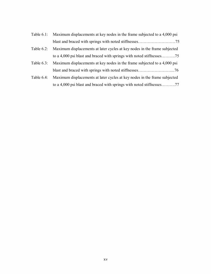
Table 6.1: Maximum displacements at key nodes in the frame subjected to a 4,000 psi
blast and braced with springs with noted stiffnesses………………………75
Table 6.2: Maximum displacements at later cycles at key nodes in the frame subjected
to a 4,000 psi blast and braced with springs with noted stiffnesses……….75
Table 6.3: Maximum displacements at key nodes in the frame subjected to a 4,000 psi
blast and braced with springs with noted stiffnesses……………………...76
Table 6.4: Maximum displacements at later cycles at key nodes in the frame subjected
to a 4,000 psi blast and braced with springs with noted stiffnesses……….77
1
Chapter 1
Introduction and Literature Review
1.1 Introduction
Severe lateral impact loads can cause massive damage to structures and often can result
in complete failure of an entire support structure. Blast loads are among the most
devastating lateral impact loads that a structure may experience. While it is impractical
to design a structure for rare large-scale blasts, engineers are beginning to examine
methods to prevent the failures that can result from more common blasts such as
vehicular bombs. Initial developments in blast resistant design include pressure-
reflecting wall systems and code reevaluation. Many of the innovations for blast design,
however, have been instituted for large or important government buildings with relatively
high budgets. For smaller buildings, other methods of blast resistance must be
developed. Furthermore, affordable methods of retrofit must also be investigated so that
existing buildings can be strengthened for the possibility of a blast.
A multi-stage research endeavor has begun to examine the use of synthetic fiber ropes as
energy dissipators by connecting them diagonally in a slightly relaxed state as a modified
x-brace to structural frames. The initial scope of the research was to analyze the effects
of these ropes as passive earthquake dampers known as snapping-cable energy dissipators
(SCEDs). This research has been expanded to include other possible uses of the ropes.
When a blast occurs, extremely high pressures are exerted upon a structure over a very
short time period. The large peak pressures over small time periods produce dynamic
loads unlike most loads that a structure will experience. These loads, however, can be
extreme in nature and cause high levels of deflection and plastic behavior. The
advantage of these restraints is that they can relieve a structure of some of the deflections
produced by such large dynamic loads that can lead to plastic behavior in the structure.

2
The purpose of this research is to utilize previous research on the SCEDs and on blast
loads and combine those to examine the effects of the SCEDs on structures subjected to
blast loads. The ongoing research includes the examination of the specific dynamic
behavior of the SCEDs as a result of snap loadings. Because this research is not
complete, the SCEDs were modeled as simple springs for a means of comparison. All
modeling of the blast loads was performed in the finite element program ABAQUS.
Models were developed with and without springs so that the spread of plasticity and the
frame deflections could be compared to determine the effectiveness of the springs with
different stiffnesses. Once the actual properties and behavior of the SCEDs are
developed, they can be inserted into the ABAQUS program to determine their exact
effect on the frame.
1.2 Literature Review
1.2.1 Blast Load Characteristics
When an explosive device is detonated, a reaction takes place within the device that
creates extremely high pressures relative to ambient air pressure, and high-speed pressure
waves travel from the center of the blast outward in all directions, gradually decaying
until the waves either completely dissipate or come into physical contact with an object.
The pressures that these objects experience are known as blast loads. The loading
diagram for the pressure of an ideal blast wave can be modeled using the Friedlander
equation (Fung and Chow 1999) defined as
τ
τ
bt
s etptp−
−= 1)(
(1.1)
where ps = peak overpressure;
τ = positive phase duration;
b = decay constant.

3
Furthermore, the characteristics of a specific blast can be defined using the Hopkinson
scaling law (Baker 1973) which states that any two explosions will have the same ideal
blast characteristics at equal scaled distances. The Hopkinson scaling distance is
31
W
RZ =
(1.2)
where R = actual distance from the center of the blast to the point on a structure where
the blast load is applied;
W = weight of the explosive.
Dharaneepathy et al. (1995) examined the distances of explosions from structures and
concluded that there is a “ground-zero distance” for all structures. This distance is the
critical distance where the cumulative blast effects are at a maximum for the specific
structure. Their study was intended to refute the previously held notion that choosing an
arbitrary distance for a blast was adequate for design purposes. They determined that,
particularly for tall structures, the “ground-zero distance” should be used as the design
distance to include the maximum effects of a blast.
An ASCE task committee (Conrath et al. 1999) published a report on designing structures
for physical security that details the relationship between explosive characteristics such
as types, weights, and locations and the resulting pressure loads. In general, blast loads
are characterized in pounds of trinitrotoluene (TNT), a relatively stable chemical
compound that is used in many types of explosives. The pressure of a blast of any type
can be converted to a blast size to be defined in pounds of TNT. Beshara (1994) studied
the modeling of blast loads on above-ground structures and developed mathematical
models used to formulate blast load equations. He explained the conversion of the
energy output of a blast relative to that of TNT using the equation
expexp w
HH
WINT
INT =
(1.3)
where WINT = the equivalent TNT weight;
wexp = the weight of the actual explosive;

4
expH
H INT = TNT equivalent factor (ratio of heat of detonation to heat of explosion).
Williams and Newell (1991) discussed methods for assessing blast response of structures
in a paper written when engineers were just beginning to examine possibilities for blast
resistance. They discussed some of the initial ideas concerning types of blasts and
structural behavior. Blast loads are defined by their incident and reflected overpressures.
Due to the increase in air temperature from the incident wave, reflected blast waves are
multiplied by an amplification factor between 2 and 8, depending on the incident
overpressure. For surface explosions, an amplification factor of 1.8 is used—2.0 factor
less 10% of the explosive energy that goes into cratering.
1.2.2 Structural Response to Blast Loads
Because blast loads occur so much more quickly than most loads and can have much
higher magnitudes than most loads, many types of studies have taken place examining the
effects of blast loads in a range of structural systems. Shope and Plaut (1998,1999)
examined critical blast loads on both one-span and two-span compressed steel columns.
In their first series of analyses on single-span columns, they determined that for a column
subjected to a constant axial load and a uniform blast load, the introduction of residual
stresses and strain-rate effects reduces the maximum axial load at low impulses and
increases the critical impulse at low axial loads. Their later research examined similar
compressed steel columns with two spans. From this work they determined that the
critical impulse for the two-span case is considerably higher than that of single-span
columns of equal length within the acceptable design range.
Williams and Newell (1991) examined the initial concepts of structural response due to
blasts. They explained that when the positive phase duration is much shorter than the
natural period of the structure ( T1.0≤τ ), the blast wave can be assumed to have
produced an instantaneous velocity to the structure, while blasts with longer positive
phase durations ( T6≥τ ) can be treated as static loads. They also stated that as a general

5
rule, materials loaded at high strain rates exhibit higher yield strengths and more ductility
than statically loaded materials. Variations in parameters such as Young’s modulus can
be neglected. For simple SDOF models, for short duration loads it is common to neglect
damping effects because damping can be hard to assess and because, commonly,
damping forces achieve significant magnitude only after substantial motion has occurred.
Barker (1997) discussed dynamic material behavior to aid a task committee formed by
the ASCE Petrochemical Committee. He explained that dynamic material behavior is a
function of material strength as well as deformation, both of which must be taken into
account to properly perform blast analysis and design. Dynamic loads generally produce
an increase in material strength but may decrease ductility. When dynamic loads are
applied to a structural element, the material does not have time to deform at the same rate
as the load is applied. Both yield strength and ultimate strength are affected by this strain
rate behavior. The increase in yield strength can be in the range of 10-40% which can
make a significant difference in blast resistance. Ignoring dynamic effects
underestimates member end reactions, leading to inadequate connection design for the
development of full flexural resistance and prevention of non-ductile failure modes. He
continued by relating that blast design utilizes an ultimate strength approach but
eliminates safety factors on loads since the blast load is assumed to be an infrequent,
maximum load. Resistance factors are also eliminated to reduce conservatism. Structural
elements in blast design are generally allowed to exceed the elastic limit and achieve
plastic deformation, allowing the member to absorb a much larger amount of blast energy
than a static response. Limits on maximum deflection are generally used to determine the
adequacy of a member. The primary deformation parameters are support rotation and
ductility ratio. Support rotation is the angle formed between the longitudinal axis of the
member and a line drawn from the support to the point of maximum deflection. Ductility
ratio is the degree of plasticity achieved in a member. A typical measure of frame
response is sidesway, which is the lateral deflection at the top of the frame relative to the
supports.
Krauthammer (1999) considered the blast resistance of structural concrete and steel

6
connections. He concluded that, in general, the rotational deformation capacities of steel
connections are governed by not only the rigidity of connections, but also the flexural
capacity of the adjoining structural members. For weaker connections, such as in semi-
rigid connections, the rotational capacity of the connection might be governed by its
internal resistance and deformations as opposed to the flexural capacities of the adjoining
members. He also explained that very little emphasis seems to be put on the weak axis
deformations, which results in surprisingly large horizontal deflections. Two major
concerns were developed in the study of structural steel connections, one being the blast
resistance of the connections. It was shown that dead loads have an adverse effect on the
behavior of the connections due to the added bending and twisting of the beams once
they were deformed by the blast.
Longinow and Mniszewski (1996) studied vehicular bombs and their effect on structural
systems. They explained that reflected blast pressures are generally at least twice that of
the incident shock wave and are proportional to the strength of the incident shock, which
is proportional to the weight of the explosive. Developing a structure that will avoid
collapse can be done through the sufficient addition of redundants to effectively
redistribute loads when portions of the structure are destroyed. Effective passive
protection is also crucial for safety, generally in terms of a closed perimeter that prevents
an attack from being close enough to do significant harm to a structure.
1.2.3 Blast Resistance
Events such as the bombing of the Alfred P. Murrah Federal Building in Oklahoma and
the 1993 bombing of the World Trade Centers have brought attention to the need for blast
load retrofitting of existing buildings and blast design standards for new structures.
These events showed that even high-profile structures are not immune to attacks. The
role of the design codes quickly expanded to include blast resistance. Building new
structures to updated blast design specifications, while at times more costly, would be
easier. Cost-effective techniques could be developed for smaller structures. The retrofit

7
of existing structures was an important task for engineers. Several methods were
developed, including reflecting walls and structural dampers.
Mlakar (1996) discussed structural design for vehicular bombs, encouraging a system
exhibiting strength, ductility, and redundancy. The selection bears some resemblance to
the design against strong earthquake motions. An important factor to consider is the
provision for redundant load paths, which can prevent an overall collapse of the structure
with associated catastrophic damage in the event of the destruction of an isolated element
or elements. He also discussed how retrofitting presents a challenging problem for
engineers. While increased standoff distances seem to be the most cost-efficient solution,
it is not always practical. Modification of boundary conditions can result in a stronger
component, for example changing a boundary condition from simply supported to fixed.
Miyamoto et al. (2000) examined blast loadings of 3000 lb of TNT at standoff distances
of 100, 40, and 20 ft. Tests were conducted on a conventional special moment resisting
frame (SMRF) and an SMRF with a fluid viscous damper (FVD). The SMRF is
considered a bare frame and the frame including the damper is a damped frame. For all
cases tested, blast overpressure was assumed to be the most significant cause of failure.
Nonlinear analyses indicated that FVDs provided a cost-effective way to control
displacement and plastic hinge rotation of lateral load resisting frames under blast
loading. FVDs absorb significant amounts of input blast energy throughout the duration
of the structural response. Because maximum displacement occurs at a somewhat late
stage in the time history, damping energy reduces strain energy contribution, thereby
reducing maximum displacement. Large blast loading can overcome kinetic energy and
cause inelastic response in the structure. FVDs can greatly increase the performance of
non-ductile moment frames by eliminating or reducing inelastic demand.
Pearson (2002) and Hennessey (2003) performed the initial research on which this
research is based. They examined the possibility of using snapping-cable energy
disspators for controlling structural response to seismic activity. The unique
accelerations that ground motions induce are similar to the loads produced by blast loads
8
in that they are rare, high-strain-rate events that produce loads much larger than those
seen on a regular basis. Therefore, the use of these cables in blast resistance is examined
in the research herein.
1.3 Scope of Research
The objective of this research is to examine the possible benefits of synthetic fiber ropes
as a means of blast resistance in portal frames. The ropes were modeled as springs in the
finite element analysis program ABAQUS. Bilinear and nonlinear springs were modeled
and the structure was examined with and without the inclusion of rate dependent yield
effects. This research utilizes previous research that was performed on the properties of
the ropes and is part of a multi-stage research project that examines the structural benefits
of Snapping Cable Energy Dissipators (SCEDs).
Chapter two of this thesis discusses the use of the finite element program ABAQUS. The
construction of the frame model is explained and the results of static and dynamic
verification analyses are discussed.
Chapter three begins to examine the effects of blast loads on the portal frame. The
modeling of the blast load in ABAQUS is discussed and key nodes of the frame are
identified. The results of the blast analysis are presented in terms of these key nodes for
the extent of this research.
Chapter four studies the frame with the inclusion of bilinear springs for the same blast
loads as discussed in chapter three. These springs are modeled with some slack in them,
which would be expected in a full-scale model. A comparison of the frame with and
without springs is performed in detail.
Chapter five of this research examines the inclusion of high strain rate effects on the
material behavior of the frame. Comparisons are made between the frames discussed in

9
chapters three and four with and without the addition of rate dependent yield as a material
property.
Chapter six takes information gathered from parallel research regarding the actual
behavior of the springs and analyzes a more realistic model with nonlinear springs.
Comparisons of the nonlinear springs and bilinear springs are made and the benefits of
using particular springs are discussed.
Chapter seven summarizes the entire scope of the research from the previous chapters
and conclusions are made. Recommendations for future research are also made regarding
SCEDs for blast resistance.
Appendix A includes a set of calculations for the length of the springs and the modeling
of the slackness in the ropes. Appendix B contains a series of input files for the
ABAQUS models.
10
Chapter 2
Computer Models for Finite Element Analysis
2.1 ABAQUS
The analysis of a structure’s response to blast loadings is a difficult task. To achieve
adequate results, a multi-degree-of-freedom (MDOF) model must be used with a very
large number of degrees of freedom. An analytical dynamic analysis is suitable for a
model with only a few degrees of freedom. By solving the dynamic equilibrium
equation, an estimate of the structural response can be obtained. There comes a point
where the number of degrees of freedom in a model makes it impractical to derive an
analytical solution. The finite element method is the most practical way to analyze a
structure when a large number of degrees of freedom is necessary. Finite element
analyses can be performed using a number of commercial programs. The finite element
program ABAQUS was used for this research.
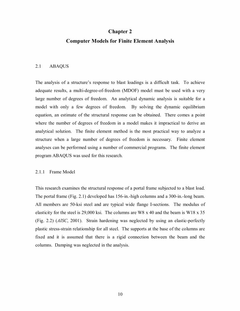
2.1.1 Frame Model
This research examines the structural response of a portal frame subjected to a blast load.
The portal frame (Fig. 2.1) developed has 156-in.-high columns and a 300-in.-long beam.
All members are 50-ksi steel and are typical wide flange I-sections. The modulus of
elasticity for the steel is 29,000 ksi. The columns are W8 x 40 and the beam is W18 x 35
(Fig. 2.2) (AISC, 2001). Strain hardening was neglected by using an elastic-perfectly
plastic stress-strain relationship for all steel. The supports at the base of the columns are
fixed and it is assumed that there is a rigid connection between the beam and the
columns. Damping was neglected in the analysis.

11
Fig. 2.1. Model of the portal frame (base unit = inch)
d tw bf tf A Ix Iy
COLUMN 8.25 0.360 8.07 0.560 11.7 146 49.1BEAM 17.7 0.300 6.00 0.425 10.3 510 15.3
Fig. 2.2. Typical cross-sections (base unit = inch)
2.1.2 Analysis and Element Type
There are several methods of processing a model in ABAQUS. Due to the nature of the
loading, this research used ABAQUS/Explicit as the solver. ABAQUS/Explicit performs
explicit dynamic analyses and is recommended for models with high loads over short

12
time spans. ABAQUS/Explicit uses steps to define the problem history. A step can be
programmed using the *STEP command in an input file. It is at this point that the type of
analysis is defined. This research utilized a dynamic, explicit analysis. Geometric
nonlinearity was considered by specifying an NLGEOM command within the *STEP
portion of the input file.
When performing a finite element model, it is important to determine the proper type of
element for the model that is being analyzed. ABAQUS contains a large number of
different element types, categorized based on family, degrees of freedom, number of
nodes, formulation, and integration. For this research, a C3D8R continuum element was
used. This type of element is an 8-node linear brick with reduced integration. Three-
dimensional brick elements were used to allow for the blast loads to be applied as surface
pressures instead of distributed line loads. ABAQUS recommends using continuum
elements for complex nonlinear analyses involving plasticity and large deformations,
crucial features for blast analysis.
A large number of elements were used to maximize the results. Through an iterative
process it was determined that an adequate model is achieved if the column flanges
contain 720 elements (40 elements high x 9 elements wide x 2 elements deep), the
column webs have 360 elements (40 x 9 x 1), the beam flanges include 1,440 elements
(80 x 9 x 2), and the beam web contains 720 elements (80 x 9 x 1). The mesh can be seen
in Fig. 2.3 taken from ABAQUS.

13
Fig. 2.3. Portal frame mesh taken from ABAQUS
2.2 ABAQUS Verification
The first step in using any commercial software program is the verification of the
modeling technique. For this research, two types of verification were performed. An
initial static deflection analysis for a cantilevered W8 x 40 column with a concentrated
load at the free end was performed to ensure that the continuum elements and the
boundary conditions were properly developed. Second, a single-degree-of-freedom
dynamic analysis was devised as an estimate of the behavior of a frame subjected to a
forced sine wave loading.
2.2.1 Static Analysis
The column used for the static deflection verification was a W8 x 40 with the same input
as the columns in the frame in terms of dimensions, material properties, and elements. A
concentrated load of 10 kips was placed on the end of the column in the local-1 direction.
A static analysis was performed in ABAQUS/Standard—ABAQUS/Explicit is only

14
applicable for dynamic analyses—and the deflections were compared with the equation
for deflection of a cantilevered beam (AISC, 2001):
)23(6
)( 323 lxlxEIPx +−=∆
(2.1)
EIPl3
3
max =∆ (2.2)
where P = concentrated load (kip);
E = modulus of elasticity (ksi);
I = moment of inertia about the bending axis (in.4);
l = total length of the member (in.).
The maximum deflection of the column in ABAQUS was found to be 3.06 in. while the
maximum theoretical deflection is 2.99 in. Fig. 2.4 shows the finite element deflection
and the theoretical deflection of the column.
0
0.5
1
1.5
2
2.5
3
3.5
0 39 78 117 156
x, in.
∆, i
n.
ABAQUS Results Theoretical Results
Fig. 2.4. Deflection of a W8 x 40 cantilever subjected to a 10-kip concentrated load on
the free end.

15
The results from the initial ABAQUS verification coincide with the theoretical results
very closely throughout the length of the column. This verifies that the continuum
elements have been developed such that the boundary conditions and the connections of
the elements are valid.
2.2.2 Dynamic Analysis
The second step of the verification process was ensuring that the dynamic solver was
consistent with theoretical data for a portal frame. The large number of elements and
degrees of freedom in the research model, however, made it unable to perform a parallel
theoretical analysis. Instead, a single-degree-of-freedom (SDOF) analysis was developed
to compare to the ABAQUS analysis. Chopra (2001) explains the process for analyzing
an undamped SDOF frame under harmonic vibration using the equilibrium equation
)sin( tpkuum o ω=+&& (2.3)
where m = mass of the system (kip*sec2/in.);
k = stiffness of the system (kip/in.);
po = maximum value of the force (kip);
ω = forcing frequency (rad/sec);
t = time (sec).
Chopra solves this equation for the displacement, and the resulting equation for a system
beginning at rest, taking into account the complementary and particular solutions, is
−
−= )sin()sin(
)/(11)( 2 tt
kp
tu nnn
o ωωωω
ωω
(2.4)
where ωn = natural frequency of the system (rad/sec).
For the models, a forcing frequency of 100 rad/sec and an amplitude of 300 kips was
used, making the forcing function
)100sin(300)( ttp = (2.5)
A lumped mass, m, of 3.56 lb*sec2/in. was calculated based on the material properties of
the structure and was taken at the midspan of the beam. Chopra also gives an equation

16
for the stiffness of a portal frame based on the relationship between the properties of the
beam and the columns:
41211224
3 ++=
ρρ
c
c
hEI
k (2.6)
where bc
cb
hIhI
=ρ (2.7)
Ic = moment of inertia for the column (in.4);
Ib = moment of inertia for the beam (in.4);
hc = height of the column (in.);
hb = length of the beam (in.);
The stiffness of the system is 23.42 kip/in. The natural frequency of an SDOF system is
calculated as
mk
n =ω (2.8)
Once the variables were calculated and used, the theoretical solution matched the
ABAQUS solution for the first several cycles, then they diverged slightly (Fig. 2.5).
However, because there is such a large difference in the number of degrees of freedom,
some variation is to be expected between the two models. The determination of the mass
and the stiffness would vary between an SDOF model and a model with many degrees of
freedom, thereby changing the natural frequency of the system. Modifications to the
mass and stiffness had a noticeable effect on the theoretical behavior of the system. The
theoretical behavior was examined after raising the mass by 4% (Fig. 2.6), lowering the
stiffness by 4% (Fig. 2.7), and respectively changing both values by 2% (Fig. 2.8). It is
evident that a slight change in those values can make up for the variation in the behavior
calculated by an SDOF model. The frequency with which the structure moves is nearly
identical with the modifications. The difference in amplitude, also seen slightly in the
static deflection test, can be attributed to the fact that the number of integration points is
so high relative to the SDOF model.

17
-60
-40
-20
0
20
40
60
0 0.1 0.2 0.3 0.4 0.5 0.6
time, sec
Beam
Mid
span
Dis
plac
emen
t, in
.
ABAQUS Initial Theoretical Calculation
Fig. 2.5. ABAQUS vs. initial theoretical calculation for undamped harmonic excitation
of a portal frame
-60
-40
-20
0
20
40
60
0 0.1 0.2 0.3 0.4 0.5 0.6
time, sec
Beam
Mid
span
Dis
plac
emen
t, in
.
ABAQUS 4% Mass Change
Fig. 2.6. ABAQUS vs. initial theoretical calculation with 4% increase in lumped mass
for undamped harmonic excitation of a portal frame

18
-60
-40
-20
0
20
40
60
0 0.1 0.2 0.3 0.4 0.5 0.6
time, sec
Beam
Mid
span
Dis
plac
emen
t, in
.
ABAQUS 4% Stiffness Change
Fig. 2.7. ABAQUS vs. initial theoretical calculation with 4% decrease in stiffness for
undamped harmonic excitation of a portal frame
-60
-40
-20
0
20
40
60
0 0.1 0.2 0.3 0.4 0.5 0.6
time, sec
Beam
Mid
span
Dis
plac
emen
t, in
.
ABAQUS 2% Change in Stiffness and Mass
Fig. 2.8. ABAQUS vs. initial theoretical calculation with 2% increase in lumped mass
and 2% decrease in stiffness for undamped harmonic excitation of a portal frame
19
Chapter 3
Blast Loads on a Bare Portal Frame
3.1 Blast Loads
Blast loads are formed when an explosive device is detonated, causing a high speed
pressure wave that creates high pressure loads on a structure over a short time span.
Blasts can be modeled using pressure time histories or as impulses. For this research, the
Friedlander equation (Eq. 1.1) was used. The blast is represented by a unit curve for an
ideal blast load multiplied by varying amplitudes (Fig. 3.1).
-0.2
0
0.2
0.4
0.6
0.8
1
0 0.008 0.016 0.024 0.032
Time, msec
Uni
t Bla
st C
urve
Fig. 3.1. Ideal blast curve used in this research

20
This curve is defined in the input file and then an amplitude is specified in the *STEP
command. The specified amplitude is the peak pressure. All other points on the curve
are based on that value. On the curve, 32 points were calculated at a time step of 1 msec.
Several amplitudes will be applied to this curve to investigate the behavior of the frame.
Miyamoto et al. (2000) examined frames subjected to 3,000 lb TNT blasts at different
standoff distances. Their peak pressures at 1 msec are shown in Table 3.1.
Standoff Distance Peak Reflected Pressure
100 ft 20 psi40 ft 840 psi20 ft 4,400 psi
Table 3.1. Peak reflected pressure at 1 msec for 3,000 lb TNT blasts at varying standoff
distances (Miyamoto and Taylor 2000)
For this research, blasts will be examined with peak pressures of 100 psi, 2,000 psi, and
4,000 psi. Based on the aforementioned study, this is within a realistic range for blast
loads. The load is applied as a lateral pressure along the entire length of the left column
of the frame and acts in the global-X direction throughout its duration; therefore, the
follower effects of the pressure are not taken into account. This can be seen in Fig. 3.2.
Fig. 3.2. Representation of the blast load on the frame
21
To achieve an accurate representation of the effects of the blast on the structure, the time
period of the ABAQUS analysis was 0.25 seconds for each model. This allowed the
structure to experience several cycles of motion before the end of the analysis.
3.2 Bare Frame Models
The purpose of this research is to examine the effects of ropes, modeled as springs, on
frames subjected to blasts with varying peak pressures. The first step of the comparison
is to examine frames without springs. These frames will be referred to as bare frames
throughout the rest of this research. Strain rate effects were ignored for the first series of
models. It is important to note that after all of the models were run, several points were
determined to be key points of deflection in the frame. These points are the midspan of
each column and the top corners of the frame. Nodes were then taken from each area and
used to compare the deflections between different models. These nodes are described in
Table 3.2 and shown in Fig. 3.3.
Node 205 Midspan of blast side column, midpoint of far left flangeNode 405 Top of blast side column, midpoint of far left flange
Node 11205 Midspan of opposite side column, midpoint of far right flangeNode 11405 Top of opposite side column, midpoint of far right flange
Table 3.2. Location of important nodes in the ABAQUS model

22
Fig. 3.3. Location of important nodes in the ABAQUS model
3.2.1 Case I – 100 psi blast
The initial blast applied to the model was a 100 psi blast. This blast caused no permanent
plastic deformation in the structure and little deflection. The deflection of the structure is
small, with a maximum amplitude about 0.2 in. (Figs. 3.4, 3.5). The deflections in these
figures are for nodes 405 and 11405 (see Table 3.2). These small deflections result in
small stresses that do not reach the elastic limit of the material. A model of the von
Mises stresses in the frame can be found in Fig. 3.6. The range of contours in all stress
plots is linear from 0 psi to 50,000 psi. It is noted that there is little change in color in the
100 psi stress diagram as the stresses did not reach high enough values on the applicable
scale. There is some change from the darker blue region of 0 stress to a lighter blue
region that signifies small stress changes in the model.
3.2.2 Case II – 2,000 psi blast
A 2,000 psi blast caused much more drastic results than the 100 psi blast. This blast
caused significant plastic deformation, especially in the blast side column. Analyzing the
results of this model led to the decision that the midpoint of the blast side column (node

23
205) was a crucial point in the behavior of the system. As a means of comparison,
deflection data were collected from the midpoint of the opposite column (node 11205).
The maximum deflection from the 2,000 psi blast was 8.68 in. at node 205, while
deflections only reached 7.21 in. and 7.40 in. at nodes 405 and 11405, respectively (Figs.
3.7, 3.8, 3.9). Fig. 3.10 shows the deflection time-history of node 11205. The slight
variation in deflections at nodes 405 and 11405 can be attributed to two factors—the
location of the nodes on the column and the deflected shape of the frame. The large
deflection at the midspan of the blast side column caused the blast side flange to camber
outward toward the blast, reducing the total deflection at node 405. Likewise, the
bending in the opposite column caused the outer flange to camber outward, increasing
total deflection at node 11405.
Stresses in the frame were analyzed and are shown in Fig. 3.11. The stresses in the frame
for Case II are substantially different from those in Case I. The permanent plastic
deformation in the frame subjected to the 2,000 psi blast is shown in Fig. 3.12. Plastic
deformation was considered to occur when equivalent plastic strain occurred in the
frame. As the blast passed over the frame, plasticity developed initially at the midspan of
the blast side column, at the supports, and at the connections. As the load decayed, the
plasticity spread to its final permanent distribution.
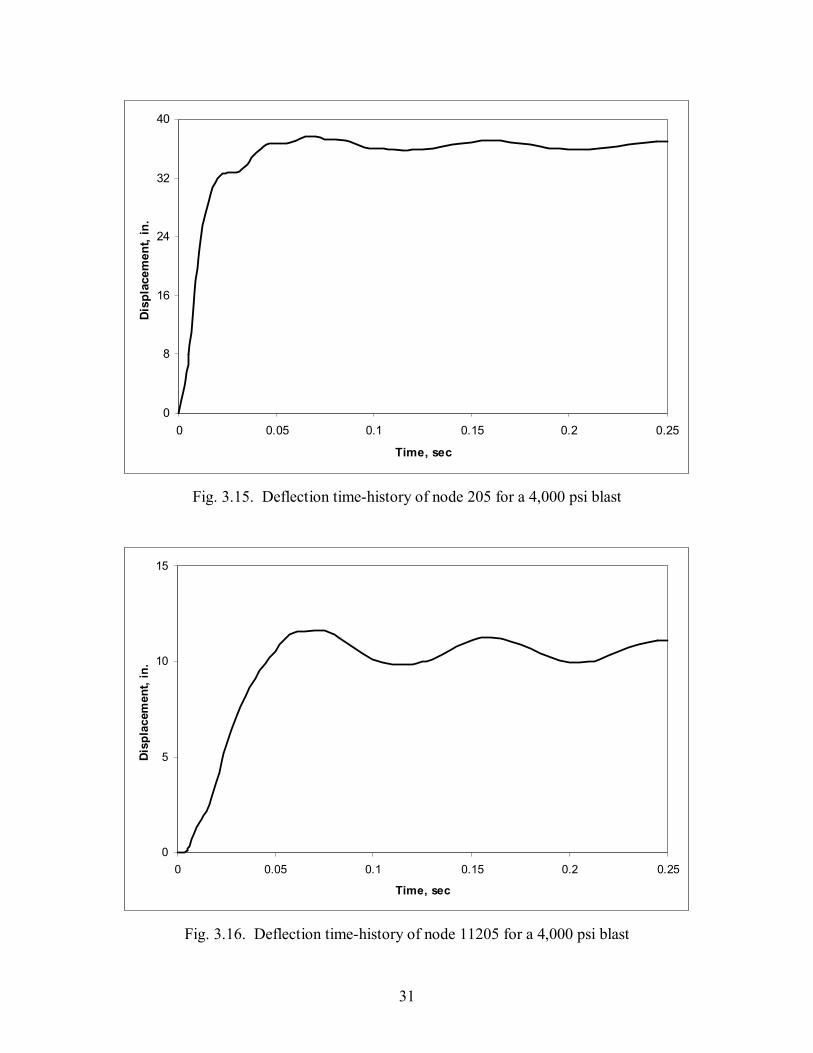
3.2.3 Case III – 4,000 psi blast
The final blast that was considered was a 4,000 psi blast. The deflections caused by this
blast were much greater than those caused by the other blasts (Figs. 3.13, 3.14, 3.15, and
3.16) with permanent deflection of roughly 18 in. at the corners of the frame and a
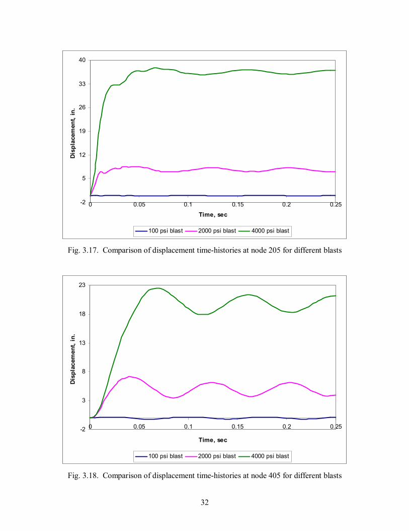
maximum deflection of 37.61 in. at node 205. Comparative time histories for each of the
three cases are shown in Figs 3.17 and 3.18. Fig. 3.19 shows a sample von Mises stress
distribution of the frame. This blast caused plastic deformation across the majority of the
blast side column and a substantial portion of the beam (Fig. 3.20). Also evident in this
figure is the deflection of the blast side column relative to the rest of the frame.

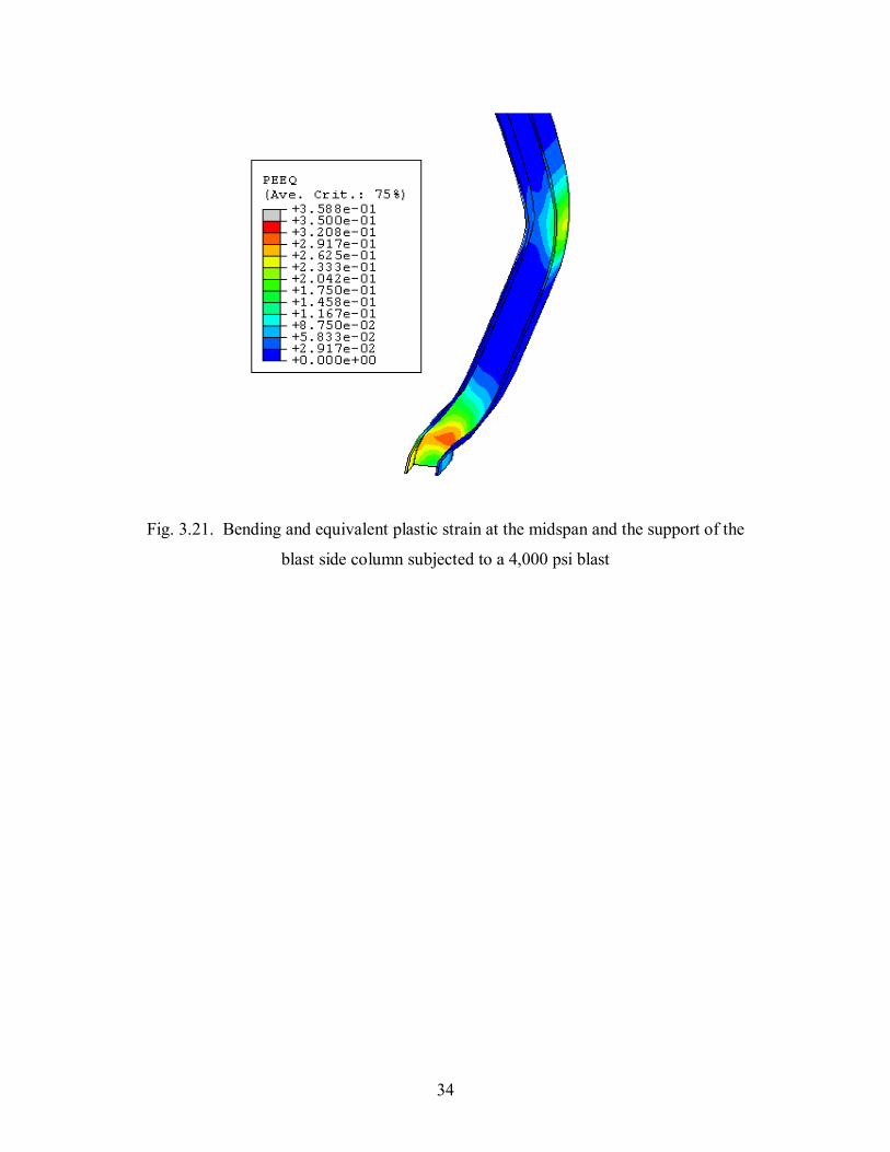
24
Significant bending can be seen at the midspan and in the flanges at the support (Fig.
3.22). The total time of the blast load was not long enough to force total failure of the
beam. Note the equivalent plastic strain in the member in the area. There is substantial
plastic strain in the web of the blast side column just above the support; however, these
values do not reach the failure strain of the material.

25
-0.4
-0.2
0
0.2
0.4
0 0.05 0.1 0.15 0.2 0.25
Time, sec
Dis
plac
emen
t, in
.
Fig. 3.4. Deflection time-history of node 405 for a 100 psi blast
-0.4
-0.2
0
0.2
0.4
0 0.05 0.1 0.15 0.2 0.25
Time, sec
Disp
lace
men
t, in
.
Fig. 3.5. Deflection time-history of node 11405 for a 100 psi blast

26
Fig. 3.6. Sample of von Mises stress distribution in the portal frame subjected to a 100
psi blast load
27
0
2
4
6
8
0 0.05 0.1 0.15 0.2 0.25
Time, sec
Disp
lace
men
t, in
.
Fig. 3.7. Deflection time-history of node 405 for a 2,000 psi blast
0
2
4
6
8
0 0.05 0.1 0.15 0.2 0.25
Time, sec
Disp
lace
men
t, in
.
Fig. 3.8. Deflection time-history of node 11405 for a 2,000 psi blast

28
0
2
4
6
8
10
0 0.05 0.1 0.15 0.2 0.25
Time, sec
Disp
lace
men
t, in
.
Fig. 3.9. Deflection time-history of node 205 for a 2,000 psi blast
0
2
4
6
8
10
0 0.05 0.1 0.15 0.2 0.25
Time, sec
Disp
lace
men
t, in
.
Fig. 3.10. Deflection time-history of node 11205 for a 2,000 psi blast
29
Fig. 3.11. Sample of von Mises stress distribution in the portal frame subjected to a
2,000 psi blast load at time t = 10 msec
Fig. 3.12. Plastic deformation zones of the portal frame subjected to a 2,000 psi blast (no
plastic deformation = blue) at time t = 0.25 sec

30
0
6
12
18
24
0 0.05 0.1 0.15 0.2 0.25
Time, sec
Disp
lace
men
t, in
.
Fig. 3.13. Deflection time-history of node 405 for a 4,000 psi blast
0
6
12
18
24
0 0.05 0.1 0.15 0.2 0.25
Time, sec
Disp
lace
men
t, in
.
Fig. 3.14. Deflection time-history of node 11405 for a 4,000 psi blast
31
0
8
16
24
32
40
0 0.05 0.1 0.15 0.2 0.25
Time, sec
Disp
lace
men
t, in
.
Fig. 3.15. Deflection time-history of node 205 for a 4,000 psi blast
0
5
10
15
0 0.05 0.1 0.15 0.2 0.25
Time, sec
Disp
lace
men
t, in
.
Fig. 3.16. Deflection time-history of node 11205 for a 4,000 psi blast
32
-2
5
12
19
26
33
40
0 0.05 0.1 0.15 0.2 0.25Time, sec
Disp
lace
men
t, in
.
100 psi blast 2000 psi blast 4000 psi blast
Fig. 3.17. Comparison of displacement time-histories at node 205 for different blasts
-2
3
8
13
18
23
0 0.05 0.1 0.15 0.2 0.25
Time, sec
Disp
lace
men
t, in
.
100 psi blast 2000 psi blast 4000 psi blast
Fig. 3.18. Comparison of displacement time-histories at node 405 for different blasts

33
Fig. 3.19. Sample of von Mises stress distribution in the portal frame subjected to a
4,000 psi blast load at time t = 20 msec
Fig. 3.20. Plastic deformation zones of the portal frame subjected to a 4,000 psi blast (no
plastic deformation = blue) at time t = 0.25 sec
34
Fig. 3.21. Bending and equivalent plastic strain at the midspan and the support of the
blast side column subjected to a 4,000 psi blast

35
Chapter 4
Effects of Bilinear Springs on the Models
4.1 SCEDs Modeled as Springs
Previous research by Pearson (2002) and Hennessey (2003) analyzed snapping-cable
energy dissipators (SCEDs) as possible passive earthquake dampers. The research done
to this point has focused on the properties of synthetic fiber ropes that are to be used as
SCEDs. The results of the work thus far have shown that these ropes behave similarly to
springs when in tension, but are not able to withstand any compressive force. This
research studies the use of these ropes as a means to resist the effects of blast loads.
Springs were introduced into the models by attaching them at the corners as an X-brace.
Figure 4.1 shows the ABAQUS model of the springs attached to the frame. The shape of
the springs is due to the fact that ABAQUS shapes the elements as coils. A more
accurate representation of how the ropes being modeled would actually be placed in the
frame can be seen in Fig. 4.2.
Fig. 4.1. ABAQUS representation of SCEDs introduced into the frame
36
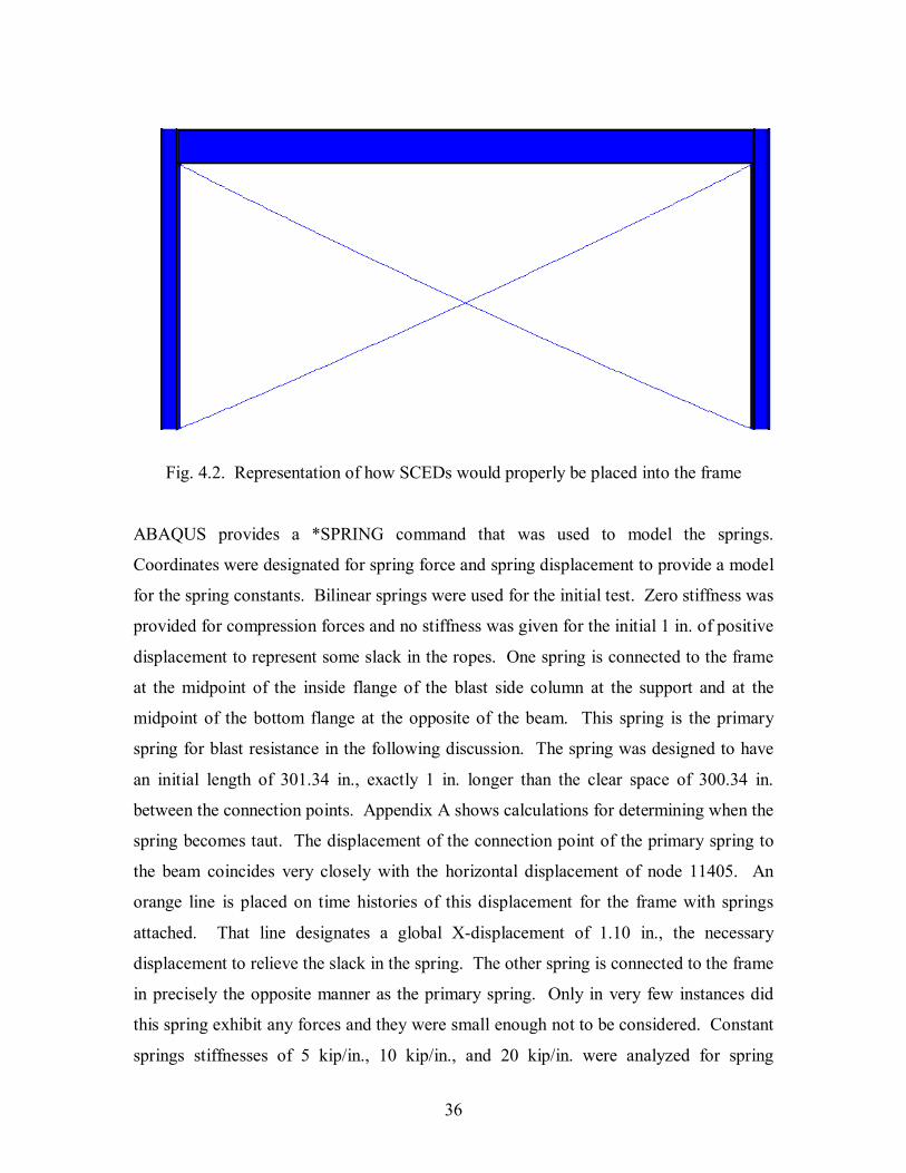
Fig. 4.2. Representation of how SCEDs would properly be placed into the frame
ABAQUS provides a *SPRING command that was used to model the springs.
Coordinates were designated for spring force and spring displacement to provide a model
for the spring constants. Bilinear springs were used for the initial test. Zero stiffness was
provided for compression forces and no stiffness was given for the initial 1 in. of positive
displacement to represent some slack in the ropes. One spring is connected to the frame
at the midpoint of the inside flange of the blast side column at the support and at the
midpoint of the bottom flange at the opposite of the beam. This spring is the primary
spring for blast resistance in the following discussion. The spring was designed to have
an initial length of 301.34 in., exactly 1 in. longer than the clear space of 300.34 in.
between the connection points. Appendix A shows calculations for determining when the
spring becomes taut. The displacement of the connection point of the primary spring to
the beam coincides very closely with the horizontal displacement of node 11405. An
orange line is placed on time histories of this displacement for the frame with springs
attached. That line designates a global X-displacement of 1.10 in., the necessary
displacement to relieve the slack in the spring. The other spring is connected to the frame
in precisely the opposite manner as the primary spring. Only in very few instances did
this spring exhibit any forces and they were small enough not to be considered. Constant
springs stiffnesses of 5 kip/in., 10 kip/in., and 20 kip/in. were analyzed for spring

37
displacements larger than 1 in. A graph of these spring forces is seen in Fig. 4.3. It
should also be noted that because of the initial 1 in. of zero stiffness, the frame subjected
to a 100 psi blast was not analyzed for the inclusion of the ropes. Under the given
parameters, the ropes did not become taut under a 100 psi blast; therefore, the frame did
not experience any spring forces.
0
200
400
600
800
0 10 20 30 40
Spring Displacement, in.
Sprin
g Fo
rce,
kip
5 kip/in. 10 kip/in. 20 kip/in.
Fig. 4.3. Graph of spring stiffnesses
4.2 Effects of Springs on Displacements
4.2.1 Case II – 2,000 psi blast
The effect of the springs on the displacements of the key nodes was beneficial, especially
at the connections. Figures 4.4, 4.5, 4.6, and 4.7 compare the displacement time histories
of nodes 205, 405, 11205, and 11405, respectively. The effect of the springs at node 205,
while noticeable, is much less substantial than the effect at nodes 405 and 11405. The
reduction in total deflection at node 205 is most likely attributed to the reductions at

38
nodes 405 and 11405. In terms of global deflection, there is a correlation between the
displacements at the midspan of a member relative to its end. The blast side column,
however, still experiences significant bending at midspan. The behavior of the frame at
nodes 405 and 11405 is positively affected by the springs. Table 4.1 shows a comparison
of the maximum displacement and the dynamic behavior of the frame at node 405 after
the blast load has ended. The time histories for nodes 405 and 11405 are nearly identical,
therefore a summarization of node 405 only will suffice. Tables 4.2 and 4.3 contain
similar data for nodes 205 and 11205 with the omission of period of vibration.
(kip/in.) (in.) (in.) (sec)No Springs 7.21 6.20 0.08
5 5.82 3.89 0.0710 5.25 2.91 0.06520 4.41 2.43 0.065
Spring StiffnessMaximum
DisplacementMaximum Displacement at Later Cycles of Motion
Period of Vibration
Table 4.1. Comparison of the structural behavior of the frame at node 405 with different
bracing spring stiffnesses subjected to a blast load of 2,000 psi
(kip/in.) (in.) (in.)No Springs 8.68 8.28
5 8.16 7.1010 7.75 6.6120 7.49 6.35
Spring StiffnessMaximum
DisplacementMaximum Displacement at Later Cycles of Motion
Table 4.2. Comparison of the structural behavior of the frame at node 205 with different
bracing spring stiffnesses subjected to a blast load of 2,000 psi
(kip/in.) (in.) (in.)No Springs 3.73 3.30
5 3.00 2.3010 2.72 1.8220 2.44 1.40
Spring StiffnessMaximum
DisplacementMaximum Displacement at Later Cycles of Motion
Table 4.3. Comparison of the structural behavior of the frame at node 11205 with
different bracing spring stiffnesses subjected to a blast load of 2,000 psi

39
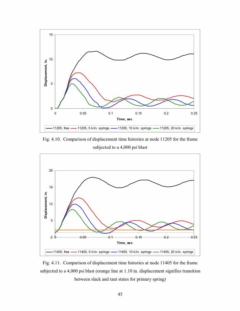
4.2.2 Case III – 4,000 psi blast
For case III, the springs had a much more significant effect. Figures 4.8, 4.9, 4.10, and
4.11 show the displacement time histories of the braced frame at each spring stiffness
subjected to a 4,000 psi blast. Section 3.2.3 described the large deflections that occurred
at the key nodes as a result of the 4,000 psi blast. The springs countered these large
deflections much more effectively than they countered the smaller deflections that were
caused by the 2,000 psi blast. Displacements were reduced by as much as 60% for the 20
kip/in. springs at nodes 405 and 11405. A large-scale reduction in the displacement of
node 205 is not evident. Table 4.4 shows a comparison of the maximum displacement
and the dynamic behavior of the frame at node 405 after the 4,000 blast load has ended.
Tables 4.5 and 4.6 contain similar data for nodes 205 and 11205. An important aspect of
the frame behavior with springs included is the high rate of reduction for the long-term
displacements of nodes 405 and 11405. The amplitude of displacement for the long-term
cycles of motion decreases by 80 percent, even for the 5 kip/in. spring.
(kip/in.) (in.) (in.) (sec)No Springs 22.43 21.36 0.09
5 13.3 4.4 0.08510 10.89 3.38 0.0820 8.67 3.62 0.075
Spring StiffnessMaximum
DisplacementMaximum Displacement at Later Cycles of Motion
Period of Vibration
Table 4.4. Comparison of the structural behavior of the frame at node 405 with different
bracing spring stiffnesses subjected to a blast load of 4,000 psi

40
(kip/in.) (in.) (in.)No Springs 37.61 37.15
5 34.35 29.1710 33.35 28.8420 32.49 29.27
Spring StiffnessMaximum
DisplacementMaximum Displacement at Later Cycles of Motion
Table 4.5. Comparison of the structural behavior of the frame at node 205 with different
bracing spring stiffnesses subjected to a blast load of 4,000 psi
(kip/in.) (in.) (in.)No Springs 11.63 11.23
5 7.3 2.7110 6.12 1.9720 4.99 2.26
Spring StiffnessMaximum
DisplacementMaximum Displacement at Later Cycles of Motion
Table 4.6. Comparison of the structural behavior of the frame at node 11205 with
different bracing spring stiffnesses subjected to a blast load of 4,000 psi
4.3 Effect of Springs on Plasticity Spread
Analysis of the models following the addition of springs showed that the presence of the
springs, even up to a spring stiffness of 20 kip/in., had no effect on the overall presence
of permanent plasticity in the frame. Figure 4.12 shows the plastic deformation zones for
the frame subjected to a 4,000 psi blast braced with 20 kip/in. springs. When compared
to Fig. 3.21, the plastic deformation zones are almost identical. As mentioned previously,
the overall plastic deformation of the frame was reduced, by as much as 50% in some
instances, by the presence of the springs. However, the spread of plasticity in the frame
concludes 3 msec into the model’s run. Further analysis of Figs. 4.4 – 4.11 shows that
the springs do not begin to aid in deflections until 2-3 msec into the analysis, after almost
all of the permanent plasticity has occurred.

41
Note in Fig. 4.13 that the displacement at node 11405 for a bare frame does not reach
1.10 in.—the boundary for tension in the spring—until just after time t = 5 msec. It was
previously noted that node 11405 will displace almost identically to the connection point
of the tension spring. Figure 4.14 shows the plasticity in the frame at time t = 5 msec.
When compared to Fig. 4.12, most of the plasticity spread in the blast side column has
already occurred. It is also noted that almost no rebound occurs following the 4,000 psi
blast, while a rebound between 10-15% takes place at nodes 405 and 11405 following the
2,000 psi blast.

42
-1
1
3
5
7
9
0 0.05 0.1 0.15 0.2 0.25
Time, sec
Disp
lace
men
t, in
.
205, free 205, 5 k/in. springs 205, 10 k/in. springs 205, 20 k/in. springs
Fig. 4.4. Comparison of displacement time histories at node 205 for the frame subjected
to a 2,000 psi blast
-1
1
3
5
7
9
0 0.05 0.1 0.15 0.2 0.25
Time, sec
Disp
lace
men
t, in
.
405, free 405, 5 k/in. springs 405, 10 k/in. springs 405, 20 k/in. springs
Fig. 4.5. Comparison of displacement time histories at node 405 for the frame subjected
to a 2,000 psi blast

43
-1
1
3
5
7
9
0 0.05 0.1 0.15 0.2 0.25
Time, sec
Disp
lace
men
t, in
.
11205, free 11205, 5 k/in. springs 11205, 10 k/in. springs 11205, 20 k/in. springs
Fig. 4.6. Comparison of displacement time histories at node 11205 for the frame
subjected to a 2,000 psi blast
-1
1
3
5
7
9
0 0.05 0.1 0.15 0.2 0.25
Time, sec
Disp
lace
men
t, in
.
11405, free 11405, 5 k/in. springs 11405, 10 k/in. springs 11405, 20 k/in. springs
Fig. 4.7. Comparison of displacement time histories at node 11405 for the frame
subjected to a 2,000 psi blast (orange line at 1.10 in. displacement signifies transition
between slack and taut states for primary spring)

44
-2
5
12
19
26
33
40
0 0.05 0.1 0.15 0.2 0.25
Time, sec
Disp
lace
men
t, in
.
205, free 205, 5 k/in. springs 205, 10 k/in. springs 205, 20 k/in. springs
Fig. 4.8. Comparison of displacement time histories at node 205 for the frame subjected
to a 4,000 psi blast
-2
5
12
19
26
0 0.05 0.1 0.15 0.2 0.25
Time, sec
Disp
lace
men
t, in
.
405, free 405, 5 k/in. springs 405, 10 k/in. springs 405, 20 k/in. springs
Fig. 4.9. Comparison of displacement time histories at node 405 for the frame subjected
to a 4,000 psi blast
45
0
5
10
15
0 0.05 0.1 0.15 0.2 0.25
Time, sec
Disp
lace
men
t, in
.
11205, free 11205, 5 k/in. springs 11205, 10 k/in. springs 11205, 20 k/in. springs
Fig. 4.10. Comparison of displacement time histories at node 11205 for the frame
subjected to a 4,000 psi blast
-2
5
12
19
26
0 0.05 0.1 0.15 0.2 0.25Time, sec
Disp
lace
men
t, in
.
11405, free 11405, 5 k/in. springs 11405, 10 k/in. springs 11405, 20 k/in. springs
Fig. 4.11. Comparison of displacement time histories at node 11405 for the frame
subjected to a 4,000 psi blast (orange line at 1.10 in. displacement signifies transition
between slack and taut states for primary spring)
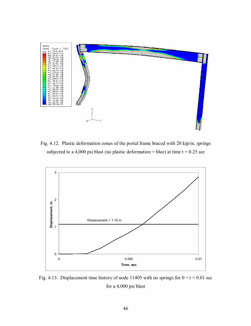
46
Fig. 4.12. Plastic deformation zones of the portal frame braced with 20 kip/in. springs
subjected to a 4,000 psi blast (no plastic deformation = blue) at time t = 0.25 sec
Displacement = 1.10 in.
0
1
2
3
0 0.005 0.01
Time, sec
Disp
lace
men
t, in
.
Fig. 4.13. Displacement time history of node 11405 with no springs for 0 < t < 0.01 sec
for a 4,000 psi blast

47
Fig. 4.14. Plastic deformation zones of the bare portal frame subjected to a 4,000 psi
blast (no plastic deformation = blue) at time t = 5 msec

48
Chapter 5
Inclusion of Strain Rate Effects
5.1 Strain Rate Effects
The loading on a structure resulting from a blast has been discussed in detail thus far.
The loads are much higher than most loads that a structure will experience, and occur
over a much shorter time period. When a large dynamic load such as a blast load causes
a material to begin to yield, it is common that the strain rate in the material will be higher
than usual. Williams and Newell (1991) explain that materials loaded at high strain rates
typically tend to exhibit higher yield strengths and greater ductilities than they would
generally exhibit under a static load. Changes in values such as the modulus of elasticity
and other material properties are negligible.
Shope and Plaut (1998) examined critical blast loads for compressed steel columns and
determined that the inclusion of strain rate dependent yielding in their analysis resulted in
an increase in critical blast impulse of approximately ten percent. Typically, when a
structure is subjected to a loading that produces uniformly high material strain rates, a
single dynamic increase factor is included. For the models analyzed by Shope and Plaut,
strain rate effects were introduced based on a material model given in NAVFAC (1990)
that is applicable for in-depth analyses with variations in dynamic increase factor (Eq.
5.1). A logarithmic increase is applied to the dynamic yield strength with an increase in
strain rate. A similar tabulated rate dependent model was used for this research by
inserting a *RATE DEPENDENT command into the material property section of the
ABAQUS input file. This model can be seen in Fig. 5.1.
Dynamic Increase Factor = y
dy
σσ
(5.1)
where σdy = dynamic yield stress;
σy = static yield stress.

49
1
1.2
1.4
1.6
1.8
2
0.001 0.01 0.1 1 10 100
Strain Rate, in./in./sec
Dyna
mic
Incr
ease
Fac
tor
Fig. 5.1. Dynamic yield strength of the frame material based on strain rate
The effects of high strain rates were analyzed for cases II and III—the 2,000 psi and
4,000 psi blasts, respectively. The results of these analyses and a comparison of models
with and without the inclusion of high strain rate effects can be found in sections 5.2-5.4.
It should be noted that the 10 kip/in. bilinear spring was omitted from these analyses
based on the results of the models from Chapter 4.
5.2 High Strain Rate Effects on Frame Displacements
5.2.1 Case II – 2,000 psi blast
Figures 5.2-5.13 compare displacement time histories for the frame subjected to a 2,000
psi blast with and without the inclusion of rate dependent yield effects. Figures 5.2-5.5
show the time histories of nodes 205, 405, 11205, and 11405, respectively with no
springs on the frame. Figures 5.6-5.9 display the time histories of nodes 205, 405, 11205,
and 11405, respectively, with 5 kip/in. springs bracing the frame. Figures 5.10-5.13
show the time histories of nodes 205, 405, 11205, and 11405, respectively, for the frame
braced with 20 kip/in. springs. Figures showing displacement time histories for node

50
11405 contain the orange line marking the point where the “slack” is removed from the
springs at 1.10 in. of displacement.
Initial analysis of these 12 figures shows that the higher strain rate effects clearly have a
significant impact on the behavior of the system. Including the rate dependent yield
effects increases the yield stress of the material, thereby decreasing the displacement of
the system. With no springs included, the deflection of node 405 is higher than that of
node 205, signifying a decrease in midspan bending in the blast side column.
Comparisons of Figs. 5.2-5.5 and Figs. 5.6-5.13 show that the inclusion of springs
diminishes the effects of higher strain rates, especially at nodes 405 and 11405. Figures
5.11-5.13 show that the 20 kip/in. spring nearly negates the effects of high strain rates at
these nodes. The higher strain rates have similar effects on node 205 regardless of
springs. The behavior of node 205 is based much more on the blast than on the total
structural system that is in place. The springs do not restrict the displacement at node
205.
Tables 5.1-5.3 examine the inclusion of rate dependent yield effects on the structure.
Note that strain rate effects have been designated SRE. Furthermore, note that the
behavior of node 11405 is almost identical to that of node 405; therefore, it has been
omitted from the tables.
Node 205 8.68 5.59 8.28 5.02Node 405 7.21 6.02 6.20 4.99
Node 11205 3.73 2.94 3.30 2.55
Maximum Displacement, No SRE (in.)
Maximum Displacement at
Later Cycles, No SRE (in.)
Maximum Displacement,
SRE (in.)
Maximum Displacement at
Later Cycles, SRE (in.)
Table 5.1. Effects of the inclusion of rate dependent yield on the bare frame subjected to
a 2,000 psi blast

51
Node 205 8.16 5.36 7.10 4.35Node 405 5.82 5.22 3.89 3.70
Node 11205 3.00 2.58 2.30 2.17
Maximum Displacement, No SRE (in.)
Maximum Displacement
at Later Cycles, No SRE (in.)
Maximum Displacement,
SRE (in.)
Maximum Displacement at
Later Cycles, SRE (in.)
Table 5.2. Effects of the inclusion of rate dependent yield on the frame braced with 5
kip/in. springs subjected to a 2,000 psi blast
Node 205 7.49 5.26 6.35 3.82Node 405 4.41 4.33 2.43 2.67
Node 11205 2.44 2.16 1.40 1.45
Maximum Displacement, No SRE (in.)
Maximum Displacement
at Later Cycles, No SRE (in.)
Maximum Displacement,
SRE (in.)
Maximum Displacement at
Later Cycles, SRE (in.)
Table 5.3. Effects of the inclusion of rate dependent yield on the frame braced with 20
kip/in. springs subjected to a 2,000 psi blast
5.2.2 Case III – 4,000 psi blast
Figures 5.14-5.25 compare displacement time histories for the frame subjected to a 4,000
psi blast with and without the inclusion of rate dependent yield effects, similar to those
described in section 5.2.1. Figures 5.14-5.17 show the time histories of nodes 205, 405,
11205, and 11405, respectively with no springs on the frame. Figures 5.18-5.21 display
the time histories of nodes 205, 405, 11205, and 11405, respectively, with 5 kip/in.
springs bracing the frame. Figures 5.22-5.25 show displacement time histories of nodes
205, 405, 11205, and 11405, respectively, for the frame braced with 20 kip/in. springs.
Figures that display displacement time histories for node 11405 contain the orange line
marking the point where the “slack” is removed from the springs at 1.10 in. of
displacement.
Investigation of these figures shows that the higher strain rate effects on the frame
subjected to a 4,000 psi blast have a similar impact on the behavior of the system as in

52
the case of a 2,000 psi blast. Comparisons of Figs. 5.14-5.17 and Figs. 5.18-5.25 show
that the inclusion of springs again diminishes the effects of higher strain rates. Tables
5.4-5.6 examine the inclusion of rate dependent yield effects on the structure.
Node 205 37.61 23.49 37.15 22.63Node 405 22.43 16.71 21.36 14.79
Node 11205 11.63 8.48 11.23 7.85
Maximum Displacement, No SRE (in.)
Maximum Displacement
at Later Cycles, No SRE (in.)
Maximum Displacement,
SRE (in.)
Maximum Displacement at
Later Cycles, SRE (in.)
Table 5.4. Effects of the inclusion of rate dependent yield on the bare frame subjected to
a 4,000 psi blast
Node 205 34.35 21.28 29.17 18.39Node 405 13.30 12.15 4.40 5.99
Node 11205 7.30 6.46 2.71 3.47
Maximum Displacement, No SRE (in.)
Maximum Displacement
at Later Cycles, No SRE (in.)
Maximum Displacement,
SRE (in.)
Maximum Displacement at
Later Cycles, SRE (in.)
Table 5.5. Effects of the inclusion of rate dependent yield on the frame braced with 5
kip/in. springs subjected to a 4,000 psi blast
Node 205 32.49 19.75 29.27 17.29Node 405 8.67 8.25 3.62 3.94
Node 11205 4.99 4.94 2.26 2.27
Maximum Displacement, No SRE (in.)
Maximum Displacement
at Later Cycles, No SRE (in.)
Maximum Displacement,
SRE (in.)
Maximum Displacement at
Later Cycles, SRE (in.)
Table 5.6. Effects of the inclusion of rate dependent yield on the frame braced with 20
kip/in. springs subjected to a 4,000 psi blast

53
0
2.5
5
7.5
10
0 0.05 0.1 0.15 0.2 0.25
Time, sec
Disp
lace
men
t, in
.
No Strain Rate Effects Strain Rate Effects
Fig. 5.2. Displacement time-histories with and without the inclusion of high strain rate
effects at node 205 for the frame subjected to a 2,000 psi blast with no springs
0
2
4
6
8
0 0.05 0.1 0.15 0.2 0.25
Time, sec
Disp
lace
men
t, in
.
No Strain Rate Effects Strain Rate Effects.
Fig. 5.3. Displacement time-histories with and without the inclusion of high strain rate
effects at node 405 for the frame subjected to a 2,000 psi blast with no springs

54
0
1
2
3
4
0 0.05 0.1 0.15 0.2 0.25
Time, sec
Disp
lace
men
t, in
.
No Strain Rate Effects Strain Rate Effects
Fig. 5.4. Displacement time-histories with and without the inclusion of high strain rate
effects at node 11205 for the frame subjected to a 2,000 psi blast with no springs
0
2
4
6
8
0 0.05 0.1 0.15 0.2 0.25
Time, sec
Disp
lace
men
t, in
.
No Strain Rate Effects Strain Rate Effects
Fig. 5.5. Displacement time-histories with and without the inclusion of high strain rate
effects at node 11405 for the frame subjected to a 2,000 psi blast with no springs

55
0
2.5
5
7.5
10
0 0.05 0.1 0.15 0.2 0.25
Time, sec
Disp
lace
men
t, in
.
No Strain Rate Effects Strain Rate Effects
Fig. 5.6. Displacement time-histories with and without the inclusion of high strain rate
effects at node 205 for the frame subjected to a 2,000 psi blast with 5 kip/in. bilinear
springs
0
2
4
6
8
0 0.05 0.1 0.15 0.2 0.25
Time, sec
Disp
lace
men
t, in
.
No Strain Rate Effects Strain Rate Effects
Fig. 5.7. Displacement time-histories with and without the inclusion of high strain rate
effects at node 405 for the frame subjected to a 2,000 psi blast with 5 kip/in. bilinear
springs

56
0
1
2
3
4
0 0.05 0.1 0.15 0.2 0.25
Time, sec
Disp
lace
men
t, in
.
No Strain Rate Effects Strain Rate Effects
Fig. 5.8. Displacement time-histories with and without the inclusion of high strain rate
effects at node 11205 for the frame subjected to a 2,000 psi blast with 5 kip/in. bilinear
springs
0
2
4
6
8
0 0.05 0.1 0.15 0.2 0.25
Time, sec
Disp
lace
men
t, in
.
No Strain Rate Effects Strain Rate Effects Boundary for Tension Spring Slack
Fig. 5.9. Displacement time-histories with and without the inclusion of high strain rate
effects at node 11405 for the frame subjected to a 2,000 psi blast with 5 kip/in. bilinear
springs

57
0
2
4
6
8
0 0.05 0.1 0.15 0.2 0.25
Time, sec
Disp
lace
men
t, in
.
No Strain Rate Effects Strain Rate Effects
Fig. 5.10. Displacement time-histories with and without the inclusion of high strain rate
effects at node 205 for the frame subjected to a 2,000 psi blast with 20 kip/in. bilinear
springs
-2
0
2
4
6
0 0.05 0.1 0.15 0.2 0.25
Time, sec
Disp
lace
men
t, in
.
No Strain Rate Effects Strain Rate Effects.
Fig. 5.11. Displacement time-histories with and without the inclusion of high strain rate
effects at node 405 for the frame subjected to a 2,000 psi blast with 20 kip/in. bilinear
springs

58
-1
0
1
2
3
0 0.05 0.1 0.15 0.2 0.25
Time, sec
Disp
lace
men
t, in
.
No Strain Rate Effects Strain Rate Effects
Fig. 5.12. Displacement time-histories with and without the inclusion of high strain rate
effects at node 11205 for the frame subjected to a 2,000 psi blast with 20 kip/in. bilinear
springs
-2
0
2
4
6
0 0.05 0.1 0.15 0.2 0.25
Time, sec
Dis
plac
emen
t, in
.
No Strain Rate Effects Strain Rate Effects Boundary for Tension Spring Slack
Fig. 5.13. Displacement time-histories with and without the inclusion of high strain rate
effects at node 11405 for the frame subjected to a 2,000 psi blast with 20 kip/in. bilinear
springs
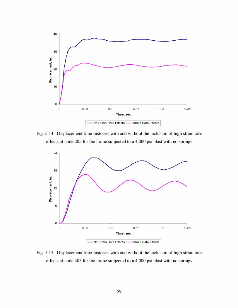
59
0
10
20
30
40
0 0.05 0.1 0.15 0.2 0.25
Time, sec
Disp
lace
men
t, in
.
No Strain Rate Effects Strain Rate Effects
Fig. 5.14. Displacement time-histories with and without the inclusion of high strain rate
effects at node 205 for the frame subjected to a 4,000 psi blast with no springs
0
6
12
18
24
0 0.05 0.1 0.15 0.2 0.25
Time, sec
Disp
lace
men
t, in
.
No Strain Rate Effects Strain Rate Effects
Fig. 5.15. Displacement time-histories with and without the inclusion of high strain rate
effects at node 405 for the frame subjected to a 4,000 psi blast with no springs

60
0
3
6
9
12
0 0.05 0.1 0.15 0.2 0.25
Time, sec
Disp
lace
men
t, in
.
No Strain Rate Effects Strain Rate Effects
Fig. 5.16. Displacement time-histories with and without the inclusion of high strain rate
effects at node 11205 for the frame subjected to a 4,000 psi blast with no springs
0
6
12
18
24
0 0.05 0.1 0.15 0.2 0.25
Time, sec
Disp
lace
men
t, in
.
No Strain Rate Effects Strain Rate Effects
Fig. 5.17. Displacement time-histories with and without the inclusion of high strain rate
effects at node 11405 for the frame subjected to a 4,000 psi blast with no springs

61
0
9
18
27
36
0 0.05 0.1 0.15 0.2 0.25
Time, sec
Disp
lace
men
t, in
.
No Strain Rate Effects Strain Rate Effects
Fig. 5.18. Displacement time-histories with and without the inclusion of high strain rate
effects at node 205 for the frame subjected to a 4,000 psi blast with 5 kip/in. bilinear
springs
0
4
8
12
16
0 0.05 0.1 0.15 0.2 0.25
Time, sec
Disp
lace
men
t, in
.
No Strain Rate Effects Strain Rate Effects
Fig. 5.19. Displacement time-histories with and without the inclusion of high strain rate
effects at node 405 for the frame subjected to a 4,000 psi blast with 5 kip/in. bilinear
springs

62
0
2
4
6
8
0 0.05 0.1 0.15 0.2 0.25
Time, sec
Disp
lace
men
t, in
.
No Strain Rate Effects Strain Rate Effects
Fig. 5.20. Displacement time-histories with and without the inclusion of high strain rate
effects at node 11205 for the frame subjected to a 4,000 psi blast with 5 kip/in. bilinear
springs
0
4
8
12
16
0 0.05 0.1 0.15 0.2 0.25
Time, sec
Disp
lace
men
t, in
.
No Strain Rate Effects Strain Rate Effects Boundary for Tension Spring Slack
Fig. 5.21. Displacement time-histories with and without the inclusion of high strain rate
effects at node 11405 for the frame subjected to a 4,000 psi blast with 5 kip/in. bilinear
springs

63
0
9
18
27
36
0 0.05 0.1 0.15 0.2 0.25
Time, sec
Disp
lace
men
t, in
.
No Strain Rate Effects Strain Rate Effects
Fig. 5.22. Displacement time-histories with and without the inclusion of high strain rate
effects at node 205 for the frame subjected to a 4,000 psi blast with 20 kip/in. bilinear
springs
-2
1
4
7
10
0 0.05 0.1 0.15 0.2 0.25
Time, sec
Dis
plac
emen
t, in
.
No Strain Rate Effects Strain Rate Effects
Fig. 5.23. Displacement time-histories with and without the inclusion of high strain rate
effects at node 405 for the frame subjected to a 4,000 psi blast with 20 kip/in. bilinear
springs

64
-1
1
3
5
7
0 0.05 0.1 0.15 0.2 0.25
Time, sec
Dis
plac
emen
t, in
.
No Strain Rate Effects Strain Rate Effects
Fig. 5.24. Displacement time-histories with and without the inclusion of high strain rate
effects at node 11205 for the frame subjected to a 4,000 psi blast with 20 kip/in. bilinear
springs
-2
1
4
7
10
0 0.05 0.1 0.15 0.2 0.25
Time, sec
Dis
plac
emen
t, in
.
No Strain Rate Effects Strain Rate Effects Boundary for Tension Spring Slack
Fig. 5.25. Displacement time-histories with and without the inclusion of high strain rate
effects at node 11405 for the frame subjected to a 4,000 psi blast with 20 kip/in. bilinear
springs

65
5.3 High Strain Rate Effects on Material Stresses
An elastic-perfectly plastic constitutive material relationship with a material yield stress
of 50 ksi was used for these analyses. Because of the bilinear nature of such a material
relationship, the stresses in the models do not exceed the yield stress throughout the
duration of the analysis, regardless of plastic strain. This is evident in Figs. 3.12 and
3.20. The inclusion of rate dependent yield in the models increases the material yield
stress by a dynamic increase factor relative to the strain rate (Fig. 5.1). The material
behavior beyond the yield point, however, remains constant the same way it would with a
dynamic increase factor of 1.0. This relationship is shown in Fig. 5.26.
Fig. 5.26. Stress-strain relationship with and without a dynamic increase factor
Based on these properties, stresses in the frame reached values much higher than 50 ksi,
depending upon the strain rate. Sample images of the von Mises stresses in a bare frame
with 2,000 psi and 4,000 psi blast loadings are shown in Figs. 5.27 and 5.28, respectively.
Noting the scale on the left hand side of the figures, stresses are as high as 84 ksi,
corresponding to a dynamic increase factor of 1.68 and a strain rate of about 30 in./in./sec
(see Fig. 5.1). The inclusion of springs again had little effect on the stresses in the frame
(Fig. 5.29). This was discussed in Chapter 4.
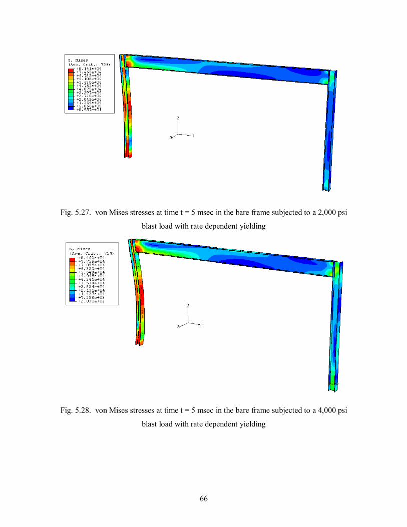
66
Fig. 5.27. von Mises stresses at time t = 5 msec in the bare frame subjected to a 2,000 psi
blast load with rate dependent yielding
Fig. 5.28. von Mises stresses at time t = 5 msec in the bare frame subjected to a 4,000 psi
blast load with rate dependent yielding

67
Fig. 5.29. von Mises stresses at time t = 5 msec in the frame braced with 20 kip/in.
springs subjected to a 4,000 psi blast load with rate dependent yielding

68
5.4 High Strain Rate Effects on Material Plasticity
The spread of plasticity in the frame was again unaffected by the introduction of springs
into the model. Figures 5.30 and 5.31 show the plastic deformation zones in the frame
subjected to a 2,000 psi blast without springs and with 20 kip/in. springs, respectively.
Figures 5.32 and 5.33 show similar models subjected to a 4,000 psi blast. Note that the
stresses are nearly identical with and without springs.
The rate dependent yield effects, however, did produce lower levels of permanent plastic
deformation in the frames. Comparisons of Figs. 5.30, 5.32, and 5.33 to Figs. 3.12, 3.20,
and 4.12, respectively, show that there is a considerable decrease in the percentage of the
frame that experiences permanent equivalent plastic strain. Figure 5.34 shows the
equivalent plastic strain in the lower half of the blast side column. The model shows a
maximum of 0.23 in./in. of strain, compared to a maximum value of 0.31 in./in. of strain
seen in Fig. 3.21. This coincides with the information in section 5.2 regarding the
reduced displacement resulting from the inclusion of rate dependent yield effects.

69
Fig. 5.30. Plastic deformation zones of the bare portal frame subjected to a 2,000 psi
blast (no plastic deformation = blue) at time t = 0.25 sec
Fig. 5.31. Plastic deformation zones of the portal frame braced with 20 kip/in. springs
subjected to a 2,000 psi blast (no plastic deformation = blue) at time t = 0.25 sec

70
Fig. 5.32. Plastic deformation zones of the bare portal frame subjected to a 4,000 psi
blast (no plastic deformation = blue) at time t = 0.25 sec
Fig. 5.33. Plastic deformation zones of the portal frame braced with 20 kip/in. springs
subjected to a 4,000 psi blast (no plastic deformation = blue) at time t = 0.25 sec

71
Fig. 5.34. Bending and equivalent plastic strain at the midspan and the support of the
blast side column subjected to a 4,000 psi blast, with high strain rate effects included

72
Chapter 6
Nonlinear Springs
6.1 Nonlinear Spring Properties
This research has examined the blast resistant effects of bilinear springs on portal frames.
Parallel research has been conducted regarding the material properties of the synthetic
ropes used as snapping cable energy dissipators (SCEDs) that the springs are modeling.
Initial tests of these ropes have suggested that the true force in the spring can be
approximated via the following equation:
3.1kxF = (6.1)
where k = spring stiffness (kip/(in.1.3))
x = axial displacement of the spring after the spring becomes taut
Spring models were created for this research using Eq. 6.1 and compared to the bilinear
results. Because the stiffnesses cannot directly coincide, several models were analyzed.
The bilinear spring stiffnesses of 5 kip/in. and 20 kip/in. were evaluated and, through trial
and error, spring stiffnesses in kip/(in.1.3) units were developed for comparisons. Two
means of comparison were developed—one where the bilinear spring stiffness was more
of an average of the nonlinear stiffness and another where the bilinear spring stiffness
was nearly tangent to the nonlinear stiffness at low displacements and never exceeds the
value of the nonlinear stiffness. Figures 6.1 and 6.2 show these comparisons.
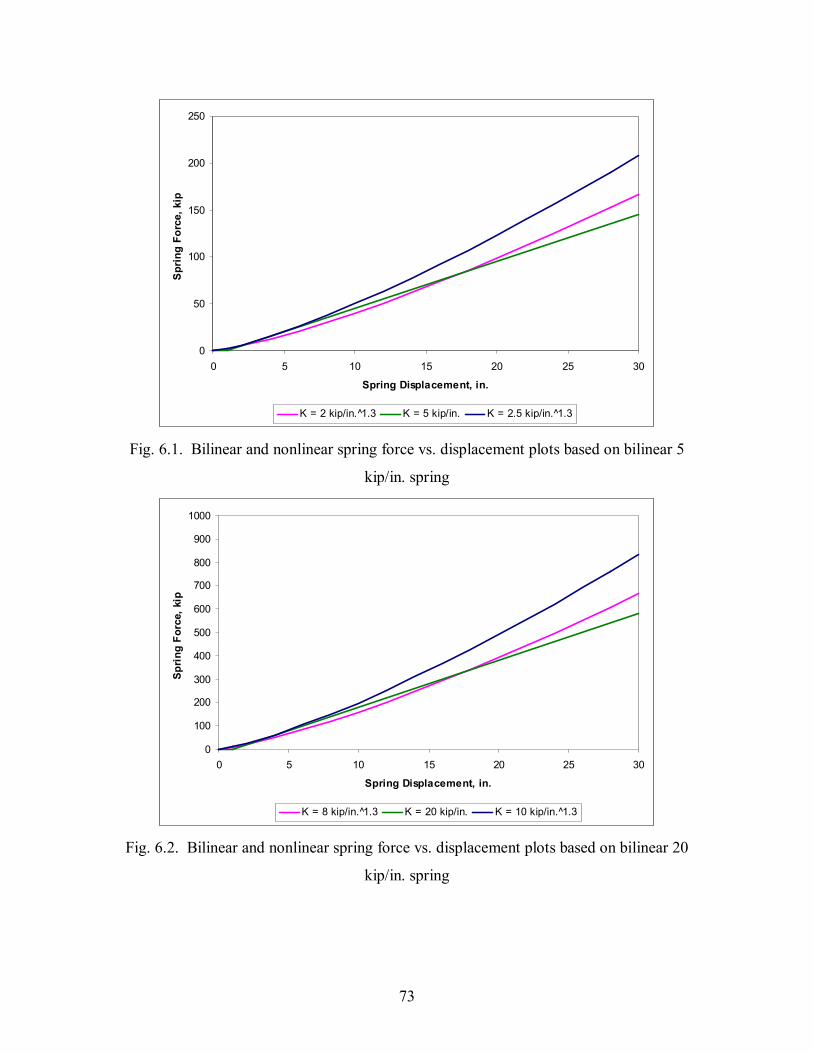
73
0
50
100
150
200
250
0 5 10 15 20 25 30
Spring Displacement, in.
Sprin
g Fo
rce,
kip
K = 2 kip/in. 1̂.3 K = 5 kip/in. K = 2.5 kip/in.^1.3
Fig. 6.1. Bilinear and nonlinear spring force vs. displacement plots based on bilinear 5
kip/in. spring
0
100
200
300
400
500
600
700
800
900
1000
0 5 10 15 20 25 30
Spring Displacement, in.
Sprin
g Fo
rce,
kip
K = 8 kip/in. 1̂.3 K = 20 kip/in. K = 10 kip/in.^1.3
Fig. 6.2. Bilinear and nonlinear spring force vs. displacement plots based on bilinear 20
kip/in. spring

74
It should be noted that the goal of this chapter was to compare effects of springs with
bilinear stiffnesses (bilinear springs) and nonlinear stiffnesses (nonlinear springs) on the
behavior of the frame system. This was done by ensuring that the nonlinear spring
stiffnesses were as close as possible to the bilinear spring stiffnesses. It was noted in
chapters 4 and 5 that the spring stiffnesses had little effect on the plasticity spread and the
stresses in the system. Analysis of the nonlinear springs showed that the stresses in the
system and the plasticity spread were nearly identical for the comparisons, as would be
expected. It should also be noted that rate dependent yield effects were considered in the
following analysis. The high strain rates caused by blast loads necessitate such
consideration for a more realistic analysis.
6.2 Displacement Comparisons
The subsections that follow detail the comparisons between bilinear and nonlinear
springs. The research discussed in the previous sections compared the structural behavior
of the frame subjected to varying blast loads, specifically 100 psi, 2,000 psi, and 4,000
psi blasts. For the purpose of comparing the bilinear and nonlinear springs, the 4,000 psi
blast was considered based on the higher displacements and more spring activity. These
higher spring forces make for a better means of comparison. Comparisons of the time
histories of the bilinear and nonlinear spring forces can be found in Appendix C.
6.2.1 Spring Case I – 5 kip/in. bilinear springs and corresponding nonlinear springs
The first step for comparing the bilinear and nonlinear springs was selecting the proper
nonlinear spring constants. Figure 6.1 shows a spring force vs. displacement diagram for
the 5 kip/in. bilinear spring. Nonlinear spring constants of 2 kip/in.1.3 and 2.5 kip/in.1.3
were selected for comparisons. The 2 kip/in.1.3 nonlinear spring has a lower spring
stiffness up to an axial displacement of 17.4 in., while the 2.5 kip/in.1.3 nonlinear spring
has a greater spring stiffness than the 5 kip/in. bilinear spring for all displacements. The

75
2.5 kip/in.1.3 nonlinear spring is nearly tangent to the 5 kip/in. bilinear spring at a
displacement of just under 4 in.
Figures 6.3-6.6 show displacement time histories at nodes 205, 405, 11205, and 11405,
respectively. These figures compare the system displacements for frames subjected to
4,000 psi blasts with each of the three different springs included. It is easily noted that
there is very little difference between the time histories for each of the three spring
stiffnesses, bilinear or nonlinear. The 2 kip/in.1.3 spring had slightly less effect on the
frame than the 5 kip/in. bilinear spring, while the 2.5 kip/in.1.3 showed slightly more
effect on the frame. This behavior would be expected since displacements do not exceed
17 in. at the nodes except in the case of node 205, which, as previously discussed, is least
affected by the springs. Table 6.1 compares maximum displacements for the key nodes
of the frame with different spring stiffnesses. Table 6.2 evaluates maximum
displacements at later cycles.
5 kip/in. bilinear spring
2 kip/in.1.3
nonlinear spring2.5 kip/in.1.3
nonlinear springNode 205 21.39 21.37 21.14Node 405 12.19 12.42 11.89
Node 11205 6.49 6.66 6.29Node 11405 12.88 13.11 12.57
Table 6.1. Maximum displacements at key nodes in the frame subjected to a 4,000 psi
blast and braced with springs with noted stiffnesses (base unit = inch)
5 kip/in. bilinear spring
2 kip/in.1.3
nonlinear spring2.5 kip/in.1.3
nonlinear springNode 205 18.42 18.86 18.45Node 405 5.91 6.98 6.18
Node 11205 3.45 3.90 3.36Node 11405 6.33 7.70 6.73
Table 6.2. Maximum displacements at later cycles at key nodes in the frame subjected to
a 4,000 psi blast and braced with springs with noted stiffnesses (base unit = inch)

76
6.2.2 Spring Case II – 20 kip/in. bilinear springs and corresponding nonlinear springs
Figure 6.2 shows a spring force vs. displacement diagram for the 20 kip/in. bilinear
spring. Based on the fact that the 20 kip/in. bilinear spring is 4 times stiffer than the 5
kip/in. bilinear spring, corresponding nonlinear spring constants of 8 kip/in.1.3 and 10
kip/in.1.3 were selected for comparisons. Similarly, the 8 kip/in.1.3 nonlinear spring has a
lower spring stiffness up to an axial displacement near 17.4 in., while the 10 kip/in.1.3
nonlinear spring has a higher spring stiffness than the 20 kip/in. bilinear spring for all
displacements. The 10 kip/in.1.3 nonlinear spring is nearly tangent to the 20 kip/in.
bilinear spring at a displacement of just under 4 in.
Figures 6.7-6.10 show displacement time histories at nodes 205, 405, 11205, and 11405,
respectively, comparing the system displacements for frames subjected to the same 4,000
psi blasts with each of the three different springs included. Note that there is again very
little difference between the time histories for each of the three spring stiffnesses, bilinear
or nonlinear. The difference for this set of comparisons is less than for the comparisons
made in the previous subsection. The 8 kip/in.1.3 spring had slightly less effect on the
frame than the 20 kip/in. bilinear spring, while the 10 kip/in.1.3 spring had slightly more
effect on the frame. Table 6.3 compares maximum displacements for the key nodes of
the frame with different spring stiffnesses. Table 6.4 shows maximum displacements at
later cycles of motion.
20 kip/in. bilinear spring
8 kip/in.1.3
nonlinear spring10 kip/in.1.3
nonlinear springNode 205 19.86 20.00 19.66Node 405 8.26 8.52 8.03
Node 11205 4.95 5.08 4.83Node 11405 9.06 9.27 8.81
Table 6.3. Maximum displacements at key nodes in the frame subjected to a 4,000 psi
blast and braced with springs with noted stiffnesses (base unit = inch)

77
20 kip/in. bilinear spring
8 kip/in.1.3
nonlinear spring10 kip/in.1.3
nonlinear springNode 205 17.43 17.41 17.24Node 405 4.13 4.07 3.78
Node 11205 2.32 2.23 2.11Node 11405 4.82 4.57 4.38
Table 6.4. Maximum displacements at later cycles at key nodes in the frame subjected to
a 4,000 psi blast and braced with springs with noted stiffnesses (base unit = inch)

78
0
9
18
27
36
0 0.03 0.06 0.09 0.12 0.15
Time, sec
Disp
lace
men
t, in
.
2 kip/in.^1.3 nonlinear spring 5 kip/in. bilinear spring 2.5 kip/in.^1.3 nonlinear spring
Fig. 6.3. Displacement time-histories for 5 kip/in. bilinear springs and corresponding
nonlinear springs for node 205 of the frame subjected to a 4,000 psi blast
0
4
8
12
16
20
0 0.03 0.06 0.09 0.12 0.15
Time, sec
Disp
lace
men
t, in
.
2 kip/in. 1̂.3 nonlinear spring 5 kip/in. bilinear spring 2.5 kip/in. 1̂.3 nonlinear spring
Fig. 6.4. Displacement time-histories for 5 kip/in. bilinear springs and corresponding
nonlinear springs for node 405 of the frame subjected to a 4,000 psi blast

79
0
2
4
6
8
0 0.03 0.06 0.09 0.12 0.15
Time, sec
Disp
lace
men
t, in
.
2 kip/in. 1̂.3 nonlinear spring 5 kip/in. bilinear spring 2.5 kip/in. 1̂.3 nonlinear spring
Fig. 6.5. Displacement time-histories for 5 kip/in. bilinear springs and corresponding
nonlinear springs for node 11205 of the frame subjected to a 4,000 psi blast
0
4
8
12
16
20
0 0.03 0.06 0.09 0.12 0.15
Time, sec
Disp
lace
men
t, in
.
2 kip/in.^1.3 nonlinear spring 5 kip/in. bilinear spring 2.5 kip/in.^1.3 nonlinear spring
Fig. 6.6. Displacement time-histories for 5 kip/in. bilinear springs and corresponding
nonlinear springs for node 11405 of the frame subjected to a 4,000 psi blast

80
0
9
18
27
36
0 0.03 0.06 0.09 0.12 0.15
Time, sec
Disp
lace
men
t, in
.
8 kip/in. 1̂.3 nonlinear spring 20 kip/in. bilinear spring 10 kip/in. 1̂.3 nonlinear spring
Fig. 6.7. Displacement time-histories for 20 kip/in. bilinear springs and corresponding
nonlinear springs for node 205 of the frame subjected to a 4,000 psi blast
-4
0
4
8
12
16
20
0 0.03 0.06 0.09 0.12 0.15
Time, sec
Disp
lace
men
t, in
.
8 kip/in. 1̂.3 nonlinear spring 20 kip/in. bilinear spring 10 kip/in. 1̂.3 nonlinear spring
Fig. 6.8. Displacement time-histories for 20 kip/in. bilinear springs and corresponding
nonlinear springs for node 405 of the frame subjected to a 4,000 psi blast
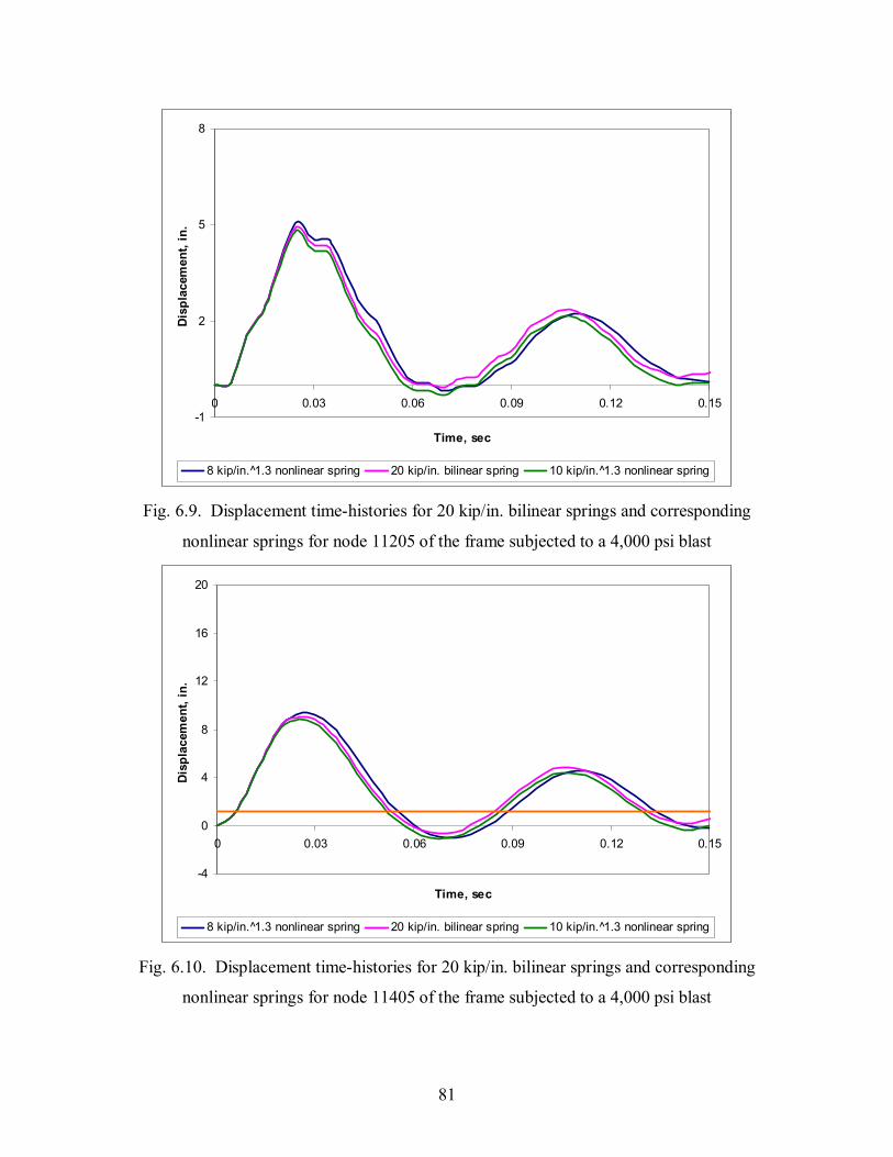
81
-1
2
5
8
0 0.03 0.06 0.09 0.12 0.15
Time, sec
Disp
lace
men
t, in
.
8 kip/in. 1̂.3 nonlinear spring 20 kip/in. bilinear spring 10 kip/in. 1̂.3 nonlinear spring
Fig. 6.9. Displacement time-histories for 20 kip/in. bilinear springs and corresponding
nonlinear springs for node 11205 of the frame subjected to a 4,000 psi blast
-4
0
4
8
12
16
20
0 0.03 0.06 0.09 0.12 0.15
Time, sec
Disp
lace
men
t, in
.
8 kip/in. 1̂.3 nonlinear spring 20 kip/in. bilinear spring 10 kip/in. 1̂.3 nonlinear spring
Fig. 6.10. Displacement time-histories for 20 kip/in. bilinear springs and corresponding
nonlinear springs for node 11405 of the frame subjected to a 4,000 psi blast

82
Chapter 7
Conclusions and Recommendations for Future Research
7.1 Summary and Conclusions
This research examined blast loads on portal frames and focused on methods of reducing
the effects of these loads. When an explosive device is detonated, a high-speed pressure
wave is created that can produce very high loads on a structure over very short time
spans. Many structures are not properly designed to resist these high loads; therefore,
research is underway to develop new methods of alleviating the effects of these loads.
This research is part of a multi-stage research project examining synthetic fiber ropes as a
means of lateral load resistance against seismic, blast, and wind loads. The long-term
goal of the project is to develop these ropes as Snapping-Cable Energy Dissipators
(SCEDs) that can be used as a structural element in a lateral load-resisting system.
The initial stages of this research project focused on the dynamic and material behavior
of the synthetic fiber ropes. Pearson (2002) and Hennessey (2003) studied these ropes
through experimental tests and analytical models. Their research is currently being
continued to better understand the exact behavior of the ropes. As the data from the
ropes are collected, alternate models are being developed to analyze the possible effects
of the ropes in structural systems. This thesis studied the effects of the ropes as blast
resistant structural elements through finite element analysis of blast loads on portal
frames. The commercial finite element program ABAQUS was used in all of the finite
element modeling, and both static and dynamic verification exercises were developed to
ensure the results of the models.
The frame models were created using 7,200 three-dimensional brick elements forming a
portal frame consisting of three steel I-beams with fixed supports and rigid connections.
An ideal unit blast curve was developed based on the Friedlander equation (Eq. 1.1) with
a maximum amplitude that can be modified in the ABAQUS input file to create varying

83
blast loads on the structure. The behavior of the frame subject to blast loads of 100,
2,000, and 4,000 psi was analyzed and key points of response were determined to exist at
the midspan and the top of each column. These key points were defined in Table 3.2 as
nodes 205, 405, 11205, and 11405. Time histories of displacements at the key nodes
were shown for each structural system that was analyzed as the primary form of
comparison. Initial tests of the blasts on the frame provided several important results.
First, the 100 psi blast proved to have very little effect overall on the structure, with
maximum displacements of about 0.2 in. at the corners of the frame. The 2,000 and
4,000 psi blasts showed substantial permanent displacement at each of the key points of
the structure, as high as 37 in. at the midspan of the blast side column. Equivalent plastic
strains in the web of the blast side column neared the point of failure. These are the
effects that the synthetic ropes are meant to resist.
The ropes were introduced into the model by developing bilinear springs as cross braces.
Physical models of the ropes in the frame would inherently have a small amount of slack
in the ropes. This was modeled by providing the spring zero stiffness to a displacement
of 1.0 in. Appendix A shows calculations to determine the necessary global X-
displacement for the transition between the slack and taut states in the ropes. Because of
the necessary displacement of 1.10 in. at node 11405, the 100 psi blast was not modeled
with springs. The first braced frame models were developed using bilinear springs with
stiffnesses of 5, 10, and 20 kip/in. The springs were shown to have a positive effect on
the displacement of the system at each of the key points of the frame. The effects of the
springs were more evident at nodes 405 and 11405—the tops of the columns—based on
the fact that the springs were connected to the frame at those points and had a more direct
effect there. Furthermore, the springs had much more effect on the system for the 4,000
psi blast than the 2,000 psi blast, most likely because the higher blast resulted in higher
displacements in the system. The springs were also shown to reduce the permanent
deformation at the key nodes by as much as 80% in some instances. The springs did not
have much effect on the maximum stresses and permanent plasticity in the system. Most
of the plasticity spread in the frame occurred before the springs became taut. However,
the level of equivalent plastic strain was positively affected by the stronger springs.

84
Blasts produce very large loads over short time periods; therefore, they result in high
strain rates. Because the structure cannot yield at the same rate as the load is applied, rate
dependent yield affects the behavior of the structure and a dynamic increase factor can be
applied to the yield stress of the material. This dynamic increase factor increases
logarithmically with the increase in strain rate (see Fig. 5.1). The dynamic increase
factor was proven to be integral for this research. Significant reductions in displacement
occurred following the introduction of rate dependent yield effects into the unbraced
system, specifically at the midspans of the columns relative to the tops of the columns.
However, the analysis showed that the inclusion of springs in the models reduced the
effects of high strain rates at nodes 405 and 11405. The 20 kip/in. bilinear spring nearly
negated the effects of rate dependent yield. Stresses in the material reached 84 ksi,
corresponding to a dynamic increase factor of 1.68 and a strain rate near 30 in./in./sec.
The corresponding critical strain points in the web of the base of the blast side column
showed significant reduction of strain of nearly 30%.
Parallel research showed that the spring forces based on displacement resulted in
nonlinear stiffnesses of kip/(in.1.3) instead of the bilinear stiffness in kip/in. Nonlinear
spring stiffnesses were used for comparison with the bilinear springs. Two nonlinear
models were developed for each bilinear model—one where the bilinear stiffness was
more of a trend line for the nonlinear stiffness and another where the bilinear stiffness
was nearly a tangent for the nonlinear stiffness (see Figs. 6.1 and 6.2). The data showed
that the behavior of the frame braced with nonlinear springs coincided very closely with
the behavior of the frame braced with bilinear springs.
The results of this research are promising. The springs that were modeled had a
definitively positive impact on the behavior of the frame. Large displacements lead to
failures that can be both costly and dangerous. Reducing these displacements is crucial
in the protection of the structure from blasts. The models provided in this research can be
valuable tools for determining the effects of the synthetic fiber ropes on the behavior of a
structure. The bilinear spring models were shown to closely coincide with the initial

85
models of the actual nonlinear behavior of the springs. For the models where the bilinear
spring stiffness was tangent to the nonlinear spring stiffness, the bilinear spring models
gave a slightly conservative method of accurately determining the behavior of the system.
7.2 Recommendations for Future Research
As previously mentioned, this is the third stage of a multi-stage research project. The
possibility of SCEDs as a means of lateral load resistance brings about the potential for
an adequate method of blast resistance that would be more cost-effective than designing
laterally braced structural systems or retrofitting existing buildings. To sufficiently
understand the effects that synthetic fiber ropes could have on structures, several steps
must be taken in future stages of this research.
First and foremost, the exact behavior of the ropes must be determined. Parallel research
is underway in developing the material properties of the ropes and their dynamic
behavior. The models developed for this research can easily be adapted for future
research by changing the commands within the ABAQUS input file. The models that
were analyzed in this research show that springs can be effective for reducing blast
response.
Second, to be able to apply these ropes to more realistic structural systems, large-scale
finite element modeling is recommended. Increasing the number of bays and creating a
three-dimensional model is feasible for the next level of this research. Models could also
be developed with various locations of the springs, alternative to X-bracing, to find the
system that most effectively mitigates the blast loads and reduces their effects.
The most beneficial research would be physical tests that could be run with scale models
of the frames. Currently scale model tests are being conducted to determine the behavior
of the synthetic ropes during seismic activity. Developing physical tests to analyze blast
loads is not a practical undertaking; however, the data that could be retrieved from these
tests would be invaluable to determining the nature of the rope behavior under such high

86
loads. Finally, additional uses of the SCEDs should be considered. More parallel
research is currently being developed for possible uses of the synthetic ropes for
mitigating bridge deflections and stabilizing towers. These types of applications could
lead to further use of SCEDs as a cost-effective means of bracing a structural system.
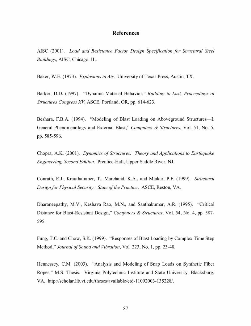
87
References
AISC (2001). Load and Resistance Factor Design Specification for Structural Steel
Buildings, AISC, Chicago, IL.
Baker, W.E. (1973). Explosions in Air. University of Texas Press, Austin, TX.
Barker, D.D. (1997). “Dynamic Material Behavior,” Building to Last, Proceedings of
Structures Congress XV, ASCE, Portland, OR, pp. 614-623.
Beshara, F.B.A. (1994). “Modeling of Blast Loading on Aboveground Structures—I.
General Phenomenology and External Blast,” Computers & Structures, Vol. 51, No. 5,
pp. 585-596.
Chopra, A.K. (2001). Dynamics of Structures: Theory and Applications to Earthquake
Engineering, Second Edition. Prentice-Hall, Upper Saddle River, NJ.
Conrath, E.J., Krauthammer, T., Marchand, K.A., and Mlakar, P.F. (1999). Structural
Design for Physical Security: State of the Practice. ASCE, Reston, VA.
Dharaneepathy, M.V., Keshava Rao, M.N., and Santhakumar, A.R. (1995). “Critical
Distance for Blast-Resistant Design,” Computers & Structures, Vol. 54, No. 4, pp. 587-
595.
Fung, T.C. and Chow, S.K. (1999). “Responses of Blast Loading by Complex Time Step
Method,” Journal of Sound and Vibration, Vol. 223, No. 1, pp. 23-48.
Hennessey, C.M. (2003). “Analysis and Modeling of Snap Loads on Synthetic Fiber
Ropes,” M.S. Thesis. Virginia Polytechnic Institute and State University, Blacksburg,
VA. http://scholar.lib.vt.edu/theses/available/etd-11092003-135228/.

88
Krauthammer, T. (1999). “Blast-resistant Structural Concrete and Steel Connections,”
International Journal of Impact Engineering, Vol. 22, No. 9-10, pp. 887-910.
Longinow, A. and Mniszewski, K.R. (1996). “Protecting Buildings Against Vehicle
Bomb Attacks,” Practice Periodical on Structural Design and Construction, Vol. 1, No.
1, pp. 51-54.
Miyamoto, H.K. and Taylor, D. (2000). “Structural Control of Dynamic Blast Loading,”
Advanced Technology in Structural Engineering, Proceedings from Structures Congress
2000, ASCE, Reston, VA, CD-ROM.
Mlakar, P.F. (1996). “Structural Design for Vehicular Bombs,” Building an International
Community of Structural Engineers, Vol. 2, pp. 1269-1276.
NAVFAC (1990). Structures to Resist the Effects of Accidental Explosions, Revision 1.
Dept. of the Navy Publication NAVFAC P-397, Dept. of the Army Technical Manual
TM-1300, Dept. of the Air Force Manual AFM 88-22, U.S. Depts. Of the Army, Navy,
and Air Force, Washington, DC.
Pearson, N.J. (2002). “Experimental Snap Loading of Synthetic Fiber Ropes,” M.S.
Thesis. Virginia Polytechnic Institute and State University, Blacksburg, VA.
http://scholar.lib.vt.edu/theses/available/etd-01132003-105300/.
Shope, R.L. and Plaut, R.H. (1998). “Critical Blast Loads for Compressed Steel
Columns,” Engineering Mechanics: A Force for the 21st Century, H. Murakami and J.E.
Luco, eds., ASCE, Reston, VA, pp. 712-715
Shope, R.L. and Plaut, R.H. (1999). “Critical Blast Loads for Two-Span Compressed
Steel Columns, Proceedings of the 13th Engineering Mechanics Division Conference,
N.P. Jones and R.G. Ghanem, eds.

89
Williams, M.S. and Newell, J.P. (1991). “Methods for the Assessment of the Blast
Response of Engineering Structures,” Earthquake, Blast, and Impact: Measurement and
Effects of Vibration, Society for Earthquake and Civil Engineering Design, E & F N
Spon, London, pp. 176-185.

90
Appendix A
Calculation of the Necessary Frame Displacement for Transformation
of the Springs from Slack to Taut State

91
A.1 Calculation of Global X-Displacement Boundary for Transition Between Slack
and Taut States of the Primary Spring
inLengthSpringExtensionSpringntDisplacemeX
inSlackLengthSpringExtensionSpring
inSlack
inLengthSpringLengthSpringLengthSpring
inDepthBeaminLengthSpring
inDepthBeam
inLengthSpring
directionyNode
directionydirectionx
directiony
directionx
10.1___
34.331__
0.1
34.330___
3.138_156_
7.17_
300_
2_
211405_
2_
2_
_
_
=−=
=+=
=
=+=
=−=
=
=

92
Appendix B
Sample ABAQUS Input File

93
B.1 4,000 psi Blast on a Frame Braced with 8 kip/in.1.3 Nonlinear Springs with Strain
Rate Effects Included
*Heading UNIFORM BLAST 8 KLI^1.3 NONLIN SPRINGS BASE UNITS: IN, LB, SEC ** Job name: UNIFORMBLAST **E=29000000 ** *Node 1,-8.25,0,-4.035 10,-8.25,0,4.035 401,-8.25,156,-4.035 410,-8.25,156,4.035 100001,-7.69,0,-0.18 100010,-0.56,0,-0.18 100401,-7.69,156,-0.18 100410,-0.56,156,-0.18 200001,0,156,-3.0 200010,0,156,3.0 200801,300,156,-3.0 200810,300,156,3.0 300010,0,155.575,-0.15 300001,0,138.725,-0.15 300810,300,155.575,-0.15 300801,300,138.725,-0.15 *NGEN, NSET=BOT 1,10,1 *NGEN, NSET=TOP 401,410,1 *NGEN, NSET=BOTW 100001,100010,1 *NGEN, NSET=TOPW 100401,100410,1 *NGEN, NSET=LBF 200001,200010,1 *NGEN, NSET=RBF 200801,200810,1 *NGEN, NSET=LBW 300001,300010,1 *NGEN, NSET=RBW 300801,300810,1 *NFILL, NSET=OUTEDGE BOT,TOP,40,10 *NFILL, NSET=OUTWEB BOTW,TOPW,40,10 *NFILL, NSET=TOPBF LBF,RBF,80,10 *NFILL, NSET=BW LBW,RBW,80,10 ** *NCOPY, SHIFT, CHANGE NUMBER=1000, OLD SET=OUTEDGE

94
0.28,0,0 0,0,0,0,0,0 *NCOPY, SHIFT, CHANGE NUMBER=2000, OLD SET=OUTEDGE 0.56,0,0 0,0,0,0,0,0 *NCOPY, SHIFT, CHANGE NUMBER=3000, OLD SET=OUTEDGE 7.69,0,0 0,0,0,0,0,0 *NCOPY, SHIFT, CHANGE NUMBER=4000, OLD SET=OUTEDGE 7.97,0,0 0,0,0,0,0,0 *NCOPY, SHIFT, CHANGE NUMBER=5000, OLD SET=OUTEDGE 8.25,0,0 0,0,0,0,0,0 *NCOPY, SHIFT, CHANGE NUMBER=6000, OLD SET=OUTEDGE 308.25,0,0 0,0,0,0,0,0 *NCOPY, SHIFT, CHANGE NUMBER=7000, OLD SET=OUTEDGE 308.53,0,0 0,0,0,0,0,0 *NCOPY, SHIFT, CHANGE NUMBER=8000, OLD SET=OUTEDGE 308.81,0,0 0,0,0,0,0,0 *NCOPY, SHIFT, CHANGE NUMBER=9000, OLD SET=OUTEDGE 315.94,0,0 0,0,0,0,0,0 *NCOPY, SHIFT, CHANGE NUMBER=10000, OLD SET=OUTEDGE 316.22,0,0 0,0,0,0,0,0 *NCOPY, SHIFT, CHANGE NUMBER=11000, OLD SET=OUTEDGE 316.5,0,0 0,0,0,0,0,0 *NCOPY, SHIFT, CHANGE NUMBER=1000, OLD SET=OUTWEB 0,0,0.36 0,0,0,0,0,0 *NCOPY, SHIFT, CHANGE NUMBER=2000, OLD SET=OUTWEB 308.25,0,0 0,0,0,0,0,0 *NCOPY, SHIFT, CHANGE NUMBER=3000, OLD SET=OUTWEB 308.25,0,0.36 0,0,0,0,0,0 *NCOPY, SHIFT, CHANGE NUMBER=1000, OLD SET=TOPBF 0,-0.2125,0 0,0,0,0,0,0 *NCOPY, SHIFT, CHANGE NUMBER=2000, OLD SET=TOPBF 0,-0.425,0 0,0,0,0,0,0 *NCOPY, SHIFT, CHANGE NUMBER=3000, OLD SET=TOPBF 0,-17.275,0 0,0,0,0,0,0 *NCOPY, SHIFT, CHANGE NUMBER=4000, OLD SET=TOPBF 0,-17.4875,0 0,0,0,0,0,0 *NCOPY, SHIFT, CHANGE NUMBER=5000, OLD SET=TOPBF 0,-17.7,0 0,0,0,0,0,0 *NCOPY, SHIFT, CHANGE NUMBER=1000, OLD SET=BW
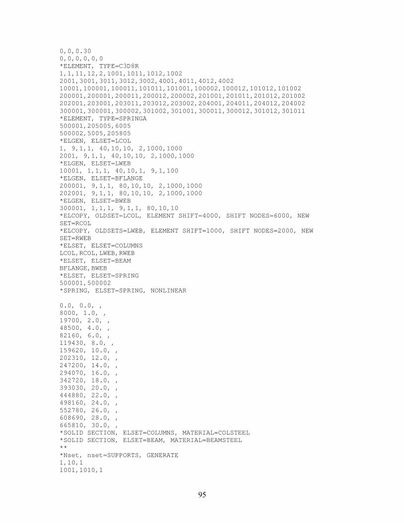
95
0,0,0.30 0,0,0,0,0,0 *ELEMENT, TYPE=C3D8R 1,1,11,12,2,1001,1011,1012,1002 2001,3001,3011,3012,3002,4001,4011,4012,4002 10001,100001,100011,101011,101001,100002,100012,101012,101002 200001,200001,200011,200012,200002,201001,201011,201012,201002 202001,203001,203011,203012,203002,204001,204011,204012,204002 300001,300001,300002,301002,301001,300011,300012,301012,301011 *ELEMENT, TYPE=SPRINGA 500001,205005,6005 500002,5005,205805 *ELGEN, ELSET=LCOL 1, 9,1,1, 40,10,10, 2,1000,1000 2001, 9,1,1, 40,10,10, 2,1000,1000 *ELGEN, ELSET=LWEB 10001, 1,1,1, 40,10,1, 9,1,100 *ELGEN, ELSET=BFLANGE 200001, 9,1,1, 80,10,10, 2,1000,1000 202001, 9,1,1, 80,10,10, 2,1000,1000 *ELGEN, ELSET=BWEB 300001, 1,1,1, 9,1,1, 80,10,10 *ELCOPY, OLDSET=LCOL, ELEMENT SHIFT=4000, SHIFT NODES=6000, NEW SET=RCOL *ELCOPY, OLDSETS=LWEB, ELEMENT SHIFT=1000, SHIFT NODES=2000, NEW SET=RWEB *ELSET, ELSET=COLUMNS LCOL,RCOL,LWEB,RWEB *ELSET, ELSET=BEAM BFLANGE,BWEB *ELSET, ELSET=SPRING 500001,500002 *SPRING, ELSET=SPRING, NONLINEAR 0.0, 0.0, , 8000, 1.0, , 19700, 2.0, , 48500, 4.0, , 82160, 6.0, , 119430, 8.0, , 159620, 10.0, , 202310, 12.0, , 247200, 14.0, , 294070, 16.0, , 342720, 18.0, , 393030, 20.0, , 444880, 22.0, , 498160, 24.0, , 552780, 26.0, , 608690, 28.0, , 665810, 30.0, , *SOLID SECTION, ELSET=COLUMNS, MATERIAL=COLSTEEL *SOLID SECTION, ELSET=BEAM, MATERIAL=BEAMSTEEL ** *Nset, nset=SUPPORTS, GENERATE 1,10,1 1001,1010,1

96
2001,2010,1 3001,3010,1 4001,4010,1 5001,5010,1 6001,6010,1 7001,7010,1 8001,8010,1 9001,9010,1 10001,10010,1 11001,11010,1 100002,100009,1 101002,101009,1 102002,102009,1 103002,103009,1 *Elset, elset=BLASTSIDE, GENERATE 1,9,1 11,19,1 21,29,1 31,39,1 41,49,1 51,59,1 61,69,1 71,79,1 81,89,1 91,99,1 101,109,1 111,119,1 121,129,1 131,139,1 141,149,1 151,159,1 161,169,1 171,179,1 181,189,1 191,199,1 201,209,1 211,219,1 221,229,1 231,239,1 241,249,1 251,259,1 261,269,1 271,279,1 281,289,1 291,299,1 301,309,1 311,319,1 321,329,1 331,339,1 341,349,1 351,359,1 361,369,1 371,379,1 381,389,1 391,399,1 *ELSET, ELSET=LCFO, GENERATE 1005,1395,10
97
*ELSET, ELSET=LCWL, GENERATE 10001,10040,1 *ELSET, ELSET=LCWR, GENERATE 10801,10840,1 *ELSET, ELSET=LCFI, GENERATE 2005,2395,10 *ELSET, ELSET=RCFI, GENERATE 5005,5395,10 *ELSET, ELSET=RCWL, GENERATE 11001,11040,1 *ELSET, ELSET=RCWR, GENERATE 11801,11840,1 *ELSET, ELSET=RCFO, GENERATE 6005,6395,10 *ELSET, ELSET=BTF, GENERATE 201005,201795,10 *ELSET, ELSET=BWT, GENERATE 300009,300799,10 *ELSET, ELSET=BWB, GENERATE 300001,300791,10 *ELSET, ELSET=BBF, GENERATE 202005,202795,10 *ELSET, ELSET=LCON, GENERATE 3355,3395,10 *ELSET, ELSET=LB, GENERATE 300002,300008,1 *ELSET, ELSET=RB, GENERATE 300792,300798,1 *ELSET, ELSET=RCON, GENERATE 4355,4395,10 *SURFACE, NAME=LCFO LCFO, S2 *SURFACE, NAME=LCWL LCWL, S1 *SURFACE, NAME=LCWR LCWR, S2 *SURFACE, NAME=LCFI LCFI, S1 *SURFACE, NAME=RCFI RCFI, S2 *SURFACE, NAME=RCWL RCWL, S1 *SURFACE, NAME=RCWR RCWR, S2 *SURFACE, NAME=RCFO RCFO, S1 *SURFACE, NAME=BTF BTF, S2 *SURFACE, NAME=BWT BWT, S4 *SURFACE, NAME=BWB BWB, S6 *SURFACE, NAME=BBF BBF, S1 *SURFACE, NAME=LCON LCON, S2 *SURFACE, NAME=LB
98
LB, S1 *SURFACE, NAME=RB RB, S2 *SURFACE, NAME=RCON RCON, S1 *TIE, NAME=BUILDSECTIONS LCWL,LCFO LCWR,LCFI RCWL,RCFI RCWR,RCFO BWT,BTF BWB,BBF *TIE, NAME=CONNECTIONS LB,LCON RB,RCON ** *AMPLITUDE, NAME=Blast, DEFINITION=TABULAR 0.0E-3, 0.0000, 1.0E-3, 1.0000, 2.0E-3, 0.7009, 3.0E-3, 0.4852 4.0E-3, 0.3307, 5.0E-3, 0.2207, 6.0E-3, 0.1433, 7.0E-3, 0.0893 8.0E-3, 0.0521, 9.0E-3, 0.0271, 10.0E-3, 0.0105, 11.0E-3, 0.0000 12.0E-3, -0.0064, 13.0E-3, -0.0100, 14.0E-3, -0.0116, 15.0E-3, -0.0121 16.0E-3, -0.0121, 17.0E-3, -0.0118, 18.0E-3, -0.0110, 19.0E-3, -0.0100 20.0E-3, -0.0089, 21.0E-3, -0.0078, 22.0E-3, -0.0067, 23.0E-3, -0.0058 24.0E-3, -0.0049, 25.0E-3, -0.0041, 26.0E-3, -0.0035, 27.0E-3, -0.0028 28.0E-3, -0.0021, 29.0E-3, -0.0014, 30.0E-3, -0.0007, 31.0E-3, -0.0000 ** ** MATERIALS ** *Material, name=COLSTEEL *Density 0.0007379 *Elastic 29000000, 0.3 *Plastic 50000, 0.0000 *RATE DEPENDENT,TYPE=YIELD RATIO 1.000,0.000000 1.046,0.001 1.074,0.002 1.092,0.003 1.116,0.005 1.153,0.01 1.192,0.02 1.216,0.03 1.247,0.05 1.291,0.10 1.337,0.20 1.364,0.30 1.399,0.50 1.447,1 1.495,2 1.523,3 1.558,5 1.605,10 1.655, 20 1.683, 30 1.718, 50

99
1.767, 100 1.815, 200 1.843, 300 ** *Material, name=BEAMSTEEL *Density 0.0007334 *Elastic 29000000, 0.3 *Plastic 50000, 0.0000 *RATE DEPENDENT,TYPE=YIELD RATIO 1.000,0.000000 1.046,0.001 1.074,0.002 1.092,0.003 1.116,0.005 1.153,0.01 1.192,0.02 1.216,0.03 1.247,0.05 1.291,0.10 1.337,0.20 1.364,0.30 1.399,0.50 1.447,1 1.495,2 1.523,3 1.558,5 1.605,10 1.655, 20 1.683, 30 1.718, 50 1.767, 100 1.815, 200 1.843, 300 ** ** STEP: Blast ** BOUNDARY CONDITIONS ** ** Name: Fixed Support ** *STEP, NLGEOM=YES Blast Load *DYNAMIC, EXPLICIT , 0.25, , 0.001 *Boundary SUPPORTS, ENCASTRE *DLOAD, AMPLITUDE=Blast BLASTSIDE, BX, 4000 ** ** OUTPUT REQUESTS ** *OUTPUT, FIELD, VARIABLE=PRESELECT, NUMBER INTERVAL=50 *OUTPUT, HISTORY, VARIABLE=PRESELECT *END STEP

100
Appendix C
Comparison of Time Histories of the Bilinear and Nonlinear Spring
Forces Resulting from a 4,000 psi Blast

101
C.1 Comparison of Time Histories of Bilinear and Nonlinear Spring Forces
0
10
20
30
40
50
60
0 0.03 0.06 0.09 0.12 0.15
Time, sec
Spri
ng F
orce
, kip
2 kip/in. 1̂.3 spring 5 kip/in. spring 2.5 kip/in.^1.3 spring Fig. C.1. Comparison of time histories of 5 kip/in. bilinear and corresponding nonlinear
spring forces for frame subjected to a 4,000 psi blast
0
30
60
90
120
150
0 0.03 0.06 0.09 0.12 0.15
Time, sec
Sprin
g Fo
rce,
kip
8 kip/in. 1̂.3 nonlinear spring 20 kip/in. spring 10 kip/in. 1̂.3 nonlinear spring Fig. C.2. Comparison of time histories of 20 kip/in. bilinear and corresponding nonlinear
spring forces for frame subjected to a 4,000 psi blast

102
Vita
Michael Rembert Motley was born in Charleston, South Carolina on April 20, 1982,
where he lived for the duration of his youth, graduating from St. Andrew’s Parish High
School in June 1999. He attended The Citadel in Charleston from 1999 to 2003 where he
received his Bachelor of Science Degree in Civil and Environmental Engineering. He
moved on to Virginia Polytechnic Institute and State University as a Via Fellow in the
summer of 2003 where he continued his studies in pursuit of a Master of Science Degree
in Structural Engineering in the Via Department of Civil and Environmental Engineering.
He completed his Master’s Degree program in December of 2004.
______________________
Michael R. Motley