finite element analysis of braided corrugated hoses with

1

WHITE PAPER

/ IntroductionWhile explicit solvers have been used to analyze corrugated braided hoses with only a single layer of braid wires, the Ansys implicit solver can perform finite element analysis of braided corrugated hoses with multiple layers of braid wires. An implicit solver can perform both static and transient analyses. In general, implicit solvers provide more accurate solutions and solve static or quasi-static analyses more efficiently than explicit solvers. Read this white paper to learn the detailed physics of braided corrugated hoses, as well as the challenges that engineers face in designing them for specific applications.

/ Current State of the Art Regarding Finite Element Analysis of Metallic Braided Corrugated Hoses

Until recently, stress analysis of braided corrugated hoses has been performed primarily using hand calculations, experimental test data and computer programming. Some flexible hose analysts follow the design guidelines presented in the EJMA Standard, published by the Expansion Joint Manufacturers Association, Inc. EJMA is an association of manufacturers of metal bellows type expansion joints. Their website http://www.ejma.org/ states that they “carry out extensive technical research and testing on many important aspects of expansion joint design and manufacturing.”

Over the years, a number of papers and theses concerning analysis of expansion joints have been published. Many of those papers were published before finite element analysis software became widely available. Some of the earlier papers concentrated on analyzing one portion of a system instead of analyzing an entire assembly of components. Analysis of U-Shaped Expansion Joints(1) which was published during 1962 describes “An elastic analysis of U-shaped expansion joints under axial loads and internal or external pressure is presented. The general solution permits the investigation of any U-shaped expansion joint falling in the range of thin shells, for any arbitrary combination of axial forces and pressure loading.”

Finite Element Analysis of Braided Corrugated Hoses with Multiple Layers of Individual Braid Wires Using an Ansys Implicit Solver //

This white paper demonstrates the Ansys implicit software package is robust for performing finite element analysis of multi-layered braided corrugated hoses. This paper outlines the methodology for creating and analyzing three-dimensional finite element hose models consisting of an inner metallic corrugated tube or flexible bellows which is surrounded by either a single braid layer or multiple braid layers of helically wound, circular, individual metallic wires.

Finite Element Analysis of Braided Corrugated Hoses with Multiple Layers of Individual Braid Wires Using an Ansys Implicit Solver

Figure 1. Two mesh elements through the corrugated tube wall thickness.

2Finite Element Analysis of Braided Corrugated Hoses with Multiple Layers of Individual Braid Wires Using an Ansys Implicit Solver //

Furthermore, the paper states, “The method presented here lends itself readily to programming on an electronic computer.”

This paper is useful for performing an analysis of U-shaped expansion joints, which is basically what a corrugated tube is. Unfortunately, the methods discussed do not extend to analysis of braided corrugated hoses with single or multiple layers of braid wires. Unless the wall thickness of a corrugated tube is sufficiently thick, at some point the bellows will excessively stretch, deform and squirm. Adding multiple layers of braid wires to a corrugated tube or bellow extends the range of axial loads and pressure which can be sustained before bellows failure occurs. The analysis methods presented in Analysis of U-Shaped Expansion Joints are limited to analyzing a U-shaped expansion joint at a relatively low pressure and corresponding axial hose pressure force. Those methods are also restricted to geometrical shell thickness limits.

Even within the past several years, instead of analyzing flexible corrugated hoses with multiple layers of braid wires and treating each braid wire as an individual component, some analysts (2) modeled picks of parallel braid wires as “ribbons” of wires with composite material properties.

By modeling a grouping of wires as a ribbon, each wire within a ribbon is essentially bonded or welded to its neighbor. In the real world, individual braid wires slide and flex freely relative to each other. That’s why it’s important to be able to perform finite element analysis of braided corrugated hoses where each braid wire is modeled as an individual three-dimensional component which can move independently.

During 2015, Djihad Rial, Amine Tiar, Kebir Hocine, Jean-Marc Roelandt and Eric Wintrebert authored Metallic Braided Structures: The Mechanical Modeling(3) documenting their finite element analysis results of “a micro-scale model where each metallic wire is considered an independent three-dimensional structure.”

Rial et al, used an explicit type finite element analysis solver. Explicit solvers utilize a “dynamic” or time-domain type of solver. They evaluated several different braided corrugated hose modeling techniques and compared their finite element analysis results with experimental test data from elongation and pressurized hose tests.

The following quotation is from Metallic Braided Structures:

“… several finite element approaches were developed and compared with the experiment, which are: a micro-scale model where each metallic wire is considered as an independent three-dimensional structure, a meso-scale model where each group of wires was modeled as a continuum material with equivalent mechanical behavior, and a macro-scale model where the whole structure is considered as a fully homogeneous material. And it is shown that the homogenization is more suitable for small displacements but for complex behavior the meso- and the micro-scale models are more reliable.”

A continuum model is basically a “composite” model, whereby composite material properties are assigned to a collection of components, typically to simplify finite element model creation and analysis. The resulting stress, strain, force and moments from a continuum hose model are less accurate than those obtained from a three-dimensional micro-scale model of a braided corrugated hose with individual braid wires.

Figure 2. Beam mesh elements – Each circular beam segment contains 16 mesh elements.

Figure 3. Circular beam and mesh elements are graphically displayed by Ansys using an octagonal outline.


/ Flexible Braided Corrugated Hose Design Braided corrugated hoses are used in many applications, including plumbing, industrial, automotive and aerospace/rocket applications. Braided corrugated hoses have an internal, semi-flexible, metallic corrugated tube or bellows, which is surrounded by either a single layer or multiple layers of metallic, individual braid wires. The braid wires are grouped into picks, which are bundles of parallel wires which follow alternating helical, CW and CCW paths. The metallic corrugated tube provides flexibility, allowing the braided hose assembly to compress, elongate, bend and flex.

Hose connection fittings which are often threaded, are welded to both ends of a typical hose assembly. Hollow, concentric sleeves, which are overlapping collars, surround the ends of the braid wire tips. The ends of the braid wires are welded to the ends of the corrugated tube and to the weld collars. Then the hose connection fittings are welded to the weld collars. The ends of a hose assembly are extremely stiff compared to the rest of the more flexible, braided corrugated section.

Braid wires protect the flexible corrugated tube from external scuffing and abrasion. Additionally, the braid wires are intended to prevent a pressurized hose failure mode which is called “squirm.” Whenever a braided hose is over-pressurized, the corrugated tube bellows can elongate and a portion of the bellows can squirm, bulging and pushing aside the braid wires. When squirm occurs, the bulging portion of a bellows can burst. Hose manufacturers specify safe operating pressure limits so that squirm does not occur within normal operating pressure limits. A manufacturer’s hose operating pressure rating is typically established by pressurizing a hose until it bursts and then dividing the burst pressure by four.

/ Finite Element Analysis Modeling Considerations

Modeling and “contact” finite element analysis of braided corrugated hoses is extremely complicated. Wires within a pick contact adjacent wires. Wires within a braid layer contact wires in adjacent braid layers. Wires within the innermost braid layer contact the curved crest surfaces on the outside of the corrugated tube. Wire-to-wire sliding between picks and wire-to-tube sliding involves friction. Friction and contact are both non-linear, finite element analysis modeling phenomena. As the braid wires stretch and elongate, their material properties can also behave nonlinearly, becoming more elastic or possibly even elastic-plastic. Braided hose contact finite element analysis is extremely nonlinear and difficult to model. It’s also computationally expensive.

The diameters of the braid wires and the wall thickness of the corrugated tube are very small in comparison to the axial hose length. For performing contact finite element analysis, it’s best to incorporate at least two mesh elements “through” the thickness of the corrugated tube wall. Multiple mesh elements are also required across the diameter of each braid wire. The meshes for the corrugated tube and the braid wires require a very large number of nodes and elements.

Large finite element models with lots of nodes and elements take a long time to solve.

Although the braid wire beam elements have a circular cross-section, Ansys displays these circular beam elements with an octagonal outline.

Using the “esurf” command, Ansys inserts a layer of contact surface elements between contacting beams and between beams and contact surfaces. These specialized contact surface elements perform a number of functions. One of their main functions is to keep track of the distance between nearby element surfaces, as they approach, come into contact and

Figure 4. Wire “pass-through.”

Figure 5. Single braid layer with 2-over and 2-under braid weave pattern.

Figure 6. Smooth and kinked braid weaves with 2 wires-per-pick.


separate from each other. Whenever the contact status changes, additional load step iterations are required before the step converges satisfactorily. These additional “contact status change” iterations significantly increase the computational time required for analysis.

During a FEM load iteration step, whenever two objects or surfaces contact each other, they could potentially “pass-through” or “tunnel-through” each other. Physically, wires can’t pass through other wires, nor can metallic wires pass through a metallic corrugated tube, but this phenomenon could occur during a finite element (mathematical) model simulation. To prevent pass-through or tunneling, penalty-based contact elements (acting as springs) are employed to inhibit excessive contact penetration. These contact elements only exist mathematically. They do not have any mass or weight. It’s important to be aware that the esurf surface mesh layer cannot be displayed graphically by the Ansys GUI.

A slight amount of contact interference or penetration is required for the penalty method to function. Good finite element analysis modeling techniques result in a minimal amount of surface-to-surface penetration under load. If the load step is large enough, or if the load step is applied too quickly, then individual beam elements could: pass-through other beams, pass-through the corrugated tube or severely distort the corrugated tube mesh, crushing and collapsing it.

/ Braid Diameter O.D. Modeling ConsiderationsWhen the innermost layer of braid wires maintains line-to-line contact with the outside diameter of the corrugated tube crests, the theoretical minimum outside diameter (TMOD) of a single braid layer is equal to the corrugated tube outside diameter plus four times the nominal braid wire diameter. Due to manufacturing tolerances and variances in braid wire carrier tensioning, the actual braid outside diameter (ABOD) will likely be larger than this theoretical minimum value. ABOD is a critical geometrical braid weave modeling dimension or parameter, affecting the steepness/smoothness of the undulating braid profile.

/ Helical Braid Generator Software PackagesThere are several commercially available helical braid generator software packages.

/ TexMind SoftwareAccording to the TexMind website, http://texmind.com/wp/, “TexMind BraiderTM is an intuitive CAD-Software for colour and structural design of standard tubular and flat braids.” Although the TexMind website advertises “Software and Consulting for Textiles,” the TexMind Braider software package can also generate small diameter, metallic braid weave wire geometry. The TexMind software exports braid geometry into several finite element analysis software packages.

/ GiD Software“https://www.gidhome.com/ is a universal, adaptive and user-friendly pre and postprocessor for numerical simulations in science and engineering.”

According to A CAD Tool for Electromagnetic Modeling of Braided Wire Shields(4) GiD has a module with a graphical user interface for creating “braided wire CAD geometry.”

One of the input variables within the GiD graphical user interface (GUI) λmedium, specifies the “distance between carriers.” This is equivalent to specifying the distance between “crossing” braid wires. So, while using the GiD graphical user interface, an analyst could theoretically specify line-to-line contact between braid wires or a specific amount of clearance between picks of crossing wires.

From the web-based document, A Finite Element Tool for the Electromagnetic Analysis of Braided Corrugated Shields(5) “input values for specifying a smoother or steeper ascent/descent of the wires” can be specified from the GiD user interface.

According to A Finite Element Tool: “A previous step before starting with the numerical analysis is to generate a CAD geometry representing the braided wire shield. In our case, this task is performed with a Tcl/TK plug-in integrated in the pre-processor software GiD.”

This plug-in module essentially creates a small portion of the geometry for two picks of crossing braid wire sets which is referred to as a “unit cell.” From A Finite Element Tool “the full braided geometry is generated after rotating the unit cells in the transversal planes and translating them along the longitudinal axes.”

The unit cell contains a small snippet of braid wire geometry. This repeatable snippet of geometry is copied and rotated around the longitudinal axis, and then shifted axially, as many times as required in order to create a full complement of braid wires.

A Finite Element Tool states “The parameter λC determines the maximum vertical (transversal) distance between carriers… an estimation of this parameter has to be made based on the other braid parameters such as weave angle, strand diameter and braid diameter.”

https://www.gidhome.com/


It appears that while using the GiD plug-in, an analyst would specify a desired value for λC. Then it appears to be necessary to visually inspect the resulting three-dimensional CAD geometry to make sure that none of the braid wires have interpenetrated each other. If the resulting three-dimensional CAD representation indicates wire-to-wire interpenetration, the analyst would need to enter another value for λC and repeat this process as many times as required until satisfied with the resulting CAD geometry.

Regarding the two web-based documents which were just mentioned, the expression λC is equivalent to λmedium which is the distance between (braid wire) carriers. It’s important to understand that when an analyst uses the GiD graphical interface and enters a specific value for λmedium that it may not be possible for the software to create a unit cell using that specific value because the value for λmedium is dependent on other input parameter values. The significance of λmedium which is the distance between carriers or the distance between crossing wires will become clearer after reading the next section.

/ Universal Helical Braid Wire Generator Software

The author of this white paper created a “universal” helical braid wire generator software package for creating alternating helical braid wire profiles. The generator creates continuous smooth braid profile wire paths as well as steeper, linear or “kinked” wire profiles.

The braid generator software outputs a series of consecutive X, Y, and Z data points in 3D space, tracing the helical paths for the centerlines of individual braid wires. Then, a circular cross-section is extruded along the entire length of each braid wire path or profile, creating a quasi-smooth braid weave solid model. The braid generator software acts like a pre-processer for a CAD modeler. Alternatively, the generated data points can be imported directly into a finite element analysis modeler, which would then be used to create the individual braid wire extrusions.

For finite element modeling purposes, a smooth, continuous, braid weave profile is preferred over a linear/kinked wire path. If the braid weave wire profile is too steep or linear, then the FEA wire mesh elements may contain sharp facets or discontinuities. Sharp mesh facets can result in troublesome residual force hotspots during finite element analyses, causing simulations to terminate prematurely.

The author’s braid generator software creates helical braid wire paths. This software allows an analyst to specify a minimum distance between crossing wires. Line-to-line contact between crossing wires can also be specified. When line-to-line contact is specified, none of the crossing wires will penetrate each other. Some of the crossing wires will result in line-to-line contact while other nearby crossing wires will have a very slight amount of clearance between them. It’s not possible for all of the crossing wires to be line-to-line.

Figure 7 shows line-to-line contact with five decimal places accuracy between “Pick No. 2 – wire L2 and Pick No. 1 – wire L2” and also between “Pick No. 4 – wire R2 and Pick No. 1 – wire R2.” The maximum clearance between crossing wires = 0.00173”. The average clearance between all crossing wires is approximately 0.001”.

Figure 8 shows two crossing wires with line-to-line contact while nearby crossing wires have a minimal amount of clearance.

Figure 9 illustrates line-to-line contact for crossing wires and line-to-line contact for parallel wires within a pick of braid wires. Notice that each wire end within a pick is intentionally staggered axially.

Figure 7. Distances between crossing braid-wire centerline.

Figure 8. Line-to-line contact and slight clearance between nearby crossing wires.

Figure 9. Line-to-line contact between crossing wires and parallel wires.


Mathematically, if any of the braid wire geometries initially penetrate each other, which could possibly occur from a model which was incorrectly generated, either by mathematical modeling or from 3D CAD, then the FEA contact model would not be able to initialize properly. For contact finite element analysis, it’s extremely important that the helical braid wire generator software ensures line-to-line contact between parallel and crossing braid wires or some amount of clearance between them.

The author’s braid generator software employs “skew line” mathematical calculations between the centerlines of crossing wires. Using an iterative, bi-section modeling technique, the braid weave profile paths are automatically adjusted to obtain line-to-line contact or to provide a specific minimum amount of clearance between crossing wires.

As mentioned earlier, the universal braid generator outputs a series of consecutive X, Y, and Z data points in three-dimensional space. Ansys WorkbenchTM imports these data points and creates curves connecting the data points. A circular profile is then extruded along the curve centerlines, creating a quasi-smooth, braid weave solid model. Since the underlying helical wire curves are composed of discrete points, each section of braid wire geometry between any two data points is essentially a line segment.

“Two non coplanar lines are called skew lines if they are neither parallel nor intersecting. For skew lines, the direction of shortest distance is perpendicular to both the lines.”[6]

The shortest distance between any two skew lines can be determined mathematically by solving vector equations. The author’s helical braid generator software calculates the shortest distance between all of the crossing braid wire line segments. By subtracting the braid wire diameter from the skew line distances, the braid generator software automatically determines the amount of clearance or interference between crossing wire line segments.

A Visual Basic macro within the braid generator software can automatically adjust the value of the exponent b in the following formula y = a * √(xb) + radlowest

Where:

y = radial distance from the hose axial centerline

x = axial distance from the start of the braid weave cycle

a = radial “height” scaling factor for one-quarter cycle,

a = (radmiddle - radlowest)/ √[(xpointNo8)b]

radlowest = corrugated tube outside radius + braid wire radius

radmiddle = radius at mid-point of total radial rise

xpointNo8 = axial distance for braid Point No. 8 from the start of the braid weave cycle

x0 is the first x value

Note: when x = xpointNo8, y = radmiddle

By design, some of the crossing wires between braid wire picks will be line-to-line while nearby crossing wires will have some minimal amount of clearance between them. This guarantees that none of the braid wires will initially interpenetrate each other geometrically when the finite element analysis begins. An additional benefit of a tight braid weave is that it reduces chatter which can occur whenever the “contact element status changes” during finite element analysis.

The formula y = a * √(xb) + radlowest is used only for the first quarter of a 360° helical cycle. For the next quarter cycle, the values for the y increment are mirrored about the midpoint of the total radial rise. This process is repeated for the third and fourth quarter cycles, creating a smooth, continuous braid weave profile.

Figure 10. 360° braid weave profile – for 1st quarter cycle where y = a * √(x9) .


By changing the value for parameter b in the formula y = a * √(xb) the “linear ascent/descent” or steepness of the braid weave profile can be adjusted to mimic the range of profiles shown in the following figure. When b ~ 1.875, the braid weave profile is similar to a saw-tooth profile. The steepest braid weave profile occurs when b ~ 40. Smooth profiles occur when b is between 2 and 14. As the parameter b increases, the curve profile becomes steeper. Steeper braid profiles allow more wires to be packed into a braid layer.

A schematic of the author’s helical braid wire generator algorithm is shown in Figure 12. After entering the input parameters, the analyst manually selects and adjusts the value for the parameter b until visually satisfied with the steepness or smoothness of the radii curve profile.

If line-to-line contact or satisfactory clearance results, a macro can automatically output the X, Y and Z data point files.

If line-to-line contact does not occur or if the clearance between crossing wires is not satisfactory, there are two options:

1. Increase the value of the actual braid outside diameter, ABOD, which was discussed previously. Either the analyst can manually input a new value for ABOD or a macro can be used to automatically determine the optimum value so that line-to-line contact occurs between crossing wires.

2. Either manually input a new value for b or use a macro to automatically determine the parameter b which results in line-to-line contact between crossing wires or a minimum amount of clearance specified by the analyst.

Figure 11. 360° helical braid weave profiles.

Figure 12. Universal helical braid wire generator software algorithm schematic.


The author’s helical braid generator uses symmetry concepts which are similar to the unit cell method discussed in A CAD Tool for Electromagnetic Modeling of Braided Wire Shields(4) and A Finite Element Tool for the Electromagnetic Analysis of Braided Corrugated Shields.(5) Instead of using the unit cell method, the author’s braid generator rotates each braid wire within a pick around the hose axis and shifts each wire axially relative to its adjacent neighbor. The universal braid generator software uses helical angular rotation about the hose axis as the main driving mathematical formula. Although this is slightly more complicated than a unit cell method, the main benefit is that skew line mathematical calculations can be implemented by the braid generator software to enforce line-to-line contact of crossing wires, preventing geometrical wire-to-wire penetration.

/ Ansys SoftwareFor the forced deflection elongation models and the pressurized hose finite element models documented within this paper, the author utilized Ansys Academic software. The maximum number of components which can be created using an Ansys Academic license is limited to 50 components. The corrugated tube geometry is split into two components along the hose longitudinal axis. All the models created using the Ansys Academic software are limited to a maximum of 48 individual braid wire components.

As an “Ansys Associate,” the author previously had temporary access to Ansys Professional software and one HPC pack. Ansys Professional was used to create longer hose models with more wires per braid layer than those which are documented within this white paper. During that time frame, larger finite element models with more wires did not converge satisfactorily due to residual force tolerance issues. Those residual force tolerance issues have been overcome and the modeling techniques which were used to overcome them will be discussed later in this paper.

/ Nomenclature: Parallel and Crossing BeamsParallel wires within a pick of braid wires are bundled parallel to each other. Crossing picks of braid wires cross each other at an angle

KEYOPTS (for 3D line contact element CONTA177)

KEYOPT commands allow an analyst to specify contact options which may or may not be available directly through the Ansys GUI.

KEYOPT(3) specifies the type of traction based model to be implemented by Ansys for contact.

KEYOPT(3)=2 Parallel and crossing beams contact traction-based model KEYOPT(3)=3 Crossing beams contact traction-based model

In order to prevent beam-to-beam penetration for both “parallel and crossing beams” Ansys created KEYOPT(14)=1 and KEYOPT(14)=2.

KEYOPT(14)=1, Parallel or crossing beams

Option 1 keeps track of up to 4 (parallel or crossing) beam contacts KEYOPT(14)=2, Parallel or crossing beams

Option 2 keeps track of up to 8 (parallel or crossing) beam contacts

Figure 14 shows beam elements which are simultaneously “parallel and crossing.” Four of the beam elements are parallel to each other and one beam element crosses the other four.

KEYOPT(3)=2 Parallel and crossing beams contact traction based model should also be used whenever KEYOPT(14) is specified.

Figure 13. Illustration of two picks of crossing wires containing five parallel wires-per-pick.

Figure 14. Illustration of KEYOPT(14).

Figure 15. Named selection End_Z_1pt2_inner_braid.


For single, dual and triple braid layer models analyzed using Ansys Academic, all the models contain 48 braid wires with as many as 4 wires-per-pick. KEYOPT(14)=1 was sufficient to prevent excessive beam-to-beam penetration for models with 4 wires-per-pick. Using KEYOPT(14)=2 doubled the time for solving the models without offering any noticeable benefit. KEYOPT(14)=2 might be useful for analyzing braided corrugated hose models containing more than 4 wires-per-pick.

/ Method for Creating Braided Corrugated Hose Models The corrugated profile for one-half of the tube is created using Ansys WorkbenchTM. The U-shaped corrugation profile is revolved 180° around the hose axis centerline. Then a mirror copy of the half-tube is created.

Picks of braid wire X, Y, and Z data point curves are imported into Ansys WorkbenchTM. The ends of the braid wires are shifted axially to align with the ends of the corrugated tube. A circular profile is extruded along each braid wire curve. Additional picks of extruded braid wires are then copied and rotated as required. This method of “copying and rotating” picks of wires is similar to the unit cell approach employed by the GiD software.

/ Corrugated Tube and Braid Wire Dimensions and MaterialsThe materials and dimensions for the corrugated tube and the braid wires are shown below.

The Ansys default stainless steel material properties (30,458 psi yield stress) were used for axial hose elongation, tip deflection and tri-axial deflection models. For the pressurized hose models, 316 stainless steel material properties (42,100 psi yield stress) were used.

/ Mesh GenerationFor the corrugated tube, a sweep method was used to create a linear quad solid element mesh. Two mesh elements were specified through the wall thickness of the corrugated tube. Mid-side nodes were not activated. The mesh length was specified for the braid wires.

/ Named SelectionsNamed selections are created using the Ansys WorkbenchTM GUI so that bodies, faces and node sets can be specified later. The named selections are subsequently used to specify contact element pairs within Ansys command scripts.

An example of a named selection is shown in Figure 15. The named selection “End_Z_1pt2_ inner_braid” is a set of braid wire nodes. This node set is used to bond the ends of the inner braid wires to the end of the corrugated tube, simulating a welded connection.

/ Ansys Command ScriptsAnsys command scripts are created for specifying

1. Attachment/bonding of the braid wire ends to the ends of the corrugated tube.

2. Beam-to-beam contact within braid layers.

3. Beam-to-beam contact between adjacent braid layers.

4. Beam-to-surface contact between the innermost braid layer and the corrugated tube crest surfaces.

Material Wall Thickness or Diameter (in)

Axial Length (in) Inside/Outside Diameter (in)

Corrugated Tube Stainless Steel 0.012 1.20 0.375/0.590

Braid Wires Stainless Steel 0.016 1.20 N/A

Table 1. Corrugated Tube and Braid Wire Dimensions and Materials.


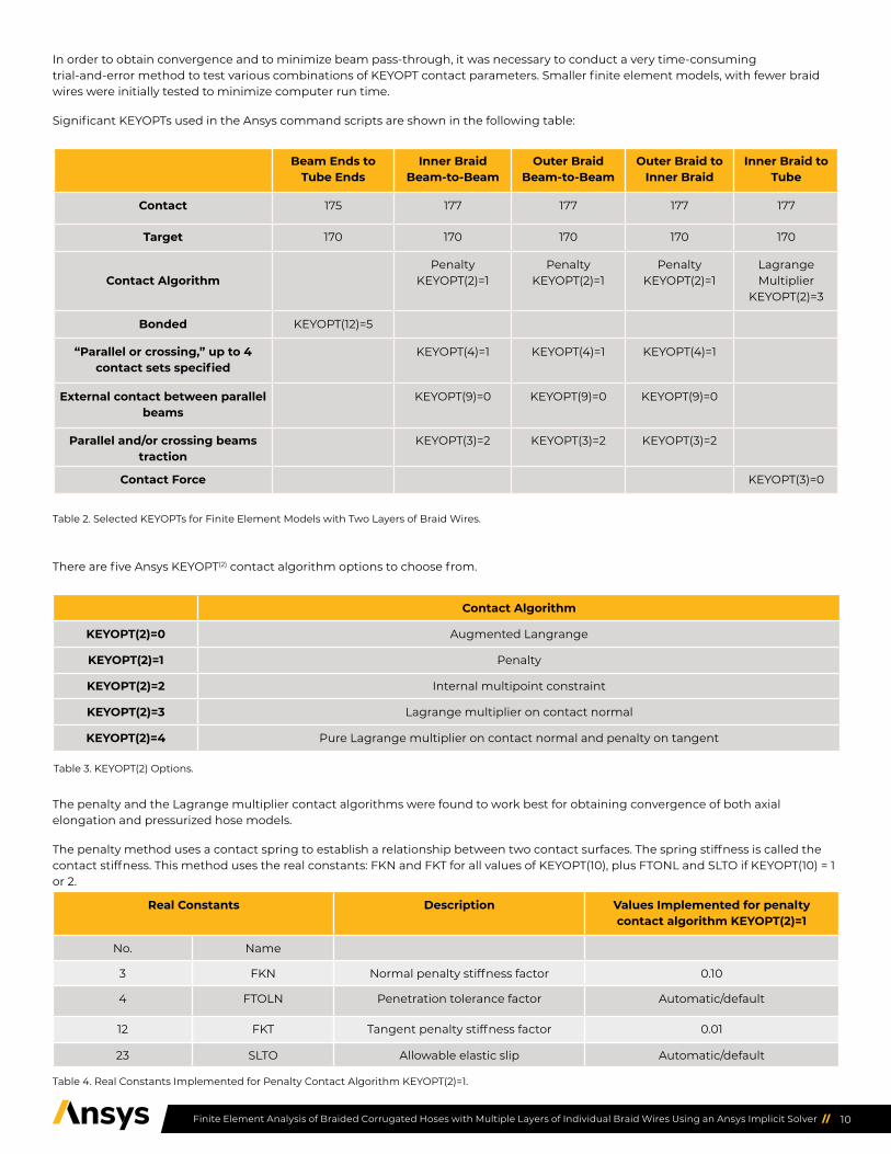
In order to obtain convergence and to minimize beam pass-through, it was necessary to conduct a very time-consuming trial-and-error method to test various combinations of KEYOPT contact parameters. Smaller finite element models, with fewer braid wires were initially tested to minimize computer run time.

Significant KEYOPTs used in the Ansys command scripts are shown in the following table:

There are five Ansys KEYOPT(2) contact algorithm options to choose from.

The penalty and the Lagrange multiplier contact algorithms were found to work best for obtaining convergence of both axial elongation and pressurized hose models.

The penalty method uses a contact spring to establish a relationship between two contact surfaces. The spring stiffness is called the contact stiffness. This method uses the real constants: FKN and FKT for all values of KEYOPT(10), plus FTONL and SLTO if KEYOPT(10) = 1 or 2.

Beam Ends to Tube Ends

Inner Braid Beam-to-Beam

Outer Braid Beam-to-Beam

Outer Braid to Inner Braid

Inner Braid to Tube

Contact 175 177 177 177 177

Target 170 170 170 170 170

Contact AlgorithmPenalty

KEYOPT(2)=1Penalty

KEYOPT(2)=1Penalty

KEYOPT(2)=1Lagrange Multiplier

KEYOPT(2)=3

Bonded KEYOPT(12)=5

“Parallel or crossing,” up to 4 contact sets specified

KEYOPT(4)=1 KEYOPT(4)=1 KEYOPT(4)=1

External contact between parallel beams


Parallel and/or crossing beams traction


Contact Force KEYOPT(3)=0

Table 2. Selected KEYOPTs for Finite Element Models with Two Layers of Braid Wires.

Contact Algorithm

KEYOPT(2)=0 Augmented Langrange

KEYOPT(2)=1 Penalty

KEYOPT(2)=2 Internal multipoint constraint

KEYOPT(2)=3 Lagrange multiplier on contact normal

KEYOPT(2)=4 Pure Lagrange multiplier on contact normal and penalty on tangent

Table 3. KEYOPT(2) Options.

Real Constants Description Values Implemented for penalty contact algorithm KEYOPT(2)=1

No. Name

3 FKN Normal penalty stiffness factor 0.10

4 FTOLN Penetration tolerance factor Automatic/default

12 FKT Tangent penalty stiffness factor 0.01

23 SLTO Allowable elastic slip Automatic/default

Table 4. Real Constants Implemented for Penalty Contact Algorithm KEYOPT(2)=1.


The Lagrange multiplier method is applied on the contact normal and the penalty method (tangential contact stiffness) is applied on the frictional plane. This method enforces zero penetration and allows a small amount of slip for the sticking contact condition. It requires chattering control parameters, FTONL and TNOP, as well as the maximum allowable elastic slip parameter SLTO.

Note: TNOP defaults to the force convergence tolerance divided by contact area at contact nodes. Additional KEYOPT settings are shown in Table 6.

The “sweet spot” for contact friction values was determined by trial-and-error to between 0.10 and 0.25. Friction values beyond this range sometimes caused convergence problems such as contact “chattering” or longer computer run time. A friction value of 0.25 was utilized for all finite element models documented in this paper.

The following table shows Ansys analysis setting options implemented so that models converge satisfactorily.

Real Constants Description Values Implemented for penalty contact algorithm KEYOPT(2)=1

No. Name

3 FKN Normal penalty stiffness factor 0.70

4 FTOLN Penetration tolerance factor -0.001

12 FKT Tangent penalty stiffness factor 0.01

23 SLTO Allowable elastic slip Automatic/default

24 TNOP Maximum allowable tensile contact pressure

Automatic/default

Table 5. Real Constants Implemented for Penalty Contact Algorithm KEYOPT(2)=3.

KeyOPT No. Description

KEYOPT(6)=2 Contact stiffness variation - aggressive

KEYOPT(10)=2 Normal contact stiffness - updated at each iteration

KEYOPT(15)=2 Contact stabilization damping - activated for all load steps

Table 6. KEYOPTS Implemented within Many of the Ansys Command Scripts.

Material Property Description Values Implemented

Mp, mu, mt 0.25 Coefficient of friction 0.25

Table 7. Material Property Value Utilized for Coefficient of Friction.

Description Option selected

Analysis type Static

Non-linear geometric effects On

Equation solver option Sparse

Elastic material properties included Yes

Newton-Raphson option Program chosen

Globally assembled metrix Symmetric

Nonlinear stabilization On (constant)

Stress-stiffening On

Weak springs On

Table 8. Ansys Analysis Settings.


/ Deflection (Axial Tension) Finite Element ModelsDeflection finite element models with single, dual and triple layers of braid wires (containing a total of 48 wires per model) were analyzed. For the dual and triple layer FEMs, the forced deflection magnitude was increased until either:

1. Braid wires passed-through the corrugated tube.

2. Braid wire mesh and/or the corrugated tube mesh collapsed or imploded.

For the single braid layer finite element model, when a forced deflection of 0.5 inch was applied, the braid wires still did not pass through the corrugated tube. Since the original hose length was 1.2 inches long, 0.5” deflection corresponds with a strain rate of approximately 42%. For stretching of this magnitude the braid wire material properties moved into the elastic-plastic range.

The single braid layer finite element model can stretch beyond 0.500”. The dual braid layer finite element model can stretch up to 0.156” before the innermost braid wires pass through the corrugated tube bellows. The triple braid layer model stretches 0.125” before excessive wire-to-tube penetration occurs.

Examination of the axial forces from the models containing multiple braid layers shows the innermost braid layer carries a substantially larger axial force per wire than subsequent braid layers. The resulting axial forces in the innermost braid layer wires are the highest, followed by those in the second and third braid layers.

Ansys deflection videos show that when hose axial tension deflection first begins, the innermost braid layer quickly compresses against the corrugated tube crests. As additional axial hose elongation occurs, the second layer of braid wires compress against the innermost layer of braid wires. As further axial hose deflection takes place, the third braid layer wires compress against the second layer of braid wires.

Although it may seem intuitive, the braid-wire-to-tube-crest radial compression is initially the severest at the midpoint of the hose. As hose elongation increases, the radial compression zone expands axially.

The wires within the innermost braid layer carry the largest axial forces compared to the other layers. At extreme hose pressure limits, the innermost braid layer wires carry a significantly larger percentage of the total axial wire forces.

It is interesting that the hose axial stiffness for the single, dual and triple layer FEMs are nearly identical at their maximum axial deflection limits.

Figure 16 shows a 1.2-inch-long single braid layer corrugated hose FEM before and after being stretched 0.5 inch. The sectioned views show the braid wires contacting and squeezing against the corrugated tube crests.

FEM Description Single Layer Two Layers Three Layers

Total No. of braid wires 48 48 48

No. of picks per braid layer 12 12 16

No. of wire-per-pick 4 2 1

No. of braid layers 1 2 3

Input (1) Hose axial deflection (limit) 0.500” 0.156” 0.125”

Output Reaction force 611 lbf 214 lbf 154 lbf

Hose axial stiffness 1,222 lbf/inch 1,371 lbf/inch 1,232 lbf/inch

Table 9. Forced Deflection (Tension) Reaction Forces for Models with 48 Braid Wires.(1)(1) 316 stainless steel (30,458 psi yield stress)


/ Pressurized Hose ModelsWhen a braided corrugated hose is internally pressurized, hose pressure forces are exerted in both the radial and axial directions. The axial hose pressure force is equal to the internal hose pressure multiplied by the hose flow area. Some analysts refer to the axial hose pressure force as the “plug” force.

As hose pressure increases, the axial hose force increases nonlinearly according to the formula:

f=p * π r2

Where:

f = axial hose pressure force (lbf) p = internal hose pressure (psi)

r = corrugated tube inner radius (in)

The axial hose pressure force stretches the bellows corrugations and the braid wires, causing wires to squeeze or compress against the corrugated tube bellows crest surfaces.

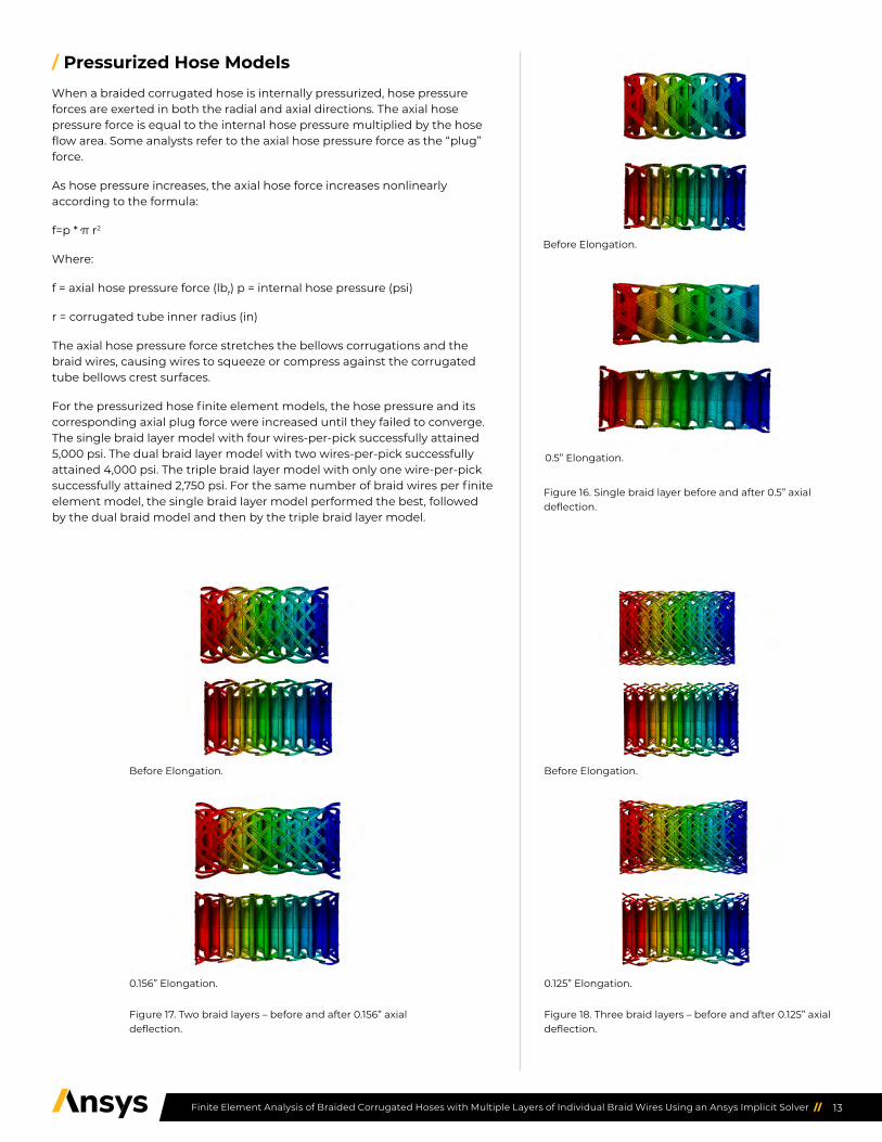
For the pressurized hose finite element models, the hose pressure and its corresponding axial plug force were increased until they failed to converge. The single braid layer model with four wires-per-pick successfully attained 5,000 psi. The dual braid layer model with two wires-per-pick successfully attained 4,000 psi. The triple braid layer model with only one wire-per-pick successfully attained 2,750 psi. For the same number of braid wires per finite element model, the single braid layer model performed the best, followed by the dual braid model and then by the triple braid layer model.

Figure 16. Single braid layer before and after 0.5” axial deflection.

Before Elongation.

0.5” Elongation.

Before Elongation.

0.156” Elongation.

Figure 17. Two braid layers – before and after 0.156” axial deflection.

Before Elongation.

0.125” Elongation.

Figure 18. Three braid layers – before and after 0.125” axial deflection.


Examination of the wire axial forces for each braid layer shows that the forces within the innermost braid layer are the highest, followed by those in the second and third braid layers.

As expected, the axial hose stiffness for pressurized hoses is much higher than for unpressurized hoses.

The maximum FEM hose pressure limits for the single, dual and triple braid layer models are tabulated in Table 10.

The next three figures show the innermost braid wires compressing against the corrugated tube crest surfaces. Notice that the tube crests expanded or bulged axially relative to the troughs.

FEM Description Single Layer Two Layers Three Layers



No. of wire-per-pick 4 2 1


Input (1) Hose internal pressure limit (psi) 5,000 4,000 2,750

Hose axial plug force (lbf) 552 442 304

Output Hose axial deflection (in) 0.083 (@ 5,000 psi) 0.159 (@ 4,000 psi) 0.078 (@ 2,750 psi)

Hose axial stiffness - pressurized (lbf/in) 6,651 (@ 5,000 psi) 2,780 (@ 4,000 psi) 3,897 (@ 2,750 psi)

Table 10. Pressurized Hose FEM Deflection Results for Single and Multiple Braid Layers (1)

(1) 316 stainless steel (42,100 psi yield stress)

Figure 19. Single Braid Layer with 4 wires per pick @ 5,000 psi (& 552 plug lbf): total deformation = 0.083”.

Figure 20. Two braid layers with 2 wires-per-pick @ 4,000 psi (& 442 psi lbf): total deformation = 0.159”.

Figure 21. Three braid layers with 1 wire-per-pick @ 2,750 psi (& 304 plug lbf): total deformation = 0.078”.


Figure 22 shows the FEM results for the pressurized hose models with one, two and three layers of braid wires. Notice that the braid wire axial forces for the multilayer braid models are substantially different for each braid layer.

Figure 22. Single layer of braid wires - 5,000 psi - FEM results.

Figure 23. Two layers of braid wires - 4,000 psi - FEM results.

Figure 24. Three layers of braid wires – 2,750 psi – FEM results.


/ Axial and Wire Tensile Forces Within Individual Braid Layers

Hand Calculations – Tensile Forces Along Braid Wire Axes

A standard method for hand calculating the forces within braid wires is to assume the entire axial hose pressure plug force is carried entirely by the braid wires and that none of the axial force is carried or transmitted through the corrugated tube bellows.

Since braid wires are not oriented in-line with the hose axis, but are instead oriented at an angle.

The helix angle is shown in Figure 25.

From Liquid Rocket Lines, Bellows, Flexible Hoses, and Filters[7] : “Multiple layers of braid may be used to achieve greater strength within wire-handling capacity of the braider and without too great a sacrifice in flexibility. Because of the difficulty in obtaining perfect load distribution between layers of braid, it is reasonable to assume that the second layer is only 80% efficient.”

Based on this assumption,

When there are two braid layers, the averaged force along each wire is assumed to be

For two braid layers, hand calculations (without performing FEA) result in an estimated average wire axial force of 14.88 lbf and an average wire tensile stress of 74,026 psi.

Ansys – Tensile Forces Along Braid Wire Axes

Note: The Ansys Axial Force (X Axis) is along the helical braid axis for each individual wire.

The Ansys axial forces for the two braid layer hose FEM pressurized at 4,000 psi are displayed in Figures 26, 27 and 28. Notice the large variation in wire forces between the inner and outer braid layers.

Figure 25. - Helix braid angle.

Figure 26. Ansys axial forces - two braid layers.

Figure 27. Ansys axial forces - outer braid layer.

Figure 28. Ansys axial forces - inner braid layer.


The highest axial forces occur at the wire tips where the braid wires are welded or bonded to the ends of the corrugated tube.

The following table shows the pressurized hose FEM results for one, two and three braid layers. The maximum FEM hose pressure was determined by pushing the models to their limits. The maximum principal stresses within the corrugated tube as well as the braid wire tensile stresses are greater than the 316 stainless steel (42,100 psi) yield stress for all of the pressurized hose FEMs. For the single braid layer FEM, the wire tensile stress approaches the ultimate tensile strength, and the corrugated tube Maximum Principal stress exceeds the ultimate tensile stress by approximately 2%.

The next table shows the variation in axial forces and braid wire tensile stresses between braid layers. Since the Ansys axial forces spike at the ends of the hose assemblies, for discussion purposes, “typical” values were obtained by taking a random sample of values from the central portion of the hose models and averaging them. The typical braid wire axial stress for the 5,000 psi single braid layer hose model was approximately 37,800 psi. For the 4,000 psi dual braid layer hose model, the typical braid wire stresses for the inner and outer braid layers were approximately 42,300 psi and 11,400 psi respectively. For the triple braid layer model with 2,750 psi, the typical braid wire axial stresses were 25,500 psi, 1,000 psi and 300 psi respectively for the inner, middle and outer braid layers. This data demonstrates the large variation of braid wire tensile stresses for hose models which contain multiple layers of braid wires.

Force along wire axis (lbf) Wire tensile stress (psi)

Ansys FEM - at wire tips 10.779(1) 53,710(1)

Hand calculation 14.88 74,026

Table 11. Wire Tensile Force and Axial Stress – Two Braid Layers – 4,000 psi Hose Pressure.(1) 316 stainless steel (42,100 psi yield stress).

No. of braid layers One Two Three

Maximum FEM hose pressure (psi) & hose plug force (lbf)

5,000 4,000 2,750

552 442 304

Reaction force (lbf) 547 445 306

Hose axial deflection (in) 0.083 0.159 0.078

Ansys Axial force (lbf) & wire tensile stress (psi) max/min

+10.657 53,000 +10.799 53,710 +6.190 30,800

-9.570 -47,600 -11.363 -56,500 -6.138 -30,500

Max. Principal Stress @ corrugated tube max/min (psi)

85,600 76,000 61,300

-32,000 -14,700 -5,100

Table 12. FEM Results – Maximum Pressurized Hose Models (1).(1) 316 stainless steel (42,100 psi yield stress & 84,100 psi ultimate tensile strength).

maximum Ansys forcealong_wire=

maximum Ansys axial stresswire=


/ Early Termination (Non-Convergence) of Deflection and Internally Pressurized Hose Finite Element Analysis Models

Hose finite element models sometimes failed to converge when high loads (forced deflection or internal hose pressure and axial plug pressure force) were applied to them. By default, the Ansys force residual tolerance and the moment residual tolerance is automatically set to 0.5%.

An analyst can graphically display Newton-Raphson residual forces by specifying the number of residual forces to display, prior to starting an analysis. If a model converges, the locations and intensities of the residual forces during the analysis will not be available for viewing. But when a model doesn’t converge, examination of the location of the residual forces can help identify why it didn’t converge.

Since the surfaces where the forced deflection load is applied is very close to the free end of the corrugated tube, this often causes localized force residual hot spots nearby.

The residual force hotspots are very shallow, penetrating only a very short distance into a mesh element. The residual force hotspots frequently occur at the extreme tips of the wire ends, within the last trough of the last corrugated tube, or at the last tube crest. Sometimes they also occur at the interface between consecutive beam elements or where beams cross.

No. of braid layers One Two Three

Max. FEM Hose pressure (psi) 5,000 4,000 2,750

Braid layer location

Ansys Axial Force (lbf)

First/Only Inner Outer Inner Middle Outer

+10.657-9.570

+10.799-8.566

+8.999-11.363

+6.190-6.138

+5.740-1.790

+4.105-4.413

Ansys Axial Force ~ typical value (lbf) +7.60 +8.50 +2.30 +5.14 +0.20 +0.06

Braid wire tensile stress ~ typical value (psi) 37,800 42,300 11,400 25,500 1,000 300

Table 13. Axial Forces and Braid Wire Tensile Stresses within Individual Braid Layers. (1)

(1) 316 stainless steel (42,100 psi yield stress)

Figure 29. Residual force hotspots at wire tip and between consecutive beam elements.

Figure 30. Residual force hotspots within corrugated tube trough.

Figure 31. Residual force hotspots at the last corrugated tube crest.Figure 32. Residual force hotspots between crossing wires.


It was hoped that by specifying a finer mesh in the zones where the Newton-Raphson residual force occurs, that those models could be pushed further. But specifying a finer mesh in those areas did not allow models to proceed further than previously.

Manually overriding and increasing the residual force and moment tolerances to 10%/5% respectively, often allowed those models to be pushed farther without sacrificing solution accuracy. A simple way to verify that changing these tolerances does not affect the accuracy of the FEM results is to compare the reaction forces with the input forces. If they match closely, this confirms that adjusting the residual tolerances did not affect the results’ accuracy.

In order to push some models even further, the residual force tolerance was intentionally turned off and the moment residual tolerance was set at 5%. After these models converged, the input and output forces were compared. Typically, this modeling technique was successful in obtaining convergence without sacrificing accuracy.

Even when the residual force tolerance is turned off and the moment residual force tolerance is set at 5%, the displacement residual tolerance is still being strictly enforced by Ansys. This combination of enforcing the displacement residual tolerance and utilizing a 5% moment residual tolerance is usually sufficient to obtain convergence of hose models while maintaining accuracy.

An additional benefit of overriding the residual force tolerance and the moment tolerance is that it reduces the number of iterations required for convergence and computer run times.

/ Sensitivity of Deflection Models Compared to Pressurized Hose ModelsBraided hose displacement models are easier for a FEA solver to analyze than pressurized hose models with an axial plug force.

When a “displacement” is applied at the unconstrained, free end of the corrugated tube, all of the tube corrugations stretch to some extent. The corrugations nearest the application of the displacement stretch the most while corrugations closer to the fixed end stretch less.

But when a force load is applied to surfaces near the free end of the corrugated tube to simulate a hose pressure plug-force, even though all the tube corrugations will eventually stretch to some degree, this concentrated plug force is basically applied locally. This concentrated force can cause convergence problems, exaggerating the residual force tolerance issue previously discussed.

When axial deflection is applied to the free end, the free end deflects directly along the hose axis. But when a hose plug (axial) force is applied it can cause the free end of the hose to wobble in 3D space as beam-to-beam and beam-to-corrugated-tube elements continuously change contact status throughout the simulation. Wobbling increases computer run time.

After a pressurized hose finite element model with a plug force converges, the axial deflection at the free end will be known. By removing the initial plug force and replacing it with the axial deflection from the previous plug force model, when this new deflection model converges, the resulting FEM reaction force will be equal to the previously applied plug force. Pressurized hose FEMs with radial pressure and deflection solve much faster than pressurized hose FEMs with radial pressure and a plug force.

/ Comments Regarding Ansys HPC PacksAs an Ansys Associate, the author had temporary access to Ansys Professional and one HPC pack which can utilize up to eight cores. The single HPC pack allowed four cores to be utilized on the author’s computer instead of two cores, reducing run times by approximately 50%. Anyone interested in analyzing braided corrugated hoses should consider purchasing at least two Ansys HPC Packs (allowing 32 computer cores to be utilized) and as much computer memory as possible, on the fastest platform available with more cores than the number allowed by the HPC pack license.

/ Selection of Dimensions for Non-Proprietary Braided Corrugated Hose ModelsThe Ansys Academic license is limited to 50 bodies, 300 faces (surfaces), 7,500 equations and 32,000 nodes/elements.

The author examined a Flexible Hose Engineering Design Guide[8] and decided to initially try creating and modeling a non-proprietary 3/8” I.D. corrugated hose with one layer of braid wires. The manufacturers’ hose guide shows that a nominal 3/8” I.D. stainless steel hose has an outside diameter of 0.590”. Using these diameters as a starting point, a U-shaped bellows profile was created using conventional drafting techniques. The author decided to keep things simple and to use fractional measurements whenever possible. A tube crest centerline-to-centerline distance of approximately 1/8” (0.120”) was chosen. In combination with a wall thickness of 0.012”, this resulted in a visually acceptable corrugated tube U-shaped profile, as shown in Figure 1.

As mentioned, a single layer of braid wires increases the outside diameter by at least four times the nominal diameter of the braid wires. Refer to Figure 5. The flexible hose design guide(8) for a single layer of braid wires specifies an outside diameter of 0.640”. Subtracting 0.590” from 0.640” and dividing by 4 gives an approximate braid wire diameter of 0.0125”. The author decided to model 1/64th (~0.016”) diameter wires instead.


The “helical length” is the axial distance which corresponds to 360° of helical rotation about the longitudinal axis. While creating the first and subsequent finite element models, a helical length of approximately 1.75” was used. This helical length corresponds with a braid angle of approximately 43°. A braided corrugated hose model with an axial length of approximately 1.75” was attempted. But this required more than 32,000 nodes and elements, exceeding the Ansys Academic license limits. Reducing the hose length to 1.2” and experimenting with mesh sizing, an acceptable model size was eventually obtained. When additional layers of braid layers were added to the model, the mesh sizing was adjusted accordingly.

/ Finite Element Analysis Results of Single Layer Corrugated Hose vs. Manufacturer’s Operating Pressure Limits

Braided corrugated hose operating and burst pressures depend on a number of factors, including the number of braid wires within a braid layer and the total number of braid layers. A thin-walled corrugated tube without any braid wires can only sustain a small amount of internal hose pressure before deforming excessively due to a combination of axial elongation and column buckling instability (squirm).

A U-shaped, corrugated tube with a 0.590” outside diameter can physically accommodate 24 picks of braid wires with five 0.016” diameter braid-wires-per-pick. For this hose size, there is room for 120 braid wires per braid layer. But due to Ansys Academic license restrictions, only 48 wires could be included within the finite element models.

As mentioned, analyzing a pressurized hose is more difficult than analyzing non-pressurized axial hose elongation. So the real test for a finite element analysis solver is how well it can analyze a pressurized braided corrugated hose model. Since the manufacturer’s “normal burst pressure” is listed as 5,800 psi, different modeling parameters and techniques were implemented to see how far an Ansys implicit analysis could be pushed while striving to attain 5,800 psi.

It is important to keep in mind that the Ansys Academic finite element models only contain 40% of the full complement of braid wires on a nominal 3/8” I.D. commercial hose with one layer of braid wires. Even with this reduced number of braid wires, the Ansys Academic single braid layer hose finite element analysis model successfully attains 5,000 psi before 1) either the wires pass through the corrugated tube wall thickness or 2) the corrugated tube mesh collapses or implodes or 3) the analysis stops because the Ansys residual forces/moments are exceeded.

The following table lists the manufacturer’s[8] maximum working pressure, maximum test pressure and burst pressure for a nominal 3/8” I.D. braided stainless steel corrugated hose with a single layer of 120 stainless steel braid wires. (24 picks x 5 wires-per-pick = 120 wires.)

A commercial nominal 3/8” I.D. corrugated tube is rated at 80 psi. Adding a single braid layer increases the maximum working pressure to 1,450 psi. This increases the maximum working pressure by a factor of 18:1.

The maximum working pressure specification for a commercially rated corrugated hose with 120 braid wires is 1,450 psi[8]. Therefore, while performing finite element analysis, the FEA solver would need to be able to attain 1,450 psi without braid wires passing through the corrugated tube or braid wires passing through other wires.

For the finite element analysis model with a single layer of 48 braid wires, the Ansys implicit solver attained 5,000 psi without any wire penetration issues. (5,000 psi is 3.4 times the 1,450 psi “maximum working pressure” specification).

Hose I.D. Hose O.D. Total No. of Braid Wires

Maximum Working

Pressure (psi)

Maximum Test Pressure

(psi)

Maximum FEM Pressure

Limit (psi)

Burst Pressure (psi)

Hose engineering

guide[8]

0.375 0.59 0 80 120 N/A -

0.64 (120) 1,450 2,175 N/A 5,800

FEM - 1 braid layer

0.375 0.654 48 N/A N/A 5,000 N/A

Table 14. Engineering Guide Max. Working Pressure Comparison with Max. Pressure FEA Results.T316L stainless steel (42,100 psi yield stress).[8]


Even though not a direct comparison (48 wires vs. 120 braid wires), this demonstrates that the Ansys implicit solver is capable of analyzing a commercial braided corrugated hose with a nominal 3/8” I.D. and one layer of (48) braid wires.

The axial deformation and hose pressure limits for finite element models with one, two and three layers of braid wires is summarized in Table 15.

/ Mesh Quality DiscussionQuadratic mesh elements are less sensitive to element distortion than linear elements. Quadratic elements represent curved edges and surfaces more accurately and are less sensitive to element distortion than linear elements. Quadratic elements allow mid-side nodes to be turned on or off by the analyst.

Since the corrugated tube crest and trough geometries have curved edges and surfaces, a higher level of modeling accuracy could possibly be attained by using quadratic elements with mid-side nodes instead of using linear elements.

Due to Ansys Academic software license restrictions (32,000 nodes maximum), linear mesh elements were used for the corrugated tube mesh and the mid-side node analysis option was turned off. One advantage of turning the mid-side nodes off is that it reduces the computer time required for analysis. Using linear elements instead of quadratic elements also reduces computer run time. It is possible that the modeling limit of 5,000 psi hose pressure could possibly be pushed further by increasing the number of mesh elements within the corrugated tube and by using quadratic elements with the mid-side node option turned on, but doing so could increase analysis time.

Figure 33. Braid weave densities with 48 and 120 braid wires per layer.

FEM Description One Braid Layer Two Braid Layers Three Braid Layers



Wires-per-pick 4 2 1


Input [1] Hose pressure limit (psi) 5,000 4,000 2,750

Output Total deformation (in) 0.083 0.159 0.078

Input [2] Hose elongation limits (in) 0.50+ 0.156 0.125

Table 15. Summary of FEM Hose Pressure and Axial Deflection Limits.(1) stainless steel @ 42,100 psi yield stress(2) stainless steel @ 30,458 psi yield stress


/ Tri-Axial Deflection FEM ResultsA single braid layer model was evaluated to test Ansys’s robustness for handling multi-axis braided corrugated hose deflection. The tri-axial Ansys hose FEM successfully converged without excessive wire penetration.

/ Severe Tip Deflection – FEM ResultsA single braid layer model (stainless steel @30,485 psi yield stress) was analyzed to test Ansys’s robustness for handling severe tip deflection. The free end of the hose was deflected 0.188” vertically downward. The FEM successfully converged without excessive wire penetration.

Figure 36 shows the corrugated tube maximum principal stress and the corrugated tube deformation resulting from a large vertical tip displacement.

Next, Figure 37 shows the braid wires flexing. This level of detail would not be possible if picks of wires had been modeled as ribbons with composite material properties.

/ Ansys FEM Discussion and ConclusionsAnsys implicit software successfully analyzes braided corrugated hoses with multiple layers of individual braid wires where each wire is modeled as an individual component or structure. As the hose simulation progresses, each braid wire slides, stretches and flexes, changing back-and-forth between contact and non-contact. This is an extremely complex and challenging contact modeling simulation. The Ansys finite element model results are extremely detailed, providing insight into the underlying physics of how internally pressurized braided corrugated hose components stretch and deform. A summary of the modeling highlights is listed below.

1. Axial hose deflection FEMs - Single, dual and triple braid layer finite element analysis models successfully sustained large axial deflection. The single braid layer hose model stretched into the elastic-plastic material properties range.

2. Tri-axial hose deflection FEM - A single braid layer finite element analysis model successfully sustained large tri-axial deflection.

3. Tip deflection FEM - A single braid layer finite element analysis model successfully sustained large tip deflection.

4. Pressurized hose FEMs - Single, dual and triple braid layer pressurized hose finite element analysis models successfully converged. All of these models progressed far into the elastic-plastic material properties range. For the single braid layer FEM, the braid wire tensile stresses were elastic-plastic and the corrugated tube stresses exceeded the ultimate tensile strength by approximately 2%. Even though the single braid layer finite element hose model contains only 40% of the full complement of braid wires used on a commercial braided corrugated hose with a 3/8” I.D. hose and one layer of braid wires, the Ansys model successfully attained 5,000 psi, which is 3.4 times the hose manufacturer’s rated maximum working pressure specification.

Description (in)

FEM Input FEM Output[1]

Delta X Delta Y Delta Z Total

-0.093 -0.093 0.250 0.286

Table 16. Deflection along X, Y and Z axes.(1) stainless steel @ 30,458 psi yield stress.

Figure 34. Tri-axial deflection - single braid layer - front and side views.

Figure 35. Vertical tip deflection - single braid layer - front and side views.

Figure 36. Severe tip deflection FEM – single braid layer – maximum principal stress.

Figure 37. Individual braid wires flexing – vertical tip deflection FEM.


Any and all ANSYS, Inc. brand, product, service and feature names, logos and slogans are registered trademarks or trademarks of ANSYS, Inc. or its subsidiaries in the United States or other countries. All other brand, product, service and feature names or trademarks are the property of their respective owners.

ANSYS, Inc. Southpointe

2600 Ansys Drive Canonsburg, PA 15317

U.S.A. 724.746.3304

[email protected]

© 2021 ANSYS, Inc. All Rights Reserved.

If you’ve ever seen a rocket launch, flown on an airplane, driven a car, used a computer, touched a mobile device, crossed a bridge or put on wearable technology, chances are you’ve used a product where Ansys software played a critical role in its creation. Ansys is the global leader in engineering simulation. We help the world’s most innovative companies deliver radically better products to their customers. By offering the best and broadest portfolio of engineering simulation software, we help them solve the most complex design challenges and engineer products limited only by imagination.

Visit www.ansys.com for more information.

23

Important Findings

a. At high pressure, the corrugated tube crests deflect or bulge substantially in the axial direction compared to the tube troughs.

b. The innermost braid layer carries a substantially larger portion of the total braid wire axial forces than outlying braid layers. There is also a wide variation of wire tensile forces within any braid layer.

This white paper demonstrates Ansys implicit software is robust for analyzing braided metallic corrugated hoses with multiple layers of individual metallic braid wires.

/ About the AuthorMichael McCain is a Professional Engineer with Bachelor of Science in Mechanical Engineering (BSME) and Master of Mechanical and Aerospace Engineering (MMAE) degrees from the Illinois Institute of Technology. He has completed numerous master level and post-graduate courses including linear and nonlinear finite element analysis, experimental stress analysis and software development. Mr. McCain specializes in structural contact finite element analysis and mathematical modeling. He has over 20 years of professional FEA/FEM experience and can be contacted at [email protected] or https://www.linkedin.com/in/michael-mccain-PE/

/ References1. Laupa AA, Weil NA. Analysis of U-Shaped Expansion Joints. ASME. J. Appl. Mech. 1962; 29(1):115-123. doi:10.1115/1.3636442.

2. Pierce, and Stephen O. “Failure Analysis of Braided U-Shaped Metal Bellows Flexible Hoses.” Thesis, 2010 – UMI Number: 1487677

3. Rial, D. , Tiar, A. , Hocine, K. , Roelandt, J. and Wintrebert, E. (2015), Metallic Braided Structures: The Mechanical Modeling. Adv. Eng. Mater., 17: 893-904. 10.1002 adem.201400422

4. Otin, Ruben, and Roger Isanta. A CAD Tool for the Electromagnetic Modeling of Braided Wire Shields . CIMNE – International Center for Numerical Methods in Engineering. http://tts.cimne.com/ermes/documentacionrotin/TechReport-CADZt.pdf

5. Otin, Ruben, and Jaco Verpoorte. A Finite Element Tool for the Electromagnetic Analysis of Braided Corrugated Shields. CIMNE – International Center for Numerical Methods in Engineering http:/. /tts.cimne.com/ermes/documentacionrotin/PrePrint-BWS-Zt-Tool.pdf

6. Vectors in Three Dimensional Geometry http://www.ignou.ac.in/upload/UNIT%203%20THREE%20DIMENNSIONAL%20FINAL-BSC- 012-BL4.pdf

7. Liquid Rocket Lines, Bellows, Flexible Hoses, and Filters – NASA-SP-8123; April 1, 1977; page 90 https://ntrs.nasa.gov/search.jsp?R=19780008146

8. US Hose Corporation – Engineering Guide No. 350 – 8th Edition – Flexible Metallic Hose, Braid and Assemblies – 2013 – Pages 6 and 7 http://www.fsrs.com/images/pdf/us-hose-metal-type.pdf

finite element analysis of braided corrugated hoses with

Documents