Finite Element Analysis for EngineersBasics and Prac cal Applica ons with Z88Aurora

Frank RiegReinhard HackenschmidtBe na Alber-Laukant

Book ISBN978-1-56990-487-9

HANSER Hanser Publishers, Munich • Hanser Publica ons, Cincinna

Preface, Contents, Sample Pages

Following the ongoing strong demand in the last years for an English version of the German standard work “Finite Elemente Analyse für Ingenieure” we decided to satisfy this.Our aim with this book is:To provide well-chosen aspects of the finite elements for a student of engineering sciences from the 3rd semester and an engineer already established in the job in such a way that he can apply this knowledge immediately to the solution of practical problems.Therefore, already in the title of the book we speak of finite element analysis (FEA) and not of finite element method. This gigantic field has left behind the quite dubious air of a method for a long time and today is the engineer’s tool to analyse structures. Of course, one can do much more with this process than mechanics: heat flows, electric fields and magnetic fields, actually, differential equations and boundary problems for different fields in general – all of this can be solved with it.However, everything has begun with the calculation of mechanical structures and, hence, we want to limit ourselves in this book to linear and non-linear statics, stationary heat conduction and natural frequencies. The engineer’s aspect is very substantial to us – it does not appear in the title of this book without any reason: The process was developed fairly “intuitively” in the fifties by airplane engineers for static calculations of airplane structures. It is a process from engineers for engineers!Hence, we proceed as follows: After a really easy demonstration of the basic procedure, we will discuss the most important points of the elasticity theory, the engineering mechanics and the thermodynamics, as far as the FEA is concerned. With this knowledge we continue with the derivation of the element stiffness matrices. This theoretical knowledge is indispensable for proper and clever working with FEA programs. Then we look at the compilation procedure, at the storage processes and at the solving of the equation systems to calculate the unknowns.In order to transfer your knowledge into practice, we have put two FE programs on DVD: Z88®, the open source finite elements program for static calculations, programmed by the lead author of this book, as well as Z88Aurora®, the very comfortable to use and much more powerful free-ware finite elements program which can also be used for non-linear calculations, stationary heat flows and natural frequencies. Both are full versions with which arbitrarily big structures can be computed. The only limits are given by your computer concerning main storage and disc storage and by your powers of imagination. Z88 and Z88Aurora are ready-to-run for Windows,

Preface

vi  Preface 

LINUX, as well as for Mac OS X. For Z88 we directly provide the sources, so that you can study the theoretical aspects in the program code and extend it if necessary. This way, you can also understand the working of memory processes, equations solvers and so forth. Z88 is transpar-ent for the user through input and output via text files. It is a FEA program in the quite classical and original sense. In addition, we think: You only learn the basics with a program like this, as every numerical value can and has to be controlled. As soon as you have understood the basic procedure, you can work with Z88Aurora, which was developed at our Chair of Engineering De-sign and CAD at the University of Bayreuth, Germany, with promotion of the Oberfrankenstif-tung. Z88Aurora does not take second place in look and feel compared to the commercial FEA programs and allows a very professional and contemporary work, directly from CAD data. We do not refer to the known commercial FEA programs here because the versions that are free of charge only offer very limited options concerning the structure sizes with which you could not compute several of the following examples at all. Moreover, we cannot offer source codes for them. In later sections of the book there are many practical examples that we recommend to check. The DVD also contains the input files for all examples. The examples are selected in a way that gradually explains the different aspects of the calculation of structures and mechani-cal structures.Furthermore, we have developed an app for Android devices called Z88Tina (www.z88tina.de) which is a very, very small cousin of our full-featured freeware FEA program Z88Aurora (www.z88.de) and is derived from the open source FEA program Z88V14OS. Z88Tina can be dow-loaded from Google Play Store: https://play.google.com/store/apps/details?id=z88tina.frFor this fourth German edition (and first English edition) we have completely revised our book on finite element analysis: The theoretical section has been extended concerning shell elements (by Prof. F. Rieg, PhD), non-linear calculations (by C. Wehmann, PhD), stationary heat conduc-tion (by M. Frisch, M.Sc.) and natural frequencies (by M. Neidnicht, PhD). The examples have been strongly extended and updated. Our employees M. Frisch, M.Sc., M. Neidnicht, PhD, F. Nützel, M.Sc., C. Wehmann, PhD, J. Zapf, PhD, and M. Zimmermann, M.Sc., did the program-ming and testing of Z88Aurora version 2 and gave valuable recommendations for the text of this book. We wish to thank them all a lot. Our very special thanks is directed towards Kevin Deese and Christoph Wehmann for their systematic translation error search. It was a hell of a work. We also thank our publishing house Carl Hanser Verlag for the exemplary realization of this book.The work on this book was again a pleasure to us and we hope you will enjoy this book.

Frank Rieg, Reinhard Hackenschmidt and Bettina Alber-LaukantBayreuth, Germany, June 2014

Preface ................................................................................................ v

1 Introduction  ....................................................................................... 1

2 The Basic Procedure  .......................................................................... 5

3 Some Elasticity Theory  ..................................................................... 233.1 Displacements and Strains  ............................................................................................ 23

3.1.1 For the Truss  ............................................................................................ 233.1.2 For Plane Stress  ........................................................................................ 253.1.3 In Space  .................................................................................................... 313.1.4 For the Plate  ............................................................................................. 32

3.2 Stress-Strain Relations  ................................................................................................... 343.3 Basics of Thermomechanical Loading  ......................................................................... 443.4 Basic Principles of Natural Vibration  .......................................................................... 473.5 Basic Principles of Non-linear Calculations  ............................................................... 50

4 Finite Elements and Element Matrices  ............................................ 634.1 Basics of Element Stiffness Matrices  ........................................................................... 654.2 Constitutive Matrices  ..................................................................................................... 694.3 B Matrix  ............................................................................................................................ 704.4 Shape Functions  .............................................................................................................. 714.5 Integration  ....................................................................................................................... 814.6 The Application of Loads, Load Vectors  ...................................................................... 88

4.6.1 The Basic Procedure  ................................................................................. 884.6.2 Plate Elements  .......................................................................................... 914.6.3 Volume Elements ...................................................................................... 934.6.4 Plane and Axial-Symmetrical State of Stress  ........................................... 1044.6.5 Distributed Loads for Beams  .................................................................... 1064.6.6 Gerber Joints for Beams  ........................................................................... 108

4.7 A complete Element Stiffness Routine  ........................................................................ 112

Contents

viii  Contents

4.8 Some Remarks on Modelling  ............................................................................ 1214.8.1 Choice of Element Types  ..................................................................... 1214.8.2 Polymers and Material Laws  ............................................................... 1294.8.3 Structural Optimization  ...................................................................... 130

4.9 Some Remarks on Shells  ................................................................................... 1344.10 Element Matrices for Heat Transfer  ................................................................. 1484.11 Element Matrices for Vibration  ........................................................................ 1504.12 Element Matrices of the Non-linear Finite Element Analysis  .......................... 152

5 Compilation, Storage Schemes and Boundary Conditions  ......... 1635.1 Compilation  ....................................................................................................... 1635.2 Storage Schemes  ............................................................................................... 174

5.2.1 Band Width Storage Scheme  ............................................................... 1765.2.2 The Skyline Storage Scheme  ............................................................... 1805.2.3 The Jennings Storage Scheme  ............................................................. 1825.2.4 The Non-Zero Storage Scheme  ............................................................ 1905.2.5 Summary of the Storage Schemes  ...................................................... 196

5.3 Boundary Conditions  ........................................................................................ 1975.3.1 Single Forces and Single Displacements  ............................................ 1975.3.2 Distributed Loads with Plates  ............................................................. 2005.3.3 Fixture of plates  .................................................................................. 2025.3.4 Boundary Conditions in Temperature Analyses  ................................. 2035.3.5 Boundary Conditions with Vibration  .................................................. 2065.3.6 Boundary Conditions in the Non-linear Finite Element Analysis  ...... 207

6 Solvers  ............................................................................................. 2096.1 Direct Solvers  .................................................................................................... 210

6.1.1 The Cholesky Solver  ........................................................................... 2126.2 Condition and Scaling  ....................................................................................... 2146.3 Iterative Solvers  ................................................................................................ 223

6.3.1 The Jacobi Method  .............................................................................. 2256.3.2 The Gauss-Seidel Method  .................................................................... 2266.3.3 The SOR Method and the JOR Method  ................................................ 2266.3.4 The basic CG Solver  ............................................................................ 2276.3.5 The CG Solver with Pre-conditioning  .................................................. 229

6.4 Solver for Thermomechanical Problems  ........................................................... 2446.5 Solver for Vibration Problems  ........................................................................... 2446.6 Solver for the Non-linear Finite Element Analysis  ........................................... 254

7 Stresses and Nodal Forces  ............................................................ 2577.1 Stresses  ............................................................................................................. 2577.2 Reduced Stresses  .............................................................................................. 2647.3 Nodal Forces  ...................................................................................................... 271

Contents  ix

8 Mesh Generation of Curvilinear Finite Elements  ......................... 2758.1 Basis Considerations of the Procedure  ............................................................. 2758.2 Mathematical Foundations  ............................................................................... 2778.3 Description of a Simple Mapped Mesher  .......................................................... 281

9 Z88: The Basics  ............................................................................... 2899.1 General Information  .......................................................................................... 289

9.1.1 Summary of the Z88 Element Library  ................................................ 2909.2 The Open Source FE Program Z88  .................................................................... 302

9.2.1 Overview of the Z88 Program Modules  .............................................. 3029.2.2 Dynamic Memory Z88  ........................................................................ 3059.2.3 The Input and Output of Z88:  ............................................................. 308

9.3 The Freeware FE Program Z88Aurora  .............................................................. 3129.3.1 Overview of the Z88Aurora Modules  .................................................. 3129.3.2 Memory Requirement in Z88Aurora  .................................................. 3159.3.3 The Input and Output of Z88Aurora  ................................................... 316

10 Z88: The Modules  ........................................................................... 31910.1 The Linear Solver Z88R ..................................................................................... 319

10.1.1 Z88R: The Cholesky Solver  ................................................................. 32010.1.2 Z88R: The Sparse Matrix Solvers SICCG and SORCG  ........................ 32110.1.3 Z88R: The Sparse Matrix multi-core Solver PARDISO  ........................ 32310.1.4 Which Solver to choose? ...................................................................... 32410.1.5 Explanations for Stress Calculations  .................................................. 32410.1.6 Explanations for Nodal Force Calculations  ......................................... 325

10.2 The Mapped Mesher Z88N  ................................................................................ 32510.3 The Advanced Mapped Mesher in Z88Aurora  .................................................. 328

10.3.1 The Use of Z88N in Z88Aurora  ........................................................... 32810.3.2 Tetrahedron Refiner Z88MTV  ............................................................. 32910.3.3 The 2D Shell Thickener Z88MVS  ........................................................ 331

10.4 The OpenGL Plot Program Z88O in Z88 V14 OS or the Post-Processor of Z88Aurora  ..................................................................................................... 331

10.5 The DXF Converter Z88X  .................................................................................. 33510.6 The 3D Converter Z88G  .................................................................................... 34410.7 The Ansys Converter Z88ASY in Z88Aurora  .................................................... 34710.8 The Abaqus Converter Z88INP in Z88Aurora  .................................................. 34910.9 Das Cuthill-McKee Program Z88H  .................................................................... 35010.10 The STEP Import Z88GEOCON (STEP) in Z88Aurora  ....................................... 35210.11 The STL Converter Z88GEOCON (STL) in Z88Aurora  ....................................... 35410.12 The Tetrahedron Mesher in Z88Aurora  ............................................................ 35510.13 The Picking Module of Z88Aurora  .................................................................... 35610.14 The Material Data Base of Z88Aurora  ............................................................... 35810.15 Applying Boundary Conditions in Z88Aurora  .................................................. 358

x  Contents

10.16 The User Support with Spider in Z88Aurora  .................................................... 35910.17 The Thermomechanical Solver in Z88Aurora  ................................................... 36010.18 The free Vibration Solver in Z88Aurora  ........................................................... 36310.19 The Non-linear Solver Z88NL of Z88Aurora  ..................................................... 366

11 Generating Input Files  .................................................................... 37111.1 General Information  .......................................................................................... 37111.2 General Structure Data File Z88I1.TXT  ............................................................ 37311.3 Boundary Condition File Z88I2.TXT  ................................................................. 37411.4 Surface and Pressure Loads File Z88I5.TXT  ..................................................... 37711.5 Material Parameters File Z88MAT.TXT  ............................................................ 38211.6 Material Data File *.TXT  ................................................................................... 38311.7 Element Parameters File Z88ELP.TXT  .............................................................. 38311.8 Integration Order File Z88INT.TXT  ................................................................... 38511.9 Mapped Mesher Input File Z88NI.TXT  ............................................................. 38611.10 Solver Parameters File Z88MAN.TXT  ............................................................... 39011.11 Comparison of the different Z88 Data File Formats  ......................................... 393

12 The Finite Elements of Z88 and Z88Aurora  .................................. 39512.1 Hexahedron No. 1 with 8 Nodes  ........................................................................ 39512.2 Beam No. 2 with 2 Nodes in Space  .................................................................... 39812.3 Plane Stress Element No. 3 with 6 Nodes  ......................................................... 40012.4 Truss No. 4 in Space  .......................................................................................... 40112.5 Shaft No. 5 with 2 Nodes  ................................................................................... 40212.6 Torus No. 6 with 3 Nodes  .................................................................................. 40412.7 Plane Stress Element No. 7 with 8 Nodes  ......................................................... 40512.8 Torus No. 8 with 8 Nodes  .................................................................................. 40712.9 Truss No. 9 in the Plane .................................................................................... 40912.10 Hexahedron No. 10 with 20 Nodes  .................................................................... 41112.11 Plane Stress Element No. 11 with 12 Nodes  ..................................................... 41412.12 Torus No. 12 with 12 Nodes  .............................................................................. 41612.13 Beam No. 13 in the Plane  .................................................................................. 41812.14 Plane Stress Element No. 14 with 6 Nodes  ....................................................... 41912.15 Torus No. 15 with 6 Nodes  ................................................................................ 42112.16 Tetrahedron No. 16 with 10 Nodes  .................................................................... 42412.17 Tetrahedron No. 17 with 4 Nodes  ...................................................................... 42712.18 Plate No. 18 with 6 Nodes  ................................................................................. 42912.19 Plate No. 19 with 16 Nodes  ............................................................................... 43112.20 Plate No. 20 with 8 Nodes  ................................................................................. 43412.21 Shell No. 21 with 16 Nodes  ............................................................................... 43612.22 Shell No. 22 with 12 Nodes  ............................................................................... 43812.23 Shell No. 23 with 8 Nodes  ................................................................................. 440

Contents  xi

12.24 Shell No. 24 with 6 Nodes  ................................................................................. 44212.25 Element/Solver Overview Z88Aurora V2  ......................................................... 444

13 Examples  ......................................................................................... 44513.1 Flat Wrench (Plate No. 7) ................................................................................... 452

13.1.1 With Z88 V14  ...................................................................................... 45313.1.2 With Z88Aurora V2  ............................................................................ 461

13.2 Crane Girder made of Trusses No. 4  ................................................................. 47113.2.1 With Z88 V14  ...................................................................................... 47213.2.2 With Z88Aurora V2  ............................................................................ 477

13.3 Gear Shaft with Shaft No. 5  ............................................................................... 48213.3.1 With Z88 V14  ...................................................................................... 48413.3.2 With Z88Aurora V2  ............................................................................ 487

13.4 Bending Girder with Beam No. 13 ..................................................................... 49113.4.1 With Z88 V14  ...................................................................................... 49213.4.2 With Z88Aurora V2  ............................................................................ 496

13.5 Plate Segment of Hexahedrons No. 1 and No. 10  .............................................. 50013.5.1 With Z88 V14  ...................................................................................... 50113.5.2 With Z88Aurora V2  ............................................................................ 507

13.6 Pipe under Internal Pressure, Plain Stress Element No. 7  ................................ 51013.6.1 With Z88 V14  ...................................................................................... 51113.6.2 With Z88Aurora V2  ............................................................................ 518

13.7 Pipe under Internal Pressure, Torus No. 8  ........................................................ 52013.7.1 With Z88 V14  ...................................................................................... 52113.7.2 With Z88Aurora V2  ............................................................................ 527

13.8 Two-Stroke Engine Piston  ................................................................................. 52913.8.1 With Z88 V14  ...................................................................................... 53013.8.2 With Z88Aurora V2  ............................................................................ 534

13.9 RINGSPANN Spring and Belleville Spring  ........................................................ 53913.9.1 With Z88 V14  ...................................................................................... 54113.9.2 With Z88Aurora V2  ............................................................................ 544

13.10 Liquid Gas Tank  ................................................................................................ 54613.10.1 With Z88 V14  ...................................................................................... 54613.10.2 With Z88Aurora V2  ............................................................................ 550

13.11 Motorcycle Crankshaft  ...................................................................................... 55213.11.1 With Z88 V14  ...................................................................................... 55413.11.2 With Z88Aurora V2  ............................................................................ 559

13.12 Torque-measuring hub  ...................................................................................... 56313.12.1 With Z88 V14  ...................................................................................... 56413.12.2 With Z88Aurora V2  ............................................................................ 565

13.13 Plane Frameworks  ............................................................................................ 56613.13.1 With Z88 V14  ...................................................................................... 56713.13.2 With Z88Aurora V2  ............................................................................ 587

xii  Contents

13.14 Gearwheel  ......................................................................................................... 58913.14.1 With Z88 V14  ...................................................................................... 59013.14.2 With Z88AuroraV2  ............................................................................. 595

13.15 3D Wrench  ........................................................................................................ 59913.15.1 With Z88 V14  ...................................................................................... 59913.15.2 with Z88Aurora V2  ............................................................................. 611

13.16 Force Measuring Element, Plane Stress Elements No. 7  ................................... 61313.16.1 With Z88 V14  ...................................................................................... 61313.16.2 With Z88Aurora V2  ............................................................................ 623

13.17 Circular Plate, Plates No. 20  .............................................................................. 62413.17.1 With Z88 V14  ...................................................................................... 62613.17.2 With Z88Aurora V2  ............................................................................ 630

13.18 Rectangular Plate with 16 Nodes Plates No. 19  ................................................ 63113.18.1 With Z88 V14  ...................................................................................... 63113.18.2 With Z88Aurora V2  ............................................................................ 638

13.19 Four-stroke Engine Pistons with Tetrahedrons No. 16  ...................................... 63913.19.1 With Z88 V14  ...................................................................................... 64013.19.2 With Z88Aurora V2  ............................................................................ 644

13.20 Motorcar Fan Wheel  .......................................................................................... 64713.20.1 With Z88 V14  ...................................................................................... 64913.20.2 With Z88Aurora V2  ............................................................................ 650

13.21 Diesel Piston  ..................................................................................................... 65313.21.1 With Z88 V14  ...................................................................................... 65413.21.2 With Z88Aurora V2  ............................................................................ 656

13.22 Calculation of a Stress Concentration Factor  .................................................... 65713.22.1 With Z88 V14  ...................................................................................... 65813.22.2 With Z88Aurora V2  ............................................................................ 663

13.23 Gear Root Stress  ................................................................................................ 66413.23.1 With Z88 V14  ...................................................................................... 66613.23.2 With Z88Aurora V2  ............................................................................ 668

13.24 Square Pipe, Shell No. 24  .................................................................................. 67013.24.1 With Z88 V14  ...................................................................................... 67113.24.2 With Z88Aurora V2  ............................................................................ 673

13.25 Submarine made of Shells No. 22  ..................................................................... 67713.26 Gear Wheel out of Tetrahedrons No. 17  ............................................................ 68213.27 Oscillating Drum  ............................................................................................... 68513.28 Modal Analysis Crankshaft  ............................................................................... 68913.29 Thermo-mechanical Analysis of a Spoon  .......................................................... 69213.30 Thermal Analysis of a four-stroke Engine Piston .............................................. 69813.31 Non-linear Calculation of a Belleville Spring  .................................................... 70213.32 Non-linear Calculation of a Hinge  ..................................................................... 706

References and further reading  .................................................... 711Index  ................................................................................................ 717

Contents  xiii

The DVD that comes with the book Finite Element Analysis for Engineers contains the program versions Z88 V14 OS and Z88Aurora V2 including all data necessary to use the examples of both versions. The content of the DVD is organized as follows:/z88_examples_z88aurora/: Examples for Z88Aurora V2/z88_examples_z88v14os/: Examples for Z88 V14 OS/z88aurora/: Installer and documentation Z88Aurora V2/z88v14os/: Unzipped directories Z88 V14 OS

Installation of Z88 V14 OSZ88 V14 OS is available as a ready-to-run version as well as a version for self-compiling in the directory /z88v14os/ for the following operating systems: � 32 BIT Windows � 64 BIT Windows � 32 BIT LINUX � 64 BIT LINUX � 64 BIT Mac OS X

In the file z88mane.pdf in the directory /z88v14os/docu/ you find the detailed documentation for installation and compiling.

Installation of Z88Aurora V2Z88Aurora V2 is available in the directory /z88aurora/ as installer for � 32 BIT Windows and � 64 BIT Windows

and as TAR.GZ for � 64 BIT LINUX Suse 12.1 and 12.2 � 64 BIT LINUX Ubuntu 11.04, 12.04 and 14.04 � 64 BIT Mac OS X ex 10.6 (Please note that when using UNIX und Mac the access rights have to be adapted.)

In the directory /z88aurora/installer/ you find the detailed installation manual for the corres-ponding operation system.Please note, that when using Mac OS X the GTK+-package gtk+4z88.dmg (which you find in the directory /z88aurora/installer/macosx) has to be installed at first.In the directory /z88aurora/docu/ you find the theory manual and the user guide.

Software UpdatesThe DVD’s software status is June 10th, 2014.On www.z88.de you can find the user forum as well as updates and error corrections.

3■■ 3.1 Displacements and Strains

3.1.1 For the Truss

When looking into books on technical mechanics or FEA we often find the following:

εx =∂u∂x

This is often accompanied by the remark “as one sees immediately”. We never considered such equations as “immediately reasonable”; hence, the derivation of the so-called relation of defor-mation and displacement is here presented in detail. It is the basis for understanding the con-tinuum elements of FEA. With this, we lean upon the excellent book of Bickford /10/, but we also recommend the lecture of Love /8/, Timoshenko /9/ and Schnell/Gross/Hauger /90/.We act on the assumption of a simple rubber band (which of course could also be a steel tape) and pull it with a force F. The origin length of the rubber band is ℓ0, the stretched tape has the length ℓ1. The extension of the tape is called Δℓ.

Figure 3.1–1: Length change of a rod by the force effect

We define the strain ε =∆ℓℓ0

with ∆ℓ = ℓ1⊆ℓ0ε =ℓ1 − ℓ0

ℓ0=

∆ℓℓ0

and ε =ℓ1 − ℓ0

ℓ0=

∆ℓℓ0 .

Some Elasticity Theory

24  3 Some Elasticity Theory

To examine the strain in every point, we select two points A and B on the tape, which are lo-cated very closely together, and call it the distance Δx.

Figure 3.1-2: Selective consideration of the displacements u in A and B

According to the definition ε =∆ℓℓ

=ℓ1 − ℓ0

ℓ0.

By implication, the strain in A0 is

εx (A0) = limA0B0→0

A1B1 − A0B0

A0B0

with A1B1 representing the distance between A1 and B1 resp. A0B0 representing the distance between A0 and B0.With A0B0 = Δx and

A1B1 = (x + ∆x + u(B0)) − (x + u(A0)) = ∆x + u(B0) − u(A0)

is

εx (A0) = limA0B0→0

A1B1 − A0B0

A0B0= lim

A0B0→0

∆x + u(B0) − u(A0) − ∆x∆x

We can call the difference u(B0) – u(A0) Δu and get:

εx (A0) = limA0B0→0

∆x + ∆u + ∆x∆x

= limA0B0→0

∆u∆x

lim∆x→0

∆u∆x

and in the limiting process:

εx(A0) =dudx

in A0

or in general:

ε = u’ “Strain-deflection function”

This means: The strain (or expansion) ε is the derivation of the deflection function u(x). Thus

εx = u’ =dudx

4.8 Some Remarks on Modelling  121

}

b[180 + k3-2]= b[60 + k3-1];

b[180 + k3-1]= b[ k3-2];

b[240 + k3-1]= b[120+ k3 ];

b[240 + k3 ]= b[60 + k3-1];

b[300 + k3-2]= b[120 +k3 ];

b[300 + k3 ]= b[ k3-2];

}

return(0);

}

If you want to get to the bottom of the program-technical conversions with the help of the pro-gram Z88, please note the C-routines according to Table 4.7-1.

Table 4.7-1: C-routines for continuum elements

Element type Element stiffness Element load vector Stress routine20 nodes hexahedron HEXA88.C BHEXA88.C SHEX88.C8 nodes hexahedron LQUA88.C BLQUA88:C SLQU88.C6 and 8 nodes plane stress element/torus

QSHE88.C BQSHE88.C SQSH88.C

12 nodes plane stress ele-ment/torus

CSHE88.C BCSHE88.C SCSH88.C

6 nodes plate SPLA88.C BSPLA88.C SSPL88.C8 nodes plate APLA88.C BAPLA88.C SAPL88.C16 nodes plate HPLA88.C BHPLA88.C SHPL88.C10 nodes tetrahedron TETR88.C BTETR88.C STET88.C4 nodes tetrahedron SPUR88.C BSPUR88.C SSPU88.C

■■ 4.8 Some Remarks on Modelling

4.8.1 Choice of Element Types

How to transform a real structure into a finite element model? One possible answer to this sim-ple sounding, but extremely complicated question, you will find in chapter 13 with different examples. However, let us start reflecting some basic thoughts:

122  4 Finite Elements and Element Matrices

Since Kopernikus and Galilei we know that the world is a sphere, a 3D item and no plane stress element. The plane stress element, however, is a typical 2D item. All real components are al-ways 3D items, so only with 3D CAD programs parts can be described really close to reality. Please keep in mind that a 2D drawing, no matter whether generated on a drawing board or in a 2D paint program, in reality only is an aggregation of drawing conventions. As a former de-signer’s colleague of us used to say: “It is crazy! First of all, we have to flatten a real component in our head to transfer it into a drawing. Then the viewer of the drawing must rebuild the com-ponent in his head!”Thus a part of the answer is already given: A real part can always and principally be illustrated by volume elements. This action has only one flaw: It just makes the highest demands on calcu-lation power, main memory and disk storage. But the trend is towards this direction, and a new generation of the FE programs, which are especially intended for the designers, so to speak “for the small FE calculation in between”, only operate with volume elements or shell elements. Other element types are not practically implemented any more. A typical representative of this program type is PRO/MECHANICA.On the other hand, the classical engineering mechanics provide the typical 1D or 2D concepts, such as rope, truss, beams, torsion beams, plane stress element, plate, and membrane. Howev-er, please remind yourself that these models of the mechanics have been born from necessity, because of the equations, which describe the general spatial displacement state, the so-called Navier’s equations (cf. /39/) with the so-called Lamé constants λ and μ:

(λ + μ) uj, ji + μ ui, jj + fi = 0

are only solvable analytically for very few special cases. That’s why one has created the con-cepts for the plane, which are solvable, for example, in the case of the plane stress element with the so-called Airy’s stress function, in the case of the plate with the Kirchhoff’s plate equation.It has always been the art of the structural engineer to idealize the real calculation problem. This is elegantly called “modelling” today. The reader may consult, for example, Hirschfeld /64/, Mann /85/, Wagner/Erlhof /86–88/ and Schnell/Gross/Hauger /89–91/, for static problems in the civil engineering or for general interest, in case of plates also Werkle /63/.How does the typical machine designer proceed? If he must enter the numerical values manu-ally, he will try to minimize this input expenditure in any case. Hence, he will illustrate the problem as a truss work, beam framework or as a problem of the plane state of stress or the axial-symmetrical state of stress. However, if he was given a quite complicated part in a 3D CAD system, he will try to save this data in the FE program and use it further, what, in most cases, leads to volume elements and here preferably to tetrahedrons (because they can be easier gen-erated automatically than a hexahedron).Of course, there are structures, which one will only illustrate like this (Figure 4.8-1, example 13.2).

4.8 Some Remarks on Modelling  123

Figure 4.8-1: Crane girder: Truss- or beam framework

No reasonable person would model such a crane girder other than by a truss or beam frame-work. A FE structure of volume elements would not only provide very great requirements upon the computer, but would also not provide accurate results. For the gear shaft (see Figure 4.8-2, example 13.3) it depends on what you want to know. If you only want to determine the bending lines and bearing forces, you would treat this shaft like a continuous beam. However, if you are interested in the notch effect in the shaft shoulder, you could either work with axial-symmetri-cal elements or with volume elements, cf. example 22. Even then, only the stress concentration factors αk can actually be calculated by FEA; to gather the micro supporting effect for the actu-ally important notch effect factors βk is very difficult.

Figure 4.8-2: Gear shaft: Continuous beam

124  4 Finite Elements and Element Matrices

The force measurement element (Figure 4.8-3, example 13.16) is perfect for working with the plane state of stress. Volume elements would not bring better results, but more calculation ex-penditure. For this structure, the practitioner would decide rather how comfortable he could generate the mesh. If the meshing works well and will simply be done in the 2D case, this would be okay. On the other hand, if you can generate the mesh without additional expenditure with your 3D CAD system, then take the volume mesh, because the calculation expenditure will stay within bounds for this simple component, even with parabolic tetrahedrons.

Figure 4.8-3: Force measurement element: Plane stress state

The liquid gas tank, according to Figure 4.8-4, example 13.10, also demands for a figure with axial-symmetrical torus elements. A spatial structure would be considerable, which would de-liver no additional information, but require a lot more computer power.

Figure 4.8 4: Liquid gas tank: Axial-symmetrical torus elements

134  4 Finite Elements and Element Matrices

CAD design space

FE design space topology optimization

smooting new design

Figure 4.8-10: Development of the component geometry along the process chain

■■ 4.9 Some Remarks on Shells

This chapter shall conclude the explanations about finite elements and element stiffness matri-ces, and, actually, this complicated matter does not belong in an introductory textbook. Since our readers asked us for adressing shells over and over again, the lead author of this book has derived and built-in four shell elements in Z88, which are quite useful in practice. We have decided to treat the subject from a strongly simplistic view, so to speak “shells for average re-quirements”, and to renounce detail and scientific severity. The colleagues of the engineering mechanics and the shell specialists may forgive us.Shells are surface structures whose center surface is bent once or twice, cf. Girkmann /113/. The thickness is usually very small compared to the other dimensions. Analytically calculating shells is exceptionally difficult, and direct solutions have only become known for quite easy cases like rotation-symmetrical shell structures for which absolutely different basic assump-tions were made, depending on the author. Furthermore, the classical shell theory makes a distinction between so-called membrane shells – the bending stresses are neglected and only the normal stresses are considered in the shell edges – and shells with bending influence.

4.9 Some Remarks on Shells  135

All in all, the treatment of shells is extremely complex from an analytic viewpoint; Figure 4.9-1 shall give a first impression of the complexity. The interested reader may consult the “shell classics” like Timoshenko/Woinowsky-Krieger /37/ and Girkmann /113/. From our point of view, there is a very nice work for the engineer from Hake/Meskouris /116/; Pilkey /38/ offers accu-mulated formulae for shell problems.

Figure 4.9-1: Deflections of a cylindrical shell, in accordance with Timoshenko/Woinowsky-Krieger /37/, p. 508.

The classic shell theory only helps to a limited extent for setting up element stiffness matrices, it can even mislead because it points to element forms, e.g. double curved shells which cannot be used at all by FE computer processes that are working with a CAD system. Here, we will take three other paths, and in our view, easier ways without any claim to completeness.

1. Volume Shell ElementsFirst it has to be made clear that nature knows nothing about shell states of stress; this is a fiction of the engineering mechanics. Hence, shells can in general be described with volume elements like hexahedrons and tetrahedrons. In many cases this also works very nicely; unfor-tunately, the number of elements becomes unreasonably big. In contrast to tetrahedrons, the situation is aggravated for hexahedrons because the third dimension, i.e. the thickness, is much smaller than both of the other dimensions (Figure 4.9-2).

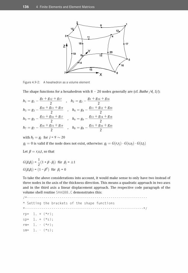
136  4 Finite Elements and Element Matrices

Figure 4.9-2: A hexahedron as a volume element

The shape functions for a hexahedron with 8 ~ 20 nodes generally are (cf. Bathe /4, 5/):

h1 = g1 −g9 + g12 + g17

2, h2 = g2 −

g9 + g10 + g18

2

h3 = g3 −g10 + g11 + g19

2, h4 = g4 −

g11 + g12 + g20

2

h5 = g5 −g13 + g16 + g17

2, h6 = g6 −

g13 + g14 + g18

2

h7 = g7 −g14 + g15 + g19

2, h8 = g8 −

g15 + g16 + g20

2

with hj = gj for j = 9 ∼ 20

gj = 0 is valid if the node does not exist, otherwise: gj = G(r,rj) · G(s,sj) · G(t,tj)

Let β = r,s,t , so that

G(β,βj) =12(1 + β · βj) für βj = ±1

G(β,βj) = (1 − β2) für βj = 0

To take the above considerations into account, it would make sense to only have two instead of three nodes in the axis of the thickness direction. This means a quadratic approach in two axes and in the third axis a linear displacement approach. The respective code paragraph of the volume shell routine SHAQ88.C demonstrates this:/*-----------------------------------------------------------

* Setting the brackets of the shape functions

*----------------------------------------------------------*/

rp= 1. + (*r);

sp= 1. + (*s);

rm= 1. - (*r);

sm= 1. - (*s);

9■■ 9.1 General Information

Two free programs form the basis of this book: Z88V14 Open Source and Z88Aurora V2. While the Open Source version works especially basis-oriented and “originally”, at which you, with the help of the provided source code, can understand all theoretical basics of the previous chap-ters, our new development Z88Aurora provides a very comfortable user interface, which com-pared to Z88V14 Open Source perceptibly facilitates the FE calculation in everyday studies but also in industrial practice. While you work directly with input files and output files in the Open Source version, these files (which are identical for Open Source version and Z88Aurora) are automatically created by Z88Aurora, and you can, e.g., very comfortably apply boundary condi-tions.All static linear examples of this book of course can be calculated with both Z88 versions, and it is up to you to decide which version you use to work through the examples. If you want to work very comfortably from the beginning on and if you are less interested in the program backgrounds, you should choose Z88Aurora V2, with which the use is very similar to commer-cial programs. If you want to know everything in detail, you are not annoyed by a relatively simplistic user interface and you want to study or even change or extend the program code, then give Open Source Z88V14 a try.As you know, both program versions come from our department: Z88V14 Open Source and Z88Aurora V2 are at the moment respectively the newest versions, and in the internet you will find revised and actual releases under www.z88.de.

Z88: The Basics

290  9 Z88: The Basics

9.1.1 Summary of the Z88 Element Library

Two-dimensional Problems: Plane Stress Elements, Plates, Beams, TrussesPlane stress element no. 3 � Shape functions quadratic, but straight boundaries � Quality of displacements: very good � Quality of stresses in the centre of gravity: good � Computing effort: average � Size of element stiffness matrix: 12 × 12

2

X

5

3

1

4

6

Y

Figure 9.1-1: Plane stress element no. 3

Plane stress element no. 7 � Quadratic isoparametric Serendipity element � Quality of displacements: very good � Quality of stresses in the Gauss points: very good � Quality of the stresses in the corner nodes: good � Computing effort: high � Size of element stiffness matrix: 16 × 16

5

4

X

Y

7

8

12

3

6

Figure 9.1-2: Plane stress element no. 7

In this chapter, 32 examples (with other sub examples) are covered, of which the examples 1 to 24 can be carried out with the Open Source version of Z88 as well as with the Z88Aurora Free-ware. The examples 25 to 32 are especially designed for the use of Z88Aurora. For all examples, the respective input files are in the correspondent directories “Z88 V14” and “Z88Aurora” on the DVD. Only the calculation must be carried out. You can import all files of Z88V14 in Aurora; as it is explained later. The examples 4, 6, 7, 13, 17 and 18 can easily be analytically recalcu-lated.The first examples are described very detailed and step by step, so that you can get familiar with the procedure very quickly. Then the later examples require the knowledge of how to use Z88, and they concentrate more on the background of the respective job. The first examples are easy, then they gradually become more complicated, hence, you should work through the examples in sequence.If examples do not start, a memory problem can be on hand. Do other programs require memo-ry, particularly these fat and greedy memory eaters like office packages? All examples were tested on the different computer systems and operating systems, and the smaller examples run even on older computers. Current PCs compute very big Z88 structures without any problems as shown in example 21. The biggest computed structure up to now had 12 million degrees of freedom and ran on a 64 bit PC with 64 bit Windows or with 64 bit LINUX. Adjust Z88.DYN if necessary. Mind the .LOG files: If the memory does not suffice, it is noted in this file.After you have tried the prepared examples, you should design your own examples in your CAD system. Export your models/drawings with a CAD system compatible to AutoCAD as DXF files and convert them with Z88X to Z88 files for Z88 V14 OS or to a STL or STEP file for Z88Aurora. If the Z88-DXF converter Z88X does not convert your DXF files properly, then particularly re-peat the steps 3 and 5 of the chapter 10.7.2. If nothing works, try another CAD program.Do you have a 3D CAD system with an integrated automesher? Then you can export FE meshes in ANSYS-PREP7, COSMOS or NASTRAN format and convert them to Z88 input files with Z88G or Z88ASY in Z88 V14 OS or with the import function in Z88Aurora.Tips for Z88 V14:The import and export files are shown partially shortened so to not fill sides needlessly. Only the essentials should be shown. You can start all examples any time yourself.

Examples13

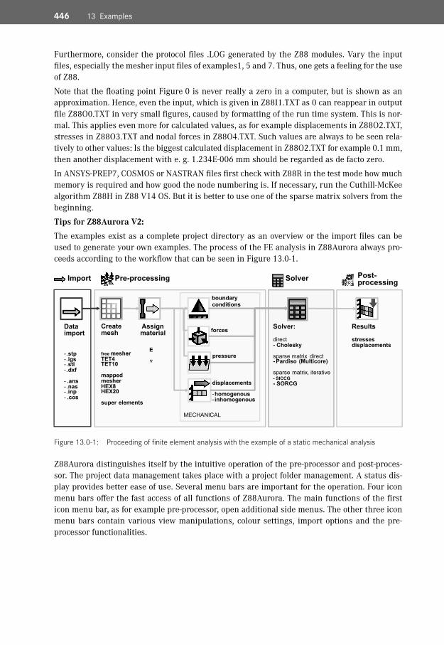
Furthermore, consider the protocol files .LOG generated by the Z88 modules. Vary the input files, especially the mesher input files of examples1, 5 and 7. Thus, one gets a feeling for the use of Z88.Note that the floating point Figure 0 is never really a zero in a computer, but is shown as an approximation. Hence, even the input, which is given in Z88I1.TXT as 0 can reappear in output file Z88O0.TXT in very small figures, caused by formatting of the run time system. This is nor-mal. This applies even more for calculated values, as for example displacements in Z88O2.TXT, stresses in Z88O3.TXT and nodal forces in Z88O4.TXT. Such values are always to be seen rela-tively to other values: Is the biggest calculated displacement in Z88O2.TXT for example 0.1 mm, then another displacement with e. g. 1.234E-006 mm should be regarded as de facto zero.In ANSYS-PREP7, COSMOS or NASTRAN files first check with Z88R in the test mode how much memory is required and how good the node numbering is. If necessary, run the Cuthill-McKee algorithm Z88H in Z88 V14 OS. But it is better to use one of the sparse matrix solvers from the beginning.Tips for Z88Aurora V2:The examples exist as a complete project directory as an overview or the import files can be used to generate your own examples. The process of the FE analysis in Z88Aurora always pro-ceeds according to the workflow that can be seen in Figure 13.0-1.

MECHANICAL

boundary conditions

forces

pressure

displacements

-homogenous - inhomogenous

Assign material

E

Create mesh

free mesher: TET4 TET10 mapped mesher: HEX8 HEX20 super elements

Solver:

direct - Cholesky

sparse matrix, direct - Pardiso (Multicore)

sparse matrix, iterative - SICCG - SORCG

Results:

stresses displacements

Data import

- .stp - .igs - .stl - .dxf - .ans - .nas - .inp - .cos

Pre-processing Solver Post- processing Import

Figure 13.0-1: Proceeding of finite element analysis with the example of a static mechanical analysis

Z88Aurora distinguishes itself by the intuitive operation of the pre-processor and post-proces-sor. The project data management takes place with a project folder management. A status dis-play provides better ease of use. Several menu bars are important for the operation. Four icon menu bars offer the fast access of all functions of Z88Aurora. The main functions of the first icon menu bar, as for example pre-processor, open additional side menus. The other three icon menu bars contain various view manipulations, colour settings, import options and the pre-processor functionalities.

446  13 Examples

13.25 Submarine made of Shells No. 22  677

■■ 13.25  Submarine made of Shells No. 22

A submarine („U-boat“) of class 212A of the German Navy, which was constructed as a shell structure in Pro/ENGINEER is imported into Z88Aurora with the help of NASTRAN and thick-ened to a volume shell. We calculate the deformation and the stresses of the submarine body at a diving depth of 50 meters. The submarine is in a state of poise in the water. This is why we fix it in Z88Aurora with a virtual fixed point, “floating” in the space.

Figure 13.25-1: Geometry of the submarine designed in Pro/ENGINEER

Create a new Project Directory

Create a new project directory .

Import NASTRANThe example file u-boat.nas from z88_examples_z88aurora/b25/Nastran-File is imported as a NASTRAN file with the import object menu. Select the import option “shell”.

Modelling the FE Structure out of SuperelementsIn the next step, we want to mesh the conventional shell structure of the submarine to volume shells. Switch to the Pre-processor menu → Super elements. The volume shell structure should be 20 mm thick:1. Set thickness: Value “20”.2. Administration: “Add” the new meshing rule.3. Generate FE structure: “Create mesh”.

678  13 Examples

Conventional shell hell

Volume shell

Thickness 20 mm

Clipping menu

Clipping menu

Clipping

Figure 13.25-2: Modelling the volume shells

ClippingWith the help of the clipping function we can control that the conventional shell structure has been thickened to volume shells.

Suppress part sections in the current view

Suppress in X-, Y-, Z- direction

SXX

Flip direction of cutting

ng

Clipping

Figure 13.25-3: Clipping menu

13.25 Submarine made of Shells No. 22  679

Assigning the MaterialUse structural steel S235JR from the Z88Aurora material database.

Surface picking – Node pickingSwitch to the “picking context menu” and “node picking” and set to node sets, called “X_direction” and “Z_direction”, for the virtual fixed point. Besides, the surface set “shell sur-face” has to be created. This surface set represents the whole exterior surface of the submarine and contains the boundary condition of pressure. Select a surface facet in the context menu “surface picking”, put the slider for selecting the “angle” to value “50” and pick the whole exte-rior surface by using the button “surface”.

Z_Direction

X_Direction

Nodes 92424, 92431 and 92433

Nodes 92476 and 93022

Figure 13.25 4: Node sets for virtual fixed point

Boundary ConditionsButton Pre-processor → assigning boundary conditions → In the context menu, we assign bound-ary conditions to the node sets and the surface set. A hydraulic pressure of 0.5 N/mm2 is set to the whole shell surface. The node sets are fixed in a way that guarantees statically defined sup-port but lets the submarine “freely” flow in the water.

680  13 Examples

1. Support: Set “Z_direction”, direction X, Y, “displacement”, value “0”, name “XY_locating_support”.2. Support: Set “X_direction”, direction Y, Z, “displacement”, value “0”, name “YZ_locating_support”.3. Pressure: Set “shell surface”, pressure, value “0.5”, name “hydraulic_pressure”.

„XY_fixed“: displacement in X-, Y-direction = 0

„YZ_fixed“: displacement in Y-, Z-direction = 0 t i Y ZY di tt i YY

„Waterpressure“: pressure, 0.5 “

�

Figure 13.25-5: Boundary conditions

Launching the CalculationStart the calculation with the “PARDISO solver”.

OutputsThe PARDISO solver delivers following displacements and stresses in the corner nodes:

�

Figure 13.25-6: Display of the results: displacements

13.25 Submarine made of Shells No. 22  681

Figure 13.25-7: Display of the results: reduced stresses in the corner nodes according to von Mises

Figure 13.25-8: Display of the results inside the submarine: reduced stresses in the corner nodes according to von Mises