)

Transportation Research Record 1008 63

Finite-Element Analysis Applied to the Response of Buried FRP Pipe Under Various Installation Conditions

KEVAN D. SHARP, LOREN R. ANDERSON, A. P. MOSER, and RONALD R. BISHOP

ABSTRACT

Finite-element analysis applied to flexible pipe systems requires capabilities not included in conventional finite-element analysis computer programs. Because of the flexibility of the fiberglass-reinforced plastic pipe and other pipes of similar flexibility, the finite-element analysis may need to accommodate large deflections. In addition, the sensitivity of the pipe and the soil properties to compaction loading should be considered. In this study the stress history of the soil elements was monitored at each loading increment to determine whether each element was to be analyzed by using primary loading nonlinear elastic parameters or unloading and reloading stress-dependent elastic parameters. The development of the additional features of the finite-element computer program allowed for applications to buried flexible pipe when subjected to various in­stallation conditions, backfill material types, surcharge loadings, and inter­nal pressurization. Results of the finite-element analysis applications were compared with measured pipe responses from similar soil-box installation condi­tions. The features of the finite-element analysis computer program and results for a silty sand backfill material under several installation conditions are described. The results are compared with the measured response of the pipe from soil-box tests.

Finite-element analysis (FEA) has been used for several years to predict the response of buried pipes. Several computer programs have been developed that specifically analyze soil-structure systems (l-3; 4,pp.425-430). The development and use of fi­nTt;-element techniques to analyze the response of buried flexible fiberglass-reinforced plastic (FRP) pipe are described. The response of the pipe when subjected to various installation and static loading conditions as computed by the finite-element method was compared with measured strains and deflections taken from physical tests in a soil box at the Buried Structures Laboratory at Utah State Univer­sity. The finite-element soil-structure system modeled the actual soil-box installation conditions. The stress-strain soil parameters that were used in the FEA were obtained from triaxial shear tests per­formed on the soils used in the soil box.

SOIL-BOX TESTS

The details of soil-box tests have been given by Knight and Moser (~) and by Medrano et al. <il· Two soil cells were used, one for pipes with up to 28-in. diameter, the other for up to 60-in. diameter. They can simulate up to 100 ft of overburden pres­sure by means of hydraulic pistons. Pipe diameters of 6, 24, and 48 in. were used in these studies. Pipe stiffness (defined by ASTM D-2412) ranged from 10 to 200 psi. The moment of inertia, modulus of elasticity, and pipe diameter are required to per­form the FEA. Pipe elasticity was measured to be fairly linear in pressure ranges used in the FEA. various installation conditions including poor haunches, soft tops, and varying degrees of homo­geneous compaction were tested. Pipe response was measured by means of strain gauges and a pipe pro­f ilometer !il· Tests were performed on four differ­ent soil types, including washed sand, silty sand, clean gravel, and lean clay. Strain plots and load

deflection plots for each installation condition and soil type have been presented by Knight and Moser (5) and by Medrano et al. (6). Long-term creep ef­f;cts were found to be negligible in the soil-box studies. The FEA and physical test results given in this paper are for the silty sand only. Results for the other cases have been given by Sharp et al. (1_).

FINITE-ELEMENT MODELING OF BURIED PIPES

Analyzing soil-structure systems, such as flexible buried pipes, by the FEA requires sever al special features of the computer model. The models must in­corporate nonlinear stress-strain soil propertiesi structural elements that transfer shear, thrust, and momenti and in some cases interface elements to al­low movement between the soil and structure (1,8,9). Soil models that have been developed generally-take into account the stress dependency of the elastic moduli of the soil. These soil models are used with an incremental linear FEA (iterative procedure) that of necessity must model the construction sequence. Two-dimensional plane strain soil elements of var­ious types have been developed that are used in con­j unction with the structural beam elements. Inter­face elements have also been developed that account for differential displacement at the soil-structure interface (_!,~,~). Katona <!.Q_l and Leonarda et al. (11) have shown that interface slip is important for FEA of buried pipes when deflections are large. Dun­can (8) and Nyby (9), on the other hand, suggest that the use of int;rface elements is of only minor importance for most cases. In this study interface elements were not used in order to simplify the com­parative analysis for evaluating the importance of stress history, compaction simulation, and geometric nonlinearities. Even though interface elements were not used, the general conclusions of the study are valid, because FEA results compared favorably with experimental data.

64

Buried-pipe analysis using finite-element tech­niques generally requires modeling the construction sequence of the installation for either an embank­ment or a trench. Foundation, bedding, and fill material are generally included as separate soil types within the finite-element mesh.

In order to compare FEA simulations with soil­cell tests, it was desired to model the following conditions:

1. Various installation conditions including poor haunches, low soil density at the pipe crown, effect of trench width, homogeneous compaction of the backfill with low and high relative compaction, sheeting installation, and nonsymmetric beddingi

2. Backfill material type including clean sand, clean gravel, silty sand, and lean clay;

3. Initial ovalization of the flexible pipe caused by compaction during constructioni

4. Rerounding induced by internal pressurization of the deformed pipei and

5. Collapsing soil structure under bedding due to groundwater fluctuations in moisture-sensitive soil.

The FEA computer program that was used in this study was originally developed by Wilson (Ql and Ozawa and Duncan (2), and most recently modified by Duncan et al. (13), whose version of the computer program, SSTIPN,~includes soil and structure ele­ments as well as interface elements. The soil stress-strain characteristics are modeled by hyper­bolic parameters as presented by Duncan et al. (_!2). The hyperbolic parameters model stress- and strain­dependent elastic and bulk moduli. Shear moduli and Poisson's ratios are computed by using relationships from the theory of elasticity. The computer program SSTIPN was modified as a part of this study to spe­cifically accommodate analysis of flexible pipe de­formation. These enhancements affected the soil model, iteration scheme, element stiffness matrices, and output.

SOIL MODEL

The Duncan soil model uses hyperbolic relationships to model the nonlinear behavior of soil elasticity. The modulus of elasticity is computed as a function of the hyperbolic equations and percentage of mobil­ized strength. This accommodates the behavior of soil elasticity in which there is a high modulus at initial strain that decreases as the percentage of mobilized strength increases. One of the shortcom­ings of the soil model is that nonlinear equations are used to model inelastic behavior of soil. Figure 1 shows a stress-strain curve for a soil sample in a triaxial shear test. The loading sequence for the sample was to increase the vertical stress until the sample had undergone initial strain, then to unload the sample, and finally to reload the sample until failure. In Figure 1 it can be seen that the sample has a nonlinear stress-strain response on primary loading. The unloading and reloading characteristics below the previous maximum past pressure, however, .do not follow the initial primary curvei they show an inelastic response. After reloading beyond the maximum past pressure, the stress-strain curve again follows the initial nonlinear primary loading curve.

Duncan et al. <ill discuss the behavior of soil on unloading and reloading in comparison with that on primary loading. The soil stiffness is reported to be 1.3 to 3.0 times greater when in the overcon­solidated range. Volumetric strain is reported to be unaffected by stress history. Triaxial testing for unloading and reloading in this study has shown that

Transportation Research Record 1008

60

iii !!:. IJ) IJ)

40 w a: ~ IJ)

a: 0 20 ~ c(

> w 0

J 10

% STRAIN

FIGURE 1 Devialor stress versus strain for triaxial soil specimen showing primary loading, unloading, and reloading.

the magnitudes of the hyperbolic constant and expo­nent depend on whether the soil is in primary load­ing or unloading and reloading <2,14). Testing for behavior of volumetric strain was also performed, but no specific conclusions could be reached for bulk modulus effects.

It was necessary to model stress history for each soil element in this study because of the need to model initial deformation of the pipe due to compac­tion. Some of the soil elements should respond in the rebound range because of compaction until the surcharge pressures exceed compactive loading pres­sures. Also, the study involving rerounding of the pipe required that the soil elements respond appro­priately as the pipe rerounds when internal pressure is added to the loading sequence. Because the soil is much stiffer in the rebound range, the pipe de­formation is dependent on the stress history of the soil. Not all the soil elements in the finite-ele­ment mesh will respond to the rebound range at any given time as the pipe rerounds or as the compaction loads are modeled. Thus, it is necessary to monitor the stress history of each soil element during the analysis and use appropriate stiffness parameters depending on the current stresses of each element. A technique for accommodating these features was developed and incorporated in the computer model.

The stress history of the soil elements is moni­tored by evaluating the position of the center of Mohr's circle for each element (the average stress). The average stress at any load increment is compared with the maximum average stress from previous incre­ments. If the average current stress is less than the maximum previous stress, the soil elastic modu­lus is computed by using the unloading and reloading parameters. Likewise, the soil elements are moni­tored in the rebound range and will convert to the primary loading curve when the average current stresses exceed the maximum past average stress. This method thus allows simulation of soil element response for any soil element on either rebound or primary loading, depending on the loading conditions and soil response. Two additional soil parameters are required as inputs for the Duncan soil model that account for the behavior of the soil in the un­loading and reloading range.

MODIFIED ITERATION PROCEDURE

The FEA solution for nonlinear response is generally modeled by using an iterative scheme. Because the stiffness matrix requires the element stresses in order to compute the stress-dependent elastic param­eters, some initial estimate of the stresses is re­quired. The finite-element scheme computes the re­sulting nodal,deflections and corresponding stresses and strains. An iterative procedure follows that uses the newly computed elastic parameters.

Sharp et al.

The iterative scheme in SSTIPN uses the elastic parameters from the previous load increment to com­pute new stresses on the first iteration of the cur­rent load increment. The second iteration uses an average of the new stresses and the previous stresses for evaluation of the elastic moduli. The resulting stresses and strains from the second iteration are the final stresses and strains for the current increment. No additional iterations follow, and convergence is not evaluated. The justification for such an iteration scheme is that the average stresses used in the second iteration are very close to the final stresses that will result if iteration to convergence is allowed. This assumption is valid in view of the many other approximations that are inherent in the analysis, including idealized back­fill conditions, approximations in the finite-ele­ment scheme, and inexact soil modeling.

The incorporation of the modeling of the soil by using the stress history to determine the soil con­dition requires a slightly different iteration scheme. The appropriate soil model to be used for any element cannot be determined until after the first iteration on which the stresses are compared with the previous maximum past average stress. Be­cause the first iteration uses the elasticity param­eters from the previous load increment, the second iteration uses the appropriate elastic moduli either from unloading and reloading or primary loading parameters based on the results from the first iteration. The original sequence would then have used average stresses resulting from the first iteration and previous load increment to evaluate the elastic moduli for the second iteration. How­ever, if the soil model has changed from either un­loading-reloading to primary loading or vice versa, the results from the second iteration would not be close enough to convergence. A new iteration se­quence was incorporated that uses a second iteration similar to the old first iteration, with the appro­priate soil elastic parameters. In addition, a third iteration using average stresses follows similar to the second iteration on the original scheme. The user also has the option to specify additional iterations for each increment, but a convergent scheme such as Newton-Raphson for systems of equa­tions is not incorporated. Studies have shown that four iterations appear to be sufficient when the modified soil model is used.

GEOMETRIC NONLINEAR ANALYSIS

The basis for the development of the finite-element scheme for soil-structure interaction uses small-de­flection theory. However, for certain applications, it is desirable to incorporate large-deflection theory in the finite-element scheme. The isopara­metr ic elements that are used in this study require the stiffness matrix for soil elements to be reeval­uated at each increment. The portions of the element stiffness matrix based on element geometry were modified because of deforming coordinates by merely changing the coordinates of the nodes based on the deflections from the previous increment. Modifica­tion to the structural stiffness matrix was also in­cluded by reevaluating the structural stiffness matrix at each increment based on new element lengths due to deformations from previous itera­tions. This includes large-deflection theory into the finite-element scheme but does not incorporate the higher-order terms in the element stress-strain relationships.

Incorporation of the deforming nodes into the element stiffness matrix allowed several aspects of flexible pipe deformation to be analyzed. For ex-

65

ample, it was possible to analyze rerounding due to internal pressure. Pipe rerounding cannot be simu­lated if the structural stiffness matrix does not recognize the pipe deformation before internal pres­surization. Large-deflection theory also allows for the analysis of the pipe response due to initial ovalization from compaction loads. Very flexible pipes frequently are deformed at compaction. This deformation is generally upward at the crown because of compaction at the springline and shoulders. By incorporating the compaction load sequence in addi­tion to geometric nonlinear analysis, the pipe re­sponse is automatically computed based on its de­formed shape after the construction sequence is complete and before surcharge loads are added.

POSTPROCESSING CAPABILITIES

In order to expedite the analysis of the results from each condition, postprocessing capabilities were developed. The postprocessing routines were in­cluded by organizing and modifying some of the out­put results in such a way as to accommodate plotting routines specifically designed for pipe response analysis. Load-deflection curves, pipe strain, mo­ment and shear plots around the pipe circumference, pipe deformation, and element mesh deformation plot­ting capabilities were developed.

APPLICATIONS TO ANALYSIS OF FIBERGLASS PIPE PERFORMANCE

The research program involving buried FRP pipe per­formance consisted of several tasks. The development of the FEA modifications was only one of the major tasks that were to be accomplished. With its devel­opment, the applications of FEA to numerous soil types, backfill conditions, and loading conditions were performed. The approach that was taken in the study was to simulate the backfill and loading con­ditions that had been used in the soil-box tests in order to compare the predicted response of the pipe from FEA results with the measured response. This required that the four soils that were used in the soil box be tested for engineering properties, in­cluding triaxial testing at several densities for evaluation of the hyperbolic parameters for the Dun­can soil model. Results from the tests are described by Sharp et al. (14). In the following discussion, only the results of the applications of the finite­element program to the installation conditions for silty sand will be presented. The results of the re­maining applications are included in the report by Sharp et al. (2).

Determination of Duncan Soil Parameters

The silty sand that was used in the soil-box tests is characterized as a nonplastic material with about 40 percent passing the 0.075-mm sieve and about 10 percent clay-size particles. Maximum dry density of the silty sand is 124.7 lb/ft' and the optimum water content is 9. 5 percent based on AASHTO T-99 compaction.

Triaxial shear testing of the silty sand was per­formed by using samples compacted at water contents similar to those used in the soil-box tests. Elastic modulus and bulk modulus parameters are required in the FEA for each density. Testing of the clean gran­ular materials (washed sand and gravel) was per­formed by using saturated samples, and the volume change was monitored by measuring the volume of water extruded or imbibed in the samples during

66

drained shear. Because the stress-strain and strength properties of the silty sand and clay are dependent on drainage, density, compaction water content, and water content at shear, it was neces­sary for the soil parameters to represent field con­ditions as much as possible. Therefore, the silty sand and the clay were tested by using unsaturated undrained conditions. The triaxial equipment was not equipped to measure volumetric strain of undrained samples, and thus bulk modulus parameters were not measured for the fine-grained soils (silty sand and clay).

Triaxial testing was performed on the silty sand at three different densities (95, 80, and 77 percent relative compaction based on Standard Proctor) • Stress-strain curves were obtained for three confin­ing pressures within the range of confining pres­sures used in the soil-box tests for each density. The triaxial testing procedure involved preparing the sample with compaction techniques similar to those in the field and applying the deviator by ini­tial loading, unloading, and reloading to failure. This resulted in data that were interpreted with procedures outlined by Duncan et al. (13) for deter­mination of shear strength and the hyperbolic param­eters for the elastic moduli. The unloading and re­loading data were also evaluated to obtain the rebound parameters for each density.

Because data were not obtained for the hyperbolic bulk modulus parameters, an FEA sensitivity study was performed by using soil-box test results to calibrate the silty-sand data. Soil-box tests were performed on the silty sand by using 90 and 80 per­cent relative compaction. The elastic moduli for the 90 percent relative compaction were obtained by interpolating the measured values from the 95, 80, and 77 percent relative compaction data. Sensitivity studies were performed by using a 90 percent homo­geneous relative compaction and an BO percent homo­geneous relative compaction in the finite-element mesh to determine the bulk modulus parameters. These sensitivity studies show that the shape of the load­deflection curve can be adjusted by modifying the bulk modulus exponent. Pipe strain plots can also be adjusted because of complex interrelationships be­tween hyperbolic elastic and bulk modulus parameters in conjunction with the shear strength of the soil. Table l shows the final values for the soil param­eters that were used for the silty sand at 90 per­cent and BO percent relative compaction. A more com­plete description of the sensitivity studies is contained in the report by Sharp et al. <2>·

Finite-Eiement Modeling

The modeling of the fiberglass pipe response by using silty sand as backfill material consisted of several installation conditions and 10- and 100-psi pipe stiffnesses (ASTM D-2412) • Installation condi­tions included homogeneous compaction at 90 and BO percent relative compaction, poor haunches, and soft crown. In general the poor-haunche and soft-crown conditions were obtained by not compacting the soil

Transportation Research Record lOOB

in these areas. Figure 2 shows the finite-element mesh and soil materials or types that were used in this study. The poor-haunch condition used 90 per­cent relative compaction for all soil types except that in the haunches (soil type 6) • The soft-crown condition used 90 percent relative compaction for all soil types except that in the area from the shoulders to the crown of the pipe, shown in Figure 2 as soil type 7. These installation conditions were used because of the way in which materials were placed around the pipe during installation. When the pipe has low stiffness, it is difficult to compact the fill material over the crown until sufficient cover has been placed. Also, extra effort is re­quired to compact the soil in the haunches, so it was desired to model installation conditions in which there was l oose material in the haunches. The other soil types that are shown were included to in­vestigate effects due to split installation, diffe­rent foundation materials, and other types of in­stallations.

The finite-element modeling scheme consisted of two phases. The first modeled construction incre­ments without compaction simulation. Four installa­tion conditions were modeled for pipes with stiff­nesses of 10 and 100 psi. The second incorporated a compaction simulation on each construction increment before the next construction increment was added. Three installation conditions were modeled by using the compaction simulation. Table 2 shows the instal­lation conditions that were used for the silty sand and indicates those that included compaction simula­tion.

Soil elements in the foundation and up to the springline (soil materials 1 through 3) were treated as preexisting elements having stresses and strains predefined at the time of program execution. In the construction sequence used in the first phase, placement of the remainder of soil 3 and all of soils 4 and 7 was simulated as the first construc­tion increment. The second construction increment completed the mesh by placing soil material s.

The second phase of the modeling incorporated compaction simulation after each construction se­quence. The compaction simulation involved addition and removal of compaction loads at the end of the first and second construction increments. The first compaction load was added to the first layer of soil material 4. The second compaction loading was placed on the completed mesh over soil material 5. It was found that the first loading sequence was critical in inducing initial ovalization of the pipe. It was not possible to load directly over the pipe (soil material 7) without causing structural failure and large unrealistic deformation of the pipe and soil because of an unstable condition. This result ap­pears to be in accordance with the actual installa­tion conditions, in which it was found that effec­tive soil compaction could not be performed over the pipe until sufficient cover had been placed. Also, it was not possible to add compaction loads on the soil before placement of the first increment. When loads were added adjacent to the springline on soil material 3, pressures caused excessive deformation of the pipe.

TABLE I Soil Parameters for Silty Sand

RC density "' /':; c K n Rt Kb m Ko Kur nur

Stand. lb/in' deg deg psi

90% 0.065 30 0. 8.3 480 .44 .75 80 .38 .48 720 .44

80% 0.058 30 o. 3.5 350 .28 .89 15 .40 .37 525 .28

Note: See report by Duncan et al. (13) for definitfon of parameters ,

Sharp et al. 67

TABLE 2 Installation Conditions for Silty Sand

Condition

·1. 90% homogeneous

2. 90% backfill with soil top@ 80% RC

3. 90% backfill with soft lop@ 77% RC

4. 90% backfill wilh haunches@ 80% RC

5. 90% backfill wilh haunches@ 79% RC

6. 90% backfill wilh haunches@ 77% RC

Pipe Stiffness

(psi)

10, 100

10, 100

10

10, 100

10

10

Compaction Simulation

yes

yes

no

yes

no

no

7. 90% backfill with top and haunches@ 85% RC 10 no

8. 80% homogeneous

For compaction simulation, a uniform static load of 10 psi was used corresponding to the type of com­paction equipment used in the soil-box test. A more rigorous compaction sequence would have been to load each soil element individually with a larger pres­sure, which would result in a better simulation of the compaction process. The load of 10 psi was deemed an equivalent surface pressure over a large area. The compaction load was added in two incre­ments of 5 psi each. After the compaction load had been placed, a sequence of unloading was followed. A series of unloading steps in small pressure incre­ments was followed until the elements in the top row of the mesh approached a tension condition with negative confining pressure. Small increments were used in the loading and unloading sequence in order to assure that the soil elements were being evalu­ated correctly for either the primary loading or re­bound parameters. Magnitudes that were too large for compaction loading might have caused poor conver­gence and incorrect evaluation of the appropriate soil response model. It was not possible with the silty sand to remove the same load magnitude that was "placed without causing tension failures in all elements in the mesh. This was not the case with the clay analysis, however, because it was numerically possible to remove the same quantity of compaction load that was placed. Although it may seem invalid to model compaction loading without removing the same load that was placed, it must be pointed out that the solution is an incremental loading proced­ure. The total load vector is not evaluated at each iteration. Only the total stresses and strains in each element are evaluated. Thus although success at unloading the elements with the same compaction load magnitude was not achieved, it was possible to in­duce stress history in the soil due to compaction loads, which resulted in allowable soil stresses, strains, and deformations.

The inability to unload the soil element com­pletely without complete tension failure might be attributed to numerical approximations with the fi­nite-element technique. Problems arise in the soil model in evaluating Poisson's ratio when the soil is in the unloading and reloading range. Poisson's ratio is computed by using the theory of elasticity relationships between bulk modulus and elastic modu­lus, When the elastic modulus increases as in un­loading and reloading, Poisson's ratio is computed at its minimum of 0.0 if the bulk modulus does not increase proportionately. Behavior of the bulk modu­lus is difficult to determine on unloading and re­loading relative to primary loading. Sharp et al. (14) tested bulk modulus behavior in triaxial shear of saturated drained granular material for primary loading as well as rebound loading. It was not pos­sible to conclude how volumetric deformation behaves

10, 100 no

as a function of stress history for the coarse­grained material. In addition, the granular material exhibited dilation at a small strain (a response that cannot be acconunodated with the theory of elas­ticity).

RESULTS OF APPLICATIONS

The results of the applications of the FEA were com­pared with the measured response from the soil-box tests. The comparisons that are shown in this paper are for the pipe with 10 psi stiffness only. Soil­box compaction conditions that were used for com­parisons were 90 percent relative compaction with homogeneous conditions, 90 percent relative compac­tion with poor haunches, and 80 percent relative compaction with homogeneous conditions. In the soil­box testing, every attempt was made to achieve homo­genous conditions. However, as noted, the flexible nature of the pipe does not always allow for thorough compaction in the haunches and around the shoulders and crown of the pipe. Therefore, for the homogeneous conditions that were attempted in the soil box there was actually some variability in density. When the pipe was installed with poor haunches in the soil box, no attempt was made to compact the soil. Finite-element modeling of homo­geneous and poor-haunch conditions is better defined because numerically all soil elements in a homo­geneous condition have identical stress-strain prop­erties.

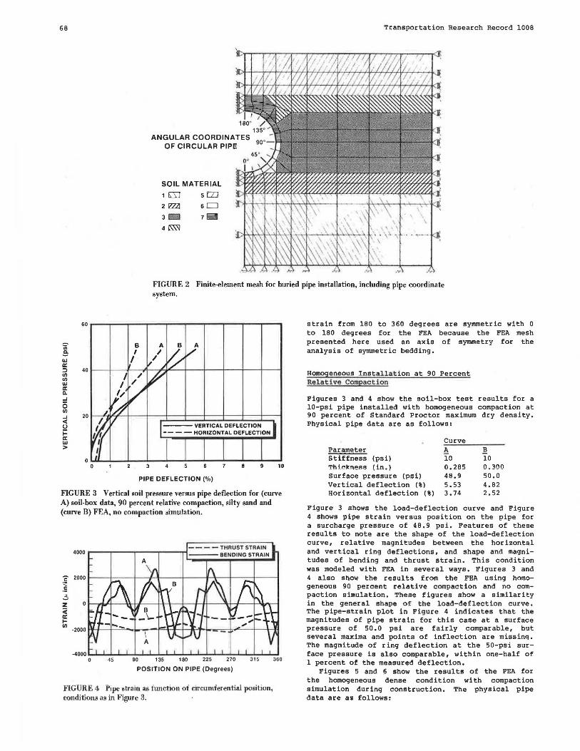
Comparisons of the FEA results with those of the soil-box tests were made by using pipe-strain and load-deflection results. The pipe-strain plots indi­cate the bending strain in the outside fibers (ten­sion is positive) and thrust strain around the cir­cumference of the pipe for a given surcharge pressure. The load-deflection plots indicate the vertical and horizontal ring deflections (the ratios of change in vertical and horizontal diameters to initial diameter) versus surcharge pressure. In the soil-box tests, the load-deflection plots were referenced to the deformed state of the pipe after compaction. In the FEA plots, the reference of ring deflection is based on the initial undeformed condi­tion. Thus in the comparison of figures that fol­lows, the zero point of deflection should be con­sidered when direct comparisons of load deflections between the FEA and the soil-box tests are per­formed. Pipe-strain plots for both soil-box and FEA results were referenced from the same unstrained condition. The pipe-strain plots show bending and thrust strain versus position on the pipe. Zero degrees on the pipe is at the invert, 90 degrees is at the springline, and 180 degrees is at the crown as shown in Figures 2 and 3. The values for pipe

68

SOIL MATERIAL

1 rn s l'.ZJ 2 l?Z2l 6 CJ 3 lmm 7~

4~

Transportation Research Record 1008

FIGURE 2 Finite-element mesh for buried pipe installation, including pipe coordinate system.

'iii c. w cc ::::> (/) (/) w cc c.

= 0 (/)

_J

ct u ~ cc w >

B A

9 10

PIPE DEFLECTION (%)

FIGURE 3 Vertical soil pressure versus pipe deflection for (curve A) soil-box data, 90 percent relative compaction, silty sand and (curve B) FEA, no compaction simulation.

4000

g 2000

~ ,.:; z < cc I-(/)

-2000

45 90 135 180 225 270 315

POSITION ON PIPE (Degrees)

FIGURE 4 Pipe strain as function of circumferential position, conditions as in Figure 3.

360

strain from 180 to 360 degrees are symmetric with 0 to 180 degrees for the FEA because the FEA mesh presented here used an axis of symmetry for the analysis of symmetric bedding,

Homogeneous Installation at 90 Percent Relative Compact i on

Figures 3 and 4 show the soil-box test results for a 10-psi pipe installed with homogeneous compaction at 90 percent of Standard Proctor maximum dry density. Physical pipe data are as follows:

Curve Parameter ~ !! Stiffness (psi) 10 10 Thickness (in . ) 0.285 0 , 300 Surface pressure (psi) 48.9 50,0 Vertical deflection (%) 5.53 4.82 Horizontal deflection (%) 3.74 2,52

Figure 3 shows the load-deflection curve and Figure 4 shows pipe strain versus position on the pipe for a surcharge pressure of 48.9 psi. Features of these results to note are the shape of the load-deflection curve, relative magnitudes between the horizontal and vertical ring deflections , and shape and magni­tudes of bending and thrust strain. This condition was modeled with FEA in several ways. Figures 3 and 4 also show the results from the FEA using homo­geneous 90 percent relative compaction and no com­paction simulation, These figures show a similarity in the general shape of the load-deflection curve. The pipe-strain plot in Figure 4 indicates that the magnitudes of pipe strain for this case at a surface pressure of 50.0 psi are fairly comparable, but several maxima and points of inflection are missing, The magnitude of ring deflection at the 50-psi sur­face pressure is also comparable, within one-half of 1 percent of the measured deflection.

Figures 5 and 6 show the results of the FEA for the homogeneous dense condition with compaction simulation during construction. The physical pipe data are as follows:

Sharp et al.

Parameter Stiffness (psi) Thickness (in.) Surface pressure (psi) Vertical deflection (%) Horizontal deflection (%)

Curve A 10 0.285 48.9 5.53 3.74

B 10 0.300 so.a 5.42 3.14

The load-deflection plot in Figure 5 has lost some of the initial steepness, but the difference between vertical and horizontal deflection is maintained. Relative to Figure 3, the magnitudes of deflection are similar. Figure 6 shows the pipe-strain plot from the compaction simulation at a surface pressure of 50. 0 psi. Comparison of Figure 6 with the mea­sured values from the soil-box results in Figure 4 shows that compaction simulation did improve the correlation. In fact, the general shape, maxima, and magnitudes all compare very well. This result is the best comparison that was obtained between any soil­box test and FEA result for all soil types and in­stallation conditions.

2 3 6 10

PIPE DEFLECTION (%)

FIGURE 5 Vertical soil pressure versus pipe deflection for (curve A) soil-box data, 90 percent relative compaction, silty sand and (curve B) FEA with compaction simulation.

:5 ~ ..:: z ~ a:

- - - - THRUST STRAIN 4000..-~-,~~.,.~~,-~~ri.:;;;;;;-;_:B~EN;D~l~N~G~S~T~R~A:IN:.11

~ -2000~./-~~:...0..~,_..or"-tO!:\:;v.-l:--1Ff"'+....-;;;;-;;±-.,,._~-+~-\:l·

-4000L.L..L..L..L....L...J...J...J-l.-"-l.~,_i.~~~ ..... ~~---:":::-.I.---~ 0 4' 90 180 380

POSITION ON PIPE (Degrees)

FIGURE 6 Pipe strain as function of circumferential position, conditions as in Figure 5.

Additional comparisons that were made with this condition included soft elements in the shoulders of the pipe. Because techniques did not allow compac­tion above the pipe, a theoretically homogeneous in­stallation would still have soil of a lesser density

69

at the crown. FEA results for this condition in­cluded various degrees of compaction in the shoulders, with and without compaction simulation. These results are not shown in this paper; however, similar load-deflection and pipe-strain plots were obtained. One noticeable result with the soft-crown analyses was that generally the pipe strain at the 135-degree position of the pipe (see Figure 3) in­creased. This is due to the lowered stiffness of the soil in the shoulders, which allows for more bending deformation in the pipe. Compaction simulation for the soft-crown condition did decrease the bending strains and ring deflections because the soil would respond in the rebound range initially, thus in­hibiting deformation at the low pressure ranges. Be­cause compaction simulation did not include adding loads directly over the pipe at the first construc­tion increment, a soft-crown condition was actually created with the homogeneous case. This is because the soil at the crown was uncompacted and did not respond on the stiffer rebound modulus at the lower pressure ranges as did the surrounding soil elements that had received the compaction loads directly.

Poor-Haunch Installation at 90 Percent Relative Compaction

Figures 7 and 8 show the results for the poor-haunch installation with the silty sand in the soil-box tests. The physical pipe data are as follows:

Curve Parameter A B Stiffness (psi) Io Io Thickness (in.) 0.285 0.300 Surface pressure (psi) 35.5 30.0 Vertical deflection (%) 3.14 2.21 Horizontal deflection (%) 1.30 1.09

Figure 7 shows the load-deflection response and Fig­ure 8 shows the pipe strain around the pipe for a surface pressure of 35.5 psi. Again the initial steepness of the load-deflection curve, the relative magnitudes between the vertical and horizontal de­flections, and the shape and magnitude of the strain plots should be noted. The bending strains were higher at the 30- to 45-degree position of the pipe because of the lack of support in the haunch area. Also, a comparison between the homogeneous installa-

·;;; .e w a: ::> (/) (/) w er: ii.

= 0 (/)

..J C( u ~ a: w >

PIPE DEFLECTION (%)

FIGURE 7 Vertical soil pressure versus pipe deflection for (curve A) soil-box data, 90 percent relative compaction, silty sand, and poor haunch support and (curve B) FEA, no compaction simulation, and poor haunch support.

70

4000

2000

~ .E ~

0

z Ci r:c I-(/)

-4000

POSITION ON PIPE (Degrees)

FIGURE 8 Pipe strain as function of circumferential position, conditions as in Figure 7.

tion and the poor-haunch installation in Figures 6 and B, respectively, shows noticeable differences in the pipe-strain plots from soil-box tests. Figures 7 and B also show the FEA results for the poor-haunch condition without compaction simulation. The load­deflection plot shows similar behavior, yet the de­formations are larger in the FEA results. The pipe­strain plot did, however, show a very similar peak of large strain at the 45-degree position and low strains from the springline to crown, similar to the soil-box results, Figures 9 and 10 show the FEA re­sults for poor haunches with compaction simulation. In these results, the load-deflection plots showed larger deflections and the pipe-strain plots had larger strains in the pipe from the spr ingline to the crown than in Figure B. However, the strain at the invert of the pipe with compaction simulation was more comparable with measured results than with the FEA results that did not include compaction simulation. The physical pipe data for Figures 9 and 10 are as follows:

Curve Parameter A Stiffness (psi) 10 Thickness (in.) 0.285 Surface pressure (psi) 35,5 Vertical deflection (%) 3.14 Horizontal deflection (%) 1.30

Hompgeneous Installation with 80 Percen t Relative Compaction

B 10 0.300 30.0 5.14 2.92

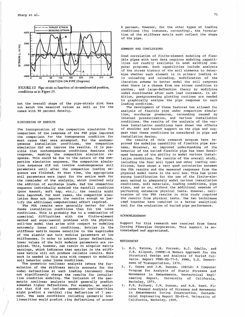
Figures 11 and 12 show the soil-box results for the 80 percent relative compaction homogeneous installa­tion. The physical pipe data are as follows:

Curve Parameter A B Stiffness (psi) 10 10 Thickness (in.) 0.285 0.300 Surface pressure (psi) 14.6 15.0 Vertical deflection (%) B.78 3.85 Horizontal deflection (%) 7.87 2.06

The vertical and horizontal deflections are very similar throughout the test, which indicates ellip­tical deformation as shown in Figure 11. Figures 11 and 12 also show the results from the FEA for the 80 percent relative compaction homogeneous condition. Although the load-deflection curve shows much more

Transportation Research Record 1008

2

PIPE DEFLECTION (%)

FIGURE 9 Vertical soil pressure versus pipe deflection for (curve A) soil-box data, 90 percent relative compaction, silty sand, and poor haunch support and (curve B) FEA with compaction simulation and poor haunch support.

4000

2000

£ E ~

0

z Ci r:c -2000 I-(/)

POSITION ON PIPE (Degrees)

10

FIGURE 10 Pipe strain as function of circumferential position, conditions as in Figure 9.

"iii .e w r:c ::::> (/) (/) w r:c Q,

::! 0 (/)

-' <( u j:: r:c w >

A

10

PIPE DEFLECTION (%)

FIGURE 11 Vertical soil pressure versus pipe deflection for (curve A) soil-box data, 80 percent relative compaction and (curve B) FEA, no compaction simulation.

deformation with the loose material than with the dense material, the actual comparison of soil-box tests with FEA tests shows that the FEA did not com­pare quite as well for the looser condition. The pipe-strain plot shown in Figure 12 also supports the generally poorer comparison. In terms of magni­tude of the maximum strain, there is correlation,

Sharp et al.

~ .!: .; z ct a: 1-U)

FIGURE 12 Pipe strain as function of circumferential position, conditions as in Figure 11.

but the overall shape of the pipe-strain plot does not match the measured values as well as for the cases with 90 percent density.

DISCUSSION OF RESULTS

The incorporation of the compaction simulation for comparison of the response of the FRP pipe improved the comparison for the homogeneous condition for most cases that were attempted. For the nonhomo­geneous installation conditions, the compaction simulation did not improve the results. It is pos­sible that nonhomogeneous conditions dominate the response, masking the compaction simulation re­sponse. This could be due to the nature of the com­paction simulation sequence. The compaction simula­tion sequence did not involve nonhomogeneous soil parameters until after the compaction loading se­quence was finished. At that time, the appropriate soil parameters were input for the entire mesh for the remainder of the analysis, which involved only the addition of surcharge loads. Had the compaction sequence individually modeled the backfill condition (poor haunch, soft top, etc.), the results might have improved. For most cases, the compaction simu­lation does not improve the results enough to jus­tify the additional computational effort required.

The FEA results were generally better for the dense installation conditions than for the loose conditions. This is probably due to a combination of numerical difficulties with the finite-element method and experimental problems with the physical soil-box model that arise with respect to modeling extremely loose soil conditions. Entries in the stiffness matrix become sensitive to the magnitudes of the elastic and bulk modulus parameters at low stiffnesses. In order to achieve larger deflections, lower values of the bulk modulus parameters are re­quired. This, however, can result in singular matrix warnings, which indicates that entries in the stiff­ness matrix will not produce re-liable results. More work is needed in this area with respect to modeling soil behavior under loose conditions.

The geometric nonlinear analysis (where the for­mulation of the stiffness matrix accounts for the nodal deflections at each loading increment) does not significantly change the results for installa­tion condition modeling. The inclusion of the geo­metric nonlinear analysis would generally predict somewhat higher deflections. For example, an analy­sis that did not include geometric nonlinearities might predict a vertical ring deflection of 7 per­cent. The same conditions including geometric non­linearities would predict ring deflections of around

71

8 percent. However, for the other types of loading conditions (for instance, rerounding), the formula­tion of the stiffness matrix must reflect the shape of the pipe.

SUMMARY AND CONCLUSIONS

Good correlation of finite-element modeling of flex­ible pipes with test data requires modeling capabil­ities not readily available in most existing com­puter programs. Such capabilities include analysis of the stress history of the soil elements to deter­mine whether each element is in primary loading or in unloading and reloading, modification of the iteration scheme to better model the soil response when there is a change from one stress condition to another, and large-deflection theory by modifying nodal coordinates after each load increment. In ad­dition, postprocessing plotting routines are needed to graphically analyze the pipe response to each loading condition.

The development of these features has allowed for analysis of flexible pipe under compaction simula­tion, surcharge pressures, rerounding caused by internal pressurization, and various installation conditions. The results of the analysis of the var­ious installation conditions have shown the effects of shoulder and haunch support on the pipe and sug­gest that these conditions be considered in pipe and installation design.

The results of this research program have im­proved the modeling capability of flexible pipe sys­tems. Moreover, an improved understanding of the behavior of the buried flexible pipe has been devel­oped because of the ability to model various instal­lation conditions. The results of the overall study, including the four soil types and other loading con­ditions, have shown a very good correlation between the FEA results and the measured responses from the physical model tests in the soil box. This has given strong justification for the use of the f inite-ele­ment method to adequately model various installation conditions, soil materials, loading conditions, pipe sizes, and so on, without the additional expense of performing extensive physical tests. However, cali­bration of the FEA results in this study required the results from physical tests. The two techniques used together have resulted in a better analytical tool for the evaluation of buried pipe performance.

ACKNOWLEDGMENT

Support for this research was received from Owens Corning Fiberglas Corporation. This support is ac­knowledged and appreciated.

REFERENCES

1. M.G. Katona, J.B. Forrest, R,J, Odello, and J .R. Allgood. CANDE--A Modern Approach for the Structural Design and Analysis of Buried Cul­verts. Report FHWA-RD-77-5. FHWA, U.S. Depart­ment of Transportation, 1976.

2. Y. Ozawa and J.M. Duncan. ISBILD: A Computer Program for Analysis of Static Stresses and Movements in Embankments. Geotechnical Engi­neering Report. University of California, Berkeley, 1973.

3. F.H. Kulhawy, J.M. Duncan, and H.B. Seed. Fi­nite Element Analysis of Stresses and Movements in Embankments During Construction. Geotech­nical Engineering Report TE-69-4. University of California, Berkeley, 1969.

72

4. D.W. Nyby and L.R. Anderson. Finite Element Analysis of Soil-Structure Interaction • .!.!! Pro­ceedings of the International Conference on Finite Element Methods (H. Guangqian and Y .K. Cheung, eds.), Science Press, Beijing, China, 1982.

5. G.K. Knight and A.P. Moser. The Structural Re­sponse of Fiberglass Reinforced Plastic Pipe under Earth Loadings. Buried Structures Labora­tory, Utah State University, Logan, 1983.

6. s. Medrano, A.P. Moser, and O.K. Shupe. Per­formance of Fiberglass Reinforced Plastic Pipe to Various Soil Loads and Conditions. Buried Structures Laboratory, Utah State University, Logan, 1984.

7. K.D. Sharp, L.R. Anderson, A.P. Moser, and M.J. Warner. Applications of Finite Element Analysis of FRP Pipe Performance. Buried Structures Laboratory, Utah State University, Logan, 1984.

8. J.M. Duncan. Behavior and Design of Long-Span Metal Culverts. Journal of Geotechnical Engi­neering, ASCE, Vol. 105, No. GT3, March 1979.

9. D.W. Nyby. Finite Element Analysis of Soil­Structure Interaction. Ph.D. dissertation, Utah State University, Logan, 1981.

10. M.G. Katona. Effects of Frictional Slippage of Soil-Structure Interfaces of Buried Culverts.

Transportation Research Record 1008

In Transportation Research Record 878, TRB, Na­tional Research Council, Washington, D.C., 1982, pp. 8-10.

11. G.A. Leonards, T.H. Wu, and C.H. Juang. Pre­dicting Performance of Buried Conduits. Report FHWA/IN/JHRP-81/3. FHWA, u.s. Department of Transportation, 1982.

12. E.L. Wil ··on. Finite Element Analysis of Two-Di­mensional Structures. Ph.D. dissertation, Uni­versity of California, Berkeley, 1963.

13. J.M. Duncan, P. Byrne, K.S. Wong, and P. Mabry. Strength, Stress-Strain and Bulk Modulus Param­eters for Finite Element Analyses of Stresses and Movements in Soil Masses. Geotechnical Engineering Report UCB/GT/80-01. University of California, Berkeley, 1980.

14. K.D. Sharp, F.W. Kiefer, L.R. Anderson, and E. Jones. Soils Testing Report for Applications of Finite Element Analysis of FRP Pipe Perfor­mance: Soils Testing Report. Buried Structures Laboratory, Utah State University, Logan, 1984.

Publication of this paper sponsored by Committee on Subsurface Soil-Structure Interaction.

The Influence of Interface Friction and Tensile Debonding on Stresses in Buried Cylinders

RUDOLF E. ELLING

ABSTRACT

Underground cylindrical structures, such as pipelines, tunnel liners, and fuel tanks, are subjected to transverse loading that has both static and dynamic origins. The correct evaluation of the stresses and deformation in these cylin­ders must, in many instances, account for the relative slip between the soil and the cylinder as well as for a partial debonding of the interface surface because of a limited tensile capacity of the soil. Until recently, finite-ele­ment methods appeared to offer the only solution technique available with which to handle these difficult interface problems. A study has been conducted of the stresses in buried cylindrical structures with imperfect boundaries through an alternative to the finite-element method that uses assumed stress functions for the soil field as well as for the buried cylinder. The normal stresses and the shear stresses that exist at the soil-cylinder interface are also represented through shape functions. This method has been shown to work efficiently when elastic constitutive laws prevail and under these conditions to be better suited for parametric studies than the finite-element method. The emphasis in this study has been to determine the influence on cylinder stresses of inter­face boundaries subjected to tensile debonding and tangential slip. Results in­volving a considerable range of design parameters indicate that tensile debond­ing does not occur for most cases of practical interest but that tangential slip does occur for most practical designs. Although the interface stress dis­tribution was found to be sensitive to tensile debonding and friction, thP. tan­gential hoop stress in the cylinder was found to be surprisingly insensitive to these interface conditions for the cases examined.