fine scale profile of corine land cover classes with...

CORINE Land Cover and LUCAS

121

Fine scale profile of CORINE Land Cover classes with LUCAS data.

Javier Gallego

Joint Research Centre, Institute for Environment and Sustainability JRC, I-21023 Ispra (Varese), Italy, e-mail: [email protected]

1 Objectives and context. CORINE Land Cover (CLC) and LUCAS (Land Use/Cover Area frame

Survey) provide different types of information on the European Union. The target of CLC is mapping land cover with a relatively coarse scale, while LUCAS aims at computing statistical estimates at EU level with fine scale. The total area of a class in a land cover map should not be interpreted as statistics (Gallego et al, 1999). The scale difference can be described by the ratio of the CLC minimum mapping unit of 25 ha (CEC, 1993, Perdigão and Annoni, 1997) and the size of the LUCAS “point” defined in the survey manual as 3x3 m. (Delincé, 2001).

Both sources of information are complementary and the idea of overlaying them is natural. However interpreting the results of this overlay is not straightforward. We discuss some of the issues related to this overlay: some targets that can be reached and others that are more problematic. The result of overlaying CLC and LUCAS is not a measure of the CLC accuracy.

It would be more meaningful to overlay LUCAS with CORINE Land Cover 2000 (CLC2000) than with the first version of CLC, but CLC2000 will not be available before 2004. However some reflections can be made on the possible use of LUCAS as auxiliary information to assess the accuracy of CLC2000.

At this stage we focus mainly on the estimation of fine scale profiles of CLC classes.

1.1 Fine scale land cover profile of a CLC class.

When we consider the part of territory covered by a given CLC class, for example the class 231=”pasture”, we know that this area is not 100% pasture for several reasons: scale, change in land cover since the CLC reference date, photo-interpretation inaccuracy and possible mislocation. We would like to estimate the proportion of pasture, arable land, forest or artificial land in the area labelled by CLC as “pasture”. This is what we call the fine scale land cover profile of a CLC class.

One of the possible applications of these profiles is the use of CLC for the spatial disaggregation of statistical data available for administrative regions or for variables that can be computed from such statistical data. Important examples of spatial disaggregation for agri-environmental indicators are the nitrogen surplus in agriculture (Crouzet and Steenmans, 2001) or the results of the EU Farm Structure Survey (Kayadjanian and Vidal, 2001). A disaggregation method can make assumptions on the proportion of agriculture or the proportion of different crop types in each CLC class. For example we can arbitrarily

Building Agro-environmental indicators

122

assume that arable land represents 90% of the CLC class 211=’non irrigated arable land’ or 40% of the class 242=’complex cultivation patterns’, but more reliable results can be obtained by estimating such coefficients with an objective approach from ground survey data.

2 Overlay matrices A first approximation to computing fine scale profiles is a simple GIS

overlay of CLC with the point observations of the LUCAS 2001 ground survey. This has been done with a raster version of CLC with 100 m pixels in Lambert Azimuth coordinates. For this exercise only the Land cover classes of LUCAS were used. Land use codes should be included for future analyses. This operation produces a contingency table with 44 columns (CLC) and 57 rows (LUCAS land cover classes).

At this stage we assume that the co-location errors are less than 100 m. A more in-depth assessment of the overlay co-location accuracy seems necessary. Some problems are apparent along the coast line in Greece and Portugal, but inland mislocations have been also found in Italy, as reported below. The presence of co-location errors means that LUCAS points close to the border between CLC polygons might jump to another class.

The contingency table is not a measure of thematic accuracy of CLC, because it mixes several sources of disagreement. Tese can include: • Co-location inaccuracy, that can be accumulated in the different steps of CLC

processing: photo-interpretation, digitisation, merging tiles, projection, etc. • Rasterisation (conversion from polygon format to raster format): If the

polygon borders are irregular, conversion to raster format with 1 ha pixels modifies the class borders.

• Scale effect: objects with a size < 25ha are not represented in CLC. • Land cover change from CLC (around 1990) to LUCAS 2001. In particular

aforestation has been important in some countries, and urban growth is always considerable.

• Different concepts in nomenclature. This is important for example for different types of semi-natural areas.

• Photo-interpretation or observation errors. CLC probably contains more errors than LUCAS, but some observation mistakes can also appear in LUCAS.

2.1 Simplification of nomenclatures for the overlay.

The 57 x 44 contingency table produced by the overlay is too large for an easy visual inspection. In order to produce a smaller contingency table, the LUCAS land cover nomenclature has been simplified by grouping: • All annual crops (except rice), open field vegetables and flowers, as well as

fallow (set aside) in a class “arable land”. Temporary pastures are kept as a single class.

• All citrus and other fruits are included in a class “fruits and citrus”. Nurseries and permanent industrial crops are kept as single classes.


123

This leaves a nomenclature in 31 land cover classes further re-aggregated in a second step into 13 classes.

Table 1: Reduced LUCAS and CORINE Land Cover nomenclatures.

CLC 15

CLC code

CORINE Land Cover 30 classes LUCAS 13 LUCAS 31 classes

1 11 urban fabric 1 Buildings with 1 to 3 floors 2 12 industrial, commercial transport 1 Buildings with more than 3 floors 2 13 mine. dump and construction 3 Greenhouses 2 14 artificial non-agricultural veget. 2 Non built-up area features 3 211 non-irrigated arable land 2 Non built-up linear features 3 212 permanently irrigated arable land 3 Annual crops 3 213 rice fields 3 Rice 4 221 vineyards 3 Fallow 5 222 fruit trees and berry plantations 4 Vineyards 6 223 olive growes 5 Fruits and citrus 7 23 pastures 6 Olive groves 14 241 annual crops with permanent crops 5 Nurseries 14 242 complex cultivation patterns 5 Permanent industrial crops 14 243 agriculture with natural vegetation 7 Temp. pasture 14 244 agro-forestry areas 8 Broadleaved forest 8 311 broad-leaved forest 9 Coniferous forest 9 312 coniferous forest 10 Mixed forest 10 313 mixed forest 8 Other broadleaved wooded area 7 321 natural grassland 9 Other coniferous wooded area 11 322 moors and heathland 10 Other mixed wooded area 11 323 sclerophyllous vegetation 8 Poplars, eucalyptus 11 324 transitional woodland-shrub 11 Shrubland with sparse tree cover 12 33A sand, rock and sparse vegetation 11 Shrubland without tree cover 15 334 burnt areas 7 Perm. grass with sparse tree/shrub r 12 335 glaciers and perpetual snow 7 Perm. grass without tree/shrub 13 4 wetlands 12 Bare land 13 511 water courses 13 Inland water bodies 13 512 water bodies 13 Inland running water 13 52A coastal water 13 Coastal water bodies 13 523 sea and ocean 13 Wetland 12 Glaciers, permanent snow

The 44 classes of the CLC level 3 nomenclature have been regrouped to

reduce the number of classes to 30: • Artificial surfaces are reduced to level 2. • Classes 331, 332 and 333 merged into “sand, rock and sparse vegetation”. • All wetlands are combined into one class. • Classes 521 and 522 are merged into “coastal water”.

This nomenclature has been reduced to 15 classes, corresponding approximately one-to-one with the LUCAS nomenclature in13 classes. The CLC classes “heterogeneous agricultural landscape” and “burnt areas” have no equivalent in LUCAS. Table 1 describes two different levels of aggregation for the LUCAS and the CLC nomenclatures used in this paper.


124

Table 2a: Raw contingency table LUCAS-CORINE (continues in next page)

LUCAS CO

RIN

E

Urb

an

Indu

stria

l, co

mm

erci

al

and

trans

port

M

ine.

Dum

p an

d co

nstru

ctio

n si

tes

Artif

icia

l non

-agr

icul

tura

l ve

geta

ted

area

s

Non

-irrig

ated

ara

ble

Perm

anen

tly ir

rigat

ed

arab

le la

nd

Ric

e fie

lds

Vine

yard

s

Frui

t tre

es a

nd b

erry

pl

anta

tions

Oliv

e gr

owes

Past

ure

Annu

al c

rops

with

pe

rman

ent c

rops

C

ompl

ex c

ultiv

atio

n pa

ttern

s Ag

ricul

ture

, with

nat

ural

ve

geta

tion

Agro

-fore

stry

are

as

cont

inue

s in

nex

t pag

e

Build 1-3 floors 423 61 3 6 216 16 16 7 9 77 7 122 40 9 . Build >3 floors 89 21 2 16 1 4 7 5 . Greenhouses 3 21 9 2 5 3 . Artif Non built 215 54 5 3 176 21 13 4 12 56 2 90 34 3 . Artif Non built li

196 54 3 3 442 38 27 13 23 131 8 178 68 11 . Annual crops 125 25 5 3 9712 522 12 111 62 75 565 65 1555 407 49 . Rice 1 11 14 52 3 7 4 . Fallow 14 6 1066 84 38 15 46 58 32 235 137 53 . Vineyards 7 1 147 17 404 10 37 5 44 207 53 2 . Fruit.citrus 28 4 3 176 40 29 229 27 27 22 266 59 1 . Olive 10 2 1 158 15 19 17 600 2 51 208 97 16 . Nurseries 1 18 1 1 3 5 5 . Perm.ind.crops 9 5 2 . Temp. pasture 27 3 1 1 928 54 22 7 19 494 19 426 153 22 . Blv forest 48 8 11 8 456 4 1 36 24 32 239 12 235 392 272 . Conif forest 26 3 2 1 238 6 16 8 9 129 7 107 157 8 . Mixed forest 23 2 2 3 176 3 5 22 83 5 88 105 13 . Blv woodland 68 12 2 182 7 12 9 5 118 5 111 101 14 . Conif woodland 9 17 3 3 13 2 21 12 . mixed woodland 7 1 3 24 1 2 2 1 6 1 19 14 2 . Poplars,

l t8 1 86 14 3 7 5 11 20 16 35 68 12 .

Shrub+tree 24 3 2 2 219 7 28 14 52 68 29 132 173 59 . Shrub no trees 26 1 4 2 213 23 1 38 22 33 45 19 139 267 45 . Perm.grass t / h b

236 21 22 17 474 8 28 22 40 464 12 374 232 230 . Perm.grass 227 35 11 13 1170 16 1 28 11 23 2235 15 1105 401 50 . Bare 32 4 18 177 23 12 3 13 37 68 48 2 . Inl water bodies 5 5 1 66 2 1 5 23 17 29 3 . running water 15 6 2 78 19 3 7 6 4 42 4 38 35 5 . Coastal water 1 1 4 1 . Wetland 2 1 42 3 1 1 41 1 10 16 2 . Glacier . 1896 329 102 69 16718 962 74 903 501 1099 4989 378 5815 3117 883 .

2.2 Overlay contingency tables with 30x31 classes

Table 2 shows the raw contingency table of the LUCAS-CLC overlay. It cannot be interpreted as an accuracy assessment of CLC because it mixes several sources of disagreement, but it may give useful information on the fine scale composition of the different CLC classes. For example it suggests that for the CLC class “non irrigated arable land”, in 2001 approximately 60% of the area was covered by annual crops, about 7% by fallow (set-aside agricultural land), 6% by temporary pasture, 9% by permanent grassland and another 9% by different types of forest, woodland, and shrub. The CLC class “broadleaved forest contains about 73% of forest, the class “complex agricultural landscapes“ contains about 50% of agricultural land, and so on.


125

Table 2b: Raw contingency table LUCAS-CORINE (from previous page)

LUCAS CO

RIN

E

Broa

d-le

aved

fore

st

Con

ifero

us fo

rest

Mix

ed fo

rest

Nat

ural

gra

ssla

nd

Moo

rs a

nd h

eath

land

Scle

roph

yllo

us v

eget

atio

n

Tran

sitio

nazl

woo

dlan

d-sh

rub

Sand

, roc

k an

d sp

arse

ve

geta

tion

Burn

t are

as

Gla

cier

s an

d pe

rpet

ual

snow

Wet

land

s

Wat

er c

ours

es

Wat

er b

odie

s

Coa

stal

wat

er

Sea

and

ocea

n

Tota

l

Build 1-3 floors 18 17 14 5 6 10 4 3 1089 Build >3 floors 1 2 2 1 151 Greenhouses 1 1 45 Artif Non built 12 31 22 7 2 9 6 3 4 6 1 791 Artif Non built li

58 148 92 29 15 30 37 6 9 3 1 1 1624 Annual crops 170 143 121 81 11 61 64 13 4 5 9 9 1 13985 Rice 3 2 97 Fallow 52 40 25 39 6 61 27 5 1 2 1 1 2044 Vineyards 23 7 11 10 1 12 9 5 1 1 1014 Fruit.citrus 31 13 4 11 14 18 14 8 1 1025 Olive 25 21 11 27 7 59 24 5 1 1 1377 Nurseries 1 3 4 1 43 Perm.ind.crops 2 1 1 20 Temp. pasture 53 54 78 22 13 12 33 2 1 6 1 2 2453 Blv forest 3563 538 814 156 103 322 399 21 2 20 13 8 7737 Conif forest 459 5340 1792 144 93 171 812 60 12 16 1 27 1 9645 Mixed forest 673 1568 1426 39 29 69 330 13 3 8 14 1 4703 Blv woodland 86 46 40 24 13 21 25 1 3 1 4 910 Conif woodland 8 56 22 5 4 5 12 3 2 1 198 mixed woodland 25 21 18 9 1 8 7 1 1 4 178 Poplars,

l t130 384 177 10 20 9 38 3 1 1 1 3 1063

Shrub+tree 281 241 72 202 171 389 282 46 11 4 1 5 2517 Shrub no trees 214 174 122 275 347 680 220 203 7 17 6 6 2 5 3156 Perm.grass t / h b

207 118 83 332 51 162 103 40 3 13 4 4 3300 Perm.grass 212 198 145 427 115 102 59 99 2 30 3 9 2 6744 Bare 74 101 44 372 189 152 126 727 25 12 5 6 2 14 2286 Inl water bodies 24 112 70 4 8 5 23 6 5 30 15 1104 11 5 1579 running water 28 30 17 11 6 14 16 14 4 41 6 7 458 Coastal water 1 22 9 26 46 111 Wetland 21 258 226 18 113 618 13 301 5 28 7 2 1730 Glacier 19 23 42 6450 9664 5451 2259 1333 2380 3296 1318 49 53 512 122 1281 81 31 72115

2.3 Restricting to “pure pixels”

A first step to separate different sources of apparent disagreement between LUCAS and CLC is eliminating points that are close to the borders between CLC classes, so that we can reasonably assume that co-location inaccuracy does not occur.

In Figure 1 we see an example of a LUCAS PSU in the south of Finland overlaid on CLC. CLC reports forest and arable land in this area. It may happen that the CLC class “arable land” (in yellow) contains small patches of other land cover types, below the 25 ha threshold. This is consistent with the specifications of CLC.


126

Table 3a: Table LUCAS-CORINE. Only pure pixels (continues in next page)

LUCAS CO

RIN

E

Urb

an

Indu

stria

l, co

mm

erci

al

and

trans

port

M

ine.

Dum

p an

d co

nstru

ctio

n si

tes

Artif

icia

l non

-agr

icul

tura

l ve

geta

ted

area

s

Non

-irrig

ated

ara

ble

Perm

anen

tly ir

rigat

ed

arab

le la

nd

Ric

e fie

lds

Vine

yard

s

Frui

t tre

es a

nd b

erry

pl

anta

tions

Oliv

e gr

owes

Past

ure

Annu

al c

rops

with

pe

rman

ent c

rops

C

ompl

ex c

ultiv

atio

n pa

ttern

s Ag

ricul

ture

, with

nat

ural

ve

geta

tion

Agro

-fore

stry

are

as

cont

inue

s in

nex

t pag

e

Build 1-3 floors 221 20 0 1 120 13 0 11 4 7 31 5 56 15 5 . Build >3 floors 68 10 0 0 7 0 0 0 0 0 2 0 3 1 0 . Greenhouses 2 0 0 0 15 8 0 0 2 0 0 0 4 2 0 . Artif Non built 105 22 3 0 115 14 0 8 2 7 36 1 41 11 3 . Artif Non built li

92 21 0 2 269 27 0 16 6 13 59 4 88 24 5 . Annual crops 22 3 0 0 7574 422 7 57 32 42 226 41 818 149 25 . Rice 0 0 0 0 6 14 43 0 0 0 0 0 3 0 0 . Fallow 1 1 0 0 784 53 0 22 7 28 26 20 137 65 36 . Vineyards 0 0 0 0 85 9 0 263 6 25 1 33 123 23 1 . Fruit.citrus 12 0 0 0 104 31 0 14 160 16 10 7 154 31 1 . Olive 3 1 0 0 86 4 0 11 7 416 1 25 122 47 10 . Nurseries 0 0 0 0 8 0 0 1 0 0 1 0 1 1 0 . Perm.ind.crops 0 0 0 0 4 0 0 0 0 0 0 0 4 1 0 . Temp. pasture 6 0 0 1 617 43 0 12 4 8 340 8 235 62 13 . Blv forest 19 2 2 3 180 0 0 11 10 12 62 5 61 115 189 . Conif forest 4 2 2 0 76 2 0 7 0 2 20 1 30 47 1 . Mixed forest 9 2 0 2 65 0 0 0 0 11 18 3 27 29 6 . Blv woodland 28 5 1 0 104 4 0 4 4 4 40 2 40 32 6 . Conif woodland 5 0 0 0 8 0 0 1 1 0 2 2 9 5 0 . mixed woodland 5 1 0 1 17 0 0 2 2 1 2 0 6 6 2 . Poplars,

l t5 0 0 0 44 8 0 4 2 2 8 6 7 34 4 .

Shrub+tree 12 0 1 0 111 1 0 8 5 26 27 20 57 77 30 . Shrub no trees 11 1 0 0 95 10 0 20 10 12 14 8 59 112 16 . Perm.grass t / h b

97 7 16 7 259 2 0 9 12 17 207 7 153 81 163 . Perm.grass 68 15 5 4 663 12 0 7 3 8 1197 12 479 140 30 . Bare 13 1 10 0 93 13 0 8 0 9 18 0 41 17 2 . Inl water bodies 2 0 3 0 31 0 0 0 0 3 12 0 6 8 1 . running water 6 1 0 0 42 13 2 2 3 4 22 4 12 9 5 . Coastal water 0 0 0 0 1 0 0 0 0 0 0 0 0 0 0 . Wetland 0 0 0 0 29 1 0 0 0 0 26 0 6 5 1 . Glacier 0 0 0 0 0 0 0 0 0 0 0 0 0 0 0 . 816 115 43 21 11612 704 52 498 282 673 2408 214 2782 1149 555 .

We can also see SSU 22, for which the Lucas ground survey reports an

annual crop. This point falls in the CLC class “coniferous”, probably due to a co-location problem or to the modification of borders when polygons are transformed into raster format. To avoid, at least partially, this source of apparent disagreement, we disregard the border CLC pixels. For this purpose we define as border pixel a pixel for which by a 3x3 window contains more than one CLC class. The CLC pixel corresponding to SSU 22 is a border pixel because the 3x3 window contains arable land and coniferous, while the CLC pixel corresponding to SSU 24 is a pure pixel because the 3x3 window only contains arable land in CLC.


127

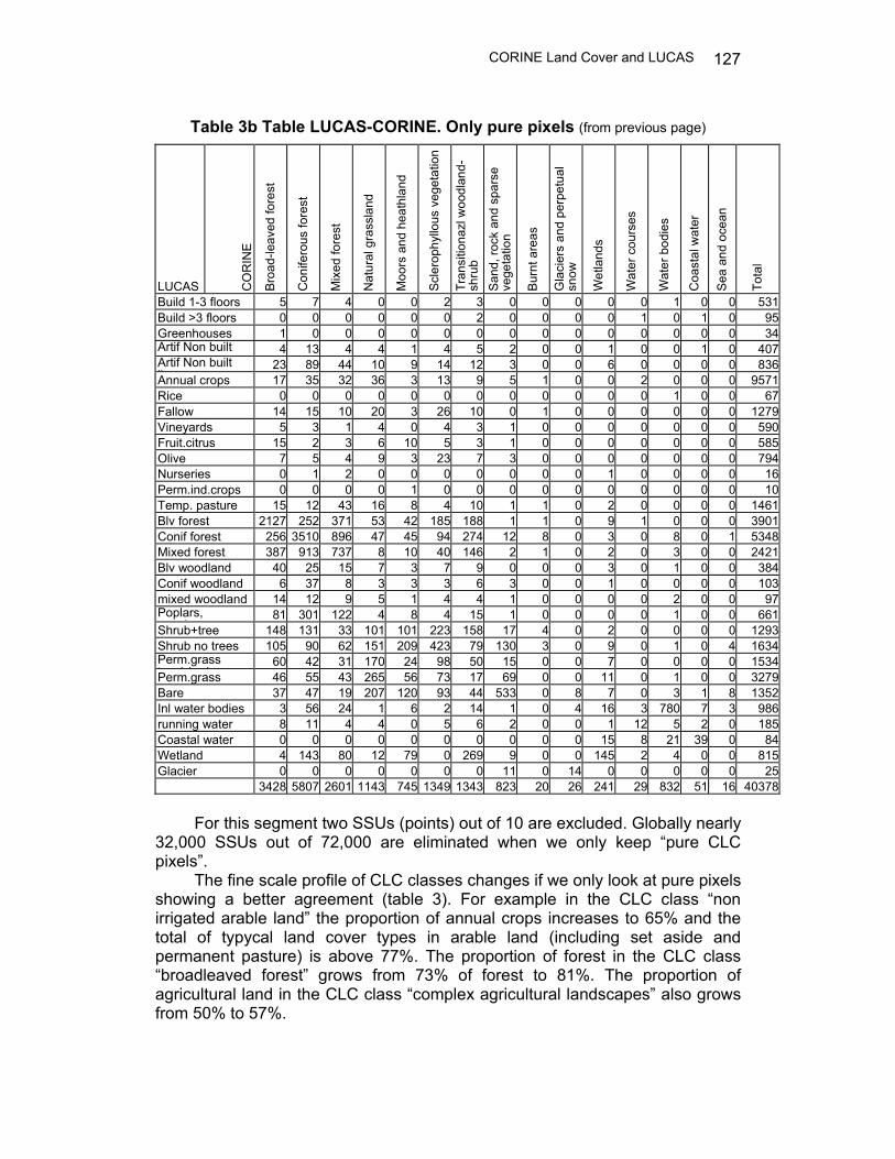
Table 3b Table LUCAS-CORINE. Only pure pixels (from previous page)

LUCAS CO

RIN

E

Broa

d-le

aved

fore

st

Con

ifero

us fo

rest

Mix

ed fo

rest

Nat

ural

gra

ssla

nd

Moo

rs a

nd h

eath

land

Scle

roph

yllo

us v

eget

atio

n

Tran

sitio

nazl

woo

dlan

d-sh

rub

Sand

, roc

k an

d sp

arse

ve

geta

tion

Burn

t are

as

Gla

cier

s an

d pe

rpet

ual

snow

Wet

land

s

Wat

er c

ours

es

Wat

er b

odie

s

Coa

stal

wat

er

Sea

and

ocea

n

Tota

l

Build 1-3 floors 5 7 4 0 0 2 3 0 0 0 0 0 1 0 0 531Build >3 floors 0 0 0 0 0 0 2 0 0 0 0 1 0 1 0 95Greenhouses 1 0 0 0 0 0 0 0 0 0 0 0 0 0 0 34Artif Non built 4 13 4 4 1 4 5 2 0 0 1 0 0 1 0 407Artif Non built li

23 89 44 10 9 14 12 3 0 0 6 0 0 0 0 836Annual crops 17 35 32 36 3 13 9 5 1 0 0 2 0 0 0 9571Rice 0 0 0 0 0 0 0 0 0 0 0 0 1 0 0 67Fallow 14 15 10 20 3 26 10 0 1 0 0 0 0 0 0 1279Vineyards 5 3 1 4 0 4 3 1 0 0 0 0 0 0 0 590Fruit.citrus 15 2 3 6 10 5 3 1 0 0 0 0 0 0 0 585Olive 7 5 4 9 3 23 7 3 0 0 0 0 0 0 0 794Nurseries 0 1 2 0 0 0 0 0 0 0 1 0 0 0 0 16Perm.ind.crops 0 0 0 0 1 0 0 0 0 0 0 0 0 0 0 10Temp. pasture 15 12 43 16 8 4 10 1 1 0 2 0 0 0 0 1461Blv forest 2127 252 371 53 42 185 188 1 1 0 9 1 0 0 0 3901Conif forest 256 3510 896 47 45 94 274 12 8 0 3 0 8 0 1 5348Mixed forest 387 913 737 8 10 40 146 2 1 0 2 0 3 0 0 2421Blv woodland 40 25 15 7 3 7 9 0 0 0 3 0 1 0 0 384Conif woodland 6 37 8 3 3 3 6 3 0 0 1 0 0 0 0 103mixed woodland 14 12 9 5 1 4 4 1 0 0 0 0 2 0 0 97Poplars,

l t81 301 122 4 8 4 15 1 0 0 0 0 1 0 0 661

Shrub+tree 148 131 33 101 101 223 158 17 4 0 2 0 0 0 0 1293Shrub no trees 105 90 62 151 209 423 79 130 3 0 9 0 1 0 4 1634Perm.grass t / h b

60 42 31 170 24 98 50 15 0 0 7 0 0 0 0 1534Perm.grass 46 55 43 265 56 73 17 69 0 0 11 0 1 0 0 3279Bare 37 47 19 207 120 93 44 533 0 8 7 0 3 1 8 1352Inl water bodies 3 56 24 1 6 2 14 1 0 4 16 3 780 7 3 986running water 8 11 4 4 0 5 6 2 0 0 1 12 5 2 0 185Coastal water 0 0 0 0 0 0 0 0 0 0 15 8 21 39 0 84Wetland 4 143 80 12 79 0 269 9 0 0 145 2 4 0 0 815Glacier 0 0 0 0 0 0 0 11 0 14 0 0 0 0 0 25 3428 5807 2601 1143 745 1349 1343 823 20 26 241 29 832 51 16 40378

For this segment two SSUs (points) out of 10 are excluded. Globally nearly

32,000 SSUs out of 72,000 are eliminated when we only keep “pure CLC pixels”.

The fine scale profile of CLC classes changes if we only look at pure pixels showing a better agreement (table 3). For example in the CLC class “non irrigated arable land” the proportion of annual crops increases to 65% and the total of typycal land cover types in arable land (including set aside and permanent pasture) is above 77%. The proportion of forest in the CLC class “broadleaved forest” grows from 73% of forest to 81%. The proportion of agricultural land in the CLC class “complex agricultural landscapes” also grows from 50% to 57%.


128

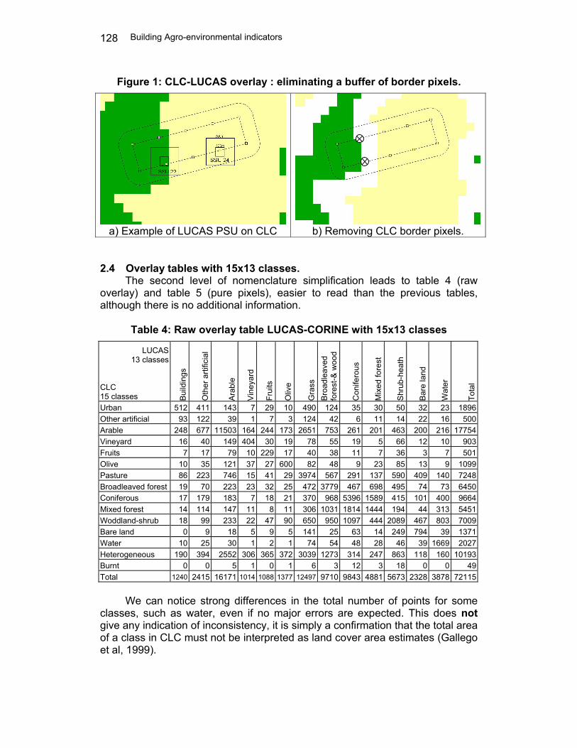
Figure 1: CLC-LUCAS overlay : eliminating a buffer of border pixels.

a) Example of LUCAS PSU on CLC

b) Removing CLC border pixels.

2.4 Overlay tables with 15x13 classes. The second level of nomenclature simplification leads to table 4 (raw

overlay) and table 5 (pure pixels), easier to read than the previous tables, although there is no additional information.

Table 4: Raw overlay table LUCAS-CORINE with 15x13 classes

LUCAS 13 classes

CLC 15 classes Bu

ildin

gs

Oth

er a

rtific

ial

Arab

le

Vine

yard

Frui

ts

Oliv

e

Gra

ss

Broa

dlea

ved

fore

st-&

woo

d

Con

ifero

us

Mix

ed fo

rest

Shru

b-he

ath

Bare

land

Wat

er

Tota

l

Urban 512 411 143 7 29 10 490 124 35 30 50 32 23 1896 Other artificial 93 122 39 1 7 3 124 42 6 11 14 22 16 500 Arable 248 677 11503 164 244 173 2651 753 261 201 463 200 216 17754 Vineyard 16 40 149 404 30 19 78 55 19 5 66 12 10 903 Fruits 7 17 79 10 229 17 40 38 11 7 36 3 7 501 Olive 10 35 121 37 27 600 82 48 9 23 85 13 9 1099 Pasture 86 223 746 15 41 29 3974 567 291 137 590 409 140 7248 Broadleaved forest 19 70 223 23 32 25 472 3779 467 698 495 74 73 6450 Coniferous 17 179 183 7 18 21 370 968 5396 1589 415 101 400 9664 Mixed forest 14 114 147 11 8 11 306 1031 1814 1444 194 44 313 5451 Woddland-shrub 18 99 233 22 47 90 650 950 1097 444 2089 467 803 7009 Bare land 0 9 18 5 9 5 141 25 63 14 249 794 39 1371 Water 10 25 30 1 2 1 74 54 48 28 46 39 1669 2027 Heterogeneous 190 394 2552 306 365 372 3039 1273 314 247 863 118 160 10193 Burnt 0 0 5 1 0 1 6 3 12 3 18 0 0 49 Total 1240 2415 16171 1014 1088 1377 12497 9710 9843 4881 5673 2328 3878 72115

We can notice strong differences in the total number of points for some

classes, such as water, even if no major errors are expected. This does not give any indication of inconsistency, it is simply a confirmation that the total area of a class in CLC must not be interpreted as land cover area estimates (Gallego et al, 1999).


129

Table 5: Overlay LUCAS-CORINE, pure pixels, 13x15 classes

LUCAS 13 classes

CLC 15 classes Bu

ildin

gs

Oth

er a

rtific

ial

Arab

le

Vine

yard

Frui

ts

Oliv

e

Gra

ss

Broa

dlea

ved

fore

st-&

woo

d

Con

ifero

us

Mix

ed fo

rest

Shru

b-he

ath

Bare

land

Wat

er

Tota

l

Urban 289 197 25 0 12 3 171 52 9 14 23 13 8 816 Other artificial 31 48 4 0 0 1 55 13 4 6 2 11 4 179 Arable 140 425 8926 94 147 90 1596 340 86 82 217 106 119 12368 Vineyard 11 24 79 263 15 11 28 19 8 2 28 8 2 498 Fruits 4 8 41 6 160 7 19 16 1 2 15 0 3 282 Olive 7 20 70 25 16 416 33 18 2 12 38 9 7 673 Pasture 33 109 308 5 17 10 2195 174 72 33 293 225 77 3551 Broadleaved forest 5 27 32 5 15 7 121 2248 262 401 253 37 15 3428 Coniferous 7 102 50 3 3 5 109 578 3547 925 221 47 210 5807 Mixed forest 4 48 42 1 5 4 117 508 904 746 95 19 108 2601 Woddland-shrub 7 45 64 7 19 33 340 461 425 205 1193 257 381 3437 Bare land 0 5 5 1 1 3 85 2 15 3 147 566 16 849 Water 3 8 3 0 1 0 21 15 13 7 16 19 1063 1169 Heterogeneous 85 177 1300 180 200 204 1383 501 95 79 379 60 57 4700 Burnt 0 0 2 0 0 0 1 1 8 1 7 0 0 20 Total 626 1243 10951 590 611 794 6274 4946 5451 2518 2927 1377 2070 40378

3 Discussion and possible ways forward. Contingency tables computed for all pixels are biased because of

mislocation: the profile of a CLC class includes pixels from neighbouring classes. The bias is likely in the sense of increasing apparent disagreement. Restricting contingency tables to pure pixels is expected to avoid jumping from one CLC class to another, but it may be biased in the opposite sense because more conflictive border areas are avoided. Now we try to tackle the next question: can we use the spatial structure of CLC to reduce the bias of the profile estimation?

3.1 Overlaying CLC and LUCAS: a possible formal scheme to deal with

co-location inaccuracy. Let us make a first simplification assuming that the territory is divided into

pixels of 1 ha. The information provided by LUCAS is a ground observation ( ) gjiL =, available for a sample of cells in row j and column i . CLC also gives

a value for each cell ( ) cjiC =, The location accuracy requested in LUCAS is of the order of a few meters,

better than the 100 m. location accuracy requested to CLC, therefore we take the orthophotos used for LUCAS as reference geometry and we consider the location error of CLC by writing the observation as ( ) ( ) cjiCjiC ′=′′=′ ,, , where

1ε+=′ ii ; 2ε+=′ jj . 1ε and 2ε are the vertical and horizontal location error, that we assume for the moment within the CLC specifications (100 m maximum error) and isotropic (i.e. the same in any direction):


130

( ) ( )

−=

−==

qq

qpp 21

101

21 εε

where we generally expect a parameter 3/1<q (the probability of staying in the same pixel is higher than the probability of jumping to each of the neighbouring pixels).

Under this assumption table 6 shows the probability scheme of the apparent location of a LUCAS point that would fall on the central cell of the table.

Table 6 : Mislocation probability scheme

2q ( )qq 21− 2q

( )qq 21− ( )221 q− ( )qq 21−

2q ( )qq 21− 2q

We call H the GIS overlay matrix:

( ) ( )( )cjiCgjiLH cg =′== ,,,#,

cgH ,1 is the overlay matrix restricted to the 1 ha pixels that are CLC-pure, i.e. surrounded by pixels of the same CLC class. cgH ,2 is the overlay matrix for the CLC border pixels. The marginals and conditional proportions are:

∑=+g

cgc HH , ∑=+g

cgc HH ,11 ∑=+g

cgc HH ,22

( )c

cg

HH

cgH,

,/+

= ( )c

cg

HH

cgH,

,

11

/1+

= ( )c

cg

HH

cgH,

,

22

/2+

=

The confusion matrix A is the overlay matrix that would have been obtained without location error, i.e assuming ( ) ( )jiCjiC ,, =′ :

( ) ( )( )cjiCgjiLA cg === ,,,#,

Notice that even with location errors the marginals cA ,+ cA ,1+ and cA ,2+ coincide with those of the overlay matrix H (the total number of pixels with each CLC class).

Our target is estimating the proportion of each ground class g in each CLC class c , i.e. the conditional proportions associated to the overlay matrix:


131

( )c

cg

AA

cgA,

,/+

=

In order to make the link between the confusion matrix A and the overlay matrices G , 1G , and 2G , we need to consider the number of cases in which mislocation causes jumping from class c to class c′ . Let us call ( )ccB ′,1 the number of pairs of contiguous pixels (with a common side) with CLC classes c and c′ . ( )ccB ′,2 is the number of pairs of corner-contiguous pixels (with a common corner) with CLC classes c and c′ . According to the model specified in table 7 the probability that mislocation causes a jump from class c to class c′ is:

( ) ( )[ ] ( ) ( )( )

( )( )+

′+

+−′

==′=′,2,2

,121,1,/,

2

cBqccB

cBqqccBcjiCcjiCp

Under this model, we are sure that the cgH ,1 pure pixels did not change CLC class by mislocation, While the cgH ,2 border can actually come from the same class or from other classes. The expected confusion matrix is

[ ] ( ) ( ) ( )[ ] cgc

cgcgcg HcjiCcjiCpHpHAE ,'

,21,, 2,/,201 ∑ =′=′+==+= εε

( ) ( ) ( )( )

( )( )∑

′′+

′+

+−′

+−+=c

cgcgcg HcBqccB

cBqqccBHqH ,

2

,2

, 2,2,2

,121,12211

Because of the very large number of CLC pixels, [ ]cgAE , can be approximately identified with cgA , . 1H , 2H are known. 1B and 2B can be computed from CLC, but q has to be estimated.

A reliable estimation of q would require knowing the distribution of the co-location inaccuracy. Alternatively some indirect method could be designed using the comparison of 1H and 2H , but this would require additional hypothesis. This problem remains anyway out of the scope of this paper.

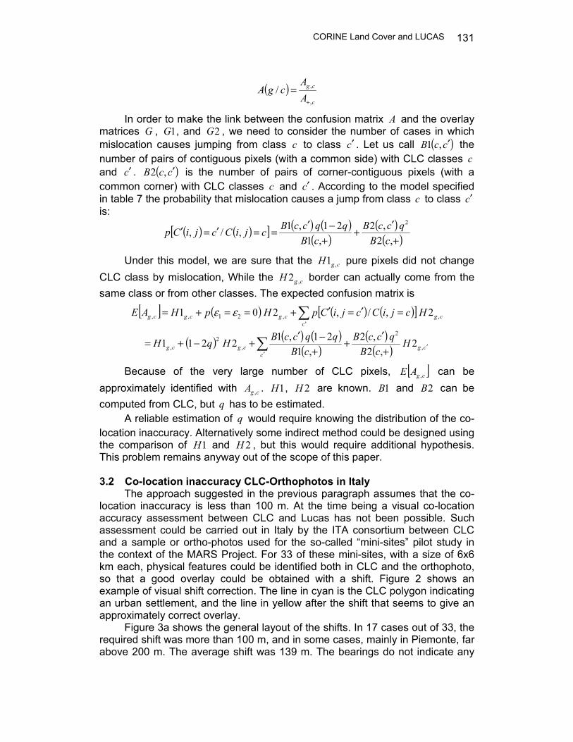
3.2 Co-location inaccuracy CLC-Orthophotos in Italy

The approach suggested in the previous paragraph assumes that the co-location inaccuracy is less than 100 m. At the time being a visual co-location accuracy assessment between CLC and Lucas has not been possible. Such assessment could be carried out in Italy by the ITA consortium between CLC and a sample or ortho-photos used for the so-called “mini-sites” pilot study in the context of the MARS Project. For 33 of these mini-sites, with a size of 6x6 km each, physical features could be identified both in CLC and the orthophoto, so that a good overlay could be obtained with a shift. Figure 2 shows an example of visual shift correction. The line in cyan is the CLC polygon indicating an urban settlement, and the line in yellow after the shift that seems to give an approximately correct overlay.

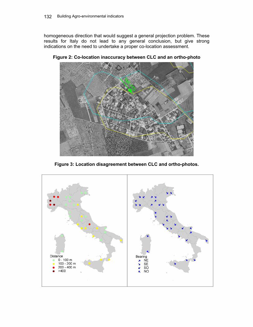
Figure 3a shows the general layout of the shifts. In 17 cases out of 33, the required shift was more than 100 m, and in some cases, mainly in Piemonte, far above 200 m. The average shift was 139 m. The bearings do not indicate any


132

homogeneous direction that would suggest a general projection problem. These results for Italy do not lead to any general conclusion, but give strong indications on the need to undertake a proper co-location assessment.

Figure 2: Co-location inaccuracy between CLC and an ortho-photo

Figure 3: Location disagreement between CLC and ortho-photos.


133

3.3 Can LUCAS be used to assess the accuracy of CLC? Assessing the thematic accuracy of geographic information is more

complex than evaluating the geometric accuracy. Standard criteria are difficult to establish and a large scientific literature on the issue has been produced in the last 20 years (Lowell and Jaton, 1999, Mowrer and Congalton, 1999). There is still much to do from the methodological point of view, in particular for the case of land cover information.

When two land cover information layers are available for the same area and one of them is assumed to be more precise, an indicator of the agreement between both can be seen as an accuracy measure of the less precise layer.

The more precise layer is usually known only for a sample, and improved information may be obtained combining it with less precise but exhaustive information. This is the case of CLC and Lucas.

The disagreement between two layers can be thematic, i.e. different land cover types are reported by both layers for the same area, but it can come as well from a co-location problem. Thematic disagreements can come from an error (in principle of the layer assumed to be less precise), from differences in the classification nomenclature, from different scales or from different reference dates. Co-location inaccuracy may be due to mislocation in the data collection (systematic shift for example), or to further manipulation (co-ordinates projection, elaboration of mosaics, reference geoid, etc).

The complex problem of measuring thematic inaccuracy or disagreement becomes easier to manage if we assume that there is no co-location error, the reference date and the scale are the same and both layers have the same nomenclature. Under these implicit assumptions several agreement indicators can be computed such as the kappa index (Congalton and Green, 1999).

Unfortunately these simplification assumptions are far from being acceptable when CLC and LUCAS data are overlaid: co-location inaccuracy is not negligible, scale and reference dates are substantially different, and nomenclature criteria are necessarily different, since the targets and scales are different. The confusion matrices and disagreement indicators reported below cannot be directly interpreted as an indication of errors in CLC.

If we read the overlay tables given above as accuracy measures and we compute indexes, the results may be worrying at first sight, but a more nuanced discussion is needed.

For example a previous assessment of CLC in Arezzo (Italy) shows that the values of accuracy indicators computed by straightforward overlay can be drastically distorted by the effect of scale (Gallego, 2001). In the Arezzo study two land cover maps at different scales were compared; co-location and nomenclature problems were minimal, still a simple pixelwise overlay gave low values for agreement indicators, but after removing the scale effect, the agreement became satisfactory except for the class “pasture”, with a minor presence in that test site. The conclusions of this study might be specific for the Arezzo test site, but the warning about negative distortions of agreement indicators has a general validity.

When CLC and Lucas are compared, besides the different scales, we have indications of possible strong co-location inaccuracy and significant nomenclature differences. Therefore the negative distortion of agreement


134

indicators can be very high. A major step to improve the interpretation of such indicators is assessing the possible co-location inaccuracy. This can be done by selecting a subsample of LUCAS PSUs (Primary Sampling Units) for which the shift may be visually identified. This can be done if there are objects that can be identified both in CLC and in the ortho-photos used as ground survey documents for Lucas. It is difficult to determine a priori if it will be possible do identify common objects in CLC and an ortho-photo, but some hints can be given by the presence of CLC categories usually easier to identify, such as water. In any case a basic condition for the feasibility of co-location accuracy assessment is the availability of the ortho-photos used for LUCAS ground work.

Because of the different scales of CLC and LUCAS, nearly any combination of classes is possible without any thematic error, so that a certain amount of disagreement is perfectly normal. If one point is forest in LUCAS and arable land in CLC, there is a disagreement, although this does not mean that there is an error. If there is a disagreement in 2 points out of 10 in a LUCAS Primary Sampling Unit (PSU), there is no significant indication of thematic inaccuracy, but suspicions appear if more than 5 points are in disagreement.

Beyond the question of scale, it is sometimes difficult to decide if a certain combination of classes can be considered to be fully in agreement or in disagreement. For example the CLC class 311=”broad-leaved forest” is not in fully agreement with the LUCAS class C23=”mixed wooded area”, but the level of disagreement is not the same as with LUCAS G01=”inland water bodies”.

This suggests the introduction of intermediate levels of disagreement, corresponding to some degree of compatibility (Congalton and Green, 1999). Table 6 illustrates a possible definition. A value 0=ijϕ means disagreement, a value 1=ijϕ means complete agreement and intermediate values correspond to different levels of agreement. Some CLC classes, such as 2.4.2 “complex cultivation patterns” are more or less in agreement with almost any Lucas class, but the level is not necessarily the same. The definition given by table 6 is certainly subjective and needs to be discussed.

A traditional synthetic agreement indicator is the kappa index (Bishop et al, 1975):

ii

i

ii

ii

ii

pp

pppK

++

++

∑∑∑

−

−=

1

The kappa index has a value 0 if the agreement is the same that would be obtained at random, and a value 1 if the agreement is perfect. The application of the kappa index assumes that the nomenclature is the same in both layers and any pair of non-coinciding classes is a complete disagreement. To adapt the kappa index to a fuzzy disagreement scheme, we can write,

( )∑

∑++

++

−

−=′

ijjiij

jiijij

ij

pp

pppK

ϕ

ϕ

1


135

Table 7: Example of fuzzy agreement definition

LUCAS 13 classes

CLC 15 classes Bu

ildin

gs

Oth

er a

rtific

ial

Arab

le

Vine

yard

Frui

ts

Oliv

e

Gra

ss

Broa

dlea

ved

fore

st &

-woo

d

Con

ifero

us

Mix

ed fo

rest

Shru

b-he

ath

Bare

land

Wat

er

Urban 1 0.7 0 0 0 0 0.5 0.3 0.3 0.3 0 0.3 0.1 Other artificial 0.7 1 0 0 0 0 0.5 0 0 0 0 0.5 0 Arable 0 0 1 0 0 0 0.7 0 0 0 0 0 0 Vineyard 0 0 0 1 0 0 0 0 0 0 0 0 0 Fruits 0 0 0 0 1 0 0 0 0 0 0 0 0 Olive 0 0 0 0 0 1 0 0 0 0 0 0 0 Pasture 0 0 0.3 0 0 0 1 0.2 0.2 0.2 0.2 0 0 Broadleaved forest 0 0 0 0 0 0 0 1 0.2 0.7 0.3 0 0 Coniferous 0 0 0 0 0 0 0 0.2 1 0.7 0.3 0 0 Mixed forest 0 0 0 0 0 0 0 0.8 0.8 1 0.3 0 0 Woddland-shrub 0 0 0 0 0 0 0 0.8 0.8 0.8 1 0 0 Bare land 0 0 0 0 0 0 0 0 0 0 0 1 0 Water 0 0 0 0 0 0 0 0 0 0 0 0 1 Heterogeneous 0.5 0.5 0.5 0.5 0.5 0.5 0.5 0.5 0.5 0.5 0.5 0.5 0.5 Burnt 0 0 0.3 0.3 0.3 0.3 0.3 0.8 0.8 0.8 0.8 0.5 0

This adapted kappa index also ranges between 0 for random attribution

and 1 for perfect agreement. The value of the “fuzzy kappa” index for the raw Table 4 with the definition given in Table 7 is 0.502, while for the “pure pixels” (Table 5), the value reaches 0.590.

4 Conclusions The matrices obtained from a GIS overlay of CLC and LUCAS have a rich

information, but its interpretation in terms of CLC accuracy is hazardous because many sources of disagreement are confounded. Computing fine scale profiles of CLC classes is feasible, but a better knowledge of the distribution of the co-location inaccuracy is needed in order to estimate the probability of jumping between raster cells.

The situation will improve when CLC2000 is available, although the co-location problems will never disappear completely. A formal model is outlined that may be applied in the future when such co-location inaccuracy is sufficiently known. This target can be achieved by a visual comparison of a sub-sample of LUCAS Primary Sampling Units (PSU’s) on CLC and on the ortho-photographs used as ground documents for LUCAS.

This research indicates that the direct use of LUCAS to assess the thematic accuracy of CLC2000 is not adequate, but an enhanced photo-interpretation of LUCAS PSUs can provide a good assessment. A fuzzy disagreement matrix might provide a useful tool for computing a numerical accuracy indicator.


136

Acknowledgements

We are grateful to the ITA consortium, and in particular to Paolo Ragni, Aldo Giovacchini and Francesco Lucarelli for the information and figures provided on the co-location problems in Italy. Stefano Bagli has checked the results of GIS overlays. Bob Jones gave useful suggestions to improve the paper.

References Bishop Y., Fienberg S., Holland P., 1975, Discrete Multivariate Analysis, M.I.T.

press, Cambridge, Ma. CEC, 1993, CORINE Land Cover; guide technique, Report EUR 12585EN.

Office for Publications of the European Communities. Luxembourg,. 144 pp Congalton R.G., Green K., 1999, Assessing the accuracy of remotely sensed

data: principles and practices, Lewis publishers. 137 pp. Delincé J., 2001, A European approach to area frame survey. Proceedings of

the Conference on Agricultural and Environmental Statistical Applications in Rome (CAESAR), June 5-7, Vol. 2 pp. XXV.1-10.

Gallego J., 2001, Comparing CORINE Land Cover with a more detailed database in Arezzo (Italy). Towards Agri-environmental indicators, Topic report 6/2001 European Environment Agency, Copenhagen, pp. 118-125.

Gallego, F.J. Carfagna, E., Peedell S., 1999, The use of CORINE Land Cover to improve area frame survey estimates in Spain. Research in Official Statistics, Vol 2, no 2, pp. 99-122

Kayadjanian M., Vidal C., 2001, Reassignment of the farm structure survey’s data. Towards Agri-environmental indicators, Topic report 6/2001 European Environment Agency, Copenhagen, pp. 75-91. gs-Crouzet Ph., Steenmans Ch., Agricultural statistics spatialisation by means of CORINE Land Cover to model nutrient surpluses. Towards Agri-environmental indicators, Topic report 6/2001 European Environment Agency, Copenhagen, pp. 104-115.

Lowell K., Jaton A. (ed), 1999, Spatial Accuracy assessment: Land information uncertainty in natural resources, Ann Arbor Press, Chelsea, Michigan, USA. 443 pp.

Mowrer H.T., Congalton, R.G. (Ed.), 1999, Quantifying Spatial Uncertainty in Natural Resources: Theory and Applications for GIS and Remote Sensing. Ann Arbor Press, Chelsea, Michigan, USA. 235 pp.

Perdigão V., Annoni A., 1997, Technical and methodological guide for updating CORINE Land Cover data base. Report EUR 17288 EN. Office for Publications of the European Communities. Luxembourg,. 124 pp

fine scale profile of corine land cover classes with...

Documents