Finding Tours in the TSP

David ApplegateComputational and Applied MathematicsRice University

Robert BixbyComputational and Applied MathematicsRice University

Va�sek Chv�atalDepartment of Computer ScienceRutgers University

William Cook�

Computational and Applied MathematicsRice University

ABSTRACT

The traveling salesman problem, or TSP for short, is easy to state:given a �nite number of \cities" along with the cost of travel betweeneach pair of them, �nd the cheapest way of visiting all the cities andreturning to your starting point. The travel costs are symmetric in thesense that traveling from city X to city Y costs just as much as travel-ing from Y to X; the \way of visiting all the cities" is simply the orderin which the cities are visited. In this report we consider the relaxedversion of the TSP where we ask only for a tour of low cost. This is apreliminary version of a chapter of planned monograph on the TSP.

�Supported by ONR Grant N00014-98-1-0014.

C H A P T E R 2

Finding Tours

2.1 INTRODUCTION

In this chapter we consider the relaxed version of the TSP where we ask onlyfor a tour of low cost. This task is much easier, but performing it well is animportant ingredient in a branch and bound search method for the TSP, aswell as being an interesting problem in its own right. Indeed, tour �nding is amore popular topic than the TSP itself, having a large and growing literaturedevoted to its various aspects. Our study will be restricted to the narrow �eldof tour �nding that is applicable to solution methods for the TSP, namely,�nding near-optimal tours within a reasonable amount of computing time.Other tour-�nding topics (in particular, �nding good tours very quickly) canbe found in Bentley [1992], Johnson [1990], Johnson, Bentley, McGeoch, andRothberg [1998], Johnson and McGeoch [1997], and Reinelt [1994].

2.2 LIN-KERNIGHAN

At the heart of the most successful tour-�nding approaches to date lies thesimple and elegant algorithm of Lin and Kernighan [1973]. This is remarkable,given the wide range of attacks that have been made on the TSP in the pasttwo decades, and even more so when one considers that Lin and Kernighan'sstudy was limited to problem instances having at most 110 cities (very smallexamples by today's standards). We begin by describing brie y some of thework leading up to their approach.

Shortly after the publication of Dantzig, Fulkerson, and Johnson's [1954]classic paper, Flood [1956] studied their 49-city example from a tour-�ndingperspective. He began by solving the assignment problem relaxation to the

1

2 FINDING TOURS

TSP, obtaining the dual solution (u0; : : : ; u48). He used these values to com-pute a reduced cost matrix [cij ] by subtracting ui + uj from the original costof travel for each pair of cities (i; j). (Note that this does not alter the setof optimal solutions to the TSP, but it may help in �nding a good tour.)Working with these costs, Flood found a nearest neighbor tour by choosing astarting city (in his case, Washington, D.C.) and then always proceeding tothe closest city that was not already visited. He followed this with a localimprovement phase, making use of the observation that in any optimal tour,(i0; : : : ; in�1), for an n-city TSP, for each 0 � p < q < n (subscripts will betaken modulo n) we have

cip�1ip + ciqiq+1 � cip�1iq + cipiq+1 : (2.1)

A pair (p; q) that violated (2.1) was called an \intersecting pair", and hismethod was to �x any such pair until the tour became \intersectionless".

Croes [1958] used Flood's intersectionless tours as a starting point for anexhaustive search algorithm for the TSP. He also described a procedure for�nding an intersectionless tour by a sequence of \inversions". The observationis that if (p; q) intersect in the tour

(i0; : : : ; ip�1; ip; : : : ; iq ; iq+1; : : : ; in�1);

then the pair can be �xed by inverting the subsequence (ip; : : : ; iq), that is,moving to the tour

(i0; : : : ; ip�1; iq ; iq�1; : : : ; ip+1; ip; iq+1; : : : ; in�1):

We call this operation ip(p; q). (We assume that tours are oriented, soflip(p; q) is well-de�ned.)

A strengthening of Croes' inversion method was proposed and tested byLin [1965]. (See also Morton and Land [1955] and Bock [1958].) Rather thansimply ipping a subsequence (ip; : : : ; iq), he also considered reinserting it(either as is, or ipped) between two other cities that are adjacent in thetour, if such a move would result in a tour of lesser cost. This increases thecomplexity of the algorithm, but Lin showed that it produces much bettertours. (Reiter and Sherman [1965] studied a similar method, but includeda speci�c recipe for which subsequences to consider and allowed arbitraryreorderings of the subsequence, rather than just ips.)

Lin [1965] also provided a common framework for describing intersectionlesstours and tours that are optimal with respect to ips and insertion. He calleda tour �-optimal if it is not possible to obtain a tour of lesser cost by replacingany � of its edges (considering the tour as a cycle in a graph) by any otherset of � edges. Thus, a tour is intersectionless if and only if it is 2-optimal.Moreover, it is not di�cult to see that a tour is optimal with respect to ips and insertion if and only if it is 3-optimal. Croes' algorithm and Lin'salgorithm are commonly referred to as 2-opt and 3-opt, respectively.

LIN-KERNIGHAN 3

A natural next step would be to try �-opt for some greater values of �,but Lin found that despite the greatly increased computing time for 4-opt,the tours produced were not noticeably better than those produced by 3-opt.As an alternative, Lin and Kernighan [1973] developed an algorithm thatis sometimes referred to as \variable �-opt". The core of the algorithm isan e�ective search method for tentatively performing a (possibly quite long)sequence of ips such that each initial subsequence appears to have a chance ofleading to a tour of lesser cost. (It may help in understanding their algorithmto note that while any �-opt move can be realised as a sequence of ips,some of the intermediate tours may have cost greater than that of the initialtour, even in an improving �-opt move.) If the search is successful in �ndingan improved tour, then the sequence of ips is made and a new search isbegun. Otherwise, the tentative ips are discarded before we begin a newsearch, and we take care not to repeat the same unsuccessful sequence. Theprocedure terminates when every starting point for the search has proven tobe unsuccessful.

We now describe the search method. The algorithm we present di�ersfrom the one given in Lin and Kernighan [1973], but the essential ideas arethe same. We describe the method in su�cient detail to have a basis fordiscussing our computational study in later sections.

Suppose we are given a TSP with c(i; j) representing the cost of travelbetween vertex i and vertex j. Let T be a tour and let base be a selectedvertex. We will build a sequence of ip operations, and denote by current tourthe tour obtained by applying the ip sequence to T . For any vertex v, letnext(v) denote the vertex that comes immediately after v in current tour

and let prev(v) denote the vertex that comes immediately before v. (Sincea tour is oriented, next and prev are well-de�ned.) The only ips that willbe considered are those of the form flip(next(base); probe), for vertices probethat are distinct from base, next(base), and prev(base). Such a ip willreplace the edges (base; next(base)) and (probe; next(probe)) by the edges(next(base); next(probe)) and (base; probe). (See Figure 2.1.) current tour

would be improved by such a ip if and only if

c(base; next(base)) + c(probe; next(probe)) > (2.2)

c(next(base); next(probe)) + c(base; probe);

as in the 2-opt algorithm. Rather than demanding such an improving ip,Lin-Kernighan requires that

c(base; next(base))� c(next(base); next(probe)) > 0:

This is a greedy approach that trys to improve a single edge in the tour. Theidea can be extended as follows. Let delta be a variable that is set to 0 at thestart of the search and is incremented by

c(base; next(base))� c(next(base); next(probe)) +

4 FINDING TOURS

next(probe) probeprobe

base next(base) base

Figure 2.1. flip(next(base); probe))

c(prob; next(probe))� c(probe; base)

after each flip(next(base); probe)). Thus, delta represents the amount of localimprovement we have obtained thus far with the sequence of ips. (The costof current tour can be obtained by subtracting delta from the cost of thestarting tour T .) In a general step, we require that

delta+ c(base; next(base))� c(next(base); next(probe)) > 0: (2.3)

Thus, we permit delta to be negative, as long as it appears that we might beable to later realize an improvement. We call probe a promising vertex if (2.3)holds.

A rough outline of the search method can be summarized as follows:

delta = 0while there exist promising verticesdo choose a promising vertex probe

delta = delta+ c(base; next(base))� c(next(base); next(probe))+c(probe; next(probe)) � c(probe; base)

add flip(next(base); probe)) to the ip sequenceend.

If we reach a cheaper tour, we record the sequence of ips, but continue onwith the search to see if we might �nd an even better tour.

Notice that probe is promising if and only if the cost of the edge

(next(base); next(probe))

is small enough. (The other two terms in (2.3) do not depend on probe.) So ane�cient way to check for a promising vertex is to consider the edges incidentwith vertex next(base), ordered by increasing costs. When we consider edge(next(base); a), we let probe = prev(a). See Figure 2.2.

Just selecting the �rst edge that produces a promising probe is too short-sighted and often leads to long sequences that do not result in better tours.

LIN-KERNIGHAN 5

probe = prev(a)

next(base)base

a

Figure 2.2. Finding a promising vertex

Instead, Lin-Kernighan also considers a third term from (2.2), choosing theedge (next(base); a) that maximizes

c(prev(a); a)� c(next(base); a): (2.4)

To avoid computing this quantity for all edges incident with next(base), onlya prescribed subset of vertices a are considered. We refer to this prescribedsubset as the set of neighbors of a vertex. (A typical example of a neighbor setis the set of k closest vertices, for some �xed integer k.) The price we pay forusing only the neighbors of next(base) is that we may overlook a promising ip operation. This is outweighed, however, by the greatly reduced time ofthe steps in the search. We call a neighbor, a, of next(base) promising ifprobe = prev(a) is a promising vertex. The outline of the search becomes:

delta = 0while there exist promising neighbors of next(base)do let a be the promising neighbor of next(base) that

maximizes (2.4)delta = delta+ c(base; next(base))� c(next(base); a) +

c(prev(a); a) � c(prev(a); base)add flip(next(base); prev(a))) to the ip sequence

end.

To increase the chances of �nding an improving sequence, a limited amountof backtracking is used. For each integer k � 1, let breadth(k) be the maxi-mum number of promising neighbors we are willing to consider at level k of thesearch. Rather than just adding the ip involving the most promising neigh-bor, we will consider, separately, adding the ips involving the breadth(k)promising neighbors having the greatest values of (2.4). (Lin and Kernighanset breadth(1) = 5, breadth(2) = 5, and breadth(k) = 1 for all k > 2. Settingbreadth(k) = 0 for some k provides an upper bound on the length of any ipsequence that will be considered.)

Mak andMorton [1993] proposed another method for increasing the breadthof a search. Their idea is to try ips of the form flip(probe; base), as well as

6 FINDING TOURS

those that we normally consider. This can be accomplished by consideringthe neighbors a of base (other than next(base) and prev(base)), that satisfy

delta+ c(base; next(base))� c(base; a) > 0:

In this case, the vertices are ordered by decreasing values of

c(a; next(a))� c(base; a) (2.5)

and after a flip(next(a); base), the value of delta is incremented by

c(base; next(base))� c(base; a) + c(a; next(a))� c(next(a); next(base)):

These details are analogous to those for the usual ips. The �nal piece of aMak-Morton move is to change base to be the vertex that was next(a) beforethe ip. This means that next(base) is the same vertex before and after the ip, analogous to the fact that base remains the same in the usual case. SeeFigure 2.3.

a

base next(base) next(base)

next(a) base

a

Figure 2.3. A Mak-Morton move

There is no need to consider the Mak-Morton moves separately from theusual ips, so we can create a single ordering consisting of the permittedneighbors of next(base) and base, sorted by non-increasing values of (2.4)and (2.5), respectively. (Some vertices may appear twice in the ordering.)Call this the lk�ordering for base. At each step of the search, the verticeswill be processed in this order.

To give an outline of the full search routine (incorporating backtrackingand Mak-Morton moves), it is convenient to use the recursive function step

de�ned in Algorithm 2.1. This function takes as arguments the current leveland the current delta. A search from base is then just a call to step(1,0).Note again that at any point, the cost of current tour can be computed usingthe cost of the initial tour and delta. It is easy, therefore, to detect when animproved tour has been found.

Lin-Kernighan increases the breadth of a search in a third way, by consid-ering an alternative �rst step. The usual flip(next(base); prev(a)) removes

LIN-KERNIGHAN 7

create the lk�ordering for basei = 1while there exist unprocessed vertices in the lk�ordering

and i �breadth(level)do let a be the next vertex in the lk�ordering

if a is speci�ed as part of a Mak-Morton movethen g = c(base; next(base))� c(base; a)+

c(a; next(a))� c(next(a); next(base))newbase = next(a)oldbase = base

add flip(newbase; base) to the ip sequencebase = newbase

call step(level+ 1; delta+ g)base = oldbase

else g = c(base; next(base))� c(next(base); a) +c(prev(a); a)� c(prev(a); base)

add flip(next(base); prev(a)) to the ip sequencecall step(level+ 1; delta+ g)

endif an improved tour has been found, then RETURNelse delete the added ip from the end of the

ip sequenceincrement i

endend.

Algorithm 2.1. step(level, delta)

8 FINDING TOURS

the edge (prev(a); a) from the tour. The alternative (actually a sequence of ips) will remove (a; next(a)). To accomplish this, we select a neighbor b

of next(a). There are two cases, depending on whether or not b lies on thesegment of the tour from next(base) to a. If b lies on this segment, then twosequences of ips are considered, the �rst removes (b; next(b)) from the tourand the second removes (prev(b); b) from the tour. These moves are illustrated

flip(s1, a), flip(b, s1), flip (a, b1)

basebase s1 = next(base)

basebase s1 = next(base)

a1 = next(a) a

b1 = next(b)

b

a

b

aa1 = next(a)

b

b1 = prev(b)

a

b

flip(s1, b), flip(b, a)

Figure 2.4. Alternative �rst step, case 1

in Figure 2.4, together with the ips needed to realize them. If b does not lieon the segment from next(base) to a, then we select a neighbor d of prev(b),such that d lies on the segment from next(base) to a. We again consider twosequences of ips, the �rst removing (d; next(d)) and the second removing(prev(d); d). These moves are illustrated in Figure 2.5.

To permit backtracking in this alternate �rst step, let breadthA be themaximum number of vertices a that we are willing to try, let breadthB bethe maximum number of pairs (b; b1) (where b1 is either next(b) or prev(b)),and let breadthD be the maximum number of pairs (d; d1) (where d1 is eithernext(d) or prev(d)). In selecting a, we consider only the promising neigh-bors of next(base). These are ordered by decreasing value of c(next(a); a) �c(next(base); a). Call this the A�ordering. In selecting (b; b1), we considerthe neighbors of next(a), distinct from base, next(base), and a, that satisfy

c(next(a); b) < c(a; next(a)) + c(base; next(base))� c(next(base); a):

LIN-KERNIGHAN 9

a1 = next(a)

basebase s1 = next(base)

d d

basebase s1 = next(base)

d

d1 = next(d)

d

d1 = prev(d)

a

b

a

b

a a

bb

flip(s1, b1), flip(b1, d1), flip(a1, s1)

flip(s1, d1), flip(d, a), flip(a1, b1)

a1 = next(a)

b1 = prev(b)

b1 = prev(b)

Figure 2.5. Alternative �rst step, case 2

(This is the analogue of inequality (2.3).) The pairs are ordered by decreasingvalues of c(b1; b)� c(next(a); b). Call this the B�ordering. Finally, in select-ing (d; d1), we consider the neighbors of b1, distinct from base, next(base), a,next(a), and b, that satisfy

c(b1; d) < c(b; b1) + c(base; next(base)� c(next(base); a)

+ c(a; next(a)) � c(next(a); b):

In this case, the pairs are ordered by decreasing values of c(d1; d) � c(b1; d).Call this the D�ordering.

With this terminology, we can write the function alternate step as inAlgorithm 2.2.

10 FINDING TOURS

s1 = next(base)create the A�ordering of the neighbors of next(base)i = 1while there exist unprocessed vertices in the A�ordering and

i � breadthAdo let a be next vertex in the A�ordering

a1 = next(a)create the B�ordering from the neighbors of next(a)j = 1while there exists unprocessed pairs in the B�ordering and

j � breadthBdo let (b; b1) be the next pair in the B�ordering

if b lies of the tour segment from next(base) to a

then add the ips listed in Figure 2.4 to the ip sequenceand set delta to the di�erence of the weight of thedeleted edges and the weight of the added edgescall step(3, delta)if an improved tour has been found, then RETURNelse delete the added ips from the ip sequence

else create the D�ordering from the neighbors of b1k = 1while there exist unprocessed pairs in the

D�ordering and k � breadthDdo let (d; d1) be the next pair in the D�ordering

add the ips listed in Figure 2.5 to the ipsequence and set delta as abovecall step(4, delta)if an improved tour has been foundthen RETURNelse delete the added ips from the

ip sequenceincrement k

endend

endincrement j

endincrement i

end.

Algorithm 2.2. alternate step

LIN-KERNIGHAN 11

Putting the pieces together, we can write the function lk search, thattakes as arguments a vertex v and a tour T , as in Algorithm 2.3.

initialize current tour as Tinitialize an empty ip sequencebase = v

call step(1, 0)if an improved current tour has been foundthen RETURN the improving ip sequenceelse call alternate step()

if an improved current tour has been foundthen RETURN the improving ip sequenceelse RETURN with an unsuccessful ag

end.

Algorithm 2.3. lk search(v, T )

To apply this, we mark all vertices, then call lk search(v) for some ver-tex v. If the search is unsuccessful, we unmark v and continue with someother marked vertex. If the search is successful, then it is possible that someunmarked vertices may now permit successful searches. For this reason, Linand Kernighan again mark all vertices before continuing with the next search.This was an appropriate strategy for the problem instances they studied, butit is too time consuming for larger instances. The trouble is that unmarkedvertices that are not close to the improving sequence of ips have little chanceof permitting successful searches. To deal with this issue, Bentley [1990] (inthe context of 2-opt), proposed to mark only those vertices that are the endvertices of one of the ips in the improving sequence. This leads to somewhatworse tours, but greatly improves the running time of the algorithm. We sum-marize the method in the function lin kernighan described in Algorithm 2.4;lin kernighan takes as an argument a tour T .

The Lin-Kerngihan routine consistently produces good quality tours on awide variety of problem instances. Computational results on variations of thealgorithm can be found in Bachem and Wottawa [1992], Bland and Shall-cross [1989], Codenotti, Manzini, Margara, and Resta [1996], Gr�otschel andHolland [1991], Johnson [1990], Johnson and McGeoch [1997], J�unger, Reinelt,and Rinaldi [1995], Mak and Morton [1993], Padberg and Rinaldi [1991], Pert-tunen [1994], Reinelt [1994], Rohe [1997], Sch�afer [1994], Verhoeven, Aarts,

12 FINDING TOURS

initialize lk tour as Tmark all verticeswhile there exist marked verticesdo select a marked vertex v

call lk search(v, lk tour)if an improving sequence of ips is foundthen while the ip sequence is nonempty

do let flip(x; y) be the next ip in the sequenceapply flip(x; y) to lk tour to obtain a newlk tour

mark vertices x and y

delete flip(x; y) from the ip sequenceend

else unmark v

endRETURN tour lk tour.

Algorithm 2.4. lin kernighan(T )

van de Sluis, and Vaessens [1995], Verhoeven, Swinkels, and Aarts [1995], aswell as the original paper of Lin and Kernighan [1973].

An important part of Lin and Kernighan's overall tour-�nding scheme is therepeated use of lin kernighan. The idea is simple: for as long as computingtime is available, we have a chance of �nding a tour that is better than thebest we have found thus far by generating a new initial tour and applyinglin kernighan. This worked extremely well in the examples they studiedand it remained the standard method for producing very good tours for over�fteen years. The situation changed, however, with the publication of the workof Martin, Otto, and Felten [1991] (see also Martin, Otto, and Felten [1992]and Martin and Otto [1996]). Their new idea was to work harder on thetours produced by lin kernighan, rather than starting from scratch on anew tour. They proposed to kick the tour found by lin kernighan (that is,to perturb it slightly), and apply lin kernighan to the new tour. Their kickwas a sequence of ips that produces the special type of 4-opt move, called adouble-bridge, that is illustrated in Figure 2.6. (There are many other naturalcandidates for kicking, but this particular one appears to work quite well.)The resulting algorithm, known as Chained Lin-Kernighan, starts with a tourS and proceeds as described in Algorithm 2.5.

Chained Lin-Kernighan is a great improvement over the \Repeated Lin-Kernighan" approach. Computational results comparing the two schemes canbe found in Codenotti, Manzini, Margara, and Resta [1996], Hong, Kahng,

LIN-KERNIGHAN 13

T’T

Figure 2.6. A double-bridge

call lin kernighan(S) to produce the tour Twhile computing time remainsdo �nd a kicking sequence of ips

apply the kicking sequence to T

call lin kernighan(T ) to produce the tour T 0

if T 0 is cheaper than T

then replace T by T 0

else use the kicking sequence (in \reverse") to convertT back to the old T (the one we had beforeapplying the kick)

endRETURN T .

Algorithm 2.5. Chained Lin-Kernighan

14 FINDING TOURS

and Moon [1998], Johnson [1990], Johnson and McGeoch [1997], J�unger,Reinelt, and Rinaldi [1995], Martin, Otto, and Felten [1992], Neto [1999],and Reinelt [1994].

In the remainder of the chapter, we will discuss the computational issuesinvolved in implementing and using Chained Lin-Kernighan. It should beremarked that Martin, Otto, and Felten described a more general scheme thenthe one we have outlined. They proposed to use a simulated annealing-likeapproach and replace T by T 0 (even if T 0 is not a better tour) with a certainprobability that depends on the di�erence in the costs of the two tours.

We call Martin, Otto, and Felten's algorithm \Chained Lin-Kernighan" tomatch the \Chained Local Optimization" concept introduced in Martin andOtto [1995], and to avoid a con ict with Johnson and McGeoch's [1997] useof the term \Iterated Lin-Kernighan" to mean the special case of the algo-rithm when random double-bridge moves are used as kicks and no simulatedannealing approach is used. (See also Johnson [1990].)

2.3 FLIPPER ROUTINES

The main task in converting the outline of Chained Lin-Kernighan into a com-puter code is to build data structures to maintain the three tours: the lk tour

in lin kernighan, the current tour in lk search, and the overall tour (Tin Algorithm 2.5). If these are not implemented carefully, then operationsinvolving them will be the dominant factor in the running time of the code.

Note that the three data structures need not be distinct, since additional ip operations can be used to the undo the ips made during an unsuccessfullk search, as well as to undo all of the ips made during an unsuccessful callto lin kernighan.

An abstract data type su�cient to represent all three tours should providethe functions

� flip(a; b) - inverts the segment of the tour from a to b

� next(a) - returns the vertex immediately after a in the tour

� prev(a) - returns the vertex immediately before a in the tour

� sequence(a; b; c) - returns 1 is b lies in the segment of the tour from a

to c, and returns 0 otherwise

as well as an initialization routine and a routine that returns the tour rep-resented by the data structure (we are following Applegate, Chv�atal, andCook [1990]). In the outline of Chained Lin-Kernighan, whenever flip(a; b)needs to be called, prev(a) and next(b) are readily available (without makingcalls to prev and next). This additional information may be useful in imple-menting flip, so we allow our tour data structures to use the alternative

� flip(x; a; b; y) - inverts the segment of the tour from a to b (wherex = prev(a) and y = next(b))

FLIPPER ROUTINES 15

if this is needed.

Asymptotic analysis of two tour data structures can be found in Chrobak,Szymacha, and Krawczyk [1990] and Margot [1992]. In both cases, the authorsshowed that the functions can be implemented to run in O(logn) time perfunction call for an n-city TSP. We present a detailed computational study ofpractical versions of these two structures as well as several alternatives.

An excellent reference for tour data structures is the paper by Fredman,Johnson, McGeoch and Ostheimer [1995]. Their study works with a slightlydi�erent version of flip: they allow the function to invert either the segmentfrom a to b or the segment from next(b) to prev(a). Along with computa-tional results, Fredman, Johnson, McGeoch, and Ostheimer [1995] establisheda lower bound of (log n= log logn) per function call on the amortized compu-tation time for any tour data structure in the cell probe model of computation.

Test Data

To provide a test for the tour data structures, we need to specify both aproblem instance and a particular implementation of Chained Lin-Kernighan.Problem instances are readily available: Reinelt [1991,1991a,1995] has col-lected over 100 of them, with sizes ranging from 14 to 85,900 cities, in alibrary called TSPLIB. From this library, we have selected two instances aris-ing in applications and one instance obtained from the locations of cities ona map. These examples are listed in Table 2.1. The version of Chained Lin-

Table 2.1. Problem Instances

Name Size Cost Function Target Tour

pcb3038 3,038 Rounded Euclidean 139070usa13509 13,509 Rounded Euclidean 20172983pla85900 85,900 Ceiling Euclidean 143564780

Kernighan we use is one that is typical of those studied in Section 3.4 of thischapter. The various parameters that must be set in Chained Lin-Kernighando have an impact on the relative performance of the tour data structures,but the trends will be apparent with this test version. For each test prob-lem, we run Chained Lin-Kernighan until a tour is found that is at least asgood as the \Target Tour" listed in Table 2.2. These values are 1% greaterthan known lower bounds for the problem instances. Since the operation ofChained Lin-Kernighan is independent of the particular tour data structurethat is used, each of our test runs will be faced with exactly the same setof flip, next, prev, and sequence operations. Some important statisticsfor these operations are given in Table 2.2. The lin kernighan, lk search,flip, next, prev, and sequence rows give the number of calls to the listedfunction; \lin kernighan winners" is the number of calls to lin kernighan

16 FINDING TOURS

Table 2.2. Statistics for Test Data

Function pcb3038 usa13509 pla85900

lin kernighan 141 468 1,842lin kernighan winners 91 261 1,169

ips in a lin kernighan winner 61.0 99.1 108.3 ips in a lin kernighan loser 42.5 88.2 86.4

lk search 19,855 95,315 376,897lk search winners 1,657 9,206 29,126

ips in an lk search winner 4.7 4.8 6.3flip 180,073 1,380,545 5,110,340

undo ips 172,396 1,336,428 4,925,574size of a ip 75.6 195.3 607.9

ips of size at most 5 67,645 647,293 1,463,090next 662,436 6,019,892 14,177,723prev 715,192 4,817,483 13,758,748

sequence 89,755 773,750 263,7757

that resulted in a tour that was at least as good as the current best tour;\ ips in a lin kernighan winner" is the average number of ips performedon lk tour in lin kernighan winners; \ ips in a lin kernighan loser" is theaverage number of ips performed on lk tour in calls to lin kernighan thatresulted in a tour that was worse than the current best tour; \lk search

winners" is the number of calls to lk search that returned an improving se-quence; \ ips in an lk search winner" is the average length of an improvingsequence of ips; \undo ip" is the number of ip operations that are deletedin lk search; \size of a ip" is the average, over all calls flip(a; b), of thesmaller of the number of cities we visit when we travel in the tour from a tob (including a and b) and the number of cities we visit when we travel fromnext(b) to prev(a) (including next(b) and prev(a)); \ ips of size at most 5"is the total number of ips of size 5 or less.

The codes tested in this section are written in the C Programming Lan-guage (Kernighan and Ritchie [1978]), and run on a workstation based ona Digital Equipment Corporation Alpha 21164a microprocessor, running at500 Mhz, with 2 MByte external cache. The times reported are in seconds ofcomputing time, including the time spent in computing the starting tour andthe neighbor sets.

Arrays

A natural candidate for a tour data structure is to keep an array, calledtour, of the cities in the order they appear in the tour. To locate a given cityin tour, we use another array, called inverse, where the ith item in inverse

contains the location of city i in tour. The top pair of arrays in Figure 2.7illustrate the data structure for the tour 9-0-8-5-7-2-6-1-4-3.

FLIPPER ROUTINES 17

0

Tour

Inverse

Tour

InverseReversed = 0

Tour

InverseReversed = 0

Reversed = 1

flip(8, 4)

flip(5, 6)

9 7 4 1 6 3 5 2 08

9 3 8 6 2 7 5 1 4 0

9 0 34162758

1 7 5 9 8 3 6 4 2 0

9 0 8 6 2 7 4 315

1 7 4 9 8 6 3 5 2

Figure 2.7. Array ipper

This data structure is particularly easy to implement. The functions nextand prev are provided by the formulas

next(v) = tour(inverse(v) + 1)

prev(v) = tour(inverse(v) � 1)

where the indices are taken modulo n. To provide sequence, we can determinewhether or not city b lies on the tour segment from a to c by examiningthe values of inverse(a), inverse(b), and inverse(c). The time consumingoperation is flip. To carry out flip(a; b), we need to work our way throughthe a to b segment of the tour array, swapping the positions of a and b, next(a)and prev(b), and so on, until the entire segment has been inverted. At thesame time, we need to swap inverse(a) and inverse(b), inverse(next(a)) andinverse(prev(b)), and so on. This operation is illustrated in the middle pairof arrays in Figure 2.7. (The entries with the dots are the ones that wereswapped.)

It is clearly too time consuming to create new copies of tour and inverse

each time lk search is called, so we will use the same pair of arrays to rep-resent both lk tour and current tour. To do this, we us an additional call toflip whenever we delete an item from the current ip sequence. (To deleteflip(a; b), we call flip(b; a).)

The performance of this array data structure is quite poor. For the threetest problems, the Alpha workstation times (in seconds) are

pcb3038 usa13509 pla85900

7.2 246.6 10422.5

respectively.

18 FINDING TOURS

Not surprisingly, the above running times are dominated by the times forthe ip operations: 91.7% for pcb3038, 97.4% for usa13509 and 99.4% forpla85900. A simple way to improve this is to maintain a reversed bit, thatindicates the orientation of the tour. If reversed is set to 0, then tour givesthe proper order of the cities, and if it is set to 1, then tour gives the cities inthe reverse order. The big advantage is that we can carry out flip(a, b) byinverting the tour segment from next(b) to prev(a) and complementing thereversed bit, if the segment from next(b) to prev(a) is shorter than the seg-ment from a to b. The reversed bit must be examined when we answer next,prev, and sequence, but this extra computation is more than compensatedby the much lower time for flip. The resulting code improves the runningtimes to

pcb3038 usa13509 pla85900

1.6 21.6 265.9

on our test set. In this version, flip is fast enough that we can lower therunning times a bit more by also representing the overall best tour with thesame pair arrays that is used for lk tour and current tour. This means thatwe must keep a list of all of the successful ip sequences made during a givencall to lin kernighan, and \undo" all of these ips: working in reverse order,we call flip(b; a) for each flip(a; b). The slightly better running times are

pcb3038 usa13509 pla85900

1.6 21.5 242.2

for our test problems.A breakdown of the time spent in the tour operations for this last version

of the array based code is given in Table 2.3. The rapidly growing time for

Table 2.3. Pro�le for Arrays

Function pcb3038 usa13509 pla85900

flip 51% 74% 88%next 1% 1% 0%prev 1% 1% 0%

sequence 0% 0% 0%

flip means that the data structure is probably not acceptable for instancesthat are much larger than pla85900. On the other hand, given the ease inwhich the computer code can be written, the good performance of arrays onthe two smaller problems indicates that they may be the method of choice inmany situations.

FLIPPER ROUTINES 19

Linked Lists

A second natural tour data structure is a doubly linked list, where eachcity has pointers to its two neighbors in the tour. (See Figure 2.8.) With this

Figure 2.8. Linked list tour

structure, it is convenient to use the alternative flip(x; a; b; y) form of theflip function, since this allows us to implement flip by manipulating fourpointers:

replace x! a by x! b,

replace a! x by a! y,

replace y ! b by y ! a,

replace b! y by b! x.

The orientation of the tour can be maintained by choosing one or more citiesand marking which of their two neighbors is next and which is prev. Call sucha marked city a guide. Initially we can select any subset of the cities as guides,since the orientation of the starting tour is known, and after flip(x; a; b; y)we can directly store the information to use any one or more of a, b, x, and y

as a guide (the old guides are invalidated by the ip operation). To implementnext(v), we start at city v and trace the tour until we arrive at a guide, whichwill indicate whether or not the �rst city we visited after v was next(v). If itwas indeed next(v), then we return it. Otherwise we return the other neighborof v. The same procedure can be used to implement prev(v). To implementsequence(a, b, c), we �rst trace the tour from a until we reach a guide, inorder to learn the orientation of the neighbors of a, then trace the tour in theforward direction from a. If we reach c before we reach b, then we return 0.Otherwise, we return 1.

A di�culty with this straightforward implementation is that we will oftentraverse large portions of the tour in calls to next, prev, and sequence.Margot's [1992] answer is to include additional information in the linked listto allow the traversals to skip over large blocks of cities. (A similar methodwas proposed by Shallcross [1990].) The simplest version is to include a seconddoubly linked list consisting of a subset of

pn of the cities, and require that

each of these cities be guides. (See Figure 2.9.) As long as the selected citiesare spread out roughly evenly, this requires only O(

pn) additional work in

flip: we trace the tour from a in the direction of y until we reach one ofthe selected cities and �x its orientation, we then use the extra double linked

20 FINDING TOURS

Figure 2.9. Linked list with a second level

list to �x the orientation of each of the other selected cities. Furthermore,with the large supply of guides, next and prev will run in O(

pn) time, and

with some additional work, sequence can also be implemented in O(pn) time

(using the extra doubly linked list to trace from a to c).Margot [1992] takes this idea to its natural conclusion, adding not one

extra doubly linked list, but logn additional lists, each one a subset of theprevious list. He also gives a construction for explicitly maintaining a balancecondition that keeps the cities spread out roughly evenly, and thus obtains anO(logn) running time bound for each of the tour functions. We will studyhow this idea of having additional linked lists works in practice.

To begin, let us consider the straightforward implementation of a singledoubly linked list. Given the low cost (in terms of CPU time) for the ipoperations, we will use the same list to represent the overall tour, lk tour,and current tour. As guides, we use the two ends of the most recent flip.

The running times are

pcb3038 usa13509 pla85900

50.8 5,929.4 > 50; 000

for our test problems. (The run on pla85900 was not completed after 50,000seconds on the Alpha workstation.) This performance is even worse than theoriginal (no reversed bit) array implementation. The pro�le of the runs on thetwo smaller problems, given in Table 2.4, indicates that the search for guides

Table 2.4. Pro�le for Linked Lists

Function pcb3038 usa13509

flip 0% 0%next 41% 37%prev 51% 56%

sequence 6% 6%

is taking nearly all of the CPU time. The main reason for this is simply that

FLIPPER ROUTINES 21

the tour segments that need to be traced can be quite long. To attack thisissue, we modi�ed the code to carry out the search for a guide simultaneouslyin both directions around the tour. If we are working from random cities,then this change should not have much of an a�ect on the running times,since, on average, we would be still be visiting the same number of citiesper search. The important point, however, is that we are not working fromrandom locations: the next, prev, and sequence queries tend to be fromcities that are near to the previous flip (due to the use of neighbor sets).Indeed, the change improves the running times to

pcb3038 usa13509 pla85900

15.7 426.3 24,047.9

for our test problems.The pro�le for the improved code is given in Table 2.5. Although the runing

Table 2.5. Pro�le for Linked Lists with Simultaneous Searches

Function pcb3038 usa13509 pla85900

flip 2% 1% 0%next 31% 35% 28%prev 32% 35% 23%

sequence 19% 24% 49%

times are better, it is clear that guide searching is still taking too long. Abrute force way to deal with this problem is to give up the constant-time ipoperations, and explicitly store the two neighbors of each city as prev andnext. To maintain this information, we will need to swap prev and next foreach city along the segment that is ipped, so ips will become much moreexpensive. As in the array implementation, it is important to use a reversed

bit to permit us to ip the shorter of the two segments in a ip operation.This give the more respectable

pcb3038 usa13509 pla85900

2.8 113.6 2,109.5

performance.A di�culty with this code (as opposed to the array implementation) is that

we need to do extra traversals of the tour in order to determine whether itis better to invert the segment from a to b or the segment from next(b) toprev(a), in a call to flip(a; b). We can get around this by maintaining anindex for each city, that gives its relative position in the tour. The indices

22 FINDING TOURS

are consecutive integers, starting from some city. With such indices, we canimmediately determine which of the two possible segments in a ip operationis the shorter. As a byproduct, we can also use the indices to implementsequence without traversing the tour. The downside is that the index foreach city in the tour segment that is inverted in a ip operation needs to beupdated. The resulting code is indeed faster, however, as is shown by therunning times

pcb3038 usa13509 pla85900

1.8 65.6 697.3

for our test instances.The pro�le for these runs is given in Table 2.6. It indicates that the only

Table 2.6. Pro�le for Linked Lists with Explicit next and prev

Function pcb3038 usa13509 pla85900

flip 54% 79% 94%next 1% 1% 0%prev 1% 1% 0%

sequence 0% 0% 0%

way to make substantial improvements in the code is to somehow speed up the ip operations, without completely sacri�cing next and prev as we did earlier.Fortunately, this is exactly the type of improvement provided by Margot's ideaof keeping additional linked lists as \express lanes." In our implementation, wefollow the lessons learned from the single list implementations: we use simplelinked lists for all lower levels of the data structure and a linked list withexplicit next and prev, reversed bit, and indices, for the top level. Ratherthan choosing n(D�k)=D cities for the kth level in a D-level data structure(where k runs from 0 up to D � 1), we allow a bit more exibility, choosing�rst some constant and then selecting kn(D�k)=D cities at the kth level. InTable 2.7, we report the running times using two, three, and four levels. The

Table 2.7. Running Times for Multi-level Linked Lists

Structure pcb3038 usa13509 pla85900

2 Levels 1.7 16.0 104.13 Levels 2.3 18.5 81.44 Levels 2.5 20.3 82.1

values of were 8, 5 and 3, respectively. (These were the (positive integer)values giving the best results for the particular data structure.) The pro�le

FLIPPER ROUTINES 23

Table 2.8. Pro�le for 3-Level Linked Lists

Function pcb3038 usa13509 pla85900

flip 42% 37% 38%next 5% 8% 10%prev 6% 10% 9%

sequence 2% 3% 4%

for the 3-level data structure is given in Table 2.8. The running times are abig improvement over the best times for our single list implementations, andare also signi�cantly better that the array implementation (with a reversed

bit). On the other hand, the times point out that the theoretically attractivemethod of using logn levels is probably too aggressive to use in practice, forexample, at 85,900 cities, three levels is preferable to four or more levels.

Two-Layered Lists

Multi-level linked lists traded o� very fast next and prev times for im-proved performance in flip operations. A di�erent approach, proposed byChrobak, Szymacha, and Krawczyk [1990], aims at getting improvements inflip while maintaining the constant time operation of next and prev. Theidea is to divide the tour into blocks of size roughly

pn. Each block has an

associated parent node, and the parents are organized in a cycle that gives theordering of the blocks in the tour. An important concept is that each parentp has a bit, p:reversed, that indicates whether or not the tour segment inthe associated block is reversed in the tour represented by the data structure.These bits allow us to invert a block of cities in constant time and this leads toa fast implementation of flip. Chrobak, Szymacha, and Krawczyk call theirdata structure a two-layered list. It is studied in detail in Fredman, Johnson,McGeoch, and Ostheimer [1995] (under the name \two-level trees"), and wefollow their implementation.

The tour segments making up the blocks in the data structure are repre-sented as doubly linked lists with explicit next and prev pointers and withindices giving the relative location of the cities in the segment. The citiesthat are ends of a block also have a pointer to the neighboring city in the tourthat is not a member of their block. Each city has a pointer to the parent ofits block and each parent has pointers to the two cities that are the ends ofits associated tour segment. The cycle of parents is represented by a doublylinked list with explicit next and prev, location indices, and a reversed bit.A sketch of the data structure is given in Figure 2.10.

The structure does indeed allow constant time next and prev operations,since, for example, next(a), for a given city a, is the city in a's next pointer ifreversed and the reversed bit of a's parent are equal, and otherwise next(a) isthe city in a's prev pointer. (The \if" test can be avoided if we store the nextand prev pointers as a two element array, and index the array by the exclusiveor of reversed and a's parent's reversed bit.) The sequence operations can

24 FINDING TOURS

Figure 2.10. Two-Layered List

also be provided in constant time, making use of the indices on the cities todetermine the relative order within a segment and the indices for the parentsto determine the relative order of the blocks. If the size of the blocks are keptto be roughly

pn, then flip can be implemented to run in O(

pn). Chrobak,

Szymacha, and Krawczyk accomplish this in the following way. At the start,each block is of size between

pn and 2

pn. To perform flip(a, b) we examine

city a. If a is not the �rst city in its block (or the last city if the block isreversed), then we remove the portion of the block that precedes a and mergeit with the preceding block. If the merged block now has size larger than2pn, then it is split into two blocks of (nearly) equal size. Next, we merge

a's block with the block following it, and again split the merged block in twoif it is too large. In a similar way, we make city b the last city in its block (or�rst city, if the block is reversed). Now the tour segment from a to b can beinverted by inverting the segment in the parent cycle from the parent of a tothe parent of b, and complementing the reversed bit of each parent node thatis involved in the ip.

Fredman, Johnson, McGeoch, and Ostheimer speed up the practical per-formance of this flip procedure in three ways. Firstly, they give up theidea of explicitly keeping the size of the segments balanced; this could havea detrimental e�ect on the data structure in the long run, but it seems tobe the appropriate choice in practice. Secondly, they make a the �rst city inits block by either merging the portion of the segment preceding a with thepreceding block or merging the portion of the segment starting at a with thefollowing block (depending on which of the two segments is shorter), ratherthan performing two merges. Thirdly, if a and b are in the same block andare not too far apart in the tour segment (this can be determined using theindices), then the segment from a to b is inverted directly in the linked liststructure for the block, rather than performing the merges that make a andb the ends of the block.

In the Fredman, Johnson, McGeoch, and Ostheimer implementation, theinitial blocks are chosen to contain approximately K cities each, where K issome constant. If cities a and b are in the same block and no more than:75K cities apart, then flip(a; b) is performed directly in the linked list forthe block. Although the running times are a�ected by the choice of K, thedependence is fortunately not that strong. For this reason, Fredman, Johnson,

FLIPPER ROUTINES 25

McGeoch, and Ostheimer choose to use K = 100 in their code for all probleminstances having at most 100,000 cities. In our implementation, we set K =�pn to allow the code to be somewhat more robust over a wider range of

problem sizes. The default value in our code is � = 0:5.Fredman, Johnson, McGeoch, and Ostheimer point out that the choice of

:75K as the cuto� for performing flip operations directly in a block helpskeep the size of the blocks roughly in balance, since only the larger blocksare likely to be split by flip operations involving two cities in the sameblock. In our computer code, the operations necessary to perform a mergeare considerably faster than those for inverting a segment of the linked lists,so it is worthwhile to consider cuto�s �K for smaller values of �. Based on aseries of tests, we have chosen � = 0:3 as our default value.

Using the same data structure for lk tour, current tour, and the overalltour, the code gives the running times

pcb3038 usa13509 pla85900

1.2 10.1 43.9

for our test instances. A pro�le of the test runs is given in Table 2.9.

Table 2.9. Pro�le for Two-Layered Lists

Function pcb3038 usa13509 pla85900

flip 19% 19% 26%next 4% 4% 3%prev 3% 4% 3%

sequence 1% 1% 1%

The performance of two-layered lists is very good|the test results arenearly a factor of 2 better than those for 3-level linked lists. Furthermore,the pro�le reports that on the three test instances, the time spent on thetour operations is less than one third of the total running time of the code.Nonetheless, it certainly should be possible to improve the performance ofthe data structure with some additional tweaks or new ideas. One possibilitywould be to replace the linked list used to represent the parent cycle bysomething more e�ective. We made one attempt in this direction, using anarray with reversed bit for the parents, but the running times

pcb3038 usa13509 pla85900

1.2 10.3 46.0

are not as good as those for the linked list structure (due to the extra deref-erencing that was needed).

26 FINDING TOURS

Binary Trees

Along with two-layered lists, Chrobak, Szymacha, and Krawczyk [1990]proposed a elegant method for obtaining an O(logn) bound on tour operationsusing binary trees. The key idea is to attach a reversed bit to each node ofthe tree indicating how the subtree rooted at that node should be interpreted.

Let B be a rooted binary tree on n vertices, with each vertex associatedwith a unique city. If all of the reversed bits are set to 0, then the tourrepresented by B is that given by an inorder traversal of the cities. Settingthe reversed bit of a vertex v to 1 inverts the tour segment associated withthe subtree rooted at v.

In general, suppose some subset of the reversed bits are set to 1. For eachvertex v, let parity(v) denote the parity of the number of reversed bits thatare equal to 1 on the path from v up to the root of B (including both v and theroot). The tour represented by B is given by traversing the tree, starting atthe root, using a rule that depends on parity(v) for each vertex v. If parity(v)is 0 then we traverse the subtree rooted at v by �rst traversing the subtreerooted at the left child of v, then v itself, followed by a traversal of the subtreerooted at the right child of v. If parity(v) is 1 then we traverse the subtreein the reverse order, �rst traversing the subtree rooted at the right child ofv, then v itself, followed by the subtree rooted at the left child of v. As anexample, the tree given in Figure 2.11 represents the tour 9-0-8-5-7-2-6-1-4-3.

4

reversed = 0

1

2

0

6 5

8 7

9

3reversed = 0

reversed = 1

reversed = 0

reversed = 1

reversed = 0

reversed = 0reversed = 1reversed = 0

reversed = 0

Figure 2.11. Binary Tree for 9-0-8-5-7-2-6-1-4-3

It is clear from this de�nition that the tour represented by B is unchangedif we pick some vertex v, complement its reversed bit and the reversed bits ofits children, and swap v's left child with v's right child. We call this procedurepushing v's reversed bit.

FLIPPER ROUTINES 27

The role of the reversed bit is to allow us to implement flip e�ciently. Tocarry out flip(a; b), we partition B into into several components to isolate the[a; b] segment, we ip this segment by complementing a reversed bit, and weglue the tree back together. The partitioning and gluing can be handled by thestandard split and join operations for binary trees, as described, for example,in Knuth [1973] or Tarjan [1983]. A simple way to handle the complicationsof the reversed bits is to push any bit that is set to one on the path from x tothe root of the tree, starting at the root and working backwards. (It is moree�cient not to do this, but the di�erence is quite small.)

Similarly, we can implement sequence(a; b; c) by splitting B into compo-nents to isolate [a; c], and checking which component contains b.

Finally, given a tree B, we can �nd next(a) and prev(a) by searching B

starting at the vertex associated with a. The amount of work needed for thesearch is bounded by the maximum depth of the tree.

To obtain the O(logn) result, Chrobak, Szymacha, and Krawczyk [1990]used balanced binary trees (AVL trees in their implementation). We did notimplement this feature, but our code does not appear to be hurt by the factthat the trees are not being explicitly balanced. Indeed, for each of the fourtour operations we computed the depth of the vertices corresponding to thecities involved in the operation (at the time the function was called). Theaverage value over all operations was

pcb3038 usa13509 pla85900

6.0 6.3 6.7

for our set of test problems.The running times for the implementation were

pcb3038 usa13509 pla85900

1.4 12.6 52.9

respectively. In this test, we used the same data structure to maintain lk tour,current tour, and the overall tour. Although the times are slightly worsethan the times for the two-layered list implementation, the binary-tree datastructure is much more natural to code than two-layered lists, as well as beingmore e�cient on larger instances. A pro�le for the runs is given in Table 2.10.

An alternative approach for implementing flip was proposed by Apple-gate, Chv�atal, and Cook [1990] and Fredman, Johnson, McGeoch, and Os-theimer [1995]. Rather than splitting the tree into components, we can per-form splay operations (see Sleator and Tarjan [1983] and Tarjan [1983]) onB, to make the vertices in the ipping segment appear together as a single

28 FINDING TOURS

Table 2.10. Pro�le for Binary Trees

pcb3038 usa13509 pla85900

flip 17% 16% 17%next 7% 10% 13%prev 9% 12% 11%

sequence 5% 6% 6%

subtree of the tree. We then complement the reversed bit associated with theroot of the subtree. A detailed treatment of this approach can be found inFredman, Johnson, McGeoch, and Ostheimer [1995]. The running times forour implementation were

pcb3038 usa13509 pla85900

1.5 12.7 50.5

for the test instances. These times are similar to those for the split and joinversion of the data structure.

Summary

From the tests, it is clear that the simple array data structure is adequatefor many applications, particularly when the instances are relatively small (sayat most 10,000 cities). The multi-level linked-list implementations performbetter than arrays on larger instances, but they are dominated in performanceby the two-layered list data structure. Binary trees (including the splay treevariants) perform slightly worse than two-layered lists on TSPLIB problems,but they are very easy to code and should be the data structure of choice inapplications involving large instances. Indeed, on an example having 5 millioncities, the binary-tree codes were nearly a factor of 2 faster than two-layeredlists.

We did not include, in our tests, the segment-tree data structure proposedby Applegate, Chv�atal, and Cook [1990]. Details of this implementation canbe found in Fredman, Johnson, McGeoch, and Ostheimer [1995] and Verho-even, Swinkels, and Aarts [1995]. Segment trees su�er from the same draw-backs as two-layered lists: they are not easy to code e�ciently and they do notscale up well to large problem instances. Moreover, in our implementations,segment trees performed somewhat worse than two-layered lists on TSPLIBinstances.

2.4 ENGINEERING LIN-KERNIGHAN

With a tour data structure in hand, it is not di�cult to get a working versionof Chained Lin-Kernighan. There are, however, a wide variety of implemen-tations that are consistent with the basic algorithm that we have outlined.

ENGINEERING LIN-KERNIGHAN 29

The decisions that must be made in an implementation can, moreover, makeor break the performance of the algorithm. We discuss these design issues inthis section.

To keep our presentation down to a manageable size, we will limit ourcomputational reports to the single TSPLIB instance usa13509. In each ofour tables, we give results on running speci�c implementations of Chained Lin-Kernighan until we reach a tour of value at most 20082519, which is within0.5% of the optimal value for usa13509. Reports on other TSPLIB instancesand other tour qualities will be presented in the next section.

Breadth of lk search

In our description of lk search, we included the parameters breadth(k),breadthA, breadthB , and breadthD, specifying the maximum number of promis-ing neighbors to be considered. These parameters are the principal means forcontrolling the breadth of the search, and it is obvious that some care mustbe taken in selecting their values.

In Table 2.11, we report results for several choices of breadth. Each row ofthe table summarizes 10 runs using distinct random seeds. The column labeled\Main" contains the values (breadth(k); k = 1; : : : ; t), where breadth(k) � 1for all k > t. The column labeled \Alternate" contains the triple (breadthA,breadthB , breadthD). The running times are reported in seconds on the 500Mhz Alpha workstation described in the previous section. The \Mean Steps"column gives the average number of calls to lin kernighan in the 10 runs.

Table 2.11. Varying the Breadth of the Search (10 Trials)

Main Alternate Mean Time Max Time Mean Steps

(1) ( 1, 1, 1) 99.9 138.0 14,659(3) ( 2, 1, 1) 40.1 51.1 5,442(10) (10, 1, 1) 39.4 62.8 3,854(5, 2) ( 5, 2, 1) 31.9 40.1 2,867

(4, 3, 2) ( 5, 2, 1) 34.9 42.5 2,389(10, 5) (10, 5, 2) 41.1 73.2 2,519

(10, 5, 3) (10, 5, 2) 41.2 55.5 1,734(12, 8, 4, 2) (10, 5, 2) 56.3 72.2 1,468

(4, 3, 2, 2, 2, 2, 2) (5, 2, 2) 53.0 71.4 1,372(8, 6, 4, 2, 2, 2) (10, 5, 2) 75.8 97.8 1,108

The rows of Table 2.11 are ordered according to the total breadth of thesearch. Not surprisingly, the number of steps required is almost uniformlydecreasing as we move down the table. The running times, however, favor amodest amount of backtracking, spread out over the �rst two or three levelsof the search.

30 FINDING TOURS

The algorithm used to obtain these results includes Mak-Morton moves,but only for levels k such that breadth(k) = 1. We can further manipulatethe breadth of the search by either including Mak-Morton moves at all levelsor by excluding them entirely. Moreover, we have the option of performinganother type of move developed by Reinelt [1994]. His moves are called vertex-insertions since they correspond to taking a vertex from the tour and insertingit at another point in the tour. In Table 2.12, we report on a number ofcombinations of these moves, with breadth set at (5, 2) and the alternatebreadth set at (5; 2; 1).

Two things are apparent in Table 2.12. Firstly, vertex-insertion movesdecrease the number of steps required, but in our implementation this is morethan o�set by the extra time needed to handle these moves. Secondly, Mak-Morton moves appear to be a good idea later in a search, but not at the�rst several levels. We must remark that Mak and Morton [1993] originallydeveloped their moves as an alternative to using the alternate step function(motivated by the complication this function adds to the implementation oflk search), and thus it is not surprising that using both alternate step

and early Mak-Morton moves is not advantageous.

Table 2.12. Mak-Morton Moves and Node-Insertions (10 Trials)

Mak-Morton Vertex-Insertion Mean Time Max Time Mean Steps

no no 43.7 60.2 5,329partial no 31.9 40.1 2,867yes no 42.9 62.2 2,986no yes 48.1 60.6 4,607

partial yes 38.1 45.0 2,756yes yes 50.2 64.1 2,925

For the remaining tests in this section, we use partial Mak-Morton moves,we use no vertex-insertion moves, and we set breadth and the alternate breadthat (5, 2) and (5, 2, 1), respectively.

The Neighbor Sets

Our description of lk searchmakes use of a prescribed set of neighbors foreach vertex in the TSP. The choice of these neighbor sets directly e�ects thequality of the moves in lk search, since we consider only ips that involve avertex and one of its neighbors.

Rather than treating the neighbors as subsets of vertices, we can considerthe neighbor graph consisting of the vertex set of the TSP, with edges joiningvertices to their neighbors. Indeed, we de�ne our neighbor sets in terms ofthis graph: if two vertices are adjacent, then we make each a neighbor of theother.

ENGINEERING LIN-KERNIGHAN 31

There are many choices for the neighbor graph. An obvious candidateis the k-nearest graph, consisting of the k least costly edges meeting eachvertex. This works well on many examples, but it can cause problems ongeometric instances where the points are clustered, since it does not tend tochoose inter-cluster edges. To help in these cases, Miller and Pekney [1995]proposed the k-quad-nearest graph, de�ned as the k least costly edges ineach of the four geometric quadrants (for 2-dimensional geometric instances)around each vertex. Miller and Pekney studied this graph in the context of2-matching algorithms and Johnson and McGeoch [1997] have shown that itis an e�ective neighbor graph for Chained Lin-Kernighan.

For geometric instances, another good choice is the Delaunay triangulationof the point set, as described, for example, in Aurenhammer [1991], Edels-brunner [1987], and Mehlhorn [1984]. This triangulation has been proposedas a neighbor graph in J�unger, Reinelt, and Rinaldi [1995] and Reinelt [1992,1994]. It has the nice property of being very sparse, while still capturing wellthe structure of the point set.

The results reported in Table 2.11 and in Table 2.12 were obtained withthe 3-quad-nearest graph. In Table 2.13, we report results for a number ofother choices.

The point set for usa13509 is reasonably well distributed, and thus thek-nearest graph works well for modest choices of k. Superior results were ob-tained, however, using the Delaunay graph. The triangulation was computedusing the computer code \sweep2" by Fortune [1994], based on the sweeplinealgorithm described in Fortune [1987].

Table 2.13. Choosing the Neighbor Graph (10 Trials)

Neighbor Graph Mean Time Max Time Mean Steps

5-nearest 53.6 114.0 7,14810-nearest 31.7 41.6 3,14220-nearest 35.5 43.7 3,152

1-quad-nearest 36.0 50.1 5,3922-quad-nearest 33.6 42.1 3,2573-quad-nearest 31.9 40.1 2,8674-quad-nearest 35.9 43.9 3,1315-quad-nearest 40.4 52.7 3,266

Delaunay 26.8 35.2 3,546

In the remainder of this section, we will use the Delaunay graph to deter-mine our neighbor sets.

Depth of lk search

In lk search we attempt to construct a sequence of ips that results in animproved tour. Lin and Kernighan [1973] proposed a straightforward method

32 FINDING TOURS

for ensuring that these sequences are bounded in length: they forbid ips thatadd edges to current tour that have previously been deleted in the search,as well as forbidding ips that delete edges that have previously been added.We have incorporated this idea into our implementation, but we have found ituseful to take further measures to limit the depth of the search, as we describebelow.

To begin, we can use the breadth parameters to set a hard limit on thedepth by �xing breadth(k) = 0 for some k. In the previous tables, our im-plementations had breadth(50) = 0; in Table 2.14, we compare this choicewith several others. For our test instance, it appears that a smaller boundperforms better and we will set breadth(25) = 0 for the remaining tables inthis section.

Table 2.14. Varying the Maximum Depth (10 Trials)

Max Depth Mean Time Max Time Mean Steps

5 37.6 67.5 9.11010 28.7 37.0 5,11125 22.1 33.9 3,09350 26.8 35.2 3,546100 26.5 34.8 3,2481 25.8 31.9 3,205

The advantage of a bounded depth search is that it prevents us from con-sidering long sequences of ips that eventually involve vertices that are quitedistant from the original base vertex. A particularly disturbing case of thisis when we have already found an improved tour on the given search, but wecontinue even though

delta+ c(base; next(base))� c(next(base); next(probe)) (2.6)

is less than the amount of the improvement. To handle this situation, wetighten the de�nition of a promising vertex by insisting that (2.6) be at leastas large as any improvement we have found thus far in lk search, rather thanrequiring only that it be nonnegative. As indicated in Table 2.15, this gives

Table 2.15. Restrictions on Promising Neighbors (10 Trials)

Restriction Mean Time Max Time Mean Steps

nonnegative 25.4 34.2 3,457max improvement 22.1 33.9 3,093

slightly better performance for the algorithm.

ENGINEERING LIN-KERNIGHAN 33

Vertex Marking

The number of times we call lk search in a single run of lin kernighan

is controlled by the strategy we adopt in our Bentley-marking scheme. Recallthat we have marks on our vertices; we begin searches only from markedvertices; we unmark a vertex after an unsuccessful search; and we mark thevertices that are the ends of the ips in the sequences found by successfulsearches. By marking additional (or fewer) vertices after a successful search,we can increase (or decrease) the number of lk search calls.

In Table 2.16, we consider several possibilities: we mark either just the ipends, the ip ends plus their adjacent vertices in current tour, the ip endsplus the vertices that are at most two away from them in current tour, orthe ip ends plus their neighbor sets. The running times indicate that thebest choice is to simply mark the ip ends as Bentley [1992] proposed. Wecarried out a �nal experiment, where we marked each of the ip ends withprobability 0.5, but this performed very poorly.

Table 2.16. Marking Vertices (10 Trials)

Marks Mean Time Max Time Mean Steps

ip ends 22.1 33.9 3,093tour 1-neighbors 24.7 31.6 3,303tour 2-neighbors 26.1 32.1 3,458graph neighbors 28.3 42.3 3,296

ip ends (probability 0.5) 47.4 72.7 7,323

In contrast to these results, it does appear to be worthwhile to mark morethan just the ip ends after applying a kicking sequence in Chained Lin-Kernighan. Our default strategy is to mark, after a kick, the ip ends as wellas their neighbor sets and the vertices that are at most 10 away in T , theoverall tour. A comparison of this approach with several other strategies isgiven in Table 2.17.

Table 2.17. Marking Nodes After Kicks (10 Trials)

Marks Mean Time Max Time Mean Steps

ip ends 26.4 37.6 3,777graph neighbors 25.0 35.0 3,280

graph & tour 5-neighbors 24.6 28.7 3,090graph & tour 10-neighbors 22.1 33.9 3,093graph & tour 25-neighbors 23.7 28.8 2,289graph & tour 50-neighbors 31.3 46.9 2,548

34 FINDING TOURS

Complementing the marking strategy, we need to determine the order inwhich we process the marked vertices. Two simple choices are to use a stack(\last-in-�rst-out") or a queue (\�rst-in-�rst-out") to store the marked ver-tices and thus control the processing order. Another possibility, used success-fully by Rohe [1997] in a Lin-Kernighan heuristic for matching problems, isto order the marked vertices by some measure of the likelihood that a searchfrom the vertex will be successful. The measure proposed by Rohe is to com-pute the nearest neighbor, near(v), to each vertex v, and order the markedvertices by decreasing values of

c(v; next(v)) � c(v; near(v)): (2.7)

The motivation is that vertices with high values of (2.7) appear to be out ofplace in the tour (they travel along an edge of cost much greater than thecost to visit their nearest neighbor). To implement this ordering, we store themarked vertices in a priority queue.

Table 2.18. Processing Marked Vertices (10 Trials)

Marks Mean Time Max Time Mean Steps

stack 29.9 40.2 3,635queue 22.1 33.9 3,093

priority queue 33.3 47.5 3,489

In Table 2.18, we compare the three di�erent approaches for processing thevertices. Both the running times and the number of steps clearly favor thequeue implementation. One factor contributing to this is that a queue willtend to distribute the searches around the tour, rather than concentrating thee�ort on a small tour segment where recent successes have occurred (as in thestack approach) or on a set of vertices with consistently high values of (2.7)(as in the priority queue approach).

Initial Tour

Lin and Kernighan [1973] use (pseudo) random tours to initialize theirsearch procedure. This remains a common choice in implementations of Lin-Kernighan and Chained Lin-Kernighan. Random starting tours have thenice feature of permitting repeated calls to lin kernighan without explicitlybuilding randomization into the algorithm. It is possible, however, to initial-ize lin kernighan with tours produced by any tour construction heuristic,and for very large examples (over a million cities) the choice can have a greatimpact on the performance of the algorithm. For smaller instances, however,random tours perform nearly as well as any other choice we have tested.

In Table 2.19, we report results for a number of di�erent initial tours.\Farthest Addition" and \Space�lling Curve" are tour construction heuristics

ENGINEERING LIN-KERNIGHAN 35

proposed by Bentley [1992] and Bartholdi and Platzman [1982], respectively.\Greedy" is a heuristic developed by Bentley [1992] (he called it \multiplefragment" and used it in implementations of 2-opt and 3-opt; it was used inChained Lin-Kernighan by Codenotti, Manzini, Margara, and Resta [1996]; adescription of the algorithm can be found in Johnson and McGeoch [1997]).\Greedy + 2-opt" and \Greedy + 3-opt" are Greedy followed by 2-opt and3-opt, respectively, implemented as described in Bentley [1992].

Table 2.19. Initial Tours (10 Trials)

Tour Mean Time Max Time Mean Steps

Random 23.4 28.2 3,175Nearest-Neighbor 23.4 31.4 3,369Farthest-Addition 24.0 51.9 3,151Space�lling Curve 34.2 71.5 4,987

Greedy 23.6 40.7 3,331Greedy + 2-opt 21.6 28.1 3,038Greedy + 3-opt 22.2 32.0 3,081Quick-Bor�uvka 22.1 33.9 3,093

The �nal line in Table 2.19 reports results for our default initial tour. Thisheuristic is calledQuick-Bor�uvka, since it is motivated by the minimum-weightspanning tree algorithm of Bor�uvka [1926]. In Quick-Bor�uvka, we build a touredge by edge. The construction begins (for geometric instances) by sorting thevertices of the TSP according to their �rst coordinate. We then process thevertices in order, skipping those vertices that already meet two edges in thepartial tour we are building. To process vertex x, we add to the partial tourthe least costly edge meeting x that is permissible (so we do not consider edgesthat meet vertices having degree 2 in the partial tour, nor edges that createsubtours). This procedure can be implemented e�ciently using kd-trees. (Fora discussion of kd-trees, see Bentley [1992]).

Quick-Bor�uvka gives tours of slightly worse quality than Greedy, but it re-quires less time to compute and it appears to work well together with ChainedLin-Kernighan.

For further results on the initial tour selection, see Bland and Shallcross[1989], Codenotti, Manzini, Margara, and Resta [1996], Johnson [1990], Pert-tunen [1994], and Rohe [1997].

Kicking Strategy

A standard choice for a kicking sequence is the double-bridge kick we de-scribed in Section 2.2. This sequence was proposed in the original ChainedLin-Kernighan papers of Martin, Otto, and Felten [1991, 1992]. In their com-putations, Martin, Otto, and Felten generated double-bridges at random, butthey used only those that involved pairs of edges of relatively small total cost.

36 FINDING TOURS

Johnson [1990] and Johnson and McGeoch [1997] dropped this restriction onthe cost of the double-bridge and simply generated them at random. Anargument in favor of this later strategy is that using purely random kickspermits Chained Lin-Kernighan to alter the global shape of the tour on anyiteration, whereas most of the cost-restricted kicks will tend to be local innature and might cause the algorithm to get stuck in some undesirable globalcon�guration. On the other hand, we can expect that lin kernighan will bemuch faster after a restricted move than after a random move, and thus inthe same amount of computing time we can perform many more iterations ofthe algorithm.

It is important to notice that for instances with as many vertices as usa13509,�nding a cheap double-bridge by taking random samples is ine�cient|mostkicks will be rejected at any reasonable cut o� point. To get around this, weconsider below two alternative methods for obtaining cheap double-bridges.In both of our procedures, we employ a method proposed by Rohe [1997] forselecting the �rst edge of a kick. Like the lk search method we describedearlier, Rohe's idea is to start the double-bridge at a vertex v that appears tobe out of place in the tour. This is accomplished by considering a small frac-tion of the vertices as candidates for v and choosing the one that maximizes(2.7). The �rst edge of the double-bridge will be (v; next(v)). To completethe construction, we choose the remaining three edges to be close to v, as wedescribe below.

Our �rst selection procedure examines, for some constant �, a randomsample of �n vertices. We then attempt to build a double-bridge using threeedges of the form (w; next(w)), for vertices w that are amongst the 6 nearestneighbors of v, distinct from next(v), in the random sample. We call thedouble-bridges found by this procedure close kicks. Note that as we increase�, the kicks we obtain with this method are increasingly local in nature.

A second, perhaps more natural procedure, is to complete the double-bridgefrom edges of the form (w; next(w)), where w is chosen at random amongstthe k vertices nearest to v. By varying k, we can get very local kicks or kickssimilar to those generated purely at random. Notice, however, that thesekicks are time-consuming to compute in general instances, since we would berequired to examine every vertex in order to obtain the k nearest vertices. Ingeometric instances, however, we can use kd-trees to e�ciently examine thenearest sets. We call the double-bridges found in this way geometric kicks.

In Table 2.20, we compare random, close, and geometric kicks, as well asrandom kicks where we use Rohe's rule for choosing the initial edge. Theresults indicate a clear preference for the restricted-cost kicks. We shall seein the next section, however, that for some small instances the situation isreversed.

There is no strong argument for favoring double-bridges over other kick-ing sequences, but in our tests they appear to work at least as well as anyalternatives that we have tried. For some interesting studies of general kicks,

TSPLIB TESTS 37

Table 2.20. Kicks (10 Trials)

Tour Mean Time Max Time Mean Steps

random 99.6 116.3 4,056random, long �rst edge 103.6 146.5 4,167

close (� = 0:01) 24.3 36.0 3,366close (� = 0:03) 23.5 28.7 4,469close (� = 0:10) 52.0 75.0 10,916

geometric (k = 50) 32.6 44.6 9,712geometric (k = 250) 22.1 33.9 3,093geometric (k = 1; 000) 23.5 27.7 3,078

see Codenotti, Manzini, Margara, and Resta [1996] and Hong, Kahng, andMoon [1998].

Summary

We have, of course, not discussed all of the decisions that must be made ina computer implementation of Chained Lin-Kernighan. Some further details(albeit di�cult to gleam) can be found in the source code to our implemen-tation. Of the topics we have treated, the ones that appear to hold the mostpromise for further improvement are the choices of the breadth values and thechoice of the kicking strategy. These subjects are discussed in more detail inApplegate, Cook, and Rohe [1999].

For other discussions of Chained Lin-Kernighan, we refer the reader toJohnson and McGeoch [1997] and Johnson, Bentley, McGeoch, and Roth-berg [1999].

2.5 TSPLIB TESTS

Chained Lin-Kernighan performs very well over a wide variety of probleminstances and target tour qualities. We must remark, however, that several ofthe design decisions we discussed in the previous section need to be alteredas we go from small to large instances. In this section, we report on testsinvolving Reinelt's TSPLIB, and make observations on the choices of neighborsets and kicking strategies for instances of varying size.

Quick Solutions

We begin our discussion with the modest goal of obtaining tours that areat most 1% more costly than an optimal tour. In Table 2.21, we comparethree versions of our code, reporting results for each of the TSPLIB instanceshaving at least 1,000 cities. In the �rst two versions of the code, we usedthe 3-quad-nearest graph to de�ne our neighbor sets, but varied the kickingstrategy, using random kicks in one case and geometric kicks (or close kicks

38 FINDING TOURS

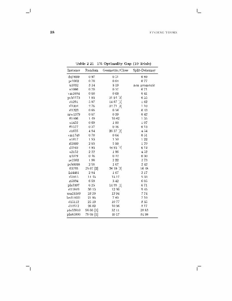
Table 2.21. 1% Optimality Gap (10 Trials)

Instance Random Geometric/Close Split-Delaunay

dsj1000 0.97 0.51 0.89pr1002 0.70 0.64 0.77si1032 3.14 3.19 non-geometricu1060 0.70 0.57 0.71vm1084 0.60 0.68 0.41pcb1173 1.03 31.04 [3] 0.55d1291 5.07 14.07 [1] 1.62rl1304 2.76 32.71 [3] 1.10rl1323 0.68 0.58 0.43nrw1379 0.67 0.39 0.42 1400 1.49 10.82 1.35u1432 0.69 1.00 1.07 1577 0.27 0.26 0.13d1655 4.84 26.37 [2] 4.54vm1748 0.70 0.64 0.51u1817 1.83 1.50 1.22rl1889 2.65 5.88 1.70d2103 4.93 48.93 [4] 6.12u2152 2.22 1.96 4.52u2319 0.46 0.42 0.30pr2392 1.90 2.22 2.73pcb3038 2.58 1.67 2.42 3795 28.67 [2] 38.10 [3] 10.48fnl4461 2.84 1.67 3.17rl5915 14.45 15.17 5.33rl5934 6.59 3.42 6.05pla7397 6.25 14.88 [1] 6.71rl11849 30.13 12.96 9.45usa13509 23.29 12.94 7.74brd14051 21.95 7.89 7.10d15112 25.19 10.77 8.35d18512 26.02 10.96 8.17pla33810 56.66 [1] 32.11 28.83pla85900 78.08 [1] 40.17 34.38

TSPLIB TESTS 39

for non-geometric instances) in the other. The table entries give the averageCPU time (using the 500 Mhz Alpha 21164a workstation) over 10 distinctruns of Chained Lin-Kernighan. For these tests we set a CPU limit of 100seconds; an entry followed by \[k]" means that k of the trials failed to producean acceptable tour in the allotted time.

As we mentioned in the previous section, a number of the smaller instancesdo not behave well with the local kicks provided by the geometric or closeprocedures. Indeed, on the instances having less than 10,000 cities, we reachedthe time limit in 17 cases when using geometric kicks, while only 2 cases failedwhen using random kicks. On the other hand, the average running time foreach of the larger instances was signi�cantly better when using geometrickicks. We therefore propose a hybrid method where we use random kickson instances having less than 10,000 cities, but we switch to geometric kickson instances having more than 10,000 cities. We report on this approach inthe third set of results in Table 2.21, using the Delaunay triangulation asour nearest-neighbor graph. (There is no entry for si1032 since this is not aEuclidean example.) We recorded no failures in this third set of tests, and,for the larger instances, the average running times were slightly better thanthe best of the 3-quad-nearest results.

In Figure 2.12, we plot the running times for the entire set of 110 TSPLIBinstances. Each of the marks in the �gure represents the mean CPU time over10 independent runs of Chained Lin-Kernighan. In these tests, we adoptedthe hybrid random/geometric approach, and used the Delaunay graph forEuclidean instances, the 3-quad-nearest graph for non-Euclidean geometricinstances, and the 12-nearest graph for non-geometric instances. The targettour was obtained in less than 0.1 seconds for all instances having at most200 cities and, with the exception of the instance a280, the target tour wasobtained in under 1.0 seconds for all instances having at most 1,000 cities.

High Quality Solutions

The above discussion points out that Chained Lin-Kernighan is a suitablemethod for obtaining reasonable quality tours in small amounts of CPU time.The real strength of the algorithm, however, is that is can e�ectively use largeramounts of CPU time to obtain much higher quality results. This feature ofChained Lin-Kernighan distinguishes it from other tour-�nding proceduresthat have been proposed thus far in the literature.

In Table 2.22, we report on 10 longer runs for the three TSPLIB instancespcb3038, usa13509, and pla85900. These examples are representative of thelarger instances in the library. We set time limits for the tests at 250 secondsfor pcb3038, 1,000 seconds for usa13509, and 5,000 seconds for pla85900.These limits correspond to roughly 100 times the CPU time that is neededto obtain 1%-quality tours for each of the instances. The average costs of thetours obtained were within 0.17% of the optimal value for pcb3038, within0.18% of the optimal value for usa13509, and within 0.30% of a known lower

40 FINDING TOURS

10 100 1000 10000 100000Number of Cities

0.0

0.1

1.0

10.0

100.0C

PU

Sec

onds

Figure 2.12. 1% of Optimality for TSPLIB

bound for pla85900. If we take the best of the 10 tours for each of the in-stances, then the costs are within 0.09% for pcb3038, 0.16% for usa13509, and0.26% for pla85900. (The degraded tour quality for pla85900 may be due, inpart, to the weakness of the lower bound.)

Table 2.22. Longer Runs (10 Trials)

Instance CPU Seconds Mean Cost Max Cost Min Cost

pcb3038 250 137932 138036 137815usa13509 1,000 20019576 20032653 20014105pla85900 5,000 142675621 142744967 142608512

To exhibit how the quality of the tour improves over time, in Figure 2.13,we plot the cost of the tour against the number of CPU seconds used byChained Lin-Kernighan, over a single run of pla85900. The curve shown inthe �gure is typical for runs on TSPLIB instances: we get sudden jumps in

TSPLIB TESTS 41

the tour quality when a kicking sequence permits a global change in the tourstructure, and these are followed by a number of smaller improvements as thekicks provide additional local optimization. At the conclusion of the 50,000second run, the tour obtained was within 0.19% of the lower bound.

0 10000 20000 30000 40000 50000CPU Seconds

142500000

142600000

142700000

142800000

142900000

143000000

Figure 2.13. Chained Lin-Kernighan for pla85900

Optimal Solutions

One of the points stressed by Lin and Kernighan [1973] is that, in manycases, their algorithm can be adopted to �nd optimal TSP solutions. Indeed,in the abstract to their classic paper, the authors write: \The procedureproduces optimum solutions for all problems tested, `classical' problems ap-pearing in the literature, as well as randomly generated test problems, up to110 cities." Their results were obtained using the \Repeated Lin-Kernighan"approach of making independent runs on a given problem instance, and select-ing the best of the tours. We have of course argued that this process is inferior

42 FINDING TOURS

to Chained Lin-Kernighan's approach of iterating the calls to lin kernighan.But if we examine the cost curve given in Figure 2.13, it is clear that withour implementation of Chained Lin-Kernighan, there comes a point where ad-ditional running time is unlikely to lead to signi�cant further improvementsin the quality of the tour produced. Johnson [1990] and Johnson and Mc-Geoch [1997] reached this same conclusion with their implementations; theyproposed to go back to making independent runs, but this time using ChainedLin-Kernighan as the core algorithm. In Table 2.22, we have seen examples ofhow this technique can lead to improved tours, and we will now discuss thisin detail.

Let us begin with the very small examples from TSPLIB. For each of the 49instances having at most 200 cities, we made 10 independent runs of ChainedLin-Kernighan, with the optimal values as the target tours and with a CPUlimit of 1 second. We performed the test three times, using di�erent selectionsfor the neighbor graph. In the �rst test, we used the Delaunay graph forEuclidean instances, the 3-quad-nearest graph for non-Euclidean geometricinstances, and the 12-nearest graph for non-geometric instances. In the secondtest, we used the 3-quad-nearest graph for all geometric instances and the 12-nearest graph for non-geometric instances. In the �nal test, we used the5-quad-nearest graph for geometric instances and the 20-nearest graph fornon-geometric instances. The number of times the codes failed to �nd optimaltours were

Delaunay 3-Quad Nearest 5-Quad Nearest

20 33 48

for the sets of 490 test runs. The failures were spread across a number ofinstances, with every example being solved at least 3 times in the Delaunayruns and at least 3 times in the 3-quad-nearest runs. In the 5-quad-nearestruns, the instance d198 was not solved in any of the 10 trials. This instancewas also the worst example in both the Delaunay and 3-quad-nearest tests,so we choose it to discuss in greater detail.

In Table 2.23, we report on a series of additional tests on d198. In theseruns, we varied the CPU limit from 0.1 seconds up to 10 seconds. For eachvalue, we made 1,000 independent trials of Chained Lin-Kernighan, recordingthe mean CPU times between occurrences of optimal solutions. These timesare reported in seconds in Table 2.23. On this instance, the Delaunay graphperformed better than the (denser) 3-quad-nearest graph. Using the Delaunaygraph, the number of times we actually found optimal solutions in the 1,000trials ranged from 13, with the 0.1 second limit, up to 967, when we allotted10 seconds for the runs. With the 3-quad-nearest, we were unable to obtainan optimal solution when we limited the runs to 0.1 seconds, but with a 10second limit we achieved the optimal value in 730 of the trials.

TSPLIB TESTS 43

Table 2.23. Optimal Solutions for d198 (1,000 Trials)

Time Limit Time per Tour (Delaunay) Time per Tour (3-Quad)

0.1 7.68 NO TOUR0.2 3.12 19.980.5 1.97 8.761.0 1.97 5.942.0 2.19 5.685.0 2.51 6.7610.0 2.64 7.19

Table 2.24. Optimal Solutions with 10 Second Limit (1,000 Trials)

Instance Time per Tour (Delaunay) Time per Tour (Quad-3)

gr202 non-Euclidean 3.69ts225 0.69 0.14tsp225 0.24 0.35pr226 0.08 0.98gr229 non-Euclidean 17.25gil262 1.37 0.80pr264 0.27 0.56a280 93.83 0.17pr299 33.84 3.46lin318 11.11 7.92rd400 42.28 75.04 417 6.69 14.00gr431 non-Euclidean 74.72pr439 6.69 4.26pcb442 7.96 6.93d493 179.23 245.68att532 non-Euclidean 95.03ali535 non-Euclidean 44.02si535 non-geometric 1427.14pa561 non-geometric 44.89u574 17.23 28.33rat575 829.64 551.97p654 13.78 21.79d657 380.73 117.37gr666 non-Euclidean 1425.67u724 318.45 412.64rat783 18.15 19.43

44 FINDING TOURS

We consider next the remaining TSPLIB instances having less than 1,000cities. These examples range in size from 202 cities up to 783 cities, includ-ing 27 instances in total. For examples in this range, it becomes di�cult toproduce optimal solutions using the straight version of Lin-Kernighan. For ex-ample, Johnson [1990] reported that a good implementation of Lin-Kernighanwas unable to �nd an optimal solution to att532 in 20,000 independent trials.Using the extra power of Chain Lin-Kernighan, however, Johnson [1990] andJohnson and McGeoch [1997] report that optimal solutions for a number ofthe examples could be found in reasonable amounts of CPU time, includingthe instances lin318, pcb442, and att532.

In our tests on these mid-sized instances, we set a 10 second time limit onthe individual calls to Chained Lin-Kernighan. We carried out 1,000 inde-pendent runs on each instance, using both the Delaunay and 3-quad-nearestgraphs. In Table 2.24, we again report the mean time between occurrences ofoptimal solutions. Although we could indeed �nd optimal solutions for each ofthe test instances, we need to point out that in a number of cases the requiredCPU times are far above those required for solving the given instances withour linear programming based branch-and-bound code.

In several of the cases requiring large amounts of computation, the problemactually lies with the choice of the neighbor graph. For these instances, tokeep the algorithm from frequently getting trapped in nonoptimal solutions,we need a broader collection of neighbors than those provided by our relativelysparse graphs. For example, with the non-geometric instance si535, if weswitch from using the 12-nearest graph to using the 40-nearest graph, thenthe average time to �nd an optimal tour drops from 1427.14 seconds down to185.81 seconds.

In other cases, such as gr666, the di�culty appears to be more fundamental.Increasing the size of the neighbor sets in gr666 does not improve the timeneeded for obtaining optimal solutions. We will come back to this example inthe next section, when we discuss a more robust procedure for using multipleruns of Chained Lin-Kernighan.

We now move on to the TSPLIB instances in the range of 1,000 cities upto 2,000 cities. In Table 2.25, we report results for this set of 17 instances,running 100 trials of Chained Lin-Kernighan with a time limit of 100 seconds.As before, we report the number of seconds between occurrences of optimaltours. Unlike the tests on small instances, however, in a number of theseruns we were not successful in producing the optimum. Indeed, we failedin 5 cases when we used the Delaunay graph and in 4 cases when we usedthe 3-quad-nearest graph. Moreover, increasing the density of the neighborsets by moving to the 10-quad-nearest graph only made matters worse|thenumber of failures went up to 6 out of the 17 instances. Nonetheless, itis interesting that such a straightforward use of Chained Lin-Kernighan canproduce optimal solutions on more than three-quarters of the instances of thissize.

TSPLIB TESTS 45

Table 2.25. Optimal Solutions with 100 Second Limit (100 Trials)

Instance Time per Tour (Delaunay) Time per Tour (3-Quad)

dsj1000 2457.30 4960.29pr1002 98.65 60.53si1032 non-geometric 26.79u1060 2457.01 2467.15vm1084 947.04 463.87pcb1173 367.34 1621.58d1291 397.37 1198.94rl1304 182.83 704.50rl1323 2453.77 4936.07nrw1379 NO TOUR 9974.98 1400 75.88 49.67u1432 1964.72 663.03 1577 NO TOUR NO TOURd1655 441.85 1077.62vm1748 9985.21 9980.64u1817 NO TOUR NO TOURrl1889 NO TOUR NO TOUR

When we proceed to even larger instances, we encounter even more failures,naturally. In Table 2.26, we report on the remaining instances having less than4,000 cities. We did not include d2103 in this set of tests, since the optimal

Table 2.26. Optimal Solutions with 250 Second Limit (100 Trials)

Instance Time per Tour (3-Quad)

u2152 24798.65u2319 NO TOURpr2392 3082.64pcb3038 NO TOUR 3795 NO TOUR

value for this instance has not (as of this writing) been determined. Using100 trials with the 3-quad-nearest graph, and with a 250 second time limit,we found optimal solutions for 2 of the 5 instances.

We remark that, using ad hoc methods, it is possible to coax Chained Lin-Kernighan into producing optimal tours for those instances in Tables 2.25 and2.26 where our multiple short runs failed. (For example, increasing the breadthparameters, using longer runs, using Martin, Otto, and Felten's simulatedannealing-like approach for accepting tours, etc.) We were not able to dothis, however, on any of the examples having greater than 4,000 cities. Foreach of these larger instances, the optimal solutions (when known) were found

46 FINDING TOURS

either by a branch-and-bound search or by the method we present in the nextsection.

2.6 TOUR MERGING

A valid criticism of the multiple-run Chained Lin-Kernighan procedure wedescribed at the end of the previous section is that in choosing only the bestof a large collection of tours, we may be discarding a great deal of valuableinformation. A challenge is to utilize the combined content of the tours toproduce a �nal tour that is superior to any single one in the collection. Thisis the same task that confronts designers of genetic algorithms for the TSP,as described, for example, in Oliver, Smith, and Holland [1987], M�uhlenbein,Gorges-Schleuter, and Kr�amer [1988], and Ulder, Aarts, Bandelt, Laarhoven,and Pesch [1991]. In our context, however, the quality of the population oftours is such that the simple randomized techniques used in successful ge-netic algorithms are very unlikely to produce tour improvements. Instead, wepropose a tour-merging procedure that attempts to produce the best possiblecombination of tours by solving a TSP restricted to the edges that are presentin at least one tour in the collection.

To illustrate our procedure, consider the 1577-city TSPLIB instance 1577.In Table 2.25 we reported that 100 trials of Chained Lin-Kernighan with atime limit of 100 seconds failed to produce the optimal 1577-tour on even asingle occasion. This instance was the smallest for which we were unable toobtain an optimal tour in our 100-trial tests. It is, however, possible to �nd anoptimal tour with the process we describe in this section. For example, making25 runs of Chained Lin-Kernighan with a 10-second time limit, we assemblethe graph represented in Figure 2.14. The edge set of this graph is the unionof the 25 edge sets of the tours; the graph has 2391 edges in total. Solvinga TSP restricted to such a sparse edge set can be much simpler than solvingthe original problem. Indeed, using our linear-programming-based TSP code(see Applegate, Bixby, Chv�atal, and Cook [1998]), the optimal solution to therestricted problem was found in 469.8 seconds on a 500 Mhz Alpha 21164aprocessor workstation. In this example, moreover, the tour produced is alsooptimal for the original TSP instance. The total time to obtain this optimalsolution was approximately 12 minutes.

Tour-merging is a powerful method for obtaining tours of quality exceedingthat of the standard multiple-run Chained Lin-Kernighan procedure. It is notonly an e�ective way of expending large amounts of computational resourcesto obtain the best quality tours, but also a very competitive procedure formodest length computational runs on a wide range of problem instances. Aswe shall describe, however, care needs to be taken so that the solve times ofthe sparse TSPs do not become unacceptably long.

We begin our discussion with the collection of TSPLIB instances having lessthan 1,000 cities. From this set, all instances having less than 200 cities are

TOUR MERGING 47

Figure 2.14. Union of 25 Chained Lin-Kernighan Tours for 1577

48 FINDING TOURS

solved handily with Chained Lin-Kernighan, so we will not consider furtherthese instances. In Table 2.24, we reported results for the remaining examplesusing multiple 10-second runs of Chained Lin-Kernighan. Of the 27 instancesconsidered in Table 2.24, only 5 required an average time of greater than 2minutes to �nd optimal solutions. The average times for these 5 most di�cultinstances ranged from 245 seconds for d493 to 1,427 seconds for si535. Wewill use these 5 examples as our initial testbed for tour merging.

For each of the 5 instances, we made 10 trials of merging 25 tours found withChained Lin-Kernighan, giving each Chained Lin-Kernighan run a 2.5 secondtime limit. In these tests, we used the 3-quad-nearest graph to determine theneighbor sets for Chained Lin-Kernighan, and we used the nearest-neighboralgorithm to produce the starting tours. The results are reported in Table 2.27(again using a 500 Mhz Alpha 21164a workstation). The column labeled \LK-

Table 2.27. Tour Merging with 25 Tours and 2.5 Second Limit (10 Trials)

Instance LK-quality Merge-quality LK-opt Merge-opt Time (seconds)

d493 1.00039 1.00000 0 10 167.76si535 1.00120 1.00007 0 5 85.02rat575 1.00025 1.00009 1 4 125.38gr666 1.00061 1.00006 0 8 97.90u724 1.00044 1.00000 0 10 135.37

quality" gives the average ratio of the cost of the best of the 25 ChainedLin-Kernighan tours in each trial, to the cost of an optimal tour; the columnlabeled \Merge-quality" gives the average ratio of the cost of the �nal mergedtour for each trial, to the cost of an optimal tour; \LK-opt" reports the numberof trials for which the best Chained Lin-Kernighan tour was optimal, and\Merge-opt" reports the number of times the �nal merged tour was optimal.

In 37 of the 50 trials the merged tour was indeed optimal, and the averagetour quality over all trials was 1.00004, that is, on average the tours producedwere within 0.004% of the optimal values. To compare these results withthose given in Table 2.24, note that the average time between appearances ofoptimal solutions ranged from 135 seconds for u724 to 313 seconds for rat575.

In the above tests, the sparse TSP instances were solved in an average timeof under 50 seconds with the linear-programming-based code. Although thesesolve times are quite acceptable, in many cases alternative methods can treatthe sparse problems more e�ectively than the general purpose code of Apple-gate, Bixby, Chv�atal, and Cook [1998]. One attractive alternative is to usethe branch-width graph invariant proposed by Robertson and Seymour [1991]to solve the sparse TSPs via dynamic programming. This idea is treated inCook and Seymour [1999].

The combination of N = 25 tours and a time limit of T = 2:5 seconds onChained Lin-Kernighan gives a reasonable compromise between tour quality

TOUR MERGING 49

and total running time for the under 1000-city examples. In Table 2.28 wecompare these results (over the 50 total trials), with the results for severalother combinations of N and T . Note that the average running time for

Table 2.28. Tour merging with 5 instances having less than 1000 cities

Number of Tours Time Limit (seconds) Tour Quality Time (seconds)

5 5 1.00042 39.2410 2.5 1.00045 54.9210 5 1.00014 74.3625 1 1.00017 137.0425 2.5 1.00004 122.2925 5 1.00003 170.20

N = 25 and T = 1 is higher than the time for N = 25 and T = 2:5, despitethe much lower time for computing the collection of tours. The explanation isthat the lower quality Chained Lin-Kernighan tours lead to a lessor number ofrepeated edges in the tour population, and therefore a denser (more di�cult)TSP instance to be solved.

Let us now consider the TSPLIB instances in the range of 1,000 cities up to2,000 cities. The results for multiple 100-second Chained Lin-Kernighan runsfor this class of 17 examples is presented in Table 2.25. The three instances 1577, u1817, and rl1889 were not solved in the 100 trials considered in thosetests, while the average running times for the remaining instances varied from27 seconds up to 9980 seconds (to obtain optimal solutions). In our tour-merging tests, we will treat the 13 instances that required greater than 600seconds, including the 3 examples that were not solved. The results for thisproblem set, using N = 25 and T = 10, are given in Table 2.29. Withthese settings, optimal solutions were found in 95 of the 130 trials, and everyinstance was solved at least 2 times. The running times are modest, withthe exception of u1817, which required an average of nearly 11,000 seconds tosolve the sparse TSPs. A direct precaution against such behavior is to set anupper bound on the time allowed in the TSP solver, reporting a failure if thebound is reached. For example, setting a bound of 5,000 seconds lowers theaverage running time to 4451.83 seconds for u1817, while still reaching theoptimal solution on 5 of the 10 trials.

In Table 2.30 we compare several di�erent choices of N and T for the setof 13 instances considered in Table 2.29. The values reported are the averagesover all 130 trials. The quality of the �nal tour drops quickly as we decreasethe size of the tour population, but there is a corresponding decrease in thetime required to solve the resulting sparse TSP instances.

Proceeding to larger examples, let us again consider the 5 TSPLIB instancesunder 4,000 cities that we treated in Table 2.26. These are all TSPLIB in-stances in the range of 2,000 to 4,000 cities, with the exception of d2103 (the

50 FINDING TOURS

Table 2.29. Tour Merging with 25 Tours and 10 Second Limit (10 Trials)

Instance LK-quality Merge-quality LK-opt Merge-opt Time (seconds)

dsj1000 1.00094 1.00032 0 4 356.14u1060 1.00070 1.00000 0 10 519.00pcb1173 1.00013 1.00000 4 8 385.89d1291 1.00091 1.00000 0 10 415.38rl1304 1.00143 1.00038 0 7 263.78rl1323 1.00114 1.00011 0 6 324.58nrw1379 1.00046 1.00000 0 8 458.37u1432 1.00099 1.00000 0 10 1337.15 1577 1.00123 1.00021 0 2 633.36d1655 1.00102 1.00002 0 8 450.12vm1748 1.00057 1.00000 0 10 347.71u1817 1.00253 1.00017 0 7 11231.06rl1889 1.00214 1.00002 0 5 451.42

Table 2.30. Tour merging with 13 instances having between than 1000

and 2000 cities

Number of Tours Time Limit (seconds) Tour Quality Time (seconds)

5 50 1.00098 339.4410 10 1.00045 422.2510 25 1.00045 476.2225 10 1.00009 1321.07

TOUR MERGING 51

optimal value for d2103 has not yet been determined). In the tests reported inTable 2.26, optimal solutions were found only for instances u2152 and pr2392,requiring an average of 24,799 seconds and 3,083 seconds, respectively. InTable 2.31, we report tour-merging results for 10 trials on each of the 5 testinstances, using N = 25 and T = 10. Optimal solutions were obtained in 41 of

Table 2.31. Tour Merging with 25 Tours and 10 Second Limit (10 Trials)

Instance LK-quality Merge-quality LK-opt Merge-opt Time (seconds)

u2152 1.00199 1.00000 0 10 6026.40u2319 1.00172 1.00000 0 10 28097.92pr2392 1.00124 1.00000 0 10 303.68pcb3038 1.00190 1.00001 0 8 16196.12 3795 1.00592 1.00031 0 3 4808.10

the 50 trials, and each example was solved at least 3 times. This is certainly animprovement over our multiple Chained Lin-Kernighan runs, but the runningtimes for two of the instances, u2319 and pcb3038, exceeded 10,000 seconds.The u2319 example can be solved easily using other methods (for example,the branch-width technique we mentioned brie y above), so we select pcb3038for further discussion.

In Table 2.32 we report results of 10 trials on pcb3038 using a variety ofsettings for N and T . These results illustrate several common properties of

Table 2.32. Tour Merging on pcb3038 (10 Trials)

Settings LK-quality Merge-quality Merge-opt Time (seconds)

N = 25; T = 10 1.00190 1.00001 8 16196.12N = 25; T = 50 1.00103 1.00001 7 10042.43N = 25; T = 100 1.00096 1.00002 5 7006.48N = 25; T = 250 1.00071 1.00000 10 11318.06N = 25; T = 500 1.00063 1.00002 7 16145.61N = 25; T = 1000 1.00059 1.00000 9 28781.31

N = 10; T = 100 1.00145 1.00024 0 3631.65N = 10; T = 250 1.00090 1.00009 1 4029.43N = 10; T = 500 1.00095 1.00008 3 6526.59N = 10; T = 1000 1.00059 1.00008 3 10963.02

tour-merging runs. Firstly, the quality of the �nal tour depends heavily on thesize of the population of tours, but only to a lessor degree on the time limitgiven to Chained Lin-Kernighan (as long as the limit is reasonably large).Secondly, the solution time for the sparse TSP decreases dramatically as thequality of the tours in the population is improved, that is, for �xed N , the

52 FINDING TOURS

sparse TSP time decreases as T is increased. To select the best settings ofN and T , we must trade o� the time used to produce the tour populationversus the time needed to solve the sparse TSPs. This is a di�cult task onlarge instances, since the performance of the linear-programming-based codeis di�cult to predict without running experiments.

To apply tour merging to even larger instances, we need to take great carein the selection of the tour population. For example, 10 trials on the instancefnl4461 produced the following results

LK-quality Merge-quality LK-opt Merge-opt Time

1.00078 1.00000 0 10 85920.98

using N = 25 and T = 100. The fact that the optimal tour was obtainedin each of the trials is a very positive sign, but the average running time forthe sparse TSPs is very high (the full instance was solved in less than 150,000seconds by Applegate, Bixby, Chv�atal, and Cook [1998]). It possible, however,to use Chained Lin-Kernighan to obtain tour populations that are much morelikely to be amenable to sparse TSP solution routines. What is needed ismore homogeneous collection of tours. To achieve this, rather than using thenearest-neighbor algorithm to produce di�erent starting tours for each run,we can start the Chained Lin-Kernighan runs from a common starting tourthat is itself the result of a run of Chained Lin-Kernighan. This adds a thirdsetting for our runs, namely the number of seconds S used in the initial runto build the common starting tour.

In Table 2.33 we report results for fnl4461, where we �x N and T , andpermit S to vary between 5, 10, and 25. As one would expect, as we increase

Table 2.33. Tour Merging on fnl4461 with Fixed Start (10 Trials)

Settings LK-quality Merge-quality Time (seconds)

N = 25; T = 100; S = 5 1.00099 1.00065 3911.41N = 25; T = 100; S = 10 1.00106 1.00074 2828.08N = 25; T = 100; S = 25 1.00111 1.00087 2690.53

N = 25; T = 50; S = 5 1.00128 1.00076 3875.04N = 25; T = 50; S = 10 1.00121 1.00082 1681.37N = 25; T = 50; S = 25 1.00123 1.00092 1352.63

the quality of the common starting tour, the time needed to solve the sparseTSP drops, but at the expense of lowering the average quality of the �nalmerged tour.

The added exibility of using a high quality common starting allows us toapply tour-merging to a very wide range of instances. To illustrate this, we

TSPLIB TOURS 53

consider pla85000, the largest instance in the TSPLIB. On an instance of thissize, there is a large variance in the quality of tours produced by individualruns of Chained Lin-Kernighan, so before we invest the time to obtain anentire collection of tours, it is important to make an e�ort to have a commonstarting tour that is likely to lead to a high quality population. To achievethis, we can use a short multiple Chained Lin-Kernighan run to obtain thecommon tour, rather than simply using a single run. In our case, making 5runs of Chained Lin-Kernighan, with a time limit of 1,000 seconds, we obtaintours of the following costs

142880000; 142744923; 142732749; 142754147; 142866379:

Now, making 5 further Chained Lin-Kernighan runs using the best of these(142732749) as a starting tour, and using a 5,000 second time limit, we obtainthe population

142628651; 142603285; 142613880; 142625393; 142624904:

With this collection, the merged tour can be computed in 153,034 additionalseconds, resulting in a tour of cost 142575637. The TSP solve time is ex-tremely high due to the fact that 85,900 cities is well beyond the size ofinstances targeted by the Applegate, Bixby, Chv�atal, and Cook [1998] code,but this example does indicate that tour-merging is a viable approach, evenfor instances of this size.

Tour-merging can be used in a wide variety of ways, and it is likely thatideas drawn from the �eld of genetic algorithms can be combined with tourmerging to produce a powerful class of heuristics. On large examples, our useof the procedure has been con�ned primarily to ad hoc methods, but, as wereport in the next section, we have nonetheless been able to obtain the bestcurrently known results for each of the unsolved TSPLIB instances. It wouldcertainly appear that tour merging is an area that holds promise for furtherimprovement in tour �nding algorithms.

2.7 TSPLIB TOURS

In Table 2.34, we report the costs of the cheapest tours we have found, withour heuristic methods, for the instances in TSPLIB that were unsolved as of1994. The tours for four of the instances have been shown to be optimal, andthe tour for usa13509, although not optimal, is only 0.0002% more costly thanthe optimal tour. In each of the other cases, the tours give the best valuesthat have been reported to G. Reinelt [1999].

In each instance, the tour was obtained by using Chained Lin-Kernighanto produce a collection of tours, using tour merging to re�ne the collection,and repeating the process.

54 FINDING TOURS

Table 2.34. Unsolved TSPLIB Problems

Name Size Tour Cost Lower Bound Gap

1577 1,577 22249 22249 OPTIMALd2103 2,103 80450 80330 0.15% 3795 3,795 28772 28772 OPTIMALrl5915 5,915 565530 565530 OPTIMALrl5934 5,934 556045 556045 OPTIMALrl11849 11,849 923368 923132 0.03%usa13509 13,509 19982889 19982859 0.00%brd14051 14,051 469445 469272 0.04%d15112 15,112 1573152 1572863 0.02%d18512 18,512 645300 645198 0.02%pla33810 33,810 66116530 65970716 0.22%pla85900 85,900 142473573 142253424 0.16%

The lower bounds were computed using our linear-programming-based codefor the TSP, as described in Applegate, Bixby, Chv�atal, and Cook [1998].Again, in each case the lower bounds are the best bounds that have beenreported to G. Reinelt [1999].

B i b l i o g r a p h y

D. Applegate, V. Chv�atal, and W. Cook (1990). \Lower bounds for the trav-elling salesman problem", in: \TSP '90", CRPC Technical Report CRPC-TR90547, Center for Research in Parallel Computing, Rice University.

D. Applegate, R. Bixby, V. Chv�atal, and W. Cook (1998), \On the solu-tion of traveling salesman problems", Documenta Mathematica Journal

der Deutschen Mathematiker-Vereinigung, International Congress of Math-

ematicians, 645{656.

D. Applegate, W. Cook, and A. Rohe (1999). \Chained Lin-Kernighan forlarge traveling salesman problems", in preparation.

F. Aurenhammer (1991). \Voronoi diagrams: a survey of a fundamental datastructure", ACM Computational Surveys 23, 345{405

A. Bachem and M. Wottawa (1992). \Parallelisierung von heuristiken f�urgrosse traveling-salesman-probleme", Report Number 92.119, Mathematis-ches Institut, Universit�at zu K�oln.

J. J. Bartholdi III and L. K. Platzman (1982). \An O(NlogN) planar travel-ling salesman heuristic based on space�lling curves", Operations ResearchLetters 1, 121{125.

J. L. Bentley (1990). \Experiments on traveling salesman heuristics", in: FirstAnnual ACM-SIAM Symposium on Discrete Algorithms, San Francisco, pp.91{99.

J. L. Bentley (1992). \Fast algorithms for geometric traveling salesman prob-lems", ORSA Journal on Computing 4, 387{411.

R. G. Bland and D. F. Shallcross (1989). \Large traveling salesman problemsarising from experiments in X-ray crystallography: a preliminary report oncomputation", Operations Research Letters 8, 125{128.

F. Bock (1958). Research Report, Armour Research Foundation. (Presented atthe Operations Research Society of America Fourteenth National Meeting,St. Louis, October 24, 1958.)

O. Bor�uvka (1926). \On a certain minimal problem" (in Czech), Pr�ace

Moravsk�e P�r��rodov�edeck�e Spole�cnosti 3, 37{58.

55

56 BIBLIOGRAPHY

N. Christo�des (1976). \Worst-case analysis of a new heuristic for the travel-ling salesman problem", Report Number 388, Graduate School of IndustrialAdministration, Carnegie Mellon University.

M. Chrobak, T. Szymacha, and A. Krawczyk (1990). \A data structure usefulfor �nding Hamiltonian cycles", Theoretical Computer Science 71, 419{424.

B. Codenotti, G. Manzini, L. Margara, and G. Resta (1996). \Perturbation:an e�cient technique for the solution of very large instances of the EuclideanTSP", INFORMS Journal on Computing 8, 125{133.

W. Cook and P. D. Seymour (1999). \A branch-decomposition heuristic forthe TSP", in preparation.

G. A. Croes (1958). \A method for solving traveling-salesman problems",Operations Research 5, 791{812.

H. Edelsbrunner (1987). Algorithms in Combinatorial Geometry, Springer,Heidelberg.

M. M. Flood (1956). \The traveling-salesman problem", Operations Research4, 61{75.

S. J. Fortune (1987). \A sweepline algorithm for Voronoi diagrams", Algo-rithmica, 153{174.

S. J. Fortune (1994). \sweep2", computer code available via anonymous ftpfrom netlib.att.com.

M. L. Fredman, D. S. Johnson, L. A. McGeoch, and G. Ostheimer (1995).\Data structures for traveling salesmen", Journal of Algorithms 18, 432{479.

M. Gr�otschel and O. Holland (1991). \Solution of large-scale symmetric trav-elling salesman problems", Mathematical Programming 51, 141{202.

I. Hong, A. B. Kahng, and B. Moon (1998). \Improved large-step markovchain variants for the symmetric TSP", to appear in Journal of Heuristics.

B. W. Kernighan and D. M. Ritchie (1978). The C Programming Language,Prentice Hall, Englewood Cli�s.

D. S. Johnson (1990). \Local optimization and the traveling salesman prob-lem", in: Proceedings 17th Colloquium of Automata, Languages, and Pro-

gramming, Lecture Notes in Computer Science, Volume 443, Springer-Verlag, Berlin, pp. 446{461.

D. S. Johnson, J. L. Bentley, L. A. McGeoch, and E. E. Rothberg (1999). Inpreparation.

D. S. Johnson and L. A. McGeoch (1997). \The traveling salesman problem:a case study in local optimization", in: Local Search in Combinatorial Op-

timization (E. H. L. Aarts and J. K. Lenstra, eds.), Wiley, New York, pp.215{310.

BIBLIOGRAPHY 57

M. J�unger, G. Reinelt, and G. Rinaldi (1995). \The traveling salesman prob-lem", in: Handbook on Operations Research and Management Sciences:

Networks (M. Ball, T. Magnanti, C. L. Monma, and G. Nemhauser, eds.),North-Holland, pp. 225{330.

D. E. Knuth (1973). Sorting and Searching, The Art of Computer Program-

ming, Volume 3, Addison Wesley, Reading.

E. L. Lawler, J. K. Lenstra, A. H. G. Rinnooy Kan, and D. B. Shmoys, eds.(1985). The Traveling Salesman Problem, Wiley, Chichester.

S. Lin (1965). \Computer solutions of the traveling salesman problem", TheBell System Technical Journal 44, 2245{2269.

S. Lin and B. W. Kernighan (1973). \An e�ective heuristic algorithm for thetraveling-salesman problem", Operations Research 21, 498{516.

K.-T. Mak and A. J. Morton (1993). \A modi�ed Lin-Kernighan traveling-salesman heuristic", Operations Research Letters 13, 127{132.

F. Margot (1992). \Quick updates for p-opt TSP heuristics", Operations Re-search Letters 11, 45{46.

O. Martin, S. W. Otto, and E. W. Felten (1991). \Large-step Markov chainsfor the traveling salesman problem", Complex Systems 5, 299{326.

O. Martin, S. W. Otto, and E. W. Felten (1992). \Large-step Markov chainsfor the TSP incorporating local search heuristics", Operations Research

Letters 11, 219{224.

O. C. Martin and S. W. Otto (1996). \Combining simulated annealing withlocal search heuristics", Annals of Operations Research 63, 57{75.

K. Mehlhorn (1984). Multi-dimensional Searching and Computational Geom-

etry, Springer, Berlin.

G. Morton and A. H. Land (1955). \A contribution to the `travelling-salesman'problem", Journal of the Royal Statistical Society, Series B, 17, 185{194.

H. M�uhlenbein, M. Gorges-Schleuter, and O. Kr�amer (1988). \Evolution al-gorithms in combinatorial optimization", Parallel Computing 7, 65{85.

D. M. Neto (1999), E�cient Cluster Compensation for Lin-Kernighan Heuris-

tics, Ph.D. Thesis, Department of Computer Science, University of Toronto.

I. M. Oliver, D. J. Smith, and J. R. C. Holland (1987). \A study of permuta-tion crossover operators on the traveling salesman problem", J.J. Grefen-stette (ed.), Genetic Algorithms and Their Applications: Proceedings of

the Second International Conference on Genetic Algorithms, Lawrence Erl-baum Associates, Hillsdale, New Jersey, pp. 224{230.

M. Padberg and G. Rinaldi (1991). \A branch-and-cut algorithm for the reso-lution of large-scale symmetric traveling salesman problems", SIAM Review

33, 60{100.

58 BIBLIOGRAPHY

J. Perttunen (1994). \On the signi�cance of the initial solution in travellingsalesman heuristics", Journal of the Operational Research Society 45, 1131{1140.

G. Reinelt (1991). \TSPLIB - A traveling salesman library", ORSA Journal

on Computing 3, 376{384.

G. Reinelt (1991a). \TSPLIB - Version 1.2", Report Number 330, Schwer-punktprogramm der Deutschen Forschungsgemeinschaft, Universit�at Augs-burg.

G. Reinelt (1992). \Fast heuristics for large geometric traveling salesman prob-lems", ORSA Journal on Computing 4, 206{217.

G. Reinelt (1994). The Traveling Salesman: Computational Solutions for TSPApplications, Springer-Verlag, Berlin.

G. Reinelt (1995). \TSPLIB95", Interdisziplin�ares Zentrum f�ur Wis-senschaftliches Rechnen (IWR), Heidelberg. (Manuscript and problem in-stances available via anonymous ftp:ftp://ftp.iwr.uni-heidelberg.de/pub/tsplib.)

G. Reinelt (1999). Personal communication.

S. Reiter and G. Sherman (1965). \Discrete optimizing", SIAM Journal on

Applied Mathematics 13, 864{889.

N. Robertson and P. D. Seymour (1991). \Graph minors. X. Obstructionsto tree-decomposition", Journal of Combinatorial Theory, Series B, 52,153{190.

A Rohe (1997). Parallele Heuristiken f�ur sehr grosse Traveling Salesman Prob-leme, Diplomarbeit, Research Institute for Discrete Mathematics, Univer-sit�at Bonn.

M. Sch�afer (1994). E�ziente Algorithmen f�ur sehr grosse Traveling Salesman

Probleme, Diplomarbeit, Research Institute for Discrete Mathematics, Uni-versit�at Bonn.

D. Shallcross (1990). Personal communication.

D. D. Sleator and R. E. Tarjan (1983). \Self-adjusting binary trees", Proceed-ings of the Fifteenth Annual SCM Symposium on Theory of Computing,ACM, pp. 235{245.

R. E. Tarjan (1983). Data Structures and Network Algorithms, SIAM,Philadelphia.

N. L. J. Ulder, E. H. L. Aarts, H.-J. Bandelt, P. J. M. Laarhoven, and E.Pesch (1991). \Genetic local search algorithms for the traveling salesmanproblem", in: Parallel Problem Solving from Nature (H.-P. Schwefel and R.M�anner, eds.), Elsevier Science Publishers, Amsterdam, pp. 65{74.

M. G. A. Verhoeven, P. C. J. Swinkels, and E. H. L. Aarts (1995). \Parallellocal search for the traveling salesman", Working Paper, Philips ResearchLaboratories, Eindhoven.

BIBLIOGRAPHY 59

M. G. A. Verhoeven, E. H. L. Aarts, E. van de Sluis, and R. J. M. Vassens(1995). \Parallel local search and the travelling salesman problem", in:Parallel Problem Solving from Nature 2 (R. M�anner and B. Manderick,eds.), North-Holland, Amsterdam, pp. 543{552.