Finding the Homology of Submanifoldswith High Confidence from Random

Samples∗

P. Niyogi†, S. Smale‡, S. Weinberger§

March 15, 2006

Abstract

Recently there has been a lot of interest in geometrically moti-vated approaches to data analysis in high dimensional spaces. Weconsider the case where data is drawn from sampling a probabilitydistribution that has support on or near a submanifold of Euclideanspace. We show how to “learn” the homology of the submanifoldwith high confidence. We discuss an algorithm to do this and pro-vide learning-theoretic complexity bounds. Our bounds are obtainedin terms of a condition number that limits the curvature and nearnessto self-intersection of the submanifold. We are also able to treat thesituation where the data is “noisy” and lies near rather than on thesubmanifold in question.

∗The main results of this paper were first presented at a conference in honor of JohnFranks and Clark Robinson at Northwestern University in April 2003. These results wereformally written as Technical Report No. TR-2004-08, Department of Computer Science,University of Chicago.

†Departments of Computer Science, Statistics, University of Chicago.‡Toyota Technological Institute, Chicago.§Department of Mathematics, University of Chicago.

1

1 Introduction

In recent years, there has been considerable interest in the possibility ofanalyzing and processing data in high dimensional spaces. Following theintuition that naturally occurring data may be generated by structuredsystems with possibly much fewer degrees of freedom than the ambientdimension would suggest, various researchers (see [11, 8, 9, 12, 7] haveconsidered the case when the data lives on or close to a submanifold ofthe ambient space. One hopes then to estimate geometrical and topolog-ical properties of the submanifold from random points (“scattered data”)lying on this unknown submanifold. These questions belong to a class ofproblems that have come to be known as manifold learning.In this paper, we consider the particular question of identifying the homol-ogy of the submanifold from random samples. The homology of the sub-manifold (see [15] for definitions) are natural topological invariants thatprovide a good characterization of many aspects of it. For example, thedimensions of the homology groups, the Betti numbers (b0, b1 . . .) have nat-ural interpretations. b0, the dimension of the zeroth homology group is thenumber of connected components of the submanifold. In data analysis sit-uations, the number of clusters of the data may sometimes be understoodin terms of the number of components of an underlying manifold (or othergeometric object). If the dimension of the submanifold is d, then one seesthat bj = 0 for all j > d. Thus the the largest non-trivial homology gives usthe dimension of the submanifold. If the submanifold is two-dimensional,then b0 and b1, are related to the number of connected components andnumber of holes respectively of the submanifold.We show that it is possible to identify the homology from random samplesand discuss an algorithm to do this. There are a few aspects of the develop-ments in this paper that are worth emphasizing. First, we provide samplecomplexity estimates on the number of examples that are needed to iden-tify the homology with high confidence. Our results are in the style oflearning theoretic treatments (for example, the Probably Approximately Cor-rect framework [20]) where unknown objects (typically functions in learn-ing theory) are “learned” from random samples and confidence estimatesare provided. Second, we treat the situation where data might be drawnfrom a distribution that is concentrated around the manifold rather thanprecisely on it. Under specific models of noise, we show that our algo-rithm can work even with noisy data. In all cases, estimates are provided

2

in terms of a condition number that limits the curvature and nearness toself-intersection of the submanifold.Our results may also be of interest to researchers in computational ge-ometry and topology who have considered the question of computinghomology from simplicial complexes in the past (see [19, 13] for detailsand further references). A number of researchers in these computationalgeometry and topology have considered the problem of manifold recon-struction from point cloud data. Such work has typically focused on thecase of surfaces in IR3 and examples include algorithms associated withthe frameworks of alpha shapes [5], CRUST [1] and its variants, and CO-CONE [2] and its generalizations. CRUST and COCONE provably recovera simplicial 2-manifold that is homeomorphic to the surface. In [3] (writ-ten after the results of our current paper were declared), it was shown howto extend these ideas to the general setting of a k-manifold embedded inIRN . In much of this work, the medial axis plays a central role in charac-terizing the conditioning of the manifold (see our later remarks in Section2). It is also worth noting that none of the work mentioned above consid-ers the probabilistic setting where examples are drawn at random — sono high confidence guarantees are provided. The theorems in [1, 2, 3] areanalogous to our Proposition 3.1. No version of our main theorem (The-orem 3.1) exists in the literature. Finally, it is also worth noting that thereis a body of work on persistence homology [7, 6] that seeks alternativetopological characterizations of the manifold and its homology. See thediscussion after Proposition 3.1.In conclusion, we hope that researchers in graphics, pattern recognition,solid modeling, molecular biology, finance, and other areas where largeamounts of high dimensional data are available may find some use for thetopological perspective on data analysis embodied in the algorithms andanalyses of this paper.

2 Preliminaries

Consider a compact Riemannian submanifold M of a Euclidean spaceIRN . Sample the manifold according to a uniform probability measureon it. Thus points x1, . . . , xn ∈ M are generated. This set of points x ={x1, . . . , xn} will be the data set on the basis of which homology groupswill be calculated. In later sections, we will consider the case when the

3

data is drawn from a probability measure with support close to the mani-fold.Throughout our discussion, we will associate to M a condition number(1/τ ) where τ defined as the largest number having the property: The opennormal bundle about M of radius r is imbedded in IRN for every r < τ . Itsimage Tubτ is a tubular neighborhood of M with its canonical projectionmap

π0 : Tubτ → MNote that τ encodes both local curvature considerations as well as globalones: If M is a union of several components τ bounds their separation.For example, if M is a sphere, then τ is equal to its radius. If M is anannulus, then τ is the separation of its components. In Section 6 we re-late the condition number 1

τto classical notions of curvature in differential

geometry via the second fundamental form.Finally, it is also useful to relate τ to the notions of medial axis and lo-cal feature size that have been developed in the computational geometrycommunity. Given M, one may define the set

G = {x ∈ IRN such that ∃ distinct p, q ∈ M where d(x,M) = ||x−p|| = ||x−q||}

where d(x,M) = infy∈M ||x − y|| is the distance of x to M. The closure ofG is called the medial axis and for any point p ∈ M the local feature sizeσ(p) is the distance of p to the medial axis. Then it is easy to check that

τ = infp∈M

σ(p)

3 An Outline of our Main Results

Ultimately we wish to compute the homology of the manifold M ⊂ IRN

from the randomly sampled datapoints x = {x1, . . . , xn} ⊂ M. We firstbegin by considering Euclidean balls (in the ambient space IRN ) of radiusε and centers xi’s. Let us denote these balls as Bε(xi). We can now definethe open set U ⊂ IRN given by

U = ∪x∈xBε(x)

Our first proposition states that if x = {x1, . . . , xn} is ε/2 dense in M, thenM is a deformation retract of U .

4

Proposition 3.1 Let x be any finite collection of points x1, . . . , xn ∈ IRN suchthat it is ε

2dense in M, i.e., for every p ∈ M, there exists an x ∈ x such that

‖ p − x ‖IRN < ε2. Then for any ε <

√

35τ , we have that U deformation retracts to

M. Therefore homology of U equals homology of M.

We prove this proposition in Section 4. Subsequent to our work, the au-thors of [6] presented a different type of calculation of the homology ofM based on their homology approximation theorem together with themethod of computing persistent homology (e.g. [7]). Their method doesnot give the homotopy type of M. On the other hand, it does apply to aclass of metric spaces more general than well conditioned manifolds.In the case under consideration here, the points x1, . . . , xn are sampled ini.i.d. fashion from the uniform probability distribution on M. By proba-bilistic considerations, we will then prove (in Section 5)

Proposition 3.2 Let x be drawn by sampling M in i.i.d. fashion according tothe uniform probability measure on M. Then with probability greater than 1− δ,we have that x is ε

2-dense (ε < τ

2) in M provided

|x| > β1(log(β2) + log(1

δ))

where β1 = vol(M)

(cosk(θ1))vol(Bkε/4

)and β2 = vol(M)

(cosk(θ2))vol(Bkε/8

). Here k is the dimension of

the manifold M and vol(Bkε ) denotes the k-dimensional volume of the standard

k-dimensional ball of radius ε. Finally θ1 = arcsin( ε8τ

) and θ2 = arcsin( ε16τ

).

Putting these two propositions together, we see that we are able to providea finite sample estimate for how many times we need to sample M so thatwe are guaranteed with high confidence that the homology of the randomset U equals the homology of M. Thus our main theorem is

Theorem 3.1 Let M be a compact submanifold of IRN with condition number τ .Let x = {x1, . . . , xn} be a set of n points drawn in i.i.d fashion according to theuniform probability measure on M. Let 0 < ε < τ

2. Let U = ∪x∈xBε(x) be a

correspondingly random open subset of IRN . Then for all

n > β1(log(β2) + log(1

δ))

the homology of U equals the homology of M with high confidence (probability> 1 − δ).

5

Remark. Note that no version of our main theorem exists in the literatureso far. However, versions of our Proposition 3.1 do exist. We have char-acterized Proposition 3.1 in terms of τ but one may obtain an alternatecharacterization in terms of the medial axis and the local feature size. Infact, if one considers the union of balls centered at the data points givenby U = ∪x∈xBεx(x) where εx = rσ(x), then it is possible to show that thehomology of U coincides with that of M if x is εx

2-dense in M and for all

r < 0.21. For the case of surfaces in IR3, a similar result is obtained byAmenta et al for r < 0.06. The set x is said to be εx

2-dense if for every

p ∈ M there exists some x ∈ x such that ||p − x|| < εx

2. We will prove this

in a later paper. It is not obvious, however, how to obtain a version of ourmain theorem in terms of the local feature size. Finally, we recall the recentresults of [6] that we have already alluded to.

3.1 Computing the Homology of U

One now needs to consider algorithms to compute the homology of U .Noting that the Bε(xi)’s form a cover of U , one can construct the nerve ofthe cover. The nerve is an abstract simplicial complex constructed as fol-lows: One puts in a k-simplex for every k+1-tuple of intersecting elementsof the cover. The Nerve Lemma (see [10]) applies in our case, as balls areconvex, to show that the homology of U is the same as the homology ofthis complex. The algorithm consists of the following components.

1. Given an ε, and a set of points x = {x1, . . . , xn} in IRN , each j-simplexis given by a subset of the n points that have non-zero intersection.Thus we may define Lj to be the collection of all j-simplices. Eachsimplex σ ∈ Lj is associated with a set of j+1 points (p0(σ), . . . , pj(σ) ∈x) such that

∩ji=0Bε(pi(σ)) 6= ∅

An orientation for the simplex is chosen by picking an ordering andlet us denote the oriented simplex by |p0(σ), . . . , pj(σ)|.

2. A very crude upper bound on the size of Lj (denoted by |Lj|) is givenby

(

nj+1

)

. However, it is clear that if two points xm and xl are morethan 2ε apart, they cannot be associated to a simplex. Therefore, thereis a locality condition that the pi(σ)’s must obey which results in |Lj|being much smaller than this crude number. The simplicial complex

6

Kj = ∪ji=0Lj together with face relations. The simplicial complex

corresponding to the nerve of U is K = KN .

3. A basic subroutine for computing the simplicial complex (steps 1 and2 above) involves the decision problem: for any set of j points, de-termine whether balls of radius ε around each of these points havenon-empty intersection. This problem is related to the smallest ballproblem defined as follows: Given a set of j points, find the the ballwith smallest radius enclosing all these points. One can check that∩j

i=1Bε(pi) 6= ∅ if and only if this smallest radius < ε. Fast algorithmsfor the smallest ball problem exist. See [17] for theoretical discussionand “http://www2.inf.ethz.ch/personal/gaertner/miniball.html” fordownloadable algorithms from the web.

4. We will work in the field of coefficients IR. Then a j-chain is a func-tion c : Lj → IR and can be written as a formal sum

c =∑

σ∈Lj

c(σ)σ

By adding j-chains component wise, one gets the vector space of j-chains denoted by Cj .

5. The boundary operator ∂j is a linear operator from Cj to Cj−1 definedas follows. For each (oriented) simplex σ ∈ Lj ,

∂jσ =

j∑

i=0

(−1)iσi

where σi is a j − 1 face of σ (facing point pi(σ)) and the orientation ofσi is given by |p0, . . . , pi−1, pi+1, . . . , pj|. Now ∂j is defined on j chainsby additivity as

∂j(∑

σ∈Lj

c(σ)σ) =∑

σ∈Lj

c(σ)∂jσ

Thus, ∂j can be represented as a nj−1 ×nj matrix where nj−1 = |Lj−1|and nj = |Lj| respectively. The matrix is usually sparse in our setting.

7

6. This defines the chain complex

. . . Cj+1∂j+1→ Cj

∂j→ Cj−1 . . .

One can finally define the image and kernel of the boundary operatorgiven by

Im ∂j = {c ∈ Cj−1|∃c′ ∈ Cj where ∂jc′ = c}

andKer ∂j = {c ∈ Cj|∂jc = 0}

Now Im ∂j+1 is the vector space of j-boundaries and Ker ∂j is thevector space of j cycles. Then the jth homology group is the quotientof Ker ∂j over Im ∂j+1, i.e.,

Hj = Ker ∂j/Im ∂j+1

The calculation of Hj is seen to be an exercise in linear algebra giventhe matrix representation of the boundary operators. In our expo-sition here, we have been working over a field resulting in vectorspaces which are characterized purely by their ranks (the Betti num-bers). One approach to this is also via the combinatorial Laplacianas outlined in Friedman (1998). More generally, one can work over amodule and Hj would then be an Abelian group.

4 The Deformation Retract Argument

In this section we prove Proposition 3.1. Recall that ε <√

3/5τ . Considerthe canonical map π : U → M given by (π is the restriction of π0 to U )

π(x) = arg minp∈M

||x − p||

Then we see that the fibers π−1(p) are given by T⊥p ∩ U ∩ Bτ (p). The inter-

section with Bτ (p) is necessary to eliminate distant regions of U that mayintersect with Tp (because the manifold may curve around over great dis-tances) but do not belong to the fiber. For example, for the standard circle

8

in IR2, at any point p on the circle, T⊥p intersects the circle at two points.

One of these is in Bτ (p) and the other is not. Therefore,

π−1(p) = ∪x∈xBε(x) ∩ T⊥p ∩ Bτ (p)

where T⊥p is the normal subspace at p ∈ M orthogonal to the tangent space

Tp. Let us also define st(p) as

st(p) = ∪{x∈x;x∈Bε(p)}Bε(x) ∩ T⊥p ∩ Bτ (p)

It is immediately clear that

st(p) ⊆ π−1(p)

Then the following simple proposition is true.

Proposition 4.1 st(p) is star shaped relative to p and therefore contracts to p.

PROOF:Consider arbitrary v ∈ st(p). Then v ∈ Bε(x) ∩ T⊥p for some x ∈ x

such that x ∈ Bε(p). Since x ∈ Bε(p), we immediately have p ∈ Bε(x).Since v, p are both in Bε(x), by convexity of Euclidean balls, we have thatthe line segment vp joining v to p is entirely contained in Bε(x). At thesame time, vp is entirely contained in T⊥

p and it follows therefore that vp iscontained in st(p).

¤

We next show that the inclusion of st(p) in π−1(p) is an equality provingthat π−1(p) contracts to p.

Proposition 4.2st(p) = π−1(p)

PROOF:We need to show that π−1(p) ⊆ st(p). Consider an arbitrary v ∈Bε(q) ∩ T⊥

p ∩ Bτ (p) where q ∈ x and q 6∈ Bε(p). For such v the picture offig. 1 can be drawn. Following lemma 4.1, we see that the distance of v to p

is at most ε2

τ. Now by the fact that x is ε

2-dense, we have that there is some

point x ∈ x which is within ε2

of p. The worst case picture of this is shownin fig 2. From lemma 4.2, we see that v ∈ Bε(x) for this x. The propositionis proved.

¤

These two propositions taken together show that M is a deformation re-tract of U . We see that M ⊂ U . Further let F (x, t) : U × [0, 1] → U be givenby F (x, t) = tx+(1− t)π(x). Then F is continuous, F (x, 0) = π and F (x, 1)is the identity map.

9

����

����

����

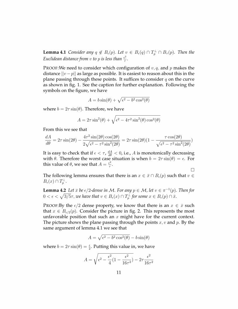
θ

ε

Ab

τq

pTp

Tp

v

Figure 1: A picture showing the worst case. The picture shows the planepassing through points v, p, and q. Tp and T⊥

p are shown intersecting withthis plane and are represented by the dotted horizontal line and the solidvertical line respectively. On the plane of interest, one may then draw twocircles (of radius τ each) that are tangent to Tp and are on either side ofTp as shown. Clearly v lies on T⊥

p and is marked in the figure. On theother hand q could potentially lie anywhere outside the two circles. Amoment’s reflection shows that ||v − p|| is greatest when q lies on one ofthe two circles. Without loss of generality one may consider it to lie on thetop circle as shown. Over all choices of such q, the worst case is derived inlemma 4.1

10

Lemma 4.1 Consider any q 6∈ Bε(p). Let v ∈ Bε(q) ∩ T⊥p ∩ Bτ (p). Then the

Euclidean distance from v to p is less than ε2

τ.

PROOF:We need to consider which configuration of v, q, and p makes thedistance ||v−p|| as large as possible. It is easiest to reason about this in theplane passing through these points. It suffices to consider q on the curveas shown in fig. 1. See the caption for further explanation. Following thesymbols on the figure, we have

A = b sin(θ) +√

ε2 − b2 cos2(θ)

where b = 2τ sin(θ). Therefore, we have

A = 2τ sin2(θ) +√

ε2 − 4τ 2 sin2(θ) cos2(θ)

From this we see that

dA

dθ= 2τ sin(2θ) − 4τ 2 sin(2θ) cos(2θ)

2√

ε2 − τ 2 sin2(2θ)= 2τ sin(2θ)(1 − τ cos(2θ)

√

ε2 − τ 2 sin2(2θ))

It is easy to check that if ε < τ , dAdθ

< 0, i.e., A is monotonically decreasingwith θ. Therefore the worst case situation is when b = 2τ sin(θ) = ε. Forthis value of θ, we see that A = ε2

τ.

¤

The following lemma ensures that there is an x ∈ x ∩ Bε(p) such that v ∈Bε(x) ∩ T⊥

p .

Lemma 4.2 Let x be ε/2-dense in M. For any p ∈ M, let v ∈ π−1(p). Then for

0 < ε <√

3/5τ, we have that v ∈ Bε(x) ∩ T⊥p for some x ∈ Bε(p) ∩ x.

PROOF:By the ε/2 dense property, we know that there is an x ∈ x suchthat x ∈ Bε/2(p). Consider the picture in fig. 2. This represents the mostunfavorable position that such an x might have for the current context.The picture shows the plane passing through the points x, v and p. By thesame argument of lemma 4.1 we see that

A =√

ε2 − b2 cos2(θ) − b sin(θ)

where b = 2τ sin(θ) = ε2. Putting this value in, we have

A =

√

ε2 − ε2

4(1 − ε2

16τ 2) − 2τ

ε2

16τ 2

11

Simplifying, we see that A > ε2

τ(needed by lemma 4.1) if

√

ε2 − ε2

4(1 − ε2

16τ 2) >

9

8

ε2

τ

Squaring both sides, we have

3

4ε2 +

ε4

64τ 2>

81ε4

64τ 2

This simplifies toε2

τ 2<

3

5

Therefore, as long as ε <√

35τ , we will have that v ∈ Bε(x) for a suitable x.

¤

5 Probability Bounds

Following our assumption, that the points xi are drawn at random, wenow provide a bound on how many examples need to be drawn so that theempirically constructed complex has the same homology as the manifold.We begin with a basic probability lemma.

Lemma 5.1 Let {Ai} for i = 1, . . . l be a finite collection of measurable sets andlet µ be a probability measure on ∪l

i=1Ai such that for all 1 ≤ i ≤ l, we haveµ(Ai) > α. Let x = {x1, . . . , xn} be a set of n i.i.d. draws according to µ. Then if

n ≥ 1

α

(

log l + log(1

δ)

)

we are guaranteed that with probability > 1 − δ, the following is true

∀i, x ∩ Ai 6= ∅

PROOF:This follows from a simple application of the union bound. Let Ei

be the event that x∩Ai is empty. The probability with which this happensis given by

IPEi = (1 − µ(Ai))n ≤ (1 − α)n.

12

����

��

��

q

pTp

Tp

bθ

εA

x

τv

Figure 2: A picture showing the worst case. The picture is of the planecontaining the points p, v, and x. The two circles are each of radius τ andtangent to Tp. Tp and T⊥

p are represented by their intersection with theplane of interest as dotted horizontal and solid vertical lines respectively.

13

Therefore, by the union bound, we have

IP∪iEi ≤l

∑

i=1

IPEi ≤ l(1 − α)n

It remains to show that for n ≥ 1α

(

log l + log(1δ))

, we have

l(1 − α)n ≤ δ

To see this, simply note that f(x) = xex − ex + 1 ≥ 0 for all x ≥ 0. Thisis seen by noting that f(0) = 0 and f ′(x) = xex ≥ 0 for all x ≥ 0. Puttingx = α in the above function, we have

(1 − α) ≤ e−α

and therefore it is easily seen that

l(1 − α)n ≤ le−nα ≤ δ

for the appropriate choice of n.¤

Applying this to our setting, we consider a cover of the manifold M byballs of radius ε

4. Let {yi; 1 ≤ i ≤ l} be the centers of such balls that consti-

tute a minimal cover. Therefore, we can choose Ai = B ε4(yi) ∩M. Apply-

ing the above lemma, we immediately have an estimate on the number ofexamples we need to collect. This is given by

1

α

(

log l + log(1

δ)

)

where

α = mini

vol(Ai)

vol(M)

and l is the ε4

covering number. These may be expressed entirely in termsof natural invariants of the manifold and we derive these quantities below.First, we note that the covering number may be bounded in terms of thepacking number, i.e., the maximum number of sets of the form Ni = Br ∩M (at scale r) that may be packed into M without overlap. In particular,if C(ε) is the ε-covering number of M and P (ε) is the ε-packing number,then the following simple lemma is true.

14

Lemma 5.2P (2ε) ≤ C(2ε) ≤ P (ε)

PROOF:The fact that P (2ε) ≤ C(2ε) follows from the definition. To see thatC(2ε) ≤ P (ε), begin by letting Bε(x1), . . . , Bε(xN) be a realization of an op-timal ε-packing so that N = P (ε). We claim that B2ε(x1), . . . , B2ε(xN) forma 2ε-cover. If not, there exists an x ∈ M such that Bε(x)∩Bε(xi) is empty forall i. In that case, one can add Bε(x) to the collection to increase the pack-ing number by 1 leading to a contradiction. Since B2ε(x1), . . . , B2ε(xN) is avalid 2ε-cover, we have C(2ε) ≤ N = P (ε).

¤

Since l is the ε/4 covering number, we see that l ≤ P (ε/8) from lemma 5.2.Now we need to bound the packing number. To do so, we need the fol-lowing result.

Lemma 5.3 Let p ∈ M. Now consider A = M ∩ Bε(p). Then vol(A) ≥(cos(θ))kvol(Bk

ε (p)) where Bkε (p) is the k-dimensional ball in Tp centered at p,

θ = arcsin( ε2τ

). All volumes are k-dimensional volumes where k is the dimensionof M.

PROOF:Consider the tangent space at p given by Tp and let f be the projec-tion of IRN to Tp. Let Bk

r (p) be the k-dimensional ball of radius r = ε cos(θ)(where θ = arcsin( ε

2τ)) centered at p lying in Tp. Let fA = {f(q) |q ∈ A}

be the image of A under f . We will show that Bkr (p) ⊂ fA. Since f is a

projection we have

vol(A) ≥ vol(fA) ≥ vol(Bkr (p)) = (cosk(θ))vol(Bk

ε (p))

To see that Bkr (p) ⊂ fA, notice that f is an open map whose derivative is

nonsingular for all q ∈ A (by Lemma 5.4). Therefore f is locally invertibleand there exists a ball Bk

s (p) of radius s such that f−1(Bks (p)) ⊂ A. One

can keep increasing s until it happens for the first time (say at s = s′) thatf−1(Bk

s (p)) 6⊂ A. At this stage, there exists a point q in the closure of Asuch either (i) f is singular at q or (ii) q 6∈ A. By Lemma 5.4, we see that (i)is impossible. Therefore, q 6∈ A but q is in the closure of A implying that‖q − p‖ = ε. We see that s′ = ε cos(φ) where φ is the angle between theline qp (the line joining q to p) and the line ¯f(q)p (the line joining f(q) to p).By the curvature bound implied by τ , we see that |φ| ≤ |θ| and therefores′ = ε cos(φ) ≥ ε cos(θ) = r. ¤

15

Lemma 5.4 Let p ∈ M, let A = M ∩ Bε(p), and let f be the projection to thetangent space at p (Tp). Then for all ε < τ

2, the derivative df is nonsingular at all

points q ∈ A.

PROOF:Suppose df was singular for some q ∈ A. That means that the tangentspace at q (Tq) is oriented so that the vector with origin q and end pointf(q) lies in Tq. Since q ∈ Bε(p), we have that d = ||q − p|| < τ

2. Putting

propositions 6.2 and 6.3 together, we get that

cos(φ) ≥√

1 − 2d

τ> 0

where φ is the angle between Tp and Tq. From this we see that φ < π2

leading to a contradiction.¤

Using lemma 5.3, we see that a simple bound on the packing number isobtained. We obtain immediately that

P (ε) ≤ vol(M)

(cosk(θ))vol(Bkε (p))

Therefore, we have

l ≤ P (ε

8) ≤ vol(M)

(cosk(θ2))vol(Bkε8

(p))

where θ2 = arcsin( ε16τ

). Similarly, we have that

1

α≤ vol(M)

(cosk(θ1))vol(Bkε4

(p))

where θ1 = arcsin( ε8τ

).

6 Curvature and the Condition Number 1τ

In this section1, we examine the consequences of the condition number1τ

for the submanifold M. As we have mentioned before, τ controls the

1Thanks to Nat Smale for discussions leading to the writing of this section.

16

curvature of the manifold at every point. This fact has been exploited inour earlier proofs. For submanifolds, one may formally study curvaturethrough the second fundamental form (see e.g., [14]). Here we show for-mally that the norm of the second fundamental form is bounded by 1

τ.

Thus a large τ corresponds to a well conditioned submanifold that haslow curvature.Proposition 6.1 states the bound on the norm of the second fundamentalform. Proposition 6.2 states a bound on the maximum angle between tan-gent spaces at different points in M. Proposition 6.3 states a bound onthe maximum difference between the geodesic distance and the ambientdistance for neighboring points in M.Let us begin by recalling the second fundamental form. Fix a point p ∈M. Following standard accounts (see, e.g. [14]), there exists a symmetricbilinear form B : Tp × Tp → T⊥

p that maps any two vectors in the tangentspace (u, v ∈ Tp) into a vector B(u, v) in the normal space. Thus for anynormal vector (unit norm) η ∈ T⊥

p , one can define the following

Bη(u, v) = 〈η,B(u, v)〉 = 〈u, Lηv〉

where the inner product 〈·, ·〉 is the usual inner product in the tangentspace of the ambient manifold (in our case IRN ). Since Bη : Tp × Tp → IRis symmetric and bilinear, we see that Lη : Tp → Tp is a linear self-adjointoperator. The norm of the second fundamental form in direction η is nowgiven by

λη = supu∈Tp

〈u, Lηu〉〈u, u〉

It is seen that λη is the largest eigenvalue of Lη. (In general, the eigenval-ues are also known as the principal curvatures in the normal direction η).Given this, we can prove the following proposition that characterizes therelation between the curvature through the second fundamental form andthe condition number of the submanifold.

Proposition 6.1 If M is a submanifold of IRN with condition number 1τ, then

the norm of the second fundamental form is bounded by 1τ

in all directions. Inother words, for all points p ∈ M and for all (unit norm) η ∈ T⊥

p , we have

λη = supu∈Tp

〈u, Lηu〉〈u, u〉 ≤ 1

τ

17

PROOF:We prove by contradiction. Suppose the proposition is false. Thenthere exists a point p ∈ M, a tangent vector (unit norm) u ∈ Tp and anormal vector (unit norm) η such that

〈η,B(u, u)〉 >1

τ

Consider a geodesic curve c(t) ∈ M parametrized by arc length such thatc(0) = p and c(0) = dc

dt(0) = u. For convenience, we will place the origin at

p so that c(0) = 0 = p. With this (ambient) coordinate system, consider thepoint given by τη, i.e., the point a distance τ from p in the direction η. Byour hypothesis on the condition number of the submanifold, we see thatp ∈ M is the closest point on the manifold to the center of the τ -ball givenby τη.

for all t, ||c(t) − τη||2 ≥ τ 2

from which we get

∀t, 〈c(t), c(t)〉 − 2τ〈c(t), η〉 ≥ 0

Consider the function g(t) = 〈c(t), c(t)〉− 2τ〈c(t), η〉. Since c(0) = 0, we seethat g(0) = 0. Further, we have g′(t) = 2〈c(t), c(t)〉−2τ〈c(t), η〉. Since c(0) =0 and 〈c(0), η〉 = 0, we see that g′(0) = 0. Finally, g′′(t) = 2〈c(t), c(t)〉 +2〈c(t), c(t)〉 − 2τ〈c(t), η〉. Since c is parameterized by arc length, we have〈c(t), c(t)〉 = 1 and g′′(0) = 2 − 2τ〈c(0), η〉.Noting that the tangent vector field dc

dtis parallel (see proof of Proposi-

tion 6.2), we see that B(dcdt

, dcdt

) = c(t). Therefore, by assumption, we havethat

〈η,B(u, u)〉 = 〈η,B(dc

dt,dc

dt)〉 = 〈η, c(0)〉 >

1

τ

Therefore, g′′(0) < 2 − 2τ( 1τ) = 0. By continuity, there exists a t∗ such that

g(t∗) < 0. But this leads to a contradiction since g(t) ≥ 0 for all t.¤

Since the norm of the second fundamental form is bounded, we see thatthe manifold cannot curve too much locally. As a result, the angle betweentangent spaces at nearby points cannot be too large. Let p and q be twopoints in the submanifold M with associated tangent spaces Tp and Tq.Since Tp and Tq are affine subspaces of IRN , one can compare them in theambient space in a standard way.

18

Formally, one may transport the tangent spaces to the origin (accordingto the standard connection defined in the ambient space IRN ) and thencompare vectors in each of these tangent spaces with each other. Thus forany (unit norm) vectors u ∈ Tp and v ∈ Tq, we may define the angle θbetween them by

cos(θ) = |〈u′, v′〉|where 〈·, ·〉 is the usual inner product in IRN , u′, v′ are the vectors obtainedby parallel transport (in IRN ) of u and v respectively to the origin. Here-after, we will always take this construction as standard. We will drop theprime notation and use 〈u, v〉 to denote 〈u′, v′〉 in what follows.We can now state the following proposition.

Proposition 6.2 Let M be a submanifold of IRN with condition number 1τ. Let

p, q ∈ M be two points with geodesic distance given by dM(p, q). Let φ be the theangle between the tangent spaces Tp and Tq defined by cos(φ) = minu∈Tp maxv∈Tq |〈u, v〉|.Then cos(φ) is greater than 1 − 1

τdM(p, q).

PROOF:Consider two points p, q ∈ M connected by a geodesic curve c(t) ∈M. Let c(t) be parametrized (proportional to arc length) so that c(0) = p,and c(1) = q.Now let vp ∈ Tp be a tangent vector (unit norm) and let v(t) be the paralleltransport of this vector along the curve c(t). Thus we have v(0) = vp,v(1) = vq ∈ Tq. Clearly 〈v(t), v(t)〉 = 1 for all t since v is parallel.Notice that

〈v(0), v(1)〉 = 〈v(0), v(0) + w〉 = 1 + 〈v(0), w〉 (1)

where

w =

∫ 1

0

(dv

dt)dt (2)

Combining 1 and 2, we see

cos(θ) = |〈v(0), v(1)〉| ≥ 1 − |〈v(0), w〉| ≥ 1 − ||w|| (3)

where θ is the angle between the vectors v(0) and v(1). Since vp = v(0) wasarbitrary, it is easy to check that cos(φ) ≥ cos(θ).Now

dv

dt= ∇ dc

dtv(t)

19

where ∇ denotes the connection in Euclidean space. At the same time

∇ dcdt

v(t) = (∇ dcdt

v(t))T

where for any r ∈ M and v ∈ Tr (here Tr is the tangent space of IRN atr) we denote by (v)T the projection of v onto Tr (here Tr is the tangentspace to M at r viewed as an affine space with origin r). But since v(t)is parallel, we have that ∇ dc

dtv(t) = 0. Therefore, ∇ dc

dtv(t) is entirely in the

space normal to Tc(t). But the component of ∇ dcdt

v(t) in the normal direction

is precisely given by the second fundamental form. Hence, we have that

dv

dt= B(

dc

dt, v(t))

where B is a symmetric, bilinear form (the second fundamental form).Letting η be a unit norm vector in the direction dv

dt, i.e., η = (1/||dv

dt||)dv

dt, we

see that

||dv

dt|| = 〈η,

dv

dt〉 = 〈η,B(

dc

dt, v(t))〉 = 〈dc

dt, Lnv(t)〉

where Ln is a self adjoint linear operator. By Proposition 6.1, the norm ofLη is bounded by 1

τ. Therefore, we have

‖dv

dt‖ ≤ ‖dc

dt‖‖Lnv‖ ≤ ‖dc

dt‖‖Lη‖

and

‖w‖ = ‖∫ 1

0

dv

dt‖ ≤

∫ 1

0

‖dv

dt‖ ≤ ‖Ln‖

∫ 1

0

‖dc

dt‖dt ≤ 1

τdM(p, q) (4)

Combining eq. 3 and eq. 4, we get

cos(φ) ≥ 1 − 1

τdM(p, q)

¤

We next show a relationship between the geodesic distance dM(p, q) andthe ambient distance ||p− q||IRN for any two points p and q on the subman-ifold M.

20

Proposition 6.3 Let M be a submanifold of IRN with condition number 1τ. Let

p and q be two points in M such that ||p − q||IRN = d. Then for all d ≤ τ2, the

geodesic distance dM(p, q) is bounded by

dM(p, q) ≤ τ − τ

√

1 − 2d

τ

PROOF:Consider two points p, q ∈ M and let c(t) be a geodesic curve join-ing them such that c(0) = p and c(s) = q. Let c be parametrized by arclength so that ||c(t)|| = 1 for all t and dM(p, q) = s.Noting that the tangent vector field c along the curve is parallel, we havec = B(c, c) and from proposition 6.1, we see that for all t

||c|| = ||B(c, c)|| ≤ 1

τ

The chord length between p and q is given by ||c(s) − c(0)|| and we nowrelate this to the geodesic distance dM(p, q). Observe that

c(s) − c(0) =

∫ s

0

c(t)dt

Now

c(t) = c(0) +

∫ t

0

c(r)dr

Thus c(t) = c(0) + u(t) where u(t) =∫ t

0c(r)dr. We see that

||u(t)|| ≤∫ t

0

||c(r)dr|| ≤ t

τ

Therefore,

||c(s)−c(0)|| = ||∫ s

0

c(0)dt+

∫ s

0

u(t)dt|| ≥ s||c(0)||−∫ s

0

||u(t)||dt ≥ s−∫ s

0

t

τdt

Therefore we get

||c(s) − c(0)|| = d ≥ s − s2

2τ(5)

21

where d is the ambient distance between the points p and q while s is thegeodesic distance between these same points. The inequality in eq. 5 is

satisfied only if s ≤ τ − τ√

1 − 2dτ

or s ≥ τ + τ√

1 − 2dτ

. Since s = 0 when

d = 0, we know that the second inequality does not apply. Therefore, fromthe first inequality, we have

s ≤ τ − τ

√

1 − 2d

τ

¤

7 Handling Noisy Data

In this section we show that if our data is noisy in the sense that it is drawnfrom a probability distribution that is concentrated around (rather thanon) the manifold, the homology of the manifold can still be computed fromnoisy data.

7.1 The Model of Noise

Consider a probability measure µ concentrated around the manifold. Weassume that µ satisfies the following two regularity conditions.

1. The support of µ (suppµ) is contained in the tubular neighborhoodof radius r around M. Thus suppµ ⊂ Tubr(M).

2. For every 0 < s < r, we have that

infp∈M

µ(Bs(p)) > ks

where ks is a constant depending on s and independent of p.

In what follows, we assume the data is drawn in i.i.d. fashion accordingto a P that satisfies the above properties.

22

7.2 Main Topological Lemma: Sufficient Conditions

We will proceed by constructing ε-balls centered on our data points. Ifthese data are s-dense on the manifold, then the homology of the unionof these balls will equal that of the manifold M even if the data is drawnfrom a noisy distribution. In order to see that this might be the case at all,we provide a simple argument. This argument works with non-optimalchoices of ε and s and later sections will enter into the considerations ofchoosing better values for these parameters and therefore provide morenatural complexity estimates.Let x = {x1, . . . , xn} be a set of n points in the tubular neighborhood ofradius r around M. Let U be given by

U = ∪x∈xBε(x)

Proposition 7.1 If x is r-dense in M then M is a deformation retract of U for

all r < (√

9 −√

8)τ and ε ∈(

(r+τ)−√

r2+τ2−6τr2

, (r+τ)+√

r2+τ2−6τr2

)

.

PROOF:We show that for each p ∈ M, it is the case that π−1(p) contractsto p. Consider a v ∈ π−1(p). Consider the line segment, vp, joining v to p.We claim that this line segment is entirely contained in π−1(p). Clearly, ifv ∈ Bε(x) for some x ∈ x ∩ Bε(p), this is immediate by the convexity ofballs in Euclidean space. So we only need to consider the situation wherev ∈ Bε(x) for some x 6∈ x ∩ Bε(p). So let v ∈ Bε(q) ∩ T⊥

p . Let

u = arg minx∈vp∩ ¯Bε(q)

||x − p||

As long as u ∈ Bε(x) for some x ∈ x ∩ Bε(p), we see that the line segmentup is contained in π−1(p) and therefore v contracts to p.Since we choose r < ε, we are guaranteed that there is an x ∈ x ∩ Br(p) ⊂Bε(p). The worst case picture is shown in fig. 3. Following the symbols ofthe picture, as long as

τ − A < ε − r,

we have that v contracts to p. Thus we need

(τ − (ε − r))2 < A2 = (τ − r)2 − ε2 (6)

Expanding the squares, this reduces to

ε2 − ε(τ + r) + 2τr < 0

23

This is a quadratic in ε and is satisfied for

ε ∈(

(r + τ) −√

r2 + τ 2 − 6τr

2,(r + τ) +

√r2 + τ 2 − 6τr

2

)

(7)

providedr2 − 6τr + τ 2 > 0

This, in turn, is a quadratic in r and it is easy to check that it is satisfied aslong as

r < (3 − 2√

2)τ = (√

9 −√

8)τ (8)

Thus we see that for r, ε satisfying equations 7 and 8, we have that vcontracts to p. ¤

We now need to compute the probability of drawing a random x that isguaranteed to be r-dense. The following proposition is true.

Proposition 7.2 Let Nr/2 be the r/2-covering number of the manifold. Let p1, . . . , pNr/2∈

M be points on the manifold such that Br/2(pi) realize an r/2-cover of the mani-fold. Let x be generated by i.i.d. draws according to a probability measure µ thatsatisfies the regularity properties described earlier. Then if |x| > 1

kr/2

(

log(Nr/2) + log(1δ))

,

with probability greater than 1 − δ, x will be r-dense in M.

PROOF:Take Ai = Br/2(pi) and apply Lemma 5.1. By the conclusion of thatlemma, we have that with high probability each of the Ai’s is occupied byatleast one x ∈ x. Therefore it follows that for any p ∈ M, there is atleastone x ∈ x such that ||p − x|| < r. Thus with high probability x is r-denseon the manifold.

¤

Putting these together, our main conclusion is

Theorem 7.1 Let Nr/2 be the r/2-covering number of the submanifold M ofIRN . Let x be generated by i.i.d. draws according to a probability measure µthat satisfies the regularity properties described earlier. Let U = ∪x∈xBε(x).Then if |x| > 1

kr/2

(

log(Nr/2) + log(1δ))

, with probability greater than 1 − δ,

M is a deformation retract of U as long as (1) r < (√

9 −√

8)τ and (2) ε ∈(

(r+τ)−√

r2+τ2−6τr2

, (r+τ)+√

r2+τ2−6τr2

)

24

��

����

����

����

pTp

T

qε

τ

r

p

A

x

v

Figure 3: A picture showing the worst case. As before, we draw the picturein the plane connecting points v, p, and q. Tp and T⊥

p are intersected withthis plane in the picture and shown by the dotted horizontal line and solidvertical line respectively. The concentric circles have the same center andare of radius τ and τ − r respectively and follow our usual construction inearlier figures and arguments. All lengths are marked by arrows.

25

7.3 Main Topological Lemma – General Considerations

In general, we may demand points that are s-dense. Putting ε-balls aroundthese points we construct U in the usual way. The condition number τ andthe noise bound r are additional parameters that are outside our controland determined externally. We now ask what is the feasible space (s, ε, r, τ)that will guarantee that U is homotopy equivalent to M?Following our usual logic, we see that the worst case situation is given byfig. 4. An arbitrary v ∈ Bε(q) ∩ T⊥

p ∩ Bτ (p) will contract to p if

Bε(q) ∩ Bε(x) ∩ vp 6= φ

This is the same as requiring

(τ − w)2 < (τ − r)2 − ε2 (9)

Additionally, we have the following equations that need to be satisfied(following fig. 4).

(τ − r)2 − (τ − β)2 = s2 − β2 (10)

s2 − β2 + (β + w)2 = ε2 (11)

If one eliminates w and β from the above equations, one will get a singleinequality relating s, ε, τ, r that describes for each τ, r the feasible set ofpossible choices of s, ε that are sufficient to guarantee homotopy equiva-lence. Let us see how our earlier theorems follow from particular choicesof this general set of equations.

7.3.1 The Case when s = r

We have already examined the case when the points x are chosen to ber-dense in M. Putting in s = r in equations 9, 10, and 11, we see thefollowing:From eq. 10, we have (for s = r)

(τ − r)2 − (τ − β)2 = r2 − β2

This simplifies to give β = r.Putting β = r and s = r in eq. 11, we get

r2 − r2 + (r + w)2 = ε2

26

����

����

����

����

Tp

T

qε

τ

p

A

pr

ε

β

x

τ−r

v

w

Figure 4: A picture showing the worst case. As before, we draw the picturein the plane connecting points v, p, and q. Tp and T⊥

p are intersected withthis plane in the picture and shown by the dotted horizontal line and solidvertical line respectively. The concentric circles have the same center andare of radius τ and τ − r respectively and follow our usual construction inearlier figures and arguments. All lengths are marked by arrows.

27

giving us w = ε − r.Finally, putting w = ε − r in inequality 9, we get

(τ − (ε − r))2 < (τ − r)2 − ε2

which is the same as inequality 6 whose solution was examined in theprevious section.

7.3.2 The Case when r = 0

We can recover our main theorem for the noise-free case by consideringthe case r = 0. We proceed to do this now.The fundamental inequality of 9 gives us (for r = 0)

(τ − w)2 < τ 2 − ε2

This is the same as requiring

w2 − 2τ + ε2 < 0

Using standard analysis for quadratic functions, we see that the followingcondition is required:

w > τ −√

τ 2 − ε2 (12)

We can eliminate w using equations 10 and 11. Thus, from eq. 10, we get

β = s2

2τand substituting in eq. 11, we get a quadratic equation in w whose

positive solution is given by w = − s2

2τ+

√

s4

4τ2 + (ε2 − s2). This gives rise to

the following condition

− s2

2τ+

√

s4

4τ 2+ (ε2 − s2) > τ −

√τ 2 − ε2 (13)

Inequality 13 gives the feasible region for s and ε for the homotopy equiv-alence of U and M. Let us consider the special case when s = ε

2— a choice

we made in Section 3 without any attention to optimality. Putting in thisvalue, after several simplifying steps, one obtains that

ε4 + 51ε2τ 2 − 48τ 4 < 0 (14)

This is satisfied for all 0 < ε2 < 0.9244τ 2 or

0 < ε < 0.96τ

28

Remark 1 Note that in our original proof of our main noise free theo-rem (Theorem 3.1), the deformation retract argument of Section 3 passesthrough the construction of st(p) and shows contraction of π−1(p) by equat-ing it with st(p). This condition is stronger than we require. Here we seethat the condition Bε(q)∩Bε(x)∩ vp 6= φ is sufficient. This latter conditionis weaker and therefore gives us a slightly stronger version of Theorem 3.1in the sense that it holds for a larger range of ε.Remark 2 If we assume that τ, r are beyond our control, the sample com-plexity depends entirely upon s. Therefore if we wish to proceed by draw-ing the fewest number of examples, then it is necessary to maximize s sub-ject to the condition of eq. 13.Remark 3 The total complexity of finding the homology depends bothupon s and ε in a more complicated way. The size of x depends entirelyupon s and nothing else. However, the number of k-tuples to consider inthe simplicial complex depends both upon the size of x as well as ε becauseε determines how many balls will have non-empty intersections. We leavethis more nuanced complexity analysis for future consideration.

References

[1] N. Amenta and M. Bern. Surface reconstruction by Voronoi filtering.Discrete and Computational Geometry. Vol. 22. 1999.

[2] N. Amenta, S. Choi, T.K. Dey, and N. Leekha. A simple algorithm forhomeomorphic surface reconstruction. International Journal of Com-putational Geometry Applications. Vol. 12. 2002.

[3] S.W. Cheng, T.K. Dey, and E.A. Ramos. Manifold reconstruction frompoint samples. Proc. of ACM SIAM Symposium on Discrete Algo-rithms. 2005.

[4] F. Chazal and A. Lieutier. Weak feature size and persistent homol-ogy: computing homology of solids in IRn from noisy data samples.Preprint.

[5] H. Edelsbrunner and E.P. Mucke. Three-dimensional alpha shapes.ACM Transactions on Graphics. Vol. 13. 1994.

29

[6] D. Cohen-Steiner, H. Edelsbrunner and J. Harer. Stability of per-sistence diagrams. Proc. 21st Symposium Computational Geometry.2005.

[7] A. Zomorodian and G. Carlsson. Computing persistent homology.20th ACM Symposium on Computational Geometry, Brooklyn, NY,June 9-11, 2004.

[8] J. B. Tenenbaum, V. De Silva, J. C. Langford. A global geomet-ric framework for nonlinear dimensionality reduction. Science 290(5500): 22 December 2000.

[9] M. Belkin and P. Niyogi. Semisupervised Learning on RiemannianManifolds. Machine Learning. Vol. 56. 2004.

[10] A. Bjorner. Topological Methods. in “Handbook of Combinatorics”,(Graham, Grotschel, Lovasz (ed.)), North Holland, Amsterdam, 1995.

[11] S. T. Roweis and L. K. Saul. Nonlinear dimensionality reduction bylocally linear embedding. Science 290: 2323-2326.2000.

[12] D. Donoho and C. Grimes. Hessian Eigenmaps: New Locally-LinearEmbedding Techniques for High-Dimensional Data. Preprint. Stan-ford University, Department of Statistics. 2003.

[13] T. K. Dey, H. Edelsbrunner and S. Guha. Computational topology.Advances in Discrete and Computational Geometry, 109-143, eds.: B.Chazelle, J. E. Goodman and R. Pollack, Contemporary Mathematics223, AMS, Providence, 1999.

[14] M. P. Do Carmo. Riemannian Geometry. Birkhauser. 1992.

[15] J. Munkres. Elements of Algebraic Topology. Perseus Publishing.1984.

[16] J. Friedman. Computing Betti Numbers via the Combinatorial Lapla-cian. Algorithmica. 21. 1998.

[17] K. Fischer, B. Gaertner, M. Kutz. Fast Smallest-Enclosing-Ball Compu-tation in High Dimensions. Proc. 11th Annual European Symposiumon Algorithms (ESA), 2003.

30

[18] Website for Smallest Enclosing Ball Algorithm.http://www2.inf.ethz.ch/personal/gaertner/miniball.html

[19] T. Kaczynski, K. Mischaikow, M. Mrozek. Computational Homology.Springer Verlag, NY. Vol. 157. 2004.

[20] L. G. Valiant. A Theory of the Learnable. Communications of theACM. Vol. 27, Issue 11. 1984.

31