finding spin glass ground states using quantum walksfinding spin glass ground states using quantum...

Finding spin glass ground states using quantumwalks

Adam Callison1, Nicholas Chancellor2, Florian Mintert1

and Viv Kendon2

1 Blackett Laboratory, Imperial College London, London SW7 2BW, UK2 Physics Department, Durham University, South Road, Durham, DH1 3LE, UK

E-mail: [email protected], [email protected]

Abstract. Quantum computation using continuous-time evolution under anatural hardware Hamiltonian is a promising near- and mid-term direction towardpowerful quantum computing hardware. We investigate the performance ofcontinuous-time quantum walks as a tool for finding spin glass ground states,a problem that serves as a useful model for realistic optimization problems.By performing detailed numerics, we uncover significant ways in which solvingspin glass problems differs from applying quantum walks to the search problem.Importantly, unlike for the search problem, parameters such as the hopping rateof the quantum walk do not need to be set precisely for the spin glass groundstate problem. Heuristic values of the hopping rate determined from the energyscales in the problem Hamiltonian are sufficient for obtaining a better quantumadvantage than for search. We uncover two general mechanisms that providethe quantum advantage: matching the driver Hamiltonian to the encoding inthe problem Hamiltonian, and an energy redistribution principle that ensures aquantum walk will find a lower energy state in a short timescale. This makes itpractical to use quantum walks for solving hard problems, and opens the door fora range of applications on suitable quantum hardware.

Keywords: quantum computing, quantum walks, spin glasses

arX

iv:1

903.

0500

3v3

[qu

ant-

ph]

20

Dec

201

9

Quantum walk spin glass ground states 2

Contents

1 Introduction 2

2 Computing with quantum walks 52.1 Continuous-time quantum walks . . . . . . . . . . . . . . . . . . . . . 52.2 Computing using a quantum walk . . . . . . . . . . . . . . . . . . . . 62.3 Graph choice for quantum walk computing . . . . . . . . . . . . . . . 72.4 Solving the search problem using quantum walks . . . . . . . . . . . . 8

3 Spin glass problem definitions 103.1 Sherrington-Kirkpatrick spin glass . . . . . . . . . . . . . . . . . . . . 113.2 Random energy model . . . . . . . . . . . . . . . . . . . . . . . . . . . 12

4 Numerical methods 12

5 Quantum walks with spin glasses 135.1 Setting the hopping rate . . . . . . . . . . . . . . . . . . . . . . . . . . 135.2 Success probability . . . . . . . . . . . . . . . . . . . . . . . . . . . . . 165.3 Mixing times . . . . . . . . . . . . . . . . . . . . . . . . . . . . . . . . 19

6 Computational mechanisms 216.1 Role of correlations in SK . . . . . . . . . . . . . . . . . . . . . . . . . 216.2 Energy conservation dynamics . . . . . . . . . . . . . . . . . . . . . . . 23

7 Summary and outlook 24

1. Introduction

Optimization problems need to be solved in a broad range of areas, such as scheduling,route planning, supply chains, finance. This is often computationally intensive, so theprospect of quantum enhanced solution methods is an important research direction forpractical quantum computing. One way to tackle optimization in a quantum setting isto use a device which realises an Ising Hamiltonian with a transverse field. Computingusing the Ising Hamiltonian works as follows: The optimization problem is encodedinto the Ising Hamiltonian HI

HI = −n−1∑

(j 6=k)=0

JjkZjZk −n−1∑j=0

hjZj , (1)

on n qubits, such that the solution corresponds to the ground state of HI . In ournotation, the operator Zj on the full Hilbert space applies the single qubit Pauli-Z

operator Z to the jth qubit,

Zj =

(j−1⊗r=0

12

)⊗ Z ⊗

n−1⊗r=j+1

12

, (2)

where 12 is the identity operator on a single qubit. The (real) values of the couplingstrengths Jjk and fields hj define the optimization problem, and efficient methods


are known for expressing optimization problems in terms of these coupling and fieldstrengths (e.g., Choi, 2010). The transverse field term HT

HT = −Γ

n−1∑j=0

Xj , (3)

drives transitions between states, where Γ is a real-valued transverse field strength,and Xj is the operator on the full Hilbert space that applies the single qubit Pauli-X

operator to the jth qubit, defined by analogy with Zj in (2). The qubits are initialised

in the ground state of HT , this is easy to do by applying a strong transverse field toalign all the qubits in the state |+〉 = 2−1/2(|0〉 + |1〉). Then, the computation iscarried out by applying the full transverse Ising Hamiltonian

HTI(t) = A(t)HT +B(t)HI , (4)

where t is time and A(t), B(t) are real-valued control functions. To obtain a candidatesolution to the optimization problem, the qubit register is measured after a time tf .For some problems, sampling from the distribution of low energy states provides therequired solution – this can be done by repeating the computation, which will ingeneral not produce the lowest energy state with certainty.

The Ising Hamiltonian is a natural choice for encoding problems for two reasons.First, it is proven to be universal for classical problems (De las Cuevas and Cubitt,2016). There are efficient methods for mapping NP-hard optimization problems tothe Ising model (Lucas, 2014; Choi, 2010), providing a practical route to quantumalgorithms. Since many optimization problems are NP-hard, an exponential speed upis not expected, but even modest polynomial improvements are useful for practicalapplications. There is increasing interest in how to obtain polynomial advantagesthrough quantum algorithms (Moylett et al., 2017; Montanaro, 2018; Ambainis et al.,2019). Interesting results have been presented for a wide range of applications, suchas mathematics (Bian et al., 2013; Li et al., 2017), computer science (Chancelloret al., 2016), computational biology (Perdomo-Ortiz et al., 2012), finance (Marzec,2016), and aerospace (Coxson et al., 2014). Second, the Ising Hamiltonian can beimplemented in a range of different physical systems. The quantum Ising Hamiltonianis the basic interaction Hamiltonian in the D-Wave Systems Inc. programmablesuperconducting devices (D-Wave, 1999–; Boixo et al., 2013; Johnson et al., 2011).Implementations in other promising architectures include Rydberg systems (Bernienet al., 2017) and trapped ions (Kim et al., 2011). The Ising Hamiltonian isalso the basic tool for specialised optimization hardware, such as coherent Isingmachines (Inagaki et al., 2016; McMahon et al., 2016). Optimization using theIsing Hamiltonian can be implemented in digital quantum architectures by using thequantum approximate optimization algorithm (QAOA) (Farhi et al., 2014a,b; Marshand Wang, 2019) or quantum alternating operator ansatz (Hadfield et al., 2019).Studies by Zhou et al. (2018) show how to exploit non-adiabatic effects in QAOAon early quantum hardware.

There are several known methods for driving the quantum system from its initialstate into the ground state of a Hamiltonian defining the problem to be solved. Thesemethods correspond to different choices for the control functions A(t) and B(t) in (4).Adiabatic quantum computing (Kadowaki and Nishimori, 1998; Farhi et al., 2000,2001) keeps the quantum system in the ground state while the initial Hamiltonianis slowly changed into the problem Hamiltonian. Quantum annealing (Finnila et al.,1994) takes advantage of open quantum systems effects to cool the system towards


the ground state. Continuous-time quantum walks evolve the system under a time-independent Hamiltonian for a suitable time before measurement of the final state.Computation by continuous-time quantum walk and adiabatic quantum computingare end points of a family of continuous-time protocols that use the same Hamiltonianterms but are applied with different time dependent modulation (Morley et al., 2019).In this work, we focus on computation by quantum walk using time-independenttransverse Ising Hamiltonians.

Quantum walks can solve the search problem (Childs and Goldstone, 2004),achieving the same quadratic O(N1/2) quantum speed up as is obtained by Grover’salgorithm (Grover, 1996). We describe the search problem further in Subsection 2.4.For particular graphs, quantum walks can solve problems exponentially faster (e.g.,Childs et al., 2003), and quantum walks are now widely used as subroutines in morecomplex quantum algorithms. However, in the continuous-time setting, the applicationof quantum walks to optimization problems has not been studied in detail. There isincreasing interest in quenches (Amin et al., 2018) or pauses (Marshall et al., 2019;Passarelli et al., 2019) in quantum annealing, which effectively run an open-systemversion of a quantum walk during part of the computation. Thermal relaxation effectsdominate in the regime currently accessible by flux qubit quantum annealers, which isthe focus of these works. An algorithm which is essentially a quantum walk on a spinglass, although presented using different terminology, has been analysed by Hastings(2019). Along with the same energy conservation arguments we describe in section6.2, Hastings’ findings suggest that quantum walks on spin glasses will be interestingto explore. Given that quantum walks provide a better performance for searchingthan adiabatic quantum computing, especially when limited coherence time and otherpractical factors, such as precision of control settings, are considered (Morley et al.,2019), it is important to understand how they perform for a wider range of problems.

In this work, we tackle the question of if, and how, a quantum walk can be usefulfor practical quantum optimization. We present a detailed numerical investigationof continuous-time quantum walks applied to solving combinatorial optimizationproblems, using the Sherrington-Kirkpatrick spin glass ground state problem asa prototypical example. Finding the ground state of a frustrated Sherrington-Kirkpatrick spin glass (Sherrington and Kirkpatrick, 1975) is known to be not onlyNP-hard, but also uniformly-hard, as suggested by its finite-temperature spin glasstransition. Without a finite temperature spin glass transition, a problem cannot beuniformly hard, since the lack of a transition implies that typical cases will be easyfor the Monte Carlo family of algorithms, as discussed in (Katzgraber et al., 2014).As has been shown for a random problem type used in early benchmarks of quantumannealing hardware (Katzgraber et al., 2014), uniform hardness is crucial: withoutthis property, randomly generated instances of NP-hard problems are not necessarilyhard to solve (Beier and Vocking, 2004; Krivelevich and Vilenchik, 2006; Lucas, 2014).

We use a random energy model (Derrida, 1980) for comparisons, to draw out theeffects of the correlations between energy difference and Hamming distance in the spinglass. A problem with perfect correlations is easy to solve, like finding the ground stateof a spin system with only local fields, no couplings. A completely random problem,such as finding the ground state of a random energy model instance, has no correlationto exploit and so is very hard to solve, essentially requiring random guessing. However,a completely random model is fully characterised by average values of its properties,and finding exact ground states of specific instances is typically not interesting.Intermediate problems with some correlations are both hard and interesting, with


complex behaviour and phase diagrams, like spin models with frustration and spinglass phases. Real optimization problems typically have correlations; they are oftenhard to solve but also produce interesting solutions. The inherent complexity ofa problem comes from the structures of the problem and its correlations, not thestructure of the solution itself. One illustration of this is the construction of hardbenchmarking problems with ‘planted’ solutions defined at the time of construction,which therefore have no special structure related to the problem’s hardness, see forexample (Hen, 2019; Hamze et al., 2019).

The paper is structured as follows: In section 2, we review the settingfor computation by continuous-time quantum walk encoded into qubits, includingapplication to the search problem. In section 3, we introduce the Sherrington-Kirkpatrick spin glass model, and the random energy model we use for comparison.In section 4, we describe the numerical methods used in this investigation. In section5, we present the main results showing how quantum walks can find spin glass groundstates more effectively than a quantum search algorithm. In section 6, we identifythe computational mechanisms and important aspects of the problem structure thatcontribute to the effectiveness of quantum walk computation. Finally, in section 7, wesummarize and conclude.

2. Computing with quantum walks

Both discrete (coined) quantum walks (Aharonov et al., 2001; Shenvi et al., 2003) andcontinuous-time quantum walks (Farhi and Gutmann, 1998; Childs et al., 2003) areused for computation. This work only uses the continuous-time quantum walk, andalso only as an encoded quantum walk, in which qubits are used to store the binarylabels of the positions of the quantum walker (see figure 1 for a simple example).

2.1. Continuous-time quantum walks

A continuous-time quantum walk is defined on an undirected graph G(V,E), withV = {j}N−1

j=0 the set of N vertex labels and E the set of label-pairs (j, k) associatedwith edges. The vertices correspond to the positions of the walker, and the edgesindicate the allowed transitions between vertices. This is conveniently encoded in theadjacency matrix A of the graph, which has entries Ajk = 1 for (j, k) ∈ E and Ajk = 0otherwise. The Laplacian of G is L = A − D, where D is a diagonal matrix formedfrom the degree of each vertex, Djj = deg(j), where deg(j) is the number of edgesconnected to vertex j. Both the adjacency matrix A and Laplacian L are symmetricmatrices which can thus be used to define a quantum Hamiltonian for the dynamics ofthe continuous-time quantum walk on the graph. In this work, we only need regulargraphs, for which deg(j) is constant with respect to j. For regular graphs, the onlydifference between using the adjacency matrix A or Laplacian L is an irrelevant globalphase (Childs and Goldstone, 2004). We use the Laplacian form of the Hamiltonianfor consistency with prior work. We thus define the quantum walk Hamiltonian HG

for a quantum walk on graph G by

〈j| HG |k〉 = −γLjk, (5)

where γ is the hopping rate between connected vertices per unit time. The states|j〉 , |k〉 for j, k ∈ V are associated with the vertices of G and form a basis for a Hilbertspace of dimension N . In the Ising model context, the dimension of the Hilbert space


is N = 2n where n is the number of qubits, and {|j〉}N−1j=0 is the computational basis.

For a quantum walk starting in state |ψ(0)〉, the state of the walker evolves accordingto the Schrodinger equation, with formal solution

|ψ(t)〉 = exp{−iHGt} |ψ(0)〉 , (6)

using units in which ~ = 1.

2.2. Computing using a quantum walk

The task is to solve an optimization problem whose N = 2n candidate solutions j arerepresented in the computational basis {|j〉}N−1

j=0 , where j is a bit string corresponding

to the state of n qubits. The problem is encoded in an Ising Hamiltonian HP , ofthe form described by HI in (1) and whose eigenbasis is the computational basis. We

write the basis state with eigenvalue E(P )a as

∣∣∣E(P )a

⟩, with a ∈ {0 . . . N−1}, and adopt

the convention that E(P )a ≤ E

(P )a+1. In other words,

{ ∣∣∣E(P )a

⟩}N−1

a=0is a reordering of

{|j〉}N−1j=0 based on the corresponding eigenenergies of HP . The encoding is chosen such

that the solution corresponds to the ground state∣∣∣E(P )

0

⟩of the problem Hamiltonian

HP .To use a quantum walk to solve the problem, we must first choose a suitable state

in which to initialize the system. With no prior knowledge of the solution, the equalsuperposition of all basis states

|ψ(0)〉 = N−1/2N−1∑j=0

|j〉 , (7)

is a sensible choice that avoids bias. More generally, the initial state can be preparedas weighted or biased superposition, to incorporate prior knowledge about the solution(Perdomo-Ortiz et al., 2011; Duan et al., 2013; Chancellor, 2017; Graß and Lewenstein,2017; Baldwin and Laumann, 2018; Kechedzhi et al., 2018; Graß, 2019). Next, wechoose a suitable walk graph G. The main requirement is that the ground state ofthe quantum walk Hamiltonian HG coincides with the initial state, either biased orunbiased (see section 6.2). A simple way to achieve a biased starting state would beto ‘tilt’ the driver fields so they are no longer completely transverse. We only treatthe unbiased case in this work, so our initial state will be |ψ(0)〉 throughout. Thefull Hamiltonian H(γ) is defined by adding the quantum walk Hamiltonian HG to theproblem Hamiltonian HP

H(γ) ≡ HG + HP , (8)

where the key parameter is the hopping rate γ in HG, see (5). The computation isperformed by evolving the initial state (7) under the full Hamiltonian H(γ) for a timetf , then measuring the qubit register in the computational basis. The intuition, basedon the faster spreading of quantum walks over classical found in prior work (Farhiand Gutmann, 1998), is that the quantum walk dynamics provide rapid explorationof the basis states, while the energy structure of the problem Hamiltonian HP causeslocalisation around low-energy states.

The success probability P (tf ) =∣∣∣⟨E(P )

0

∣∣∣ψ(tf )⟩∣∣∣2 of finding the solution state

when measuring will not in general be unity. It will typically be necessary to repeat the


protocol multiple times to obtain a high probability of success over all the repeats. Ingeneral, it will be best to use different measurement times tf for each repeat. Differentmeasurement times will produce different success probabilities P (tf ), and varying themeasurement time avoids repeatedly measuring at a time for which the probabilityP (tf ) happens to be atypically small. More precisely, we choose the measurementtime tf uniformly at random in an interval [t, t+∆t], and define an average single runsuccess probability

P (t,∆t) ≡ 1

∆t

t+∆t∫t

dtfP (tf ). (9)

Operationally, choosing the measurement time tf randomly in the interval [t, t + ∆t]samples success probabilities from the distribution with P (t,∆t) as its mean. Samplingmeasurement times in this way means that the protocol typically needs to be repeatedMrep ∼ 1/P (t,∆t) times to achieve an overall O(1) success probability. Note that itis not generally possible to check whether the state measured is indeed the groundstate of HP . However, it is easy to calculate the energy of the state measured ineach repeat. If only the lowest energy state is accepted, it is only necessary for theground state of HP to be measured once out of all the repeats. The more repeats,the more confidence is gained that the lowest energy state found is the ground state.And studying the distribution of the sampled energies can provide more informationabout the problem.

The procedure described in this subsection does not in general provide an optimalquantum algorithm, because the repeats do not use information gained from theoutcomes of previous runs. We will discuss this further in section 7; for most of thispaper we are concerned with understanding the average single run success probability,as an essential prerequisite to building optimal algorithms.

In the limit of small interval width ∆t, the average success probability defined in(9) reduces to the single time probability P (tf ) = lim∆t→0 P (tf ,∆t). The long timelimit of this average,

P∞ ≡ P (0,∞) ≡ lim∆t→∞

P (0,∆t), (10)

is particularly useful, because it can be calculated via a numerical diagonalizationof the Hamiltonian (see section 4) and it predicts the short time average well (seesubsection 5.3). In this paper, we will often use the long time average P∞ as anindication of the success probability achievable in a single run, and thus the numberof repeats required to achieve O(1) success probability overall. We will separatelyaddress the timescale required to reach this probability in each run.

2.3. Graph choice for quantum walk computing

There are many graph-based Hamiltonians with the initial state |ψ(0)〉 defined in (7)as the ground state. A common choice is the complete graph K, in which every vertexis connected to every other. This graph has the quantum walk Hamiltonian HK thatcouples every computational basis state |j〉 state to every other,

HK = γ

N1−N−1∑j,k=0

|k〉〈j|

= γN [1− |ψ(0)〉〈ψ(0)|] . (11)


|100⟩|000⟩

|110⟩

|111⟩|011⟩

|001⟩|101⟩

|010⟩

Figure 1. A 3-dimensional hypercube (a cube) graph in which the vertices arelabeled by the 23 = 8 computational basis states of 3-qubits, and the edges connectthe states with Hamming distance 1 (single spin flips).

The complete graph is useful because it makes some algorithms analytically tractable(see, e.g., Childs and Goldstone, 2004). However, for implementation on qubit-based hardware, the complete graph is not in general practical, requiring higherorder interaction terms than the transverse Ising term (3). In this qubit setting, animplementation of the complete graph requires a sum over every one-body term (e.gXj), every two-body term (e.g XjXk), every three-body term (e.g XjXkXl) ... up to

the n-body term∏n−1j=0 Xj , a total of N terms. One- and two-body terms are relatively

easy to implement, since they correspond to Hamiltonians found naturally. Terms inthree or more Pauli-X operators are much more difficult and generally require extraqubits to engineer in real physical systems.

A more natural choice of graph for qubits is the hypercube. The n-bit labels areassociated with the vertices of the graph such that the edges correspond to flippingone bit, as illustrated in figure 1. The hypercube quantum walk Hamiltonian Hh onn qubits is composed of single-body terms

Hh = γ

n1−n−1∑j=0

Xj

. (12)

With Hh as the graph Hamiltonian, the full quantum walk computational HamiltonianH(γ) defined in (8) is a transverse Ising Hamiltonian in the form of HTI in (4), withthe control functions A(t) and B(t) kept constant throughout the computation. Inthis work, we predominantly use the hypercube graph, with some comparisons madewith the same problems on the complete graph.

2.4. Solving the search problem using quantum walks

The simplest example of an algorithm in this continuous-time quantum walk settingis the search problem. The problem is to find the marked state, a single bit-stringm ∈ {0, 1}n out of N = 2n possible bit strings. Finding a marked state was shownto have a quantum algorithm with a speed up over classical algorithms by Grover(1996). To map this problem to the continuous-time Hamiltonian setting, the markedbasis state |m〉 is given one less unit of energy than all the rest of the basis states, bydefining the problem Hamiltonian HS as

HS = −|m〉〈m|. (13)


By construction, the problem Hamiltonian HS has the marked state |m〉 as its groundstate.

The continuous-time quantum walk search problem has been analytically solved(Childs and Goldstone, 2004) for several different walk graphs. For the complete graphand the hypercube graph, a quantum speed up is obtained for carefully chosen optimalvalues of the hopping rate γ. For the complete graph Hamiltonian HK , the optimal

value is γ(K)opt = 1/N , while for the hypercube Hamiltonian, Hh, the optimal hopping

rate γ(h)opt is given by

2γ(h)opt =

1

N

n∑r=1

(n

r

)1

r, (14)

where(nr

)= n!

r!(n−r!) is the binomial coefficient. For a quantum speed up, the hopping

rate must be set to γ(h)opt as defined by (14) with high precision. It has been shown

(Morley et al., 2019) that the fractional tolerance to misspecification of the optimal

hopping rate γ(h)opt falls as O(N−1/2).

The measurement time must also be chosen appropriately. In the limit oflarge problem size N , the marked state can be found with unit success probability,

limN→∞

[P (t

(opt)f )

]= 1, by measuring in the computational basis at an optimal

measurement time t(opt)f . For both the hypercube and complete graphs, the optimal

time t(opt)f scales with the square-root of the problem size N as t

(opt)f ' π

2N1/2. This

corresponds to a quadratic speed up compared to the best classical algorithm. Due tothe absence of structure in the search problem specifically, such a quadratic speed uphas been proven to the best possible quantum speed up (Bennett et al., 1997).

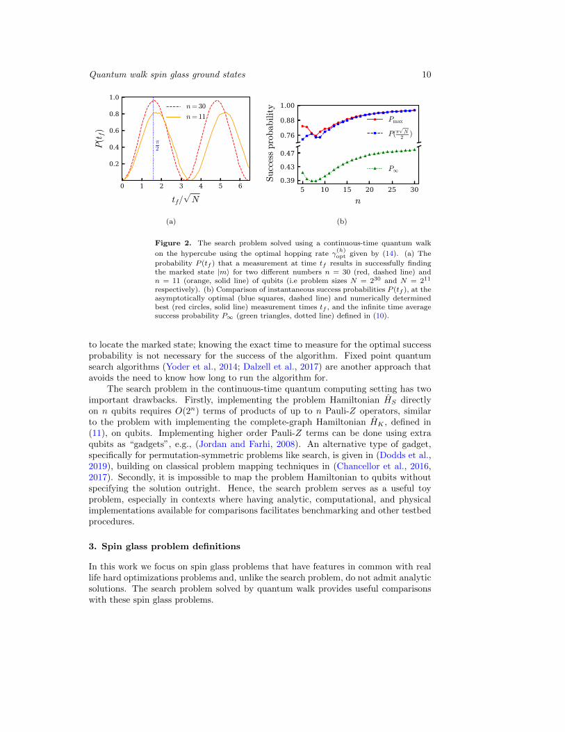
The variation of P (tf ) with tf is shown in figure 2(a) for search on hypercubegraphs of size N = 230 (i.e., n = 30 qubits) and N = 211 (i.e., n = 11 qubits), using

the optimal hopping rate γ(h)opt. The sinusoidal oscillations of the probability P (tf )

occur because the quantum walk is performing Rabi oscillations between the initialstate and the marked state. The two lowest energy levels of the full Hamiltonian H(γ)

with varying γ undergo an avoided level crossing at γ(h)opt and the associated eigenstates∣∣∣E0(γ

(h)opt

⟩) and

∣∣∣E1(γ(h)opt

⟩) are approximately the orthogonal equal superpositions of

the starting state and marked state,∣∣∣E0,1(γ

(h)opt

⟩) ' (|ψ(0)〉 ± |m〉)/2 1

2 . The gap

E1(γ(h)opt)−E0(γ

(h)opt) scales with the problem sizeN asO(N−1/2) (Childs and Goldstone,

2004).These simple, two-level dynamics describe the quantum walk solution to the

search problem well for large problem size N : the oscillations in the N = 230 casehave no visible irregularities. For smaller sizes, finite-size effects due to populationof higher energy levels are apparent: the oscillations in the N = 211 case have lowerprobability peaks and show some irregular behaviour, such as the small dip on the firstpeak. These finite-size effects are further illustrated in figure 2(b), which shows theinstantaneous success probability P (tf ) at the asymptotically optimal and numericallydetermined best times, as well as the infinite-time average success probability P∞defined in (10). All three probabilities show a pronounced dip around n = 8 qubits,with smooth behaviour only settling in for n > 12 qubits. Figure 2(b) also shows thatthe infinite-time probability P∞ asymptotes to a half. Hence, a quantum walk searchwith a random measurement time should on average only need to be repeated twice


0 1 2 3 4 5 6

tf/√N

0.2

0.4

0.6

0.8

1.0P(tf)

π2

n= 30

n= 11

(a)

0.76

0.88

1.00

Pmax

P(π√N

2)

5 10 15 20 25 30n

0.39

0.43

0.47

Succ

ess

pro

bability

P∞

(b)

Figure 2. The search problem solved using a continuous-time quantum walk

on the hypercube using the optimal hopping rate γ(h)opt given by (14). (a) The

probability P (tf ) that a measurement at time tf results in successfully findingthe marked state |m〉 for two different numbers n = 30 (red, dashed line) andn = 11 (orange, solid line) of qubits (i.e problem sizes N = 230 and N = 211

respectively). (b) Comparison of instantaneous success probabilities P (tf ), at theasymptotically optimal (blue squares, dashed line) and numerically determinedbest (red circles, solid line) measurement times tf , and the infinite time averagesuccess probability P∞ (green triangles, dotted line) defined in (10).

to locate the marked state; knowing the exact time to measure for the optimal successprobability is not necessary for the success of the algorithm. Fixed point quantumsearch algorithms (Yoder et al., 2014; Dalzell et al., 2017) are another approach thatavoids the need to know how long to run the algorithm for.

The search problem in the continuous-time quantum computing setting has twoimportant drawbacks. Firstly, implementing the problem Hamiltonian HS directlyon n qubits requires O(2n) terms of products of up to n Pauli-Z operators, similarto the problem with implementing the complete-graph Hamiltonian HK , defined in(11), on qubits. Implementing higher order Pauli-Z terms can be done using extraqubits as “gadgets”, e.g., (Jordan and Farhi, 2008). An alternative type of gadget,specifically for permutation-symmetric problems like search, is given in (Dodds et al.,2019), building on classical problem mapping techniques in (Chancellor et al., 2016,2017). Secondly, it is impossible to map the problem Hamiltonian to qubits withoutspecifying the solution outright. Hence, the search problem serves as a useful toyproblem, especially in contexts where having analytic, computational, and physicalimplementations available for comparisons facilitates benchmarking and other testbedprocedures.

3. Spin glass problem definitions

In this work we focus on spin glass problems that have features in common with reallife hard optimizations problems and, unlike the search problem, do not admit analyticsolutions. The search problem solved by quantum walk provides useful comparisonswith these spin glass problems.


3.1. Sherrington-Kirkpatrick spin glass

The Sherrington-Kirkpatrick (SK) spin glass Hamiltonian HSK (Sherrington andKirkpatrick, 1975) is defined on n spins as

HSK = −1

2

n−1∑(j 6=k)=0

JjkSjSk (15)

where Sj are the classical spins (Sj ∈ {−1, 1}) and the couplings Jjk are drawnindependently from the normal distribution N (µ, σ2

SK) with mean µ and variance σ2SK.

Finding the ground state of this Hamiltonian is NP-hard (Choi, 2010), and uniformlyhard, due to its finite-temperature phase transition (Sherrington and Kirkpatrick,1975).

It is computationally convenient to break the spin inversion symmetry by addingsingle-body field terms of the form

∑n−1j=0 hjSk, where hj are the field strength values.

Like the couplings Jjk, the fields hj are also drawn independently from N (µ, σ2SK).

When the fields strengths hj are drawn from the same distribution as the couplingstrengths Jjk, the hardness of finding the ground state follows directly from thehardness of the hj = 0 case. The SK spin glass with such fields is mathematicallyequivalent to a zero field spin glass with one more spin which is “fixed” in oneorientation. This is not true in general for different distributions of field strength hj .There are known examples in which fields can destroy spin glass behaviour (see, e.g.,Young and Katzgraber, 2004; Feng et al., 2014). In particular, if the field strengthsare much larger than the coupling strengths (|hj | � |Jjk| for all j, k), then the energyis minimized trivially when all the spins each minimize the energy with respect totheir individual fields. While the distribution of field strengths could be used to tunethe problem hardness, we do not use it in this way here, and only consider cases wherethe field and coupling strengths are drawn from the same distribution.

An astute reader will notice that if one effectively un-fixes the spin whichcorresponds to the fields (thus making all states two fold degenerate and convertingthe system to a double cover of the orignal system), these couplings will effectively beon average stronger by a factor of

√2. As this increase in coupling strength does not

scale with the number of spins, it is going to become less and less significant as thesize of the system is scaled up the hardness will be preserved.

The mapping into the quantum Ising model is almost trivial: the classical spinvariables Sj are simply mapped to Pauli-Z operators. Thus, the problem Hamiltonian

HSK becomes

HSK = −1

2

n−1∑(j 6=k)=0

JjkZjZk −n−1∑j=0

hjZj , (16)

The SK problem Hamiltonian differs from the search problem by having structure,produced by the ZjZk terms. As a result, the covariances between the energies of twobasis states depends on the Hamming-distance between them (Baldwin and Laumann,2018). Knowing the energy of one state gives some information about the energy ofstates that differ by a small number of bit-flips. This results in a distribution of theeigenenergies that is almost normal (as can be seen by plotting the distributions andnumerically calculating moments), but which deviates from normal in the tails of thedistribution.


3.2. Random energy model

To isolate the effect of the correlations in the SK problem, we compare it with therandom energy model (REM) (Derrida, 1980), in which the eigenenergies themselvesare independently drawn from a normal distribution. The problem Hamiltonian HREM

for REM is

HREM =

N−1∑j=0

Fj |j〉〈j| , (17)

with {|j〉}N−1j=0 the computational (Z) basis and the energies Fj drawn independently

from the normal distribution N (0, σ2REM).

REM has a similar energy level distribution to that of SK, apart from the tails.By definition it lacks the correlations: knowing the energy of one state gives noinformation about the energies of other states. Comparison between these two modelshighlights the effect of the pairwise structure in the SK model.

4. Numerical methods

The main tool used for the investigations in this work is numerical simulation. We arestudying computationally hard problems for which there are no tractable analyticalsolutions except in special cases.

For each number of qubits 5 ≤ n ≤ 20 we generated 10,000 random instances ofthe SK spin glass Hamiltonian, defined in (16), with the couplings Jjk and fields hjdrawn with a standard deviation σSK = ωSK, where ωSK is an arbitrary energy unit.The value ωSK = 5 was used for computational convenience. We also generated 10,000random instances of the REM Hamiltonian, defined in (17), for each number of qubits5 ≤ n ≤ 15, with normally-distributed energies Fj drawn with a standard deviationσREM = ωREM. The value ωREM = 1 was used for computational convenience. Notethat choosing any arbitrary constant for ω will only affect overall time and energyscales by a constant factor, and the energy unit ωSK has been scaled out of the plotswhere relevant.

The key quantity to determine numerically is the probability that the groundstate is found by running a quantum walk computation on each spin glass instance. Itis particularly convenient to compute the infinite-time probability P∞ given by (20),for sizes where full diagonalization is possible. Writing the spectral expansion of thefull computational quantum walk Hamiltonian as

H(γ) =

N−1∑a=0

Ea(γ) |Ea(γ)〉〈Ea(γ)| , (18)

with indices ordered such that Ea(γ) ≤ Ea+1(γ) and |Ea(γ)〉 the eigenstate witheigenvalue Ea(γ), we can write the instantaneous probability in terms of the spectralexpansions as

P (t) =∣∣∣⟨E(P )

0

∣∣∣ exp (−itH(γ)) |ψ(0)〉∣∣∣2

=

∣∣∣∣∣N−1∑a=0

exp (−itEa)⟨E

(P )0

∣∣∣Ea(γ)⟩〈Ea(γ)|ψ(0)〉

∣∣∣∣∣2


=

N−1∑a=0

∣∣∣⟨E(P )0

∣∣∣Ea(γ)⟩∣∣∣2 |〈Ea(γ)|ψ(0)〉|2 (19)

+

N−1∑a 6=b=0

[exp (−it(Ea − Eb))

⟨E

(P )0

∣∣∣Ea(γ)⟩×

〈Ea(γ)|ψ(0)〉⟨Eb(γ)

∣∣∣E(P )0

⟩〈ψ(0)|Eb(γ)〉

].

Assuming no degeneracy (that is, all gaps Ea −Eb are nonzero), which is justified forthe randomized nature of the SK and REM problems, the oscillatory terms cancel inthe infinite limit (because

∫∞0

dt exp (−itθ) = 0 for nonzero θ) to leave the infinite-timeaverage probability P∞ given by

P∞ =

N−1∑a=0

∣∣∣⟨E(P )0

∣∣∣Ea(γ)⟩∣∣∣2 |〈Ea(γ)|ψ(0)〉|2 . (20)

All of the numerical simulation in this work has been performed using the Python3language (Van Rossum and Drake, 2003), aided extensively by the IPython (Perez andGranger, 2007) interpreter and the Jupyter Notebook (Kluyver et al., 2016) system.The numerical heavy-lifting has been done using NumPy (Oliphant, 2006), SciPy(Jones et al., 2001–), and pandas (McKinney, 2010), and the plotting has been doneusing matplotlib (Hunter, 2007). The dynamical simulations have been performed bycomputing the action of the propagator exp (−itH(γ)) on the initial state |ψ(0)〉, usingthe sparse matrix functions within SciPy when possible. For the more computationallydemanding analyses, we were limited to n ≤ 11 by the computational resourcesavailable. Where relevant, figures in this paper have error bars included. However, inmost cases the error bars are much smaller than the size of the marker symbols usedand so are not visible. This is due to the size of the data sets (10k instances per valueof n), which provides a good level of accuracy for the average quantities.

Simulations were run on the Imperial and Durham University high performancecomputing facilities. The data for all the instances used is available on a permanentdata archive (Chancellor et al., 2019).

5. Quantum walks with spin glasses

In order to implement a quantum walk algorithm for finding the ground states ofthe spin glasses defined in section 3, we follow the procedure described in section2.2: Choose a quantum walk graph G and associated Hamiltonian HG, and addthe spin glass Hamiltonian to get the full computational quantum walk HamiltonianH(γ) = HG + HP , where HP refers to HSK or HREM as appropriate. Since thehypercube is the natural choice of graph for qubit implementations, we use this graph,with quantum walk Hamiltonian Hh defined in (12), unless otherwise indicated. Forthe initial state |ψ(0)〉, we use the equal superposition (7), which is the ground stateof the hypercube Hamiltonian Hh.

5.1. Setting the hopping rate

In contrast to the search problem, for SK and REM it is impossible to efficiently

calculate the optimal hopping rate γ(h)opt that maximizes the success probability.


0 1 2 3 4

γ/ωSK

0.01

0.03

0.05

P∞

∆γ(h)opt/ωSK

0.0 0.2 0.4 0.6 0.8

γ/ωREM

0.05

0.17

0.29

∆γ(h)opt/ωREM

Figure 3. Infinite-time success probability P∞ against hopping rate γ scaled bythe energy unit ωP for 3 typical 11-qubit examples of SK (left) and REM (right).

Also indicated (for one example in each plot) is the width ∆γ(h)opt of the peak (also

scaled by ωP ).

It is not even clear which measure of success probability should be maximizedbecause, unlike the search problem, there will be no efficient way to find the

optimal measurement time t(opt)f for any choice of hopping rate γ. To bootstrap the

investigation, we choose to define the optimal hopping-rate γ(h)opt with respect to one

of the average probabilities defined in (9); in particular, we choose the hopping ratethat maximizes the infinite-time average probability P∞ defined in (10). We makethis choice because the infinite-time average probability P∞ is numerically convenientto calculate, and because it has been seen to be a relevant measure of probability inthe search example, see figure 2(b). We will see in Subsection 5.3 that the probabilityP∞ typically agrees well with probabilities averaged over shorter and more practicaltime windows.

Some plots of the infinite-time probability P∞ against hopping rate γ for typical11-qubit examples of the SK and REM are shown in figure 3. Note that the maximalsuccess probability varies by an order of magnitude between the two problem-types,

with REM highest and SK lowest. While the optimal hopping rate γ(h)opt is instance-

dependent, these plots show that the dependence of infinite-time probability P∞ onhopping rate γ is typically characterised by broad, bumpy peaks for SK, and by narrow,well-defined peaks for REM. This implies that a precise value of the hopping rate γ isneeded for REM, while there is some tolerance to non-optimal values of the hoppingrate γ for SK for the sizes that we have studied.

To investigate the success probability more systematically, we performed a brute-

force numerical search to find the optimal hopping rate γ(h)opt that maximizes the success

probability P∞ for each spin glass instance from the data sets of 10k random instancesfor 5 ≤ n ≤ 11. This gives a baseline maximum average single run success probabilityfor the quantum walk algorithm.

The optimal hopping rates γ(h)opt correspond to the best a quantum walk algorithm

on the hypercube can possibly do in a single run. For practical algorithms, we needa heuristic method for choosing the hopping rate that can be calculated from theknown parameters. For the quantum walk search algorithm, the optimal hopping ratebalances the energy between the two components of the Hamiltonian, HP and HG.


0.5 1.0 1.5 2.0 2.5 3.0 3.5

γ(h)opt/ωP

02468

10p(γ

(h)

opt/ωP) γ

(h)heur/ωSK for SK

γ(h)heur/ωREM for REM

SK

REM

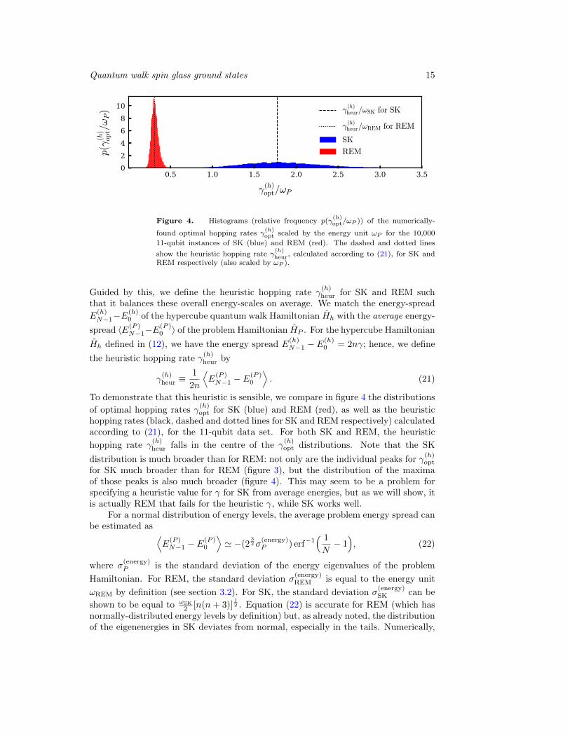
Figure 4. Histograms (relative frequency p(γ(h)opt/ωP )) of the numerically-

found optimal hopping rates γ(h)opt scaled by the energy unit ωP for the 10,000

11-qubit instances of SK (blue) and REM (red). The dashed and dotted lines

show the heuristic hopping rate γ(h)heur, calculated according to (21), for SK and

REM respectively (also scaled by ωP ).

Guided by this, we define the heuristic hopping rate γ(h)heur for SK and REM such

that it balances these overall energy-scales on average. We match the energy-spread

E(h)N−1−E

(h)0 of the hypercube quantum walk Hamiltonian Hh with the average energy-

spread 〈E(P )N−1−E

(P )0 〉 of the problem Hamiltonian HP . For the hypercube Hamiltonian

Hh defined in (12), we have the energy spread E(h)N−1 − E

(h)0 = 2nγ; hence, we define

the heuristic hopping rate γ(h)heur by

γ(h)heur ≡

1

2n

⟨E

(P )N−1 − E

(P )0

⟩. (21)

To demonstrate that this heuristic is sensible, we compare in figure 4 the distributions

of optimal hopping rates γ(h)opt for SK (blue) and REM (red), as well as the heuristic

hopping rates (black, dashed and dotted lines for SK and REM respectively) calculatedaccording to (21), for the 11-qubit data set. For both SK and REM, the heuristic

hopping rate γ(h)heur falls in the centre of the γ

(h)opt distributions. Note that the SK

distribution is much broader than for REM: not only are the individual peaks for γ(h)opt

for SK much broader than for REM (figure 3), but the distribution of the maximaof those peaks is also much broader (figure 4). This may seem to be a problem forspecifying a heuristic value for γ for SK from average energies, but as we will show, itis actually REM that fails for the heuristic γ, while SK works well.

For a normal distribution of energy levels, the average problem energy spread canbe estimated as ⟨

E(P )N−1 − E

(P )0

⟩' −(2

32σ

(energy)P ) erf−1

( 1

N− 1), (22)

where σ(energy)P is the standard deviation of the energy eigenvalues of the problem

Hamiltonian. For REM, the standard deviation σ(energy)REM is equal to the energy unit

ωREM by definition (see section 3.2). For SK, the standard deviation σ(energy)SK can be

shown to be equal to ωSK

2 [n(n+ 3)]12 . Equation (22) is accurate for REM (which has

normally-distributed energy levels by definition) but, as already noted, the distributionof the eigenenergies in SK deviates from normal, especially in the tails. Numerically,


we find that there is a multiplicative constant factor of approximately 0.887 thatcorrects the formula in (22) for SK for the effects of the non-normal tails. For thenumerical analysis, we use the numerically calculated average energy-spread at eachnumber of qubits n.

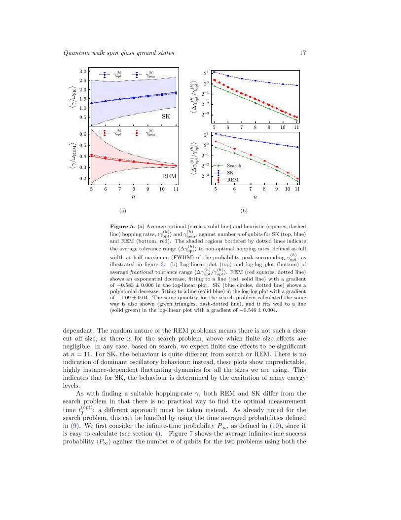
Figure 5(a) compares the heuristic hopping rate γ(h)heur and average optimal

hopping rate 〈γ(h)opt〉 at different numbers of qubits 5 ≤ n ≤ 11. The full width

at half maximum (FWHM) has also been calculated for each instance, to estimate

the tolerance ∆γ(h)opt to deviations from the optimal hopping rate γ

(h)opt (illustrated in

figure 3). The width of the shaded regions in figure 5(a) corresponds to the average

tolerance range 〈∆γ(h)opt〉 at each number n of qubits. While the heuristic hopping

rate differs slightly from the the average optimal hopping rate for SK, the average

tolerance range 〈∆γ(h)opt〉 is much broader, and does not shrink with increasing number

of qubits n. For REM, however, while we see close agreement on average, the tolerancerange shrinks quickly with the number of qubits n as the peaks (as in figure 3, right)

become narrower. This means that the heuristic hopping rate γ(h)heur is more likely to

lie further than 2∆γ(h)opt outside of the actual probability peak for each instance, even

though it agrees well with the average optimal hopping rate 〈γ(h)opt〉. Consequently, a

quantum walk with the heuristic hopping rate γ(h)heur does not perform well for most

REM instances.It is instructive to quantify this sensitivity to deviations from the optimal hopping

rate γ(h)opt. Figure 5(b) shows log-linear and log-log plots of the average fractional

tolerance range 〈∆γ(h)opt/γ

(h)opt〉 against number n of qubits for SK (blue circles), REM

(red squares) and search (green triangles) on the hypercube. For SK, the fractional

tolerance range 〈∆γ(h)opt/γ

(h)opt〉 decreases as approximately 1/n, while for REM and

search the decrease is approximately N−0.5. This decrease is expected theoreticallyfor search (Childs and Goldstone, 2004). The fitted lines do not show exactly a square-root dependence (exponent of −0.5) due to the finite size effects for small numbers ofqubits n ≤ 12.

Thus, we see that REM behaves like the search problem in a quantum walk

setting. For a precisely optimal hopping rate γ(h)opt, the success probability is high, but

this instance-dependent hopping rate is hard to predict, unlike for the analyticallytractable quantum walk search algorithm. Without this precise hopping rate, quantumwalks perform no better than guessing for the search problem and for REM. Incontrast, quantum walks applied to SK give a better-than-guessing success probability

P∞ > 1/N for the heuristic hopping rate γ(h)heur calculated according to (21).

With the conditions under which we can achieve a better-than-guessing successprobability characterised for the three problem types, SK, REM, and search, we turnto the scaling of this success probability with problem size N .

5.2. Success probability

Figure 6 shows how the single-time success probability P (tf ) varies with themeasurement time tf for two typical 11-qubit examples of SK and REM. In the REMcase, the behaviour is similar to that shown in figure 2(a) for search: an oscillatorynature indicating the dominance of a two-level avoided-crossing feature, but withevidence of the population of other energy-levels that lead to finite-size effects insearch. For REM, these finite-size effects are more pronounced, and are instance-


5 6 7 8 9 10 11n

0.5

1.0

1.5

2.0

2.5

3.0⟨ γ/ω

SK

⟩

SK

γ(h)opt γ

(h)heur

5 6 7 8 9 10 11n

0.2

0.3

0.4

0.5

0.6

⟨ γ/ωR

EM

⟩

REM

γ(h)opt γ

(h)heur

(a)

5 6 7 8 9 10 11

n

2−3

2−2

2−1

20

21

⟨ ∆γ

(h)

opt/γ

(h)

opt⟩

5 6 7 8 9 10 11

n

2−3

2−2

2−1

20

21

⟨ ∆γ

(h)

opt/γ

(h)

opt⟩

Search

SK

REM

(b)

Figure 5. (a) Average optimal (circles, solid line) and heuristic (squares, dashed

line) hopping rates, 〈γ(h)opt〉 and γ(h)heur, against number n of qubits for SK (top, blue)

and REM (bottom, red). The shaded regions bordered by dotted lines indicate

the average tolerance range 〈∆γ(h)opt〉 to non-optimal hopping rates, defined as full

width at half maximum (FWHM) of the probability peak surrounding γ(h)opt, as

illustrated in figure 3. (b) Log-linear plot (top) and log-log plot (bottom) of

average fractional tolerance range 〈∆γ(h)opt/γ(h)opt〉. REM (red squares, dotted line)

shows an exponential decrease, fitting to a line (red, solid line) with a gradientof −0.583 ± 0.006 in the log-linear plot. SK (blue circles, dotted line) shows apolynomial decrease, fitting to a line (solid blue) in the log-log plot with a gradientof −1.09 ± 0.04. The same quantity for the search problem calculated the sameway is also shown (green triangles, dash-dotted line), and it fits well to a line(solid green) in the log-linear plot with a gradient of −0.546± 0.004.

dependent. The random nature of the REM problems means there is not such a clearcut off size, as there is for the search problem, above which finite size effects arenegligible. In any case, based on search, we expect finite size effects to be significantat n = 11. For SK, the behaviour is quite different from search or REM. There is noindication of dominant oscillatory behaviour; instead, these plots show unpredictable,highly instance-dependent fluctuating dynamics for all the sizes we are using. Thisindicates that for SK, the behaviour is determined by the excitation of many energylevels.

As with finding a suitable hopping-rate γ, both REM and SK differ from thesearch problem in that there is no practical way to find the optimal measurement

time t(opt)f ; a different approach must be taken instead. As already noted for the

search problem, this can be handled by using the time averaged probabilities definedin (9). We first consider the infinite-time probability P∞, as defined in (10), since itis easy to calculate (see section 4). Figure 7 shows the average infinite-time successprobability 〈P∞〉 against the number n of qubits for the two problems using both the


0.02

0.06

0.10P(tf)

0 15 30 45 60ωSKtf

0.050.100.150.20

P(tf)

(a)

0.0

0.1

0.2

0.3

P(tf)

0 25 50 75 100 125 150 175 200ωREMtf

0.0

0.3

0.5

P(tf)

(b)

Figure 6. Instantaneous success probability P (tf ) against dimensionlessmeasurement time ωP tf for quantum walk on 2 typical 11-qubit SK examples

(a) and for 2 typical 11-qubit REM examples (b), using γ(h)opt.

5 6 7 8 9 10 11 12 13n

2−2

2−3

2−4

2−5

2−6

⟨ P ∞⟩

SK

γ(h)opt γ

(h)heur

5 6 7 8 9 10 11n

0.25

0.15

0.1 REM

γ(h)opt γ

(h)heur

Figure 7. Blue, left: Log-linear plot of average infinite time success probability〈P∞〉 against number of qubits n for SK, using optimal (circles, dotted line)

and heuristic (squares, dashed line) hopping rates γ(h)opt and γ

(h)heur. The data fit

log2〈P∞〉 = (−0.402 ± 0.001)n + (−0.174 ± 0.008) and log2〈P∞〉 = (−0.417 ±0.002)n + (−0.32 ± 0.01) respectively. Red, right: Log-linear plot of the samequantities for REM. In this case, the probability stays at constant order for theoptimal rate and decays for the heuristic rate.

optimal γ(h)opt and heuristic γ

(h)heur hopping rates. For SK, this gives exponential decay

with the number of qubits n in both cases: the average probability 〈P∞〉 changes withn according to

〈P∞〉 =O(N−0.402±0.001) with γ

(h)opt

O(N−0.417±0.002) with γ(h)heur

, (23)

where O may neglect factors logarithmic in its argument. That is, using the heuristic

hopping rate γ(h)heur instead of the optimal hopping rate γ

(h)opt has only a minor impact

on the average success probability 〈P∞〉.


For REM, the behaviour is quite different. With the optimal hopping rate γ(h)opt

we see a success probability P∞ of constant order but with a pronounced dip. Thisbehaviour is similar to that seen for the search problem, where the dip seen in figure2(b) is a finite-size effect. This similarity is expected, given the similarity betweenthe dynamical behaviour shown in figure 2(a) for search and in figure 6(b) for REM.

With the heuristic hopping rate γ(h)heur for REM, we see a significantly reduced success

probability P∞ compared to the optimal case. That is, the heuristic is performingpoorly, despite the good agreement shown in figure 5(a).

The clear difference in behaviour between SK and REM can be explained by the

different tolerances ∆γ(h)opt to deviations from the optimal hopping rate γ

(h)opt shown

in figure 5(a) and figure 5(b). For SK, the tolerance range is broad enough for the

heuristic to lie within it, while for REM the heuristic hopping rate γ(h)heur almost always

misses this range entirely even though it is close to the average optimal hopping rate⟨γ

(h)opt

⟩.

5.3. Mixing times

We have thus numerically determined an average success probability scaling withproblem size of ∼ O(N−0.42) for a quantum walk finding SK spin glass ground states,

using the heuristic hopping rate γ(h)heur. This is based on the infinite time-success

probability P∞, i.e., uniform sampling from the distribution of all possible run times.We now investigate the time dependence in more detail: can we sample from a finiterun time and still obtain the same speed up? Since P (0) = 1/N corresponds to randomguessing, there must be a minimum time before which it is not effective to measure.

We define a mixing-time τ(ε)mix to be the latest time, t, for which the time averaged

probabilities P (0, t) and P (0, 2t) at the two times t and 2t differ by a fraction greaterthan the fluctuation parameter ε,

τ(ε)mix = max{t :

∣∣∣ P (0, t)− P (0, 2t)

P (0, t)

∣∣∣ > ε}. (24)

This definition of τ(ε)mix is based on similar definitions found in prior work (Aharonov

et al., 2001), with modifications for computational convenience. We numerically

estimated the mixing-time τ(0.05)mix for each SK instance up to n = 11 qubits, using

the optimal hopping rate γ(h)opt for each instance. We simulated the quantum walk

computation dynamics for a successively-doubling duration until a time at which thecondition is met was reached. The fluctuation parameter ε = 0.05 corresponds to a

deviation of 5%. To verify that the mixing-time τ(0.05)mix correctly captures the relevant

dynamical timescale, we also numerically estimated it for the search problem at eachsystem size from n = 5 to n = 30 qubits. The search problem using continuous-timequantum walks can be mapped to the symmetric subspace, allowing larger sizes to

be analysed. The mixing-time τ(0.05)mix for search exhibits the expected exponential

timescale: the solid green line of best fit in figure 8(a) has the expected scaling with

problem size N of τ(0.05)mix = O(N1/2).

For search, the scaling is dominated by the run time, the success probability isO(1). However, this behaviour only emerges clearly above n ∼ 20. Below this, thebehaviour is influenced by the finite-size effects that arise due to population of higherenergy levels. This means it is not useful to analyse the behaviour of the REM time


5 10 15 20 25 30n

26

210

214

218τ(0

.05)

mix

Search

(a)

5 6 7 8 9 10 11

n

24.0

24.2

24.4

24.6

24.8

⟨ τ(0.0

5)m

ixω

SK

⟩

(b)

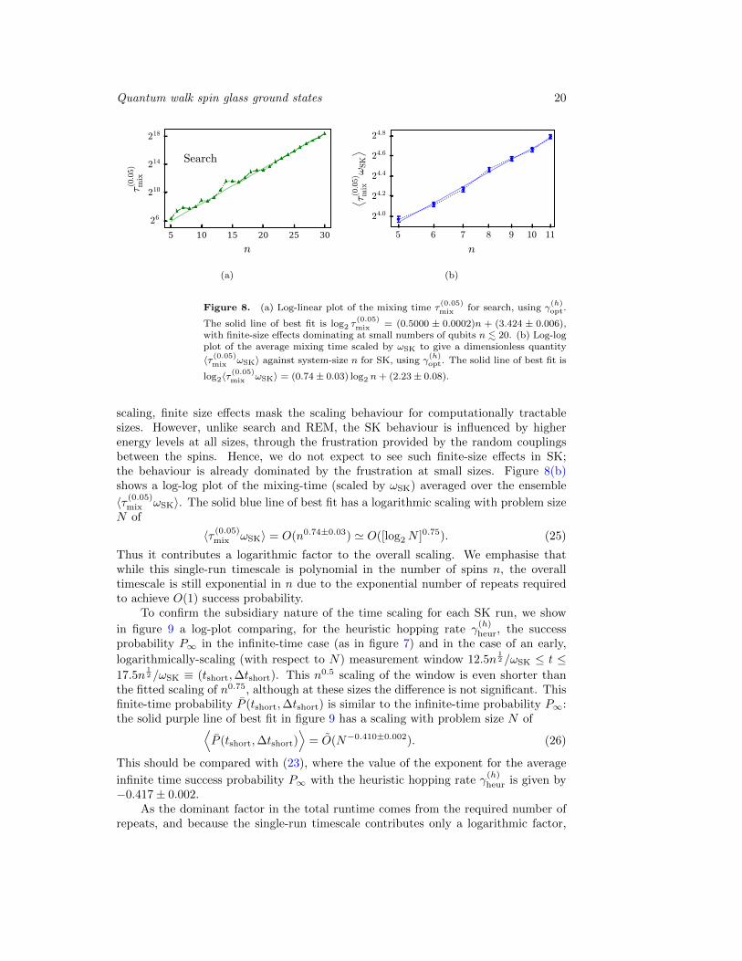
Figure 8. (a) Log-linear plot of the mixing time τ(0.05)mix for search, using γ

(h)opt.

The solid line of best fit is log2 τ(0.05)mix = (0.5000 ± 0.0002)n + (3.424 ± 0.006),

with finite-size effects dominating at small numbers of qubits n . 20. (b) Log-logplot of the average mixing time scaled by ωSK to give a dimensionless quantity

〈τ (0.05)mix ωSK〉 against system-size n for SK, using γ(h)opt. The solid line of best fit is

log2〈τ(0.05)mix ωSK〉 = (0.74± 0.03) log2 n+ (2.23± 0.08).

scaling, finite size effects mask the scaling behaviour for computationally tractablesizes. However, unlike search and REM, the SK behaviour is influenced by higherenergy levels at all sizes, through the frustration provided by the random couplingsbetween the spins. Hence, we do not expect to see such finite-size effects in SK;the behaviour is already dominated by the frustration at small sizes. Figure 8(b)shows a log-log plot of the mixing-time (scaled by ωSK) averaged over the ensemble

〈τ (0.05)mix ωSK〉. The solid blue line of best fit has a logarithmic scaling with problem size

N of

〈τ (0.05)mix ωSK〉 = O(n0.74±0.03) ' O([log2N ]0.75). (25)

Thus it contributes a logarithmic factor to the overall scaling. We emphasise thatwhile this single-run timescale is polynomial in the number of spins n, the overalltimescale is still exponential in n due to the exponential number of repeats requiredto achieve O(1) success probability.

To confirm the subsidiary nature of the time scaling for each SK run, we show

in figure 9 a log-plot comparing, for the heuristic hopping rate γ(h)heur, the success

probability P∞ in the infinite-time case (as in figure 7) and in the case of an early,

logarithmically-scaling (with respect to N) measurement window 12.5n12 /ωSK ≤ t ≤

17.5n12 /ωSK ≡ (tshort,∆tshort). This n0.5 scaling of the window is even shorter than

the fitted scaling of n0.75, although at these sizes the difference is not significant. Thisfinite-time probability P (tshort,∆tshort) is similar to the infinite-time probability P∞:the solid purple line of best fit in figure 9 has a scaling with problem size N of⟨

P (tshort,∆tshort)⟩

= O(N−0.410±0.002). (26)

This should be compared with (23), where the value of the exponent for the average

infinite time success probability P∞ with the heuristic hopping rate γ(h)heur is given by

−0.417± 0.002.As the dominant factor in the total runtime comes from the required number of

repeats, and because the single-run timescale contributes only a logarithmic factor,


6 8 10 12 14 16 18 20n

2−8

2−6

2−4

2−2

⟨ P⟩P∞

P(12.5√n

ωSK, 5.0

√n

ωSK)

P(0) = 2−n√P(0) = 2−n/2

Figure 9. Log-plot of average success probability using γ(h)heur against number of

qubits for infinite-time (blue circles and dotted line) as in figure 7, and averaged

over the short time window 12.5n12 ≤ tωSK ≤ 17.5n

12 (purple crosses and dashed

line). The short time data are fit by log2〈P 〉 = (−0.410±0.002)n+(−0.37±0.02)(solid purple line). The 2−n probability when measuring at t = 0, equivalent torandomly guessing (solid black line), and its square-root 2−n/2 (dotted black line)are also shown for comparison.

these results constitute good numerical evidence for an average total runtime whichscales with problem size N as ∼ O(N0.41) for using quantum walks to find spin glassground states, over the range of N in our data sets. This scaling is a better than thebest possible (quadratic) speed up achievable for quantum walk search algorithms.Moreover, it comes without the requirement for exponential precision in setting thehopping rate that renders practical use of quantum walk searching difficult for largeproblems. We now present some insights into where the improvement over searchcomes from.

6. Computational mechanisms

6.1. Role of correlations in SK

To investigate whether the energy correlations with Hamming distance in SK playa significant role in the computational process of finding the ground state with aquantum walk, we performed three additional sets of numerical tests.

Firstly, we used the same SK instances but performed the quantum walk usinga complete graph Hamiltonian HK , defined in (11), instead of the hypercube graphHamiltonian Hh. This removes the correspondence of Hamming-distance betweenclassical states with the distance between those states on the graph – for the completegraph, every state is one unit (edge) away from every other state. In terms of theHamiltonian, the transverse Ising term is replaced by sums of products of up to n Pauli-X operators that flip up to n qubits at the same time, in all possible combinations.

For each SK instance up to n = 11, we estimated the optimal hopping rate γ(K)opt for

the complete graph, and then used it to calculate the infinite-time probability P∞.Secondly, we constructed ‘scrambled SK’ instances, denoted sSK, by randomizing


5 6 7 8 9 10 11n

2−5

2−4

2−3

2−2

⟨ P ∞⟩

SK hypercube

SK complete

sSK hypercube

REM hypercube

REMGC hypercube

Figure 10. Log-linear plot showing the dependence on number of qubits n ofthe average success probability P∞ for SK on hypercube (blue circles, thick solidline), REM on hypercube (red crosses, dash-dotted line), sSK on hypercube (greentriangles, dotted line), SK on complete-graph (orange squares, dashed line) andREMGC on hypercube (purple diamonds, thin solid line). The optimal hopping

rates γ(h)opt are used in all cases.

which state corresponds to which energy in the SK instances. In doing so, we arriveat Hamiltonians with identical energy spectra to the SK instances, but without thecorrelations between energy difference and Hamming distance on the hypercube graph.This approach has similarities with previous work (Farhi et al., 2008, 2011; Hen, 2014).

For each sSK instance, we estimated the optimal hopping rate γ(h)opt, which is different

from that used for the ordinary SK versions. This hopping rate was then used tocalculate P∞.

Thirdly, we sorted the eigenenergies of each REM instance in increasing size andassigned them to the computational basis states in the order of a binary-reflectedGray code on their bitstrings, to arrive at a problem denoted REMGC. In doing so,we added some amount of Hamming-distance structure by ensuring that the closestenergies are assigned to states that differ by only a single bit-flip. For each REMGC

instance, we estimated an optimal hopping rate γ(h)opt, which is different from that used

for the ordinary REM problem. This was used to calculate the infinite-time probabilityP∞. While REMGC is not a hard problem as defined, it provides a useful example tocompare with how the quantum walk finds the ground state of a SK spin glass.

These three variants provide separate tests of the influence of the graph structure(choice of quantum walk Hamiltonian) and problem structure (pairwise correlationsin SK). Figure 10 shows how the infinite-time probability P∞ varies with the numberof qubits n for these three variants, alongside SK and REM on a hypercube graphfrom figure 7. The variation of P∞ with the number of qubits n for the five variantsis clearly split into two groups, behaviour like REM and search on the one hand, andbehaviour like SK on the other. Removing the correlations from SK by scramblingthe energies (sSK) results in behaviour like REM and search. Moreover, removing thecorrespondence between distance and Hamming weight by using the complete graphinstead of the hypercube also changes the SK problem behaviour to be like REM and


search. In the opposite direction, inserting pairwise correlations into REM via a Graycode (REMGC) results in problems that are much more like SK than like the REMproblems on a hypercube graph.

From this, we infer that the problem structure – in this case the pairwisecorrelations in SK – needs to be matched by a compatible driver Hamiltonian – in thiscase the hypercube/transverse Ising – to obtain better than quadratic scaling. Thistype of local structure in the solution space is exploited in many classical algorithms.For example, classical Monte Carlo optimizations that use a single bit flip update ruleare naturally using this hypercube structure. Using a complete graph instead wouldcorrespond to flipping a random number of bits, which is equivalent to guessing ateach step.

6.2. Energy conservation dynamics

Continuous-time quantum walk time evolution is unitary, and there is no timedependence in the Hamiltonian that can lead to energy gain or loss by the system.Hence, it is important to consider how it can find a lower energy state than it startsin (with respect to HP ) with any better-than-guessing probability. For the searchproblem, this happens through an analog of Rabi flopping (see figure 2), cyclingbetween the initial and solution states. However, the dominant avoided level crossingstructure is not present in the spin glasses to provide this mechanism.

We now show that there is a very generic mechanism (also describedindependently by Hastings (2019)) that relies on starting in the ground state of thequantum walk part of Hamiltonian HG. Let 〈O〉ψ(t) for operator O be defined by

〈ψ(t)|O|ψ(t)〉 = 〈O〉ψ(t). Then, by linearity, and the definition of H(γ) in (8), theenergy expectation at time t is

〈H(γ)〉ψ(t) = 〈HG〉ψ(t) + 〈HP 〉ψ(t). (27)

Due to the unitarity of the evolution under a time-independent Hamiltonian, thisexpectation energy will not change over time, giving

〈H(γ)〉ψ(t) = 〈H(γ)〉ψ(0). (28)

which yields

〈HG〉ψ(t) − 〈HG〉ψ(0) = 〈HP 〉ψ(0) − 〈HP 〉ψ(t). (29)

As |ψ(0)〉 is chosen to be the ground state of HG, the LHS must be non-negative.Furthermore, as |ψ(0)〉 is not an eigenstate of H(γ), some dynamics are guaranteed tooccur and so the LHS must become positive at early times. Therefore, the RHS mustalso be non-negative always and positive at early times. Thus, taking any final timetf , we get the inequality

1

tf

tf∫t=0

dt〈HP 〉ψ(t) < 〈HP 〉ψ(0). (30)

Equation (30) shows that performing time evolution under the computationalquantum walk Hamiltonian from the initial state |ψ(0)〉 is guaranteed to lower theenergy of the system with respect to HP (the expectation value 〈HP 〉ψ(t)). This

implies that the overlap with low energy eigenstates of HP will increase, at least forshort times. A measurement in the computational basis will thus be on average morelikely than a random guess to produce a low energy state.


Starting in a low energy state is thus important for the success of the quantumwalk algorithm (we have checked this numerically). It also implies that encoding priorinformation into the initial state will help, provided this is given in the form of a lowerenergy state than the uniform superposition state. This could be the final state froma previous run, for example, which will be explored further in Nita et al. (2020). It isalso necessary to bias the quantum walk Hamiltonian so that its ground state matchesthis biased initial state. Since this starting state is a known computational basis state,it is possible to do this biasing for suitably designed hardware.

For many optimization problem applications, it is helpful to find a low energystate, even if it is not actually the true ground state. From this point of view, thatquantum walks necessarily lower the expectation energy with respect to the problemHamiltonian is very appealing as a computational mechanism. This argument by itselfdoes not provide a guaranteed scaling or quantum speed up, but it does explain howthe quantum walk dynamics work in this setting, where there is no way to lose (orgain) energy. It is possible to generalise these arguments beyond time-independentHamiltonians (Callison et al., 2020b), to include monotonic functions A(t) and B(t)in (4).

To illustrate this energy redistribution mechanism, the plots in figure 11 show howthe expectation value 〈HG〉ψ(t) of the quantum walk Hamiltonian (green solid-line)

and the expectation value 〈HP 〉ψ(t) of the problem Hamiltonian (red solid-line) varyduring a quantum walk. We have included the instantaneous success probability P (t)(faint grey) to show that the timescale used is long enough for significant dynamicsto take place. A typical 10-qubit SK example is shown in figure 11(a) and a typical10-qubit REM example is shown in figure 11(b), both on the hypercube using their

respective optimal hopping rates γ(h)opt. Also shown is the ground state eigenvalue

〈HP 〉E(P )0

of the problem Hamiltonian (red, dash-dotted line) and the ground state

eigenvalue 〈HG〉ψ(0) of the quantum walk Hamiltonian (green, dashed line). In both

SK and REM, the initial evolution takes the state away from the HG ground state,raising the HG expectation value, and thereby lowering the HP expectation value toa point around which it fluctuates for the duration simulated. This clearly showsthe energy redistribution mechanism at work, and the short time scale over which itappears.

7. Summary and outlook

In this work, we have shown numerically that continuous-time quantum walks are aviable computational method for finding ground states of hard spin glass problems.We have produced strong numerical evidence for a better-than-search polynomialquantum speed up over random guessing, with a scaling of the average single runsuccess probability ∼ O(N−0.41), using data sets of size 5 ≤ n ≤ 20 spins (32 ≤N ≤ 1, 048, 576). Moreover, and importantly, this is obtained without the need to setparameters exponentially precisely, as is required for quantum walk search algorithms.The hopping rate γ, that determines the relative strengths of the quantum walk andproblem Hamiltonians, can be estimated from the overall energy scales, which aredetermined by the hardware and encoding of the problem.

To explain why quantum walks are able to do better than quantum searching inthis case, we compared variants on the spin glass problems that remove or add pairwisecorrelations, and compared the hypercube graph quantum walk Hamiltonian with


0 4 8 1215

10

5

0

5

10

E/ω

SK

0.025

0.050

0.075

0.100

P(t

)

SK

⟨HG

⟩ψ(t)⟨

HP

⟩ψ(t)

⟨HP

⟩E

(P)0⟨

HG

⟩ψ(0)

(a)

0 50 100 150

2

1

0

1

2

E/ω

RE

M

0.1

0.2

0.3

0.4

0.5

P(t

)

REM

⟨HG

⟩ψ(t)⟨

HP

⟩ψ(t)

⟨HP

⟩E

(P)0⟨

HG

⟩ψ(0)

(b)

Figure 11. The expectation value 〈HG〉ψ(t) of the quantum walk Hamiltonian

(green, thin solid line) and the expectation value 〈HP 〉ψ(t) of the problemHamiltonian (red, thick solid line) for a typical 10 qubit (a) SK and (b) REMinstance. The ground state energy eigenvalues of the quantum walk Hamiltonian(green, dashed line) and problem Hamiltonians (red, dash-dotted line) are alsoshown. To illustrate that significant dynamics take place over the timescales used,the instantaneous probabilities P (t) are also shown (grey, faint line). The energyvalues are on the left axes, while probability values are on the right axes.

the complete graph quantum walk Hamiltonian. This showed that the combinationof pairwise correlations in the encoding of the problem and a matching single spinflip quantum walk Hamiltonian is required to exploit the correlations. The singlespin-flips driven by the transverse field terms Xj in the hypercube quantum walk

Hamiltonian are the correct operators for the pairwise interaction terms ZjZk in thespin glass Hamiltonian. A single spin flip on either qubit j or k changes the energyfor that term from high to low, or vice versa. Since we can choose how to encode theproblems into the Hamiltonians, and there are known methods to convert higher orderterms to pairwise terms (Bremner et al., 2002; Dattani, 2019), we can arrange to usethis mechanism both for its computational advantages and practicality for hardwareimplementation as the transverse Ising Hamiltonian.

To explain how quantum walks are able to find low energy states when the closedquantum dynamics have no mechanism for losing energy, we showed how starting in theground state of the quantum walk part of the Hamiltonian guarantees dynamics thatdecrease the expectation value of the energy with respect to the problem Hamiltonian.This also ensures that prior information can be provided by starting in lower energystates, from which improved solutions can be found. Exploiting this process willallow an optimal quantum algorithm to be built from multiple quantum walk runsthat use the information gained from prior runs. Performing multiple quantum walkruns in early, noisy quantum hardware is a more viable approach than maintainingcoherence for sufficiently accurate adiabatic algorithms. Quantum walks may also besimpler to implement since they do not require time dependent controls. This workthus provides a significant advance in understanding how to exploit quantum walks inpractical hardware for optimization problems.

It is likely that further insights into the computational effectiveness of quantumwalks in this transverse Ising Hamiltonian setting are to be found in current knowledge

REFERENCES 26

of spin glass phases in the presence of transverse fields. The spin glass transitionitself is not fully understood, in neither the quantum nor classical case (see, e.g.,Parisi, 1980; Fisher and Huse, 1987, 1988; Thirumalai et al., 1989; Larson et al., 2013;Young, 2017; Magalhaes et al., 2017). However, the phases of interest for computationare not the spin glass phases themselves, but the phases where transitions betweenstates are still occurring at a rapid enough rate to find solution states. Extremelylong equilibration timescales are a defining property of all glass phases, including spinglasses (Bouchaud et al., 1998; Cugliandolo, 2002). Since the equilibration (mixing)

times τ(ε)mix we find in section 5.3 for the SK spin glass only scale polynomially with the

number of spins, it is most likely that at the optimal hopping rates γ(h)opt, our quantum

walks are not in a finite size precursor to a spin glass phase, but rather in a precursor toa paramagnetic phase, for which equilibration times can be fast. Given that the systemshould localize more in lower energy states for smaller transverse fields, it is reasonable

that our optimal hopping rates γ(h)opt occur near the edge of the precursor to the spin

glass phase. Furthermore, the mild scaling of the width ∆γ(h)opt of the peak around the

optimal hopping rate γ(h)opt suggests that the regime where quantum walks performs

well may correspond to the second paramagnetic phase observed in Magalhaes et al.(2017). Polynomial gaps have been found around the spin glass–paramagnetic phasetransition in a related model in (Knysh, 2016).

A numerical study such as this inevitably leaves open questions regarding theasymptotic scaling of the problems. In particular, we observed a range of hardnessin the SK data sets and future work will investigate what fraction of the instancesare actually hard for classical algorithms. Forthcoming work applying similartechniques to Max2SAT (Callison et al., 2020a) will characterise the hardness ofsmall random instances in more detail, and establish quantum walks as an effectivetool for hard optimization problems more generally. While general methods areknown to speed up the best classical algorithms (Hartwig et al., 1984) for thistype of problem (Montanaro, 2018, 2019), further work is required to determinewhether an optimal continuous-time quantum walk algorithm can be devised thatfully leverages the advantage from the correlations. Nonetheless, our work represents asignificant advance in developing continuous-time quantum walk computation for hardoptimization problems, and provides key insights into the computational mechanismsthat can be exploited over short timescales, well-suited to the limited coherence timesof noisy, intermediate scale quantum hardware.

Acknowledgments

VK and NC funded by UK EPSRC fellowship EP/L022303/1 and NC funded byEPSRC grant EP/S00114X/1. AC funded by EPSRC grant EP/L016524/1 via theImperial College London CDT in Controlled Quantum Dynamics. We thank Prof. IfanG. Hughes and Dr Ashley Montanaro for helpful discussions.

References

Dorit Aharonov, Andris Ambainis, Julia Kempe, and Umesh Vazirani. Quantum walkson graphs. In Proceedings of the Thirty-third Annual ACM Symposium on Theoryof Computing, STOC ’01, pages 50–59, New York, NY, USA, 2001. ACM. ISBN

REFERENCES 27

1-58113-349-9. doi: 10.1145/380752.380758. URL http://doi.acm.org/10.1145/

380752.380758.

Andris Ambainis, Kaspars Balodis, Janis Iraids, Martins Kokainis, Krisjanis Prusis,and Jevgenijs Vihrovs. Quantum Speedups for Exponential-Time DynamicProgramming Algorithms, pages 1783–1793. Assoc. for Comp. Machinery, NewYork, 2019. doi: 10.1137/1.9781611975482.107. URL https://epubs.siam.org/

doi/abs/10.1137/1.9781611975482.107.

Mohammad H. Amin, Evgeny Andriyash, Jason Rolfe, Bohdan Kulchytskyy, andRoger Melko. Quantum Boltzmann machine. Phys. Rev. X, 8:021050, May 2018.doi: 10.1103/PhysRevX.8.021050. URL https://link.aps.org/doi/10.1103/

PhysRevX.8.021050.

C. L. Baldwin and C. R. Laumann. Quantum algorithm for energy matching in hardoptimization problems. Phys. Rev. B, 97:224201, Jun 2018. doi: 10.1103/PhysRevB.97.224201. URL https://link.aps.org/doi/10.1103/PhysRevB.97.224201.

Rene Beier and Berthold Vocking. Random knapsack in expected polynomialtime. Journal of Computer and System Sciences, 69(3):306 – 329, 2004. ISSN0022-0000. doi: https://doi.org/10.1016/j.jcss.2004.04.004. URL http://www.

sciencedirect.com/science/article/pii/S0022000004000431. Special Issue onSTOC 2003.

C. Bennett, E. Bernstein, G. Brassard, and U. Vazirani. Strengths andWeaknesses of Quantum Computing. SIAM Journal on Computing, 26(5):1510–1523, 1997. doi: 10.1137/S0097539796300933. URL https://doi.org/10.1137/

S0097539796300933.

Hannes Bernien, Sylvain Schwartz, Alexander Keesling, Harry Levine, Ahmed Omran,Hannes Pichler, Soonwon Choi, Alexander S. Zibrov, Manuel Endres, MarkusGreiner, Vladan Vuletic, and Mikhail D. Lukin. Probing many-body dynamicson a 51-atom quantum simulator. Nature, 551:579 EP –, 11 2017. URL https:

//doi.org/10.1038/nature24622.

Zhengbing Bian, Fabian Chudak, William G. Macready, Lane Clark, and FrankGaitan. Experimental Determination of Ramsey Numbers. Phys. Rev. Lett., 111:130505, Sep 2013. doi: 10.1103/PhysRevLett.111.130505. URL https://link.

aps.org/doi/10.1103/PhysRevLett.111.130505.

Sergio Boixo, Tameem Albash, Federico M. Spedalieri, Nicholas Chancellor, andDaniel A. Lidar. Experimental signature of programmable quantum annealing.Nature Communications, 4:2067 EP –, 06 2013. URL https://doi.org/10.1038/

ncomms3067.

Jean-Philippe Bouchaud, Leticia F Cugliandolo, Jorge Kurchan, and Marc Mezard.Out of equilibrium dynamics in spin-glasses and other glassy systems, pages 161–223. World Scientific, Singapore, 1998. doi: 10.1142/9789812819437 0006. URLhttps://www.worldscientific.com/doi/abs/10.1142/9789812819437_0006.

Michael J. Bremner, Christopher M. Dawson, Jennifer L. Dodd, Alexei Gilchrist,Aram W. Harrow, Duncan Mortimer, Michael A. Nielsen, and Tobias J. Osborne.Practical Scheme for Quantum Computation with Any Two-Qubit Entangling Gate.Phys. Rev. Lett., 89:247902, Nov 2002. doi: 10.1103/PhysRevLett.89.247902. URLhttps://link.aps.org/doi/10.1103/PhysRevLett.89.247902.

http://doi.acm.org/10.1145/380752.380758

http://doi.acm.org/10.1145/380752.380758

https://epubs.siam.org/doi/abs/10.1137/1.9781611975482.107

https://epubs.siam.org/doi/abs/10.1137/1.9781611975482.107

https://link.aps.org/doi/10.1103/PhysRevX.8.021050


https://link.aps.org/doi/10.1103/PhysRevB.97.224201

http://www.sciencedirect.com/science/article/pii/S0022000004000431

http://www.sciencedirect.com/science/article/pii/S0022000004000431

https://doi.org/10.1137/S0097539796300933

https://doi.org/10.1137/S0097539796300933

https://doi.org/10.1038/nature24622


https://link.aps.org/doi/10.1103/PhysRevLett.111.130505


https://doi.org/10.1038/ncomms3067


https://www.worldscientific.com/doi/abs/10.1142/9789812819437_0006


REFERENCES 28

Adam Callison, Max Festenstein, Lewis Light, Nicholas Chancellor, and Viv Kendon.Hybrid adiabatic-quantum-walk algorithms applied to Max2SAT, in preparation.,2020a. in preparation.

Adam Callison, Viv Kendon, and Nicholas Chancellor. Tools for practical quantumannealing, 2020b. in preparation.

N. Chancellor, S. Zohren, P. A. Warburton, S. C. Benjamin, and S. Roberts. A directmapping of Max k-SAT and high order parity checks to a chimera graph. ScientificReports, 6:37107 EP –, 11 2016. URL https://doi.org/10.1038/srep37107.

N Chancellor, A Callison, V Kendon, and F Mintert. Finding spin-glass groundstates using quantum walks [dataset], 2019. URL https://doi.org/10.15128/

r21544bp097. Data archive at Durham University, UK, for spin glass instancesused in this work.

Nicholas Chancellor. Modernizing quantum annealing using local searches. NewJournal of Physics, 19(2):023024, feb 2017. doi: 10.1088/1367-2630/aa59c4. URLhttps://doi.org/10.1088/1367-2630/aa59c4.

Nicholas Chancellor, Stefan Zohren, and Paul A. Warburton. Circuit designfor multi-body interactions in superconducting quantum annealing systems withapplications to a scalable architecture. npj Quantum Information, 3(21), 2017.doi: 10.1038/s41534-017-0022-6. URL https://www.nature.com/articles/

s41534-017-0022-6.

Andrew M. Childs and Jeffrey Goldstone. Spatial search by quantum walk. Phys.Rev. A, 70:022314, Aug 2004. doi: 10.1103/PhysRevA.70.022314. URL https:

//link.aps.org/doi/10.1103/PhysRevA.70.022314.

Andrew M. Childs, Richard Cleve, Enrico Deotto, Edward Farhi, Sam Gutmann, andDaniel A. Spielman. Exponential Algorithmic Speedup by a Quantum Walk. InProceedings of the Thirty-fifth Annual ACM Symposium on Theory of Computing,STOC ’03, pages 59–68, New York, NY, USA, 2003. ACM. ISBN 1-58113-674-9. doi:10.1145/780542.780552. URL http://doi.acm.org/10.1145/780542.780552.

Vicky Choi. Adiabatic quantum algorithms for the NP-complete Maximum-WeightIndependent set, Exact Cover and 3SAT problems, 2010. URL https://arxiv.

org/abs/1004.2226. arXiv:1004.2226.

G. E. Coxson, C. R. Hill, and J. C. Russo. Adiabatic quantum computing for findinglow-peak-sidelobe codes. In 2014 IEEE High Performance Extreme ComputingConference (HPEC), pages 1–6, Sep. 2014. doi: 10.1109/HPEC.2014.7040953. URLhttps://ieeexplore.ieee.org/abstract/document/7040953.

Leticia F Cugliandolo. Dynamics of glassy systems, 2002. URL https://arxiv.org/

abs/cond-mat/0210312. arXiv preprint cond-mat/0210312.

D-Wave. D-Wave Systems Inc. website, 1999–. URL http://www.dwavesys.com/.[Online; accessed Tuesday 24th December, 2019].

Alexander M. Dalzell, Theodore J. Yoder, and Isaac L. Chuang. Fixed-point adiabaticquantum search. Phys. Rev. A, 95:012311, Jan 2017. doi: 10.1103/PhysRevA.95.012311. URL https://link.aps.org/doi/10.1103/PhysRevA.95.012311.

Nike Dattani. Quadratization in discrete optimization and quantum mechanics, 2019.URL http://arxiv.org/abs/1901.04405. arXiv:1901.04405.

Gemma De las Cuevas and Toby S. Cubitt. Simple universal models capture allclassical spin physics. Science, 351(6278):1180–1183, 2016. ISSN 0036-8075. doi:

https://doi.org/10.1038/srep37107

https://doi.org/10.15128/r21544bp097

https://doi.org/10.15128/r21544bp097

https://doi.org/10.1088/1367-2630/aa59c4

https://www.nature.com/articles/s41534-017-0022-6

https://www.nature.com/articles/s41534-017-0022-6

https://link.aps.org/doi/10.1103/PhysRevA.70.022314


http://doi.acm.org/10.1145/780542.780552

https://arxiv.org/abs/1004.2226


https://ieeexplore.ieee.org/abstract/document/7040953

https://arxiv.org/abs/cond-mat/0210312

https://arxiv.org/abs/cond-mat/0210312

http://www.dwavesys.com/


http://arxiv.org/abs/1901.04405

REFERENCES 29

10.1126/science.aab3326. URL http://science.sciencemag.org/content/351/

6278/1180.

B. Derrida. Random-Energy Model: Limit of a Family of Disordered Models.Phys. Rev. Lett., 45:79–82, Jul 1980. doi: 10.1103/PhysRevLett.45.79. URLhttps://link.aps.org/doi/10.1103/PhysRevLett.45.79.

A. Ben Dodds, Viv Kendon, Charles S. Adams, and Nicholas Chancellor. Practicaldesigns for permutation-symmetric problem hamiltonians on hypercubes, Sep 2019.URL https://link.aps.org/doi/10.1103/PhysRevA.100.032320.

Qian-Heng Duan, Shuo Zhang, Wei Wu, and Ping-Xing Chen. An alternative approachto construct the initial hamiltonian of the adiabatic quantum computation. ChinesePhysics Letters, 30(1):010302, Jan 2013. doi: 10.1088/0256-307x/30/1/010302.URL https://doi.org/10.1088/0256-307x/30/1/010302.

Edward Farhi and Sam Gutmann. Quantum computation and decision trees. Phys.Rev. A, 58:915–928, Aug 1998. doi: 10.1103/PhysRevA.58.915. URL http:


Edward Farhi, Jeffrey Goldstone, Sam Gutmann, and Michael Sipser. Quantumcomputation by adiabatic evolution, 2000. URL https://arxiv.org/abs/

quant-ph/0001106. arXiv preprint quant-ph/0001106.

Edward Farhi, Jeffrey Goldstone, Sam Gutmann, Joshua Lapan, Andrew Lundgren,and Daniel Preda. A Quantum Adiabatic Evolution Algorithm Applied to RandomInstances of an NP-Complete Problem. Science, 292(5516):472–475, 2001. ISSN0036-8075. doi: 10.1126/science.1057726. URL http://science.sciencemag.org/

content/292/5516/472.

Edward Farhi, Jeffrey Goldstone, Sam Gutmann, and Daniel Nagaj. How to make thequantum adiabatic algorithm fail. International Journal of Quantum Information,06(03):503–516, 2008. doi: 10.1142/S021974990800358X. URL https://doi.org/

10.1142/S021974990800358X.

Edward Farhi, Jeffrey Goldstone, David Gosset, Sam Gutmann, and Peter Shor.Unstructured randomness, small gaps and localization. Quantum Information &Computation, 11(9-10):840–854, Sep 2011. URL http://www.rintonpress.com/

xxqic11/qic-11-910/0840-0854.pdf.

Edward Farhi, Jeffrey Goldstone, and Sam Gutmann. A quantum approximateoptimization algorithm, 2014a. URL https://arxiv.org/abs/1411.4028.arXiv:1411.4028.

Edward Farhi, Jeffrey Goldstone, and Sam Gutmann. A quantum approximateoptimization algorithm applied to a bounded occurrence constraint problem, 2014b.URL https://arxiv.org/abs/1412.6062. arXiv:1412.6062.

Sheng Feng, Ye Fang, Ka-Ming Tam, Zhifeng Yun, J Ramanujam, Juana Moreno,and Mark Jarrell. Three Dimensional Edwards-Anderson Spin Glass Model in anExternal Field, 2014. URL https://arxiv.org/abs/1403.4560. arXiv:1403.4560.

A.B. Finnila, M.A. Gomez, C. Sebenik, C. Stenson, and J.D. Doll. Quantumannealing: A new method for minimizing multidimensional functions. ChemicalPhysics Letters, 219(5):343 – 348, 1994. ISSN 0009-2614. doi: https://doi.org/10.1016/0009-2614(94)00117-0. URL http://www.sciencedirect.com/science/

article/pii/0009261494001170.

http://science.sciencemag.org/content/351/6278/1180




https://doi.org/10.1088/0256-307x/30/1/010302

http://link.aps.org/doi/10.1103/PhysRevA.58.915

http://link.aps.org/doi/10.1103/PhysRevA.58.915

https://arxiv.org/abs/quant-ph/0001106

https://arxiv.org/abs/quant-ph/0001106



https://doi.org/10.1142/S021974990800358X

https://doi.org/10.1142/S021974990800358X

http://www.rintonpress.com/xxqic11/qic-11-910/0840-0854.pdf

http://www.rintonpress.com/xxqic11/qic-11-910/0840-0854.pdf




http://www.sciencedirect.com/science/article/pii/0009261494001170


REFERENCES 30

D S Fisher and D A Huse. Absence of many states in realistic spin glasses. Journal ofPhysics A: Mathematical and General, 20(15):L1005–L1010, oct 1987. doi: 10.1088/0305-4470/20/15/013. URL https://doi.org/10.1088/0305-4470/20/15/013.

Daniel S. Fisher and David A. Huse. Equilibrium behavior of the spin-glass orderedphase. Phys. Rev. B, 38:386–411, Jul 1988. doi: 10.1103/PhysRevB.38.386. URLhttps://link.aps.org/doi/10.1103/PhysRevB.38.386.

Tobias Graß. Quantum annealing with longitudinal bias fields. Phys. Rev. Lett., 123:120501, Sep 2019. doi: 10.1103/PhysRevLett.123.120501. URL https://link.

aps.org/doi/10.1103/PhysRevLett.123.120501.

Tobias Graß and Maciej Lewenstein. Hybrid annealing: Coupling a quantum simulatorto a classical computer. Phys. Rev. A, 95:052309, May 2017. doi: 10.1103/PhysRevA.95.052309. URL https://link.aps.org/doi/10.1103/PhysRevA.95.

052309.

Lov K. Grover. A fast quantum mechanical algorithm for database search. InProceedings of the Twenty-eighth Annual ACM Symposium on Theory of Computing,STOC ’96, pages 212–219, New York, NY, USA, 1996. ACM. ISBN 0-89791-785-5. doi: 10.1145/237814.237866. URL http://doi.acm.org/10.1145/237814.

237866.

Stuart Hadfield, Zhihui Wang, Bryan O’Gorman, Eleanor G. Rieffel, Davide Venturelli,and Rupak Biswas. From the quantum approximate optimization algorithm to aquantum alternating operator ansatz. Algorithms, 12(2), 2019. ISSN 1999-4893.doi: 10.3390/a12020034. URL http://www.mdpi.com/1999-4893/12/2/34.

Firas Hamze, Jack Raymond, Christopher A. Pattison, Katja Biswas, and Helmut G.Katzgraber. The wishart planted ensemble: A tunably-rugged pairwise ising modelwith a first-order phase transition, 2019. URL https://arxiv.org/abs/1906.

00275. arXiv preprint arXiv:1906.00275.

A. Hartwig, F. Daske, and S. Kobe. A recursive branch-and-bound algorithmfor the exact ground state of ising spin-glass models. Computer PhysicsCommunications, 32(2):133 – 138, 1984. ISSN 0010-4655. doi: https://doi.org/10.1016/0010-4655(84)90066-3. URL http://www.sciencedirect.com/science/

article/pii/0010465584900663.

Matthew B. Hastings. Duality in Quantum Quenches and Classical ApproximationAlgorithms: Pretty Good or Very Bad, November 2019. ISSN 2521-327X. URLhttps://doi.org/10.22331/q-2019-11-11-201.

Itay Hen. Continuous-time quantum algorithms for unstructured problems. Journalof Physics A: Mathematical and Theoretical, 47(4):045305, Jan 2014. doi: 10.1088/1751-8113/47/4/045305. URL https://doi.org/10.1088/1751-8113/47/

4/045305.

Itay Hen. Equation planting: A tool for benchmarking ising machines. Phys. Rev.Applied, 12:011003, Jul 2019. doi: 10.1103/PhysRevApplied.12.011003. URLhttps://link.aps.org/doi/10.1103/PhysRevApplied.12.011003.

John D Hunter. Matplotlib: A 2D graphics environment. Computing in science &engineering, 9(3):90, 2007.

Takahiro Inagaki, Yoshitaka Haribara, Koji Igarashi, Tomohiro Sonobe, ShuheiTamate, Toshimori Honjo, Alireza Marandi, Peter L. McMahon, Takeshi Umeki,Koji Enbutsu, Osamu Tadanaga, Hirokazu Takenouchi, Kazuyuki Aihara, Ken-ichi

https://doi.org/10.1088/0305-4470/20/15/013






http://doi.acm.org/10.1145/237814.237866

http://doi.acm.org/10.1145/237814.237866

http://www.mdpi.com/1999-4893/12/2/34





https://doi.org/10.22331/q-2019-11-11-201

https://doi.org/10.1088/1751-8113/47/4/045305

https://doi.org/10.1088/1751-8113/47/4/045305

https://link.aps.org/doi/10.1103/PhysRevApplied.12.011003

REFERENCES 31

Kawarabayashi, Kyo Inoue, Shoko Utsunomiya, and Hiroki Takesue. A coherentIsing machine for 2000-node optimization problems. Science, 354(6312):603–606,2016. ISSN 0036-8075. URL http://science.sciencemag.org/content/354/

6312/603.

M. W. Johnson, M. H. S. Amin, S. Gildert, T. Lanting, F. Hamze, N. Dickson,R. Harris, A. J. Berkley, J. Johansson, P. Bunyk, E. M. Chapple, C. Enderud,J. P. Hilton, K. Karimi, E. Ladizinsky, N. Ladizinsky, T. Oh, I. Perminov, C. Rich,M. C. Thom, E. Tolkacheva, C. J. S. Truncik, S. Uchaikin, J. Wang, B. Wilson, andG. Rose. Quantum annealing with manufactured spins. Nature, 473:194 EP –, 052011. URL https://doi.org/10.1038/nature10012.

Eric Jones, Travis Oliphant, Pearu Peterson, et al. SciPy: Open source scientific toolsfor Python, 2001–. URL http://www.scipy.org/. [Online; accessed Tuesday 24th

December, 2019].

Stephen Jordan and Edward Farhi. Perturbative gadgets at arbitrary orders. PhysicalReview A, 77, 02 2008. URL https://link.aps.org/doi/10.1103/PhysRevA.77.

062329.

Tadashi Kadowaki and Hidetoshi Nishimori. Quantum annealing in the transverseIsing model. Phys. Rev. E, 58:5355–5363, Nov 1998. doi: 10.1103/PhysRevE.58.5355. URL https://link.aps.org/doi/10.1103/PhysRevE.58.5355.

Helmut G. Katzgraber, Firas Hamze, and Ruben S. Andrist. Glassy chimeras couldbe blind to quantum speedup: Designing better benchmarks for quantum annealingmachines. Phys. Rev. X, 4:021008, Apr 2014. doi: 10.1103/PhysRevX.4.021008.URL https://link.aps.org/doi/10.1103/PhysRevX.4.021008.

Kostyantyn Kechedzhi, Vadim Smelyanskiy, Jarrod R. McClean, Vasil S. Denchev,Masoud Mohseni, Sergei Isakov, Sergio Boixo, Boris Altshuler, and Hartmut Neven.Efficient Population Transfer via Non-Ergodic Extended States in Quantum SpinGlass. In Stacey Jeffery, editor, 13th Conference on the Theory of QuantumComputation, Communication and Cryptography (TQC 2018), volume 111 ofLeibniz International Proceedings in Informatics (LIPIcs), pages 9:1–9:16, Dagstuhl,Germany, 2018. Schloss Dagstuhl–Leibniz-Zentrum fuer Informatik. ISBN 978-3-95977-080-4. doi: 10.4230/LIPIcs.TQC.2018.9. URL http://drops.dagstuhl.de/

opus/volltexte/2018/9256.

K Kim, S Korenblit, R Islam, E E Edwards, M-S Chang, C Noh, H Carmichael, G-D Lin, L-M Duan, C C Joseph Wang, J K Freericks, and C Monroe. Quantumsimulation of the transverse ising model with trapped ions. New Journal ofPhysics, 13(10):105003, oct 2011. doi: 10.1088/1367-2630/13/10/105003. URLhttps://doi.org/10.1088/1367-2630/13/10/105003.

Thomas Kluyver, Benjamin Ragan-Kelley, Fernando Perez, Brian Granger, MatthiasBussonnier, Jonathan Frederic, Kyle Kelley, Jessica Hamrick, Jason Grout, SylvainCorlay, Paul Ivanov, Damian Avila, Safia Abdalla, and Carol Willing. JupyterNotebooks – a publishing format for reproducible computational workflows. InF. Loizides and B. Schmidt, editors, Positioning and Power in Academic Publishing:Players, Agents and Agendas, pages 87 – 90. IOS Press, 2016.

Sergey Knysh. Zero-temperature quantum annealing bottlenecks in the spin-glassphase. Nature Communications, 7:12370 EP –, 08 2016. URL https://doi.org/

10.1038/ncomms12370.




http://www.scipy.org/



https://link.aps.org/doi/10.1103/PhysRevE.58.5355


http://drops.dagstuhl.de/opus/volltexte/2018/9256

http://drops.dagstuhl.de/opus/volltexte/2018/9256

https://doi.org/10.1088/1367-2630/13/10/105003



REFERENCES 32

Michael Krivelevich and Dan Vilenchik. Solving random satisfiable 3CNF formulas inexpected polynomial time. In Proceedings of the Seventeenth Annual ACM-SIAMSymposium on Discrete Algorithm, SODA ’06, pages 454–463, Philadelphia, PA,USA, 2006. Society for Industrial and Applied Mathematics. ISBN 0-89871-605-5.URL http://dl.acm.org/citation.cfm?id=1109557.1109608.

Derek Larson, Helmut G. Katzgraber, M. A. Moore, and A. P. Young. Spinglasses in a field: Three and four dimensions as seen from one space dimension.Phys. Rev. B, 87:024414, Jan 2013. doi: 10.1103/PhysRevB.87.024414. URLhttps://link.aps.org/doi/10.1103/PhysRevB.87.024414.

Zhaokai Li, Nikesh S Dattani, Xi Chen, Xiaomei Liu, Hengyan Wang, RichardTanburn, Hongwei Chen, Xinhua Peng, and Jiangfeng Du. High-fidelity adiabaticquantum computation using the intrinsic Hamiltonian of a spin system: Applicationto the experimental factorization of 291311, 2017. URL https://arxiv.org/abs/

1706.08061. arXiv preprint arXiv:1706.08061.

Andrew Lucas. Ising formulations of many NP problems. Frontiers in Physics, 2:5, 2014. ISSN 2296-424X. doi: 10.3389/fphy.2014.00005. URL https://www.

frontiersin.org/article/10.3389/fphy.2014.00005.

S. G. Magalhaes, C. V. Morais, F. M. Zimmer, M. J. Lazo, and F. D. Nobre. Nonlinearsusceptibility of a quantum spin glass under uniform transverse and randomlongitudinal magnetic fields. Phys. Rev. B, 95:064201, Feb 2017. doi: 10.1103/PhysRevB.95.064201. URL https://link.aps.org/doi/10.1103/PhysRevB.95.

064201.

S. Marsh and J. B. Wang. A quantum walk-assisted approximate algorithm forbounded NP optimisation problems. Quantum Information Processing, 18(3):61, Jan 2019. ISSN 1573-1332. doi: 10.1007/s11128-019-2171-3. URL https:

//doi.org/10.1007/s11128-019-2171-3.

Jeffrey Marshall, Davide Venturelli, Itay Hen, and Eleanor G. Rieffel. Power ofpausing: Advancing understanding of thermalization in experimental quantumannealers. Phys. Rev. Applied, 11:044083, Apr 2019. doi: 10.1103/PhysRevApplied.11.044083. URL https://link.aps.org/doi/10.1103/PhysRevApplied.11.

044083.

Michael Marzec. Portfolio Optimization: Applications in Quantum Computing,chapter 4, pages 73–106. John Wiley & Sons, Ltd, 2016. ISBN 9781118593486.doi: 10.1002/9781118593486.ch4. URL https://onlinelibrary.wiley.com/doi/

abs/10.1002/9781118593486.ch4.

Wes McKinney. Data structures for statistical computing in python. In Proceedings ofthe 9th Python in Science Conference, volume 445, pages 51–56. Austin, TX, 2010.

Peter L. McMahon, Alireza Marandi, Yoshitaka Haribara, Ryan Hamerly, CarstenLangrock, Shuhei Tamate, Takahiro Inagaki, Hiroki Takesue, Shoko Utsunomiya,Kazuyuki Aihara, Robert L. Byer, M. M. Fejer, Hideo Mabuchi, and YoshihisaYamamoto. A fully programmable 100-spin coherent Ising machine with all-to-all connections. Science, 354(6312):614–617, 2016. ISSN 0036-8075. doi:10.1126/science.aah5178. URL http://science.sciencemag.org/content/354/

6312/614.

Ashley Montanaro. Quantum-walk speedup of backtracking algorithms. Theoryof Computing, 14(15):1–24, 2018. doi: 10.4086/toc.2018.v014a015. URL http:

//www.theoryofcomputing.org/articles/v014a015. arXiv:1509.02374.

http://dl.acm.org/citation.cfm?id=1109557.1109608




https://www.frontiersin.org/article/10.3389/fphy.2014.00005

https://www.frontiersin.org/article/10.3389/fphy.2014.00005



https://doi.org/10.1007/s11128-019-2171-3

https://doi.org/10.1007/s11128-019-2171-3



https://onlinelibrary.wiley.com/doi/abs/10.1002/9781118593486.ch4

https://onlinelibrary.wiley.com/doi/abs/10.1002/9781118593486.ch4



http://www.theoryofcomputing.org/articles/v014a015

http://www.theoryofcomputing.org/articles/v014a015

REFERENCES 33

Ashley Montanaro. Quantum speedup of branch-and-bound algorithms, 2019.arXiv:1906.10375.

James G. Morley, Nicholas Chancellor, Sougato Bose, and Viv Kendon. Quantumsearch with hybrid adiabatic–quantum-walk algorithms and realistic noise. Phys.Rev. A, 99:022339, Feb 2019. doi: 10.1103/PhysRevA.99.022339. URL https:


Dominic J. Moylett, Noah Linden, and Ashley Montanaro. Quantum speedup of thetraveling-salesman problem for bounded-degree graphs. Phys. Rev. A, 95:032323,Mar 2017. doi: 10.1103/PhysRevA.95.032323. URL https://link.aps.org/doi/

10.1103/PhysRevA.95.032323.

Laur Nita, Matthew Walsh, Jie Chen, Adam Callison, Viv Kendon, and NicholasChancellor. Effectiveness of a general continuous time subroutine for hybridquantum/classical optimisation, 2020. in preparation.

Travis E Oliphant. A guide to NumPy, volume 1. Trelgol Publishing USA, 2006.

G Parisi. The order parameter for spin glasses: a function on the interval 0-1. Journalof Physics A: Mathematical and General, 13(3):1101–1112, mar 1980. doi: 10.1088/0305-4470/13/3/042. URL https://doi.org/10.1088/0305-4470/13/3/042.

G. Passarelli, V. Cataudella, and P. Lucignano. Improving quantum annealing of theferromagnetic p-spin model through pausing. Phys. Rev. B, 100:024302, Jul 2019.doi: 10.1103/PhysRevB.100.024302. URL https://link.aps.org/doi/10.1103/

PhysRevB.100.024302.

Alejandro Perdomo-Ortiz, Salvador E. Venegas-Andraca, and Alan Aspuru-Guzik.A study of heuristic guesses for adiabatic quantum computation. QuantumInformation Processing, 10(1):33–52, Feb 2011. ISSN 1573-1332. doi: 10.1007/s11128-010-0168-z. URL https://doi.org/10.1007/s11128-010-0168-z.

Alejandro Perdomo-Ortiz, Neil Dickson, Marshall Drew-Brook, Geordie Rose, andAlan Aspuru-Guzik. Finding low-energy conformations of lattice protein modelsby quantum annealing. Scientific Reports, 2:571 EP –, 08 2012. URL https:

//doi.org/10.1038/srep00571.

F. Perez and B. E. Granger. IPython: A System for Interactive Scientific Computing.Computing in Science Engineering, 9(3):21–29, May 2007. ISSN 1521-9615. doi:10.1109/MCSE.2007.53.

Neil Shenvi, Julia Kempe, and K. Birgitta Whaley. Quantum random-walk searchalgorithm. Phys. Rev. A, 67:052307, May 2003. doi: 10.1103/PhysRevA.67.052307.URL https://link.aps.org/doi/10.1103/PhysRevA.67.052307.

David Sherrington and Scott Kirkpatrick. Solvable model of a spin-glass. Phys.Rev. Lett., 35:1792–1796, Dec 1975. doi: 10.1103/PhysRevLett.35.1792. URLhttps://link.aps.org/doi/10.1103/PhysRevLett.35.1792.

D Thirumalai, Qiang Li, and T R Kirkpatrick. Infinite-range Ising spin glass in atransverse field. Journal of Physics A: Mathematical and General, 22(16):3339–3349, aug 1989. doi: 10.1088/0305-4470/22/16/023. URL https://doi.org/10.

1088/0305-4470/22/16/023.

Guido Van Rossum and Fred L Drake. Python language reference manual. NetworkTheory United Kingdom, 2003.

Theodore J. Yoder, Guang Hao Low, and Isaac L. Chuang. Fixed-point quantumsearch with an optimal number of queries. Phys. Rev. Lett., 113:210501, Nov





https://doi.org/10.1088/0305-4470/13/3/042



https://doi.org/10.1007/s11128-010-0168-z





https://doi.org/10.1088/0305-4470/22/16/023

https://doi.org/10.1088/0305-4470/22/16/023

REFERENCES 34

2014. doi: 10.1103/PhysRevLett.113.210501. URL https://link.aps.org/doi/

10.1103/PhysRevLett.113.210501.

A. P. Young. Stability of the quantum Sherrington-Kirkpatrick spin glass model.Phys. Rev. E, 96:032112, Sep 2017. doi: 10.1103/PhysRevE.96.032112. URLhttps://link.aps.org/doi/10.1103/PhysRevE.96.032112.

A. P. Young and Helmut G. Katzgraber. Absence of an Almeida-Thouless linein three-dimensional spin glasses. Phys. Rev. Lett., 93:207203, Nov 2004. doi:10.1103/PhysRevLett.93.207203. URL https://link.aps.org/doi/10.1103/

PhysRevLett.93.207203.

Leo Zhou, Sheng-Tao Wang, Soonwon Choi, Hannes Pichler, and Mikhail D. Lukin.Quantum approximate optimization algorithm: Performance, mechanism, andimplementation on near-term devices, 2018. URL https://arxiv.org/abs/1812.

01041. arXiv preprint arXiv:1812.01041.



https://link.aps.org/doi/10.1103/PhysRevE.96.032112





finding spin glass ground states using quantum walksfinding spin glass ground states using quantum...

Documents