finding ranges of optimal transcript expression ... · 12/13/2019 · tions, especially under the...

Finding ranges of optimal transcript expression quantification incases of non-identifiability

Cong Ma∗1, Hongyu Zheng∗1, and Carl Kingsford†1

1Computational Biology Department, School of Computer Science, Carnegie Mellon University,5000 Forbes Ave., Pittsburgh, PA

December 13, 2019

Abstract

Current expression quantification methods suffer from a fundamental but under-characterized typeof error: the most likely estimates for transcript abundances are not unique. Probabilistic models areat the core of current quantification methods. The scenario where a probabilistic model has multipleoptimal solutions is known as non-identifiability. In expression quantification, multiple configurationsof transcript expression may be equally likely to generate the sequencing reads and the underlying trueexpression cannot be uniquely determined. It is still unknown from existing methods what the set ofmultiple solutions is or how far the equally optimal solutions are from each other. Such information isnecessary for evaluating the reliability of analyses that are based on a single inferred expression vectorand for extending analyses to take all optimal solutions into account. We propose methods to computethe range of optimal estimates for the expression of each transcript when the probabilistic model forexpression inference is non-identifiable. The accuracy and identifiability of expression estimates dependon the completeness of input reference transcriptome, therefore our method also takes an assumed per-centage of expression from combinations of known junctions into consideration. Applying our methodon 16 Human Body Map samples and comparing with the single expression vector quantified by Salmon,we observe that the ranges of optimal abundances are on the same scale as Salmon’s estimate. Analyz-ing the overlap of ranges of optima in differential expression (DE) detection reveals that the majority ofpredictions are reliable, but there are a few unreliable predictions for which switching to other optimalabundances may lead to similar expression between DE conditions. The source code can be found athttps://github.com/Kingsford-Group/subgraphquant.

Keywords: expression quantification, alternative splicing, uncertainty, non-identifiability, differentialexpression.

1 Introduction

With the wide usage of gene or transcript expression data, we have seen improvement in probabilistic modelsof expression quantification [1–4], as well as characterization and evaluation of the errors of quantified ex-pression [5–7]. However, there is an under-characterized type of estimation error, due to the non-uniqueness∗Equal contribution†To whom correspondence should be addressed: [email protected]

1

.CC-BY 4.0 International license(which was not certified by peer review) is the author/funder. It is made available under aThe copyright holder for this preprintthis version posted December 13, 2019. . https://doi.org/10.1101/2019.12.13.875625doi: bioRxiv preprint

https://doi.org/10.1101/2019.12.13.875625

http://creativecommons.org/licenses/by/4.0/

of solutions to the probabilistic model. When multiple sets of expression of transcripts give rise to thesequencing library with equal probability, current methods only output one of the optimal solutions. It isusually unknown what the other optimal solutions are or how different they are from each other.

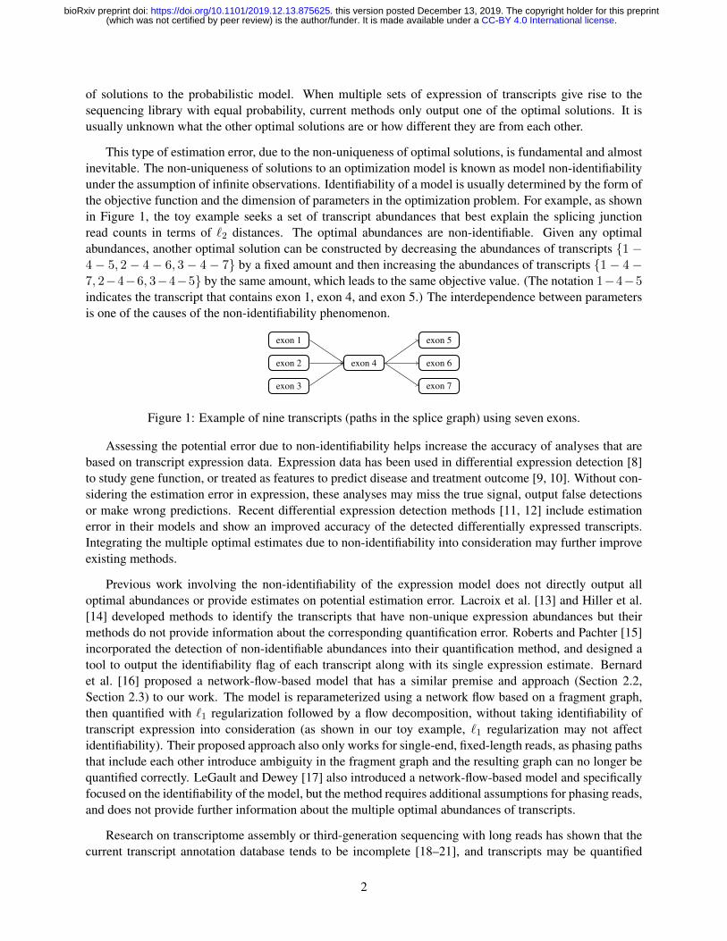
This type of estimation error, due to the non-uniqueness of optimal solutions, is fundamental and almostinevitable. The non-uniqueness of solutions to an optimization model is known as model non-identifiabilityunder the assumption of infinite observations. Identifiability of a model is usually determined by the form ofthe objective function and the dimension of parameters in the optimization problem. For example, as shownin Figure 1, the toy example seeks a set of transcript abundances that best explain the splicing junctionread counts in terms of `2 distances. The optimal abundances are non-identifiable. Given any optimalabundances, another optimal solution can be constructed by decreasing the abundances of transcripts {1 −4− 5, 2− 4− 6, 3− 4− 7} by a fixed amount and then increasing the abundances of transcripts {1− 4−7, 2−4−6, 3−4−5} by the same amount, which leads to the same objective value. (The notation 1−4−5indicates the transcript that contains exon 1, exon 4, and exon 5.) The interdependence between parametersis one of the causes of the non-identifiability phenomenon.

exon 1

exon 2

exon 3

exon 4 exon 6

exon 5

exon 7

Figure 1: Example of nine transcripts (paths in the splice graph) using seven exons.

Assessing the potential error due to non-identifiability helps increase the accuracy of analyses that arebased on transcript expression data. Expression data has been used in differential expression detection [8]to study gene function, or treated as features to predict disease and treatment outcome [9, 10]. Without con-sidering the estimation error in expression, these analyses may miss the true signal, output false detectionsor make wrong predictions. Recent differential expression detection methods [11, 12] include estimationerror in their models and show an improved accuracy of the detected differentially expressed transcripts.Integrating the multiple optimal estimates due to non-identifiability into consideration may further improveexisting methods.

Previous work involving the non-identifiability of the expression model does not directly output alloptimal abundances or provide estimates on potential estimation error. Lacroix et al. [13] and Hiller et al.[14] developed methods to identify the transcripts that have non-unique expression abundances but theirmethods do not provide information about the corresponding quantification error. Roberts and Pachter [15]incorporated the detection of non-identifiable abundances into their quantification method, and designed atool to output the identifiability flag of each transcript along with its single expression estimate. Bernardet al. [16] proposed a network-flow-based model that has a similar premise and approach (Section 2.2,Section 2.3) to our work. The model is reparameterized using a network flow based on a fragment graph,then quantified with `1 regularization followed by a flow decomposition, without taking identifiability oftranscript expression into consideration (as shown in our toy example, `1 regularization may not affectidentifiability). Their proposed approach also only works for single-end, fixed-length reads, as phasing pathsthat include each other introduce ambiguity in the fragment graph and the resulting graph can no longer bequantified correctly. LeGault and Dewey [17] also introduced a network-flow-based model and specificallyfocused on the identifiability of the model, but the method requires additional assumptions for phasing reads,and does not provide further information about the multiple optimal abundances of transcripts.

Research on transcriptome assembly or third-generation sequencing with long reads has shown that thecurrent transcript annotation database tends to be incomplete [18–21], and transcripts may be quantified

2


https://doi.org/10.1101/2019.12.13.875625


erroneously because the unannotated transcripts responsible for the reads are not present in the reference.Therefore, it is important to quantify all optimal abundances under various reference completeness assump-tions, especially under the incomplete reference assumption. Under such assumption, the parameter spaceincludes the expressions of novel transcripts and the dimension is expanded, making the parameters moresusceptible to non-identifiability.

In this work, we propose methods to construct the set of optimal estimates for transcript abundances un-der three assumptions about reference completeness given a probabilistic model. The current quantificationprobabilistic models are usually convex, thus the range of optima for each transcript is a closed interval. Weuse the phrase “range of optima” to refer to the set of optima projected to abundance of a single transcript.Assuming a complete reference, we propose a linear programming formulation to bound the range of optimalabundances for each transcript based on a phasing aware reparameterization of the model. Assuming thatthe reference transcriptomis incomplete but the splice graph is correct, we propose a set of max-flow-basedalgorithms on an adapted splice graph for reconstructing the set of optima. Finally, under the assumptionthat the reference is incomplete but a known, given percentage of expression is contributed by the reference,we derive the range of optima using an affine combination of the optima constructed in the previous twocases.

Using our method, we evaluate the distance between the single solution of the quantifier Salmon [4]to the other abundances in the range of optima on Human Body Map samples. We observe that most ofthe Salmon estimates are at the boundaries of the range, and the upper bounds of the range of optimalabundances tend to be within 10 fold of Salmon’s estimates.

Applying our method on sequencing samples of MCF10 cell line, we use the range of optimal expressionto evaluate the detected differentially expressed transcripts. Between the group of samples treated with andwithout epidermal growth factor (EGF), 257 transcripts are detected as differentially expressed based onthe single estimates. The majority are reliable after considering the ranges of optima when assuming thereference transcriptome is somewhat complete and contributes to more than 40% of the expression, whilethere are still a few unreliable detections for which the two groups’ ranges of optimal expression overlap.

2 Methods

2.1 Overview

Our goal is to calculate the range of optima for each transcript and to analyze the effect of non-identifiabilityon quantification. Our first step is to reparameterize the probabilistic model with a more identifiable param-eter set, called path abundances. Assuming all reads originate from known transcripts (complete reference),we calculate the range of optima by a linear-programming-based reallocation process from known quantifi-cation results. We cover the reparameterization and reallocation process in Section 2.2.

On the other end of the completeness spectrum, we have the assumption that reads may also be gener-ated from unannotated transcripts with existing splicing junctions but not present in reference transcriptome.Existing approaches are ill-suited for this setting, as the number of transcripts is too large to enumerate. Wesolve this problem in three steps. We describe how to derive the constraints governing the new set of param-eters by first modeling the matching of phasing paths to transcripts as a multiple pattern matching problem,then defining a network flow over the matching automaton (Section 2.3). We next develop efficient infer-ence algorithms for the resulting flow (Section 2.4) and calculate the range of optima via a new algorithmic

3


https://doi.org/10.1101/2019.12.13.875625


framework called subgraph quantification (Section 2.5).

In Section 2.6, we investigate the rest of the reference completeness spectrum by proposing a hy-brid model of read generation, and design a reliability check for differential expression calls against non-identifiability. Figure 2 provides an overview of different components of our methods.

Figure 2: Steps to derive range of optima under different reference completeness assumptions. Grey blocksindicate steps built upon existing methods.

2.2 Reparameterized Transcript Quantification

We start with the core model of transcript quantification at the foundation of most modern methods [1–4]. Assume the paired-end reads from some RNA-seq experiment are error-free and uniquely aligned toa reference genome with possible gaps. We denote the set of reads as F , the set of transcripts as T ={T1, T2, · · · , Tn}with corresponding length l1, l2, · · · , ln and abundance (copies of molecules) c1, c2, · · · , cn.The transcripts per million (TPM) values are calculated by normalizing {ci} and multiplying by 106. Underthe generative model, the probability of observing F is:

P (F | T , c) =∏f∈F

∑i∈A(f)

P (Ti)P (f | Ti)

A(f) is the set of transcripts onto which f can map. Let D(l) be the distribution of generated fragmentlength. With absence of bias correction, P (f | Ti) is proportional to D(f) = D(l(f)), where l(f) denotesthe fragment length inferred from mapping. Define the effective length for Ti as li =

∑lij=1

∑lik=j D(k −

j + 1) (which can be interpreted as the total probability for Ti to generate a fragment), and P (f | Ti) =D(f)/li. Probability of generating a fragment from Ti is assumed to be proportional to its abundance timesits effective length, meaning P (Ti) ∝ ci li. We discuss other definitions of effective length in Section S1.1and refer to previous papers [1–4, 22] for more detailed explanation of the model. This leads to:

P (F | T , c) =∏f∈F

(∑i∈A(f)

ci)D(f)/(∑Ti∈T

ci li)

We now propose an alternative view of the probabilistic model with paths on splice graphs in order toderive a compact parameter set for the quantification problem.

Splice graphs are succinct representations of alternative splicing events in a gene. A splice graph is adirected acyclic graph where each vertex represents a full or partial exon and each edge either connects twoadjacent partial exons or corresponds to a splicing junction. Two special vertices S and T represent startand end of transcripts instead of exons. We assume the splice graph is constructed so each transcript can beuniquely mapped to a S − T path p(Ti) on the graph, and the read library satisfies that each fragment f canbe uniquely mapped to a (non S − T ) path p(f) on the graph. With this setup, i ∈ A(f) if and only if p(f)is a subpath of p(Ti), or p(f) ⊂ p(Ti).

4


https://doi.org/10.1101/2019.12.13.875625


We now define cp =∑

i:Ti∈T ,p⊂p(Ti) ci to be the total abundance of transcripts including path p, called a

path abundance, and lp =∑lk

i=1

∑lkj=i 1(p(Tk[i, j]) = p)D(j− i+ 1) called path effective length, where

Tk[i, j] is the fragment generated from transcript k from base i to base j and 1(·) is the indicator function.Intuitively, the path effective length is the total probability of sampling a fragment that maps exactly to thegiven path. Next, let P be the set of paths from the splice graph satisfying lp > 0. We can re-calculate thenormalization term of the model by

∑Ti∈T ci li =

∑p∈P cp lp (proof in Section S1.2). The likelihood can

now be rewritten as follows:

P (F | T , c) =∏f∈F

(∑

j:p(f)⊂p(Tj)

cj)Df/(∑p∈P

cp lp) ∝∏f∈F

cp(f)/(∑p∈P

cp lp)

As shown here, we reparameterize the model with cp, the path abundance. When the transcriptome iscomplex, the dimension of cp is lower than the number of transcripts, a direct manifestation of the non-identifiability problem. In practice, we further reduce the size of P by discarding long paths with small lpand no mapped reads, as they contribute little to the likelihood function (See Section S1.3 for details). Ourmodel also enables certain bias corrections as described in Section S1.4.

With the reparameterized model, we now derive the range of optimal expression values for each tran-script assuming all reads are generated from known transcripts. The reference abundances {cRi } are derivedwith existing tools, such as Salmon or kallisto [3]. We assume {cRi } yields the optimal likelihood. If themodel is non-identifiable, it means there are other sets of transcript abundances {ci} that yield exactly thesame likelihood. As we have shown above, it suffices for {ci} to generate an identical set of path abundancesas {cRi } to be optimal. The set of transcript abundance that satisfies this condition and therefore indistin-guishable from cR is defined by the linear system

∑i:p⊂p(Ti) ci =

∑i:p⊂p(Ti) c

Ri ,∀p ∈ P with nonnegative

ci. We can calculate the range of ci in the indistinguishable set by maximizing or minimizing ci in thissystem with linear programming.

2.3 Representing Path Abundance with Prefix Graphs

Assuming reads can be generated by novel transcripts, we cannot apply the reallocation trick as describedlast section because we do not know the optimal abundances. In this setup, optimizing with transcriptabundances as parameters is prohibitively expensive, since the number of novel transcripts with knownjunctions can be exponential in the number of exons. In contrast, assuming most phasing paths contain fewexons, the size of P grows polynomially in the number of exons. We now focus on representing cp withoutindividual ci, to form an optimization problem with {cp} directly.

We first observe some properties of {cp}. For example, if p is a subpath of p′, cp ≥ cp′ as any transcriptcontaining p also contains p′. However, this is not sufficient to guarantee {cp} corresponds to a validtranscriptome. Our goal in this section is to find a low dimensional representation of {cp} while ensuringthe existence of a corresponding transcriptome {ci}.

The most natural idea is to use the splice graph flow to represent {cp}. However, this does not workwhen p contains three or more exons. Informally, this can be solved by constructing higher-order splicegraphs (as defined in LeGault and Dewey [17] for example), or fixed-order Markov models, but the sizeof the resulting graph grows exponentially fast and the resulting model may not be identifiable itself. Wechoose to “unroll” the graph just as needed (roughly corresponding to a variable-order Markov model). In asimilar spirit, an alternative approach [16] constructs a fragment graph where each vertex corresponds to avalid phasing path and it is assumed that every transcript can be mapped uniquely to a path on the fragment

5


https://doi.org/10.1101/2019.12.13.875625


path. However, as we discussed before, this assumption no longer holds when paired-end reads are takeninto consideration. For the deep connection between our model and pattern matching problems, we explainour model as follows.

Our proposed method heavily relies on the analysis of a seemingly unrelated problem: Imagine we aregiven the set of paths P , and for a transcript Ti ∈ T , we want to determine the set of paths that are subpathof Ti, reading one exon of Ti at a time. We can treat this as an instance of multiple pattern matching, wherethe nodes in the splice graph (which are also the set of exons in the gene) constitute the alphabet, P is theset of patterns (short string to match against), and T is the set of texts (long strings to identify pattern in). Inthis setup, the Aho-Corasick algorithm [23] performs the matching quickly by using a finite state automaton(FSA) to maintain the longest suffix of current text that could extend and match a pattern in the future.

We are interested in the Aho-Corasick FSA constructed from P to solve the matching, and we furthermodify the finite state automaton as follows. Transitions between states of the FSA, called dictionary suffixlinks, indicate the next state of the FSA for all possible next exons. We do not need the links for all characters(exons), as we know t ∈ T is a S − T path on the splice graph. If x is the last seen character, the nextcharacter y must be a successor of x in the splice graph, and we only generate the state transitions for thisset of movements.

With an FSA, we can construct a directed graph from its states and transitions. Formally:

Definition 1 (Prefix Graph). Given splice graphGS and set of splice graph paths P (assuming every single-vertex path is in P), we construct the corresponding prefix graph G as follows:

The vertices V of G are the splice graph paths p such that it is a prefix of p′′ ∈ P . For p ∈ V , let x bethe last exon in p. For every y that is a successor of x in the splice graph, let p′ be the longest p′ ∈ V thatis a suffix of py (appending y to p). We then add an edge from p to p′.

The source and sink of G are the vertices corresponding to splice graph paths [S] and [T ], where [x]denotes a single-vertex path. The set AS(p) is the set of vertices p′ such that p is a suffix of p′.

Figure 3: An example construction of Prefix Graph. The green and red nodes are S and T of the splicegraph, and [S] and [T ] of the prefix graph. We draw the trie plus fail edges for the Aho-Corasick automatonas it reduces cluttering, and one can derive the dictionary suffix link from both edge sets. The colored nodesin prefix graph are the states in AS(35) and AS(24), as indicated in figure.

Intuitively, the states of the automaton are the vertices of the graph, and are labeled with the suffix inconsideration at that state. The (truncated) dictionary suffix links indicate the state transitions upon readinga character, and naturally serve as the edges of the graph. All transcripts start with S, end with T and thereis no path in P containing either of them as they are not real exons, so there exist two vertices labeled [S]and [T ]. We call them the source and sink of the prefix graph, respectively. For p ∈ P , AS(p) denotes theset of states in FSA that recognizes p.

6


https://doi.org/10.1101/2019.12.13.875625


The resulting prefix graph has several interesting properties that resemble the splice graph it was con-structed from. [S] and [T ] work similarly to the source and sink of the splice graph, as every transcript canbe mapped to an [S] − [T ] path on the prefix graph by feeding the transcript to the finite state automatonand recording the set of visited states, excluding the initial empty state (the first state after that is always[S]). Conversely, a [S] − [T ] path on the prefix graph can also be mapped back to a transcript, as it has tofollow dictionary suffix links which by our construction can be mapped back to edges in the splice graph.The prefix graph is also a DAG: If there is a cycle in the prefix graph, it implies an exon would appear twicein a transcript.

A prefix graph flow is a bridge between the path abundance {cp} and the transcriptome {ci}:

Theorem 1. Every transcriptome can be mapped to and from a prefix graph flow. The path abundance ispreserved during the mapping and can be calculated exactly from prefix graph flow: cp =

∑s∈AS(p) fs,

where fs is the flow through vertex s.

Proof. Using the path mapping between splice graph and prefix graph, we can map a transcriptome onto theprefix graph as a prefix graph flow, and reconstruct a transcriptome by decomposing the flow and map each[S]− [T ] path back to the splice graph as a transcript.

To prove the second part, let {c′p} be the path abundance calculated from prefix graph. We will show{cp} = {c′p} for any finite flow decomposition of the prefix graph. Note that since no path appears twice fora transcript, if Ti contains p, it will be recognized by the FSA exactly once. This means the [S] − [T ] paththat Ti maps to intersects with AS(p) by exactly one vertex in this scenario, and it contributes the same toc′p and cp. If Ti does not contain p, it contributes to neither c′p nor cp. This holds for any transcript and anypath, so the two definitions of path abundance coincide and are preserved in mapping from transcriptometo prefix graph flow. Since the prefix graph flow is preserved in flow decomposition, the path abundance ispreserved too.

This connection is important because while it is hard to check if some path abundance {cp} is valid, itis easy to check if a flow on the prefix graph is valid: The only conditions are nonnegative flow and flowbalance. Such simplicity enables us to directly optimize over {cp} without using {ci} during optimizationand reconstruct the transcriptome later, using the prefix graph flow as a proxy.

We close this subsection by noting that there are more efficient constructions of prefix graph (smallergraph for the same splice graph and P) as described in Section S1.5. Under certain regularity constraints ofP , such construction can be proved to be optimal and identifiable for inference as long as the model is alsoidentifiable with the path abundance.

2.4 Inference with Prefix Graph Flows

In this section, we infer optimal transcriptome abundance with incomplete reference assumption, by infer-ence with prefix graph flows as variables. With no multimapped reads and a single gene, we can optimize∑

f∈F log(cp(f)/∑

p∈P(cp lp)), where {cp} is derived from a prefix graph flow and the flow values are theactual variables. This is a convex problem solvable with existing solvers.

With the presence of multimapped reads (to multiple locations or multiple paths), we can employ a stan-dard EM approach, however optimizing the flow for the whole genome is harder. This is because we needto infer the flow for every prefix graph across the whole genome, and the instance becomes impractically

7


https://doi.org/10.1101/2019.12.13.875625


large as we need to at least satisfy flow balance in every graph. Instead, we first calculate the allocated geneabundance

∑p∈Pg

cp lp (Pg is the set of paths in gene g) for each gene, then optimize the flow for each geneindividually. This results in the following localized EM:

Global E-step (for all fragments f ): zf,p = c′pD(f | p)/(∑

p′∈M(f)

c′p′D(f | p′))

Local M-step (for each gene g): c = arg maxc

∑p∈Pg

(∑f∈F

z′f,p) log cp

s.t.∑p∈Pg

cp lp =∑p∈Pg

∑f∈F

z′f,p/|F |

M(f) is the set of paths f maps to, D(f |p) is the fragment length probability if f maps to p, z is theallocation vector in EM, and z′/c′ are values from previous iteration. For clarity, we also hide the flowconstraints for {cp}. Detailed derivations can be found in Section S1.6.

2.5 Subgraph Quantification

Even if one can reconstruct transcriptome from the prefix graph flows, there can be multiple reconstructionswith different transcript abundances, corresponding to the fact that the model is non-identifiable with {ci}as parameters. We are interested in determining the lowest and highest abundance for any given transcriptacross all possible reconstructions from prefix graph flows.

As reconstructions from prefix graph flows are equivalent to flow decompositions, we can re-state theproblem in graph theory language as subgraph quantification, defined as follows:

Definition 2 (Subgraph Quantification). Let G be a directed acyclic flow graph with flow balance, andT = {Ti, ci} denote a flow decomposition of G with path Ti and weight ci.

The OR-QUANT problem with subset of edges E′ is to determine the range of∑

i:|Ti∩E′|>0 ci, that is,total weight of decomposed paths that intersect with E′.

The AND-QUANT problem with list of edge sets {Ek} is to determine the range of∑i:|Ti∩Ek|>0∀k ci, that is, total weight of decomposed paths that intersect with every Ek. {Ek} needs to

satisfy a well-ordering property: if a path visits ei ∈ Ei first and ej ∈ E′j later, we require i < j.

The problem of deriving the range of optimal transcript abundances reduces to an instance of AND-QUANT with G being the prefix graph flow and {Ei} = p(T ). We introduce OR-QUANT because it is aprerequisite for solving AND-QUANT in our framework, and potential interest of applying the frameworkto other problems. We now provide a quick sketch of our algorithms and defer the details and proofs toSection S1.7 and Section S1.8. Let U = MAXFLOW(G).

For OR-QUANT, the lower bound is obtained by removing E′ from G, running a maxflow algorithm onthe remaining graph G− and returning U − MAXFLOW(G−). The upper bound is obtained by changingendpoints of edges in E′ to a new sink T ′, then running a maxflow from S to T ′. For AND-QUANT,loosely speaking, we determine the set of edges that might be used for some path satisfying AND-QUANT

condition, and claim if a path only uses these edges, it intersects each Ei and satisfies the condition. Denotethis set of edges GB , we return U − OR-QUANT(G−GB).

8


https://doi.org/10.1101/2019.12.13.875625


Figure 4: Algorithms for Subgraph Quantification (Section 2.5). Left side: Algorithm for OR-QUANT,showing G and the auxiliary graphs G+ and G− with maxflow. Right side: Algorithm for AND-QUANT,showing G and the block graph GB . GB consists of all colored / non-dashed edges in the image.

See Figure 4 for examples of both algorithms. Depending on the instance, there may exist other tran-scriptomes with the same set of path abundance but different prefix graph flow, meaning the prefix graphflow is non-identifiable in the model. We solve this concern in Section S1.9.

2.6 Structured Analysis of Differential Expression

We have discussed non-identifiability-aware transcript quantification under two assumptions (complete ref-erence transcriptome and incomplete reference transcriptome as shown in Figure 2). In this section, wemodel the quantification problem under a hybrid assumption: Some reads are generated from the referencetranscriptome while others are generated by combining known junctions. This model is more realistic thanthe model under the two extreme assumptions.

For each transcript Ti, let [l0i , u0i ] denote its expression calculated from the complete reference transcrip-

tome assumption, and [l1i , u1i ] denote its expression calculated from incomplete reference transcriptome

assumption. We use parameter λ to indicate the assumed portion of reads generated by combining knownjunctions. For 0 < λ < 1, we define [lλi , u

λi ] = [λl1i + (1 − λ)l0i , λu

1i + (1 − λ)u0i ], interpolating between

the ranges for the extreme assumptions (We cover other possibilities in Section S1.10). The ranges can beuseful for analyzing the effects of non-identifiability under milder assumptions, and we now show a usageof this framework in differential expression.

In differential expression analysis, for each transcript we receive two sets of abundance estimates {Ai},{Bi} under two conditions, and the aim is to determine if the transcript is expressed more in {Ai}. Withfixed λ, we can instead calculate the ranges {[Alλi , Auλi ]} and {[Blλi , Buλi ]} as described above. If themean of Alλi is less than that of Buλi , we define this transcript to be a questionable call for differentialexpression. Intuitively, if λ portion of expression can be explained by unannotated transcripts, we cannotdetermine definitely if Ai is larger on average than Bi. This filtering of differential expression calls isvery conservative (expect to filter out few calls), as most differential expression callers require much higherstandards for a differential expression call.

9


https://doi.org/10.1101/2019.12.13.875625


3 Results

3.1 Point abundance estimation of Salmon tends to be near the boundaries of ranges ofoptima across 16 Human Body Map samples

Applying our method on Human Body Map RNA-seq samples, we characterize the distance of the singleestimate of Salmon to the other values in the range of optima. The distance represents the potential quan-tification error due to the non-identifiability problem. The ranges of optima are calculated under both thecomplete reference assumption and incomplete reference assumption.

Salmon’s estimates tend to be near either the smallest or the largest values of the range of optima ratherthan in the middle across all 16 Human Body Map samples (Figure S1A). The largest values in the rangeis on the same scale as and usually no greater than Salmon’s estimate (Figure S1B). The patterns holdfor both complete and incomplete reference assumption. A transcript determined to be lowly expressedunder complete reference assumption may be expressed higher when unannotated transcripts are allowed toexpress. For these transcripts, Salmon’s estimate is closer to the lower bound of the range of optima, as itis derived under complete reference assumption. Supplementary Figure S1 shows the subset of transcriptswhere the Salmon estimate is within the range of optima.

Under the incomplete reference assumption, Salmon’s point estimation may be outside the range ofoptimal abundances (Supplementary Figure S2). This is because the optimal solution on a particular setof parameters (Salmon’s estimates for reference transcripts) may not be optimal in an expanded parameterspace (as we take novel transcripts into consideration).

3.2 Differentially expressed transcripts are generally reliable when assuming the referencecontributes more than 40% to the expression

Applying our method on MCF10 cell line samples with and without EGF treatment (accessionSRX1057418), we analyze the reliability of the detection of differentially expressed (DE) transcripts. Thedifferential expression pipeline uses Salmon [4] for quantification, and then uses tximport [24] and DE-Seq2 [25] for detecting DE transcripts. This pipeline uses only Salmon’s estimates and predicts 257 DEtranscripts. We use the overlap between the mean range of optimal expression for the two conditions as anindicator for unreliable DE detection (as extended from Section 2.6). The overlap is defined as the size ofthe intersection over the size of the smaller interval of the two ranges of optima. The threshold of overlap todeclare a unreliable DE detection is 25%.

We identify some examples of reliable and unreliable DE predictions. Transcript ENST00000010404.6is considered to be an unreliable prediction by this criteria (Figure 5C). Assuming the reference transcrip-tome is complete, the expression of this transcript has a unique optimum. However, if there is a smallamount of expression (10.9%) from the unannotated transcripts, the overlap exceeds 25%. Therefore, theaccuracy of expression estimation and whether the transcript is differentially expressed is very vulnerable tounannotated transcript expression. This transcript belongs to gene MGST1, whose functions have not beenclearly characterized but are inferred to involve mediating inflammation and protecting membranes [26].

Another example of unreliable DE detection is ENST00000396832.5, from gene CSNK1E. When thereis a tiny amount (6.4%) of expression from unannotated transcripts, the ranges of optima across the twoconditions overlap by more than 25%. Gene CSNK1E is a serine/threonine protein kinase [27], which ispotentially stimulated by EGF [28]. However, the gene contains as many as 15 isoforms, and the effect of

10


https://doi.org/10.1101/2019.12.13.875625


0.000

0.025

0.050

0.075

0.100

0.00 0.25 0.50 0.75 1.00

reference completeness

norm

aliz

ed a

bund

ance

Ranges of optima of ENST00000010404.6A

0.000

0.003

0.006

0.009

0.012

0.00 0.25 0.50 0.75 1.00


norm

aliz

ed a

bund

ance

Ranges of optima of ENST00000396832.5B

0.00

0.04

0.08

0.12

0.00 0.25 0.50 0.75 1.00


norm

aliz

ed a

bund

ance

Ranges of optima of ENST00000377482.9C

0.0000

0.0005

0.0010

0.0015

0.00 0.25 0.50 0.75 1.00


norm

aliz

ed a

bund

ance

Ranges of optima of ENST00000337393.9D

0

30

60

90

120

−1.0 −0.5 0.0 0.5 1.0


coun

t

Number of DE transcripts that are unreliable under the reference completeness parameter

E

EGF Stimulation + DMSO no EGF + DMSO lower bound upper bound

Figure 5: (A–D) Mean ranges of optimal abundances of DE groups. X axis is reference completenessparameter, which is the proportion of expression from the reference transcriptome. Y axis is the normalizedabundances, where Salmon estimates are normalized into TPM for linear programming under completereference assumption, and total flow in subgraph quantification is normalized to 106 for each sample. Blackvertical lines indicate the reference completeness where the mean ranges of optima overlap. Red verticallines indicate the reference completeness that the ranges have 25% overlap. (A) The potential unreliableDE transcript ENST00000010404.6. (B) The potential unreliable DE transcript ENST00000396832.5. (C)The reliable DE transcript ENST00000377482.9. (D) The reliable DE transcript ENST00000337393.9.(E) The histogram of the number of unreliable DE transcripts at each reference completeness parameter.Unreliability is defined as more than 25% overlap of the ranges of optima. −1.0 in the x axis indicates theoverlap is no greater than 25% over all reference completeness parameter values.

EGF on each individual one may not be quantified accurately.

In contrast, transcripts ENST00000377482.9 from gene ERRFI1 and transcript ENST00000337393.9from ZNF644 are highly reliable DE calls under our standard. The ranges of optima between DE conditionsare different enough that the DE call is robust to a wide range of reference completeness parameter. Onlywhen the reference transcriptome is very incomplete (only contributing less than 34.5% to the expression)do the ranges of optima of transcript ENST00000377482.9 overlap. Transcript ENST00000337393.9 fromZNF644 does not have overlapping ranges of optima regardless of the reference completeness parameter.ERRFI1 is known to be up-regulated in cell growth [29], which is a direct effect of EGF stimulation.

When more expression is from unannotated splice graph paths, the ranges of optima tend to be widerand more likely to overlap with each other. However, the majority of DE predictions are reliable when thereference transcripts are relatively complete and contribute more than 40% to the expression. A few DE

11


https://doi.org/10.1101/2019.12.13.875625


predictions are unreliable and sensitive to a small proportion of expression from unannotated transcripts.

4 Discussion and Conclusion

In this work, we proposed approaches to compute the range of equally optimal transcript abundances in thepresence of non-identifiability. The ranges of optima help evaluate the accuracy of the single solution fromcurrent quantifiers. Analyzing the reliability of differential expression detection using the ranges of optimaon MCF10 cell lines samples, we observe that most predictions are reliable. Specifically, the ranges ofoptimal abundances between the case and control groups of the predicted transcripts do not overlap unlessthe expression of unannotated transcripts is greater than 60% of the whole expression. However, we stillidentify two unreliable predictions of which the ranges of optima between conditions largely overlap evenwhen the reference transcriptome expression is assumed to be around 90% of the whole expression.

The reference completeness parameter λ is unknown in our model, and we address this by investigatingthe ranges of optima under varying λ. However, determining the best λ that fits the dataset as an indicatorfor reference trustfulness is an interesting question in itself, and we believe transcript assembly or relatedmethods might be useful for choosing the correct λ value for each dataset.

The non-identifiability problem in expression quantification is partly due to the contrast between thecomplex splicing structure of the transcriptome and short length of observed fragments in RNA-seq. Recentdevelopments of full-length transcript sequencing might be able to close this complexity gap by providinglonger range phasing information. However, it suffers from problems such as low coverage and high errorrate. It is still open whether this technology is appropriate for quantification under different assumptionsand how the current expression quantification methods, including this work, should be adapted to work withfull-length transcript sequencing data.

Acknowledgements

This research is funded in part by the Gordon and Betty Moore Foundation’s Data-Driven Discovery Ini-tiative through Grant GBMF4554 to C.K., by the US National Science Foundation (CCF-1256087, CCF-1319998) and by the US National Institutes of Health (R01GM122935). This work was partially funded byThe Shurl and Kay Curci Foundation. This project is funded, in part, under a grant (#4100070287) with thePennsylvania Department of Health. The Department specifically disclaims responsibility for any analyses,interpretations or conclusions. We would also like to thank Natalie Sauerwald and Dr. Jose Lugo-Martinezfor insightful comments on the manuscript.

Disclosure Statement

C.K. is a co-founder of Ocean Genomics, Inc.

12


https://doi.org/10.1101/2019.12.13.875625


References

[1] Bo Li and Colin N Dewey. RSEM: accurate transcript quantification from RNA-Seq data with orwithout a reference genome. BMC Bioinformatics, 12(1):323, 2011.

[2] James Hensman, Panagiotis Papastamoulis, Peter Glaus, Antti Honkela, and Magnus Rattray. Fast andaccurate approximate inference of transcript expression from RNA-seq data. Bioinformatics, 31(24):3881–3889, 2015.

[3] Nicolas L Bray, Harold Pimentel, Pall Melsted, and Lior Pachter. Near-optimal probabilistic RNA-seqquantification. Nature Biotechnology, 34(5):525–527, 2016.

[4] Rob Patro, Geet Duggal, Michael I Love, Rafael A Irizarry, and Carl Kingsford. Salmon provides fastand bias-aware quantification of transcript expression. Nature Methods, 14(4):417–419, 2017.

[5] Sahar Al Seesi, Yvette Temate Tiagueu, Alexander Zelikovsky, and Ion I. Mandoiu. Bootstrap-baseddifferential gene expression analysis for RNA-Seq data with and without replicates. BMC Genomics,15(8):S2, Nov 2014.

[6] Christelle Robert and Mick Watson. Errors in RNA-Seq quantification affect genes of relevance tohuman disease. Genome Biology, 16(1):177, 2015.

[7] Charlotte Soneson, Michael I Love, Rob Patro, Shobbir Hussain, Dheeraj Malhotra, and Mark DRobinson. A junction coverage compatibility score to quantify the reliability of transcript abundanceestimates and annotation catalogs. Life Science Alliance, 2(1), 2019. doi: 10.26508/lsa.201800175.

[8] Juliana Costa-Silva, Douglas Domingues, and Fabricio Martins Lopes. RNA-Seq differential expres-sion analysis: An extended review and a software tool. PLoS ONE, 12(12):e0190152, 2017.

[9] Katherine A Hoadley, Christina Yau, Denise M Wolf, Andrew D Cherniack, David Tamborero, SamNg, Max DM Leiserson, Beifang Niu, Michael D McLellan, Vladislav Uzunangelov, et al. Multiplat-form analysis of 12 cancer types reveals molecular classification within and across tissues of origin.Cell, 158(4):929–944, 2014.

[10] Ignasi Moran, Ildem Akerman, Martijn van de Bunt, Ruiyu Xie, Marion Benazra, Takao Nammo, LuisArnes, Nikolina Nakic, Javier Garcıa-Hurtado, Santiago Rodrıguez-Seguı, et al. Human β cell tran-scriptome analysis uncovers lncRNAs that are tissue-specific, dynamically regulated, and abnormallyexpressed in type 2 diabetes. Cell Metabolism, 16(4):435–448, 2012.

[11] Harold Pimentel, Nicolas L Bray, Suzette Puente, Pall Melsted, and Lior Pachter. Differential analysisof RNA-seq incorporating quantification uncertainty. Nature Methods, 14(7):687, 2017.

[12] Anqi Zhu, Avi Srivastava, Joseph G Ibrahim, Rob Patro, and Michael I Love. Nonparametric ex-pression analysis using inferential replicate counts. Nucleic Acids Research, 47(18):e105–e105, 082019.

[13] Vincent Lacroix, Michael Sammeth, Roderic Guigo, and Anne Bergeron. Exact transcriptome recon-struction from short sequence reads. In International Workshop on Algorithms in Bioinformatics, pages50–63. Springer, 2008.

[14] David Hiller, Hui Jiang, Weihong Xu, and Wing Hung Wong. Identifiability of isoform deconvolutionfrom junction arrays and RNA-Seq. Bioinformatics, 25(23):3056–3059, 2009.

13


https://doi.org/10.1101/2019.12.13.875625


[15] Adam Roberts and Lior Pachter. Streaming fragment assignment for real-time analysis of sequencingexperiments. Nature Methods, 10(1):71, 2013.

[16] Elsa Bernard, Laurent Jacob, Julien Mairal, and Jean-Philippe Vert. Efficient RNA isoform identifica-tion and quantification from RNA-Seq data with network flows. Bioinformatics, 30(17):2447–2455,2014.

[17] Laura H LeGault and Colin N Dewey. Inference of alternative splicing from RNA-Seq data withprobabilistic splice graphs. Bioinformatics, 29(18):2300–2310, 2013.

[18] Bo Wang, Elizabeth Tseng, Michael Regulski, Tyson A Clark, Ting Hon, Yinping Jiao, Zhenyuan Lu,Andrew Olson, Joshua C Stein, and Doreen Ware. Unveiling the complexity of the maize transcriptomeby single-molecule long-read sequencing. Nature Communications, 7:11708, 2016.

[19] Richard I Kuo, Elizabeth Tseng, Lel Eory, Ian R Paton, Alan L Archibald, and David W Burt. Normal-ized long read RNA sequencing in chicken reveals transcriptome complexity similar to human. BMCGenomics, 18(1):323, 2017.

[20] Mingfu Shao and Carl Kingsford. Accurate assembly of transcripts through phase-preserving graphdecomposition. Nature Biotechnology, 35(12):1167–1169, 2017.

[21] Mihaela Pertea, Alaina Shumate, Geo Pertea, Ales Varabyou, Florian P Breitwieser, Yu-Chi Chang,Anil K Madugundu, Akhilesh Pandey, and Steven L Salzberg. CHESS: a new human gene catalogcurated from thousands of large-scale RNA sequencing experiments reveals extensive transcriptionalnoise. Genome Biology, 19(1):208, 2018.

[22] Lior Pachter. Models for transcript quantification from RNA-Seq. arXiv preprint arXiv:1104.3889,2011.

[23] Alfred V Aho and Margaret J Corasick. Efficient string matching: an aid to bibliographic search.Communications of the ACM, 18(6):333–340, 1975.

[24] Charlotte Soneson, Michael I Love, and Mark D Robinson. Differential analyses for RNA-seq:transcript-level estimates improve gene-level inferences. F1000Research, 4, 2015.

[25] Michael I Love, Wolfgang Huber, and Simon Anders. Moderated estimation of fold change and dis-persion for RNA-seq data with DESeq2. Genome Biology, 15(12):550, 2014.

[26] Kim D Pruitt, Tatiana Tatusova, Garth R Brown, and Donna R Maglott. NCBI Reference Sequences(RefSeq): current status, new features and genome annotation policy. Nucleic Acids Research, 40(D1):D130–D135, 2011.

[27] Nuala A O’Leary, Mathew W Wright, J Rodney Brister, Stacy Ciufo, Diana Haddad, Rich McVeigh,Bhanu Rajput, Barbara Robbertse, Brian Smith-White, Danso Ako-Adjei, et al. Reference sequence(RefSeq) database at NCBI: current status, taxonomic expansion, and functional annotation. NucleicAcids Research, 44(D1):D733–D745, 2015.

[28] Natalie G Ahn and EG Krebs. Evidence for an epidermal growth factor-stimulated protein kinasecascade in Swiss 3T3 cells. Activation of serine peptide kinase activity by myelin basic protein kinasesin vitro. Journal of Biological Chemistry, 265(20):11495–11501, 1990.

[29] Maresa Wick, Christiane Burger, Martin Funk, and Rolf Muller. Identification of a novel mitogen-inducible gene (mig-6): regulation during G1 progression and differentiation. Experimental Cell Re-search, 219(2):527–535, 1995.

14


https://doi.org/10.1101/2019.12.13.875625


S1 Omitted Proofs and Discussion

S1.1 Defining the Effective Length of Transcripts

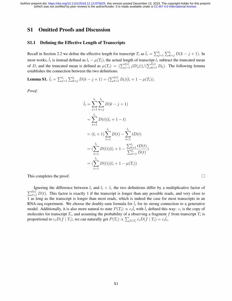
Recall in Section 2.2 we define the effective length for transcript Ti as li =∑li

j=1

∑lik=j D(k − j + 1). In

most works, li is instead defined as li − µ(Ti), the actual length of transcript li subtract the truncated meanof D, and the truncated mean is defined as µ(Ti) = (

∑l(i)j=1 jD(j))/(

∑l(i)k=1Dk). The following lemma

establishes the connection between the two definitions.

Lemma S1. li =∑li

j=1

∑lik=j D(k − j + 1) = (

∑l(i)t=1Dt)(li + 1− µ(Ti)).

Proof.

li =

li∑j=1

li∑k=j

D(k − j + 1)

=

li∑t=1

D(t)(li + 1− t)

= (li + 1)

li∑t=1

D(t)−li∑t=1

tD(t)

= (

li∑t=1

D(t))(li + 1−∑li

t=1 tD(t)∑lit=1D(t)

)

= (

li∑t=1

D(t))(li + 1− µ(Ti))

This completes the proof.

Ignoring the difference between li and li + 1, the two definitions differ by a multiplicative factor of∑l(i)t=1D(t). This factor is exactly 1 if the transcript is longer than any possible reads, and very close to

1 as long as the transcript is longer than most reads, which is indeed the case for most transcripts in anRNA-seq experiment. We choose the doubly-sum formula for li for its strong connection to a generativemodel. Additionally, it is also more natural to state P (Ti) ∝ ci li with li defined this way: ci is the copy ofmolecules for transcript Ti, and assuming the probability of a observing a fragment f from transcript Ti isproportional to ciD(f | Ti), we can naturally get P (Ti) ∝

∑f∈Ti ciD(f | Ti) = ci li.

S1


https://doi.org/10.1101/2019.12.13.875625


S1.2 Re-calculating Normalization Constant

In this section, we prove the following equation, which is necessary for the reparameterization processdescribed in Section 2.2:∑

Ti∈Tlici =

∑Ti∈T

li∑j=1

li∑k=j

D(k − j + 1)ci

=∑p∈P

∑i,j,k:p(Ti[j,k])=p

D(k − j + 1)ci

=∑p∈P

(∑

j,k:∃i,p(Ti[j,k])=p

D(k − j + 1))(∑

i:p⊂p(Ti)

ci)

=∑p∈P

lpcp

The third equation holds because the sum of D(k − j) across any transcripts containing path p is the same,as shift in reference does not change D(k − j).

S1.3 Trimming Set of Phasing Paths

Recall the likelihood function under our reparameterized model: P (F | T , c) ∝∏f∈F cp(f)/(

∑p∈P cp lp).

Paths p ∈ P with no mapped reads do not contribute to∏f∈F cp(f), as there are no f ∈ F such that

p(f) = p. It does play a role in calculating the normalization constant∑

p∈P cp lp. However, since we onlyremove paths with very low lp, the contribution of cp lp for this set is intuitively small. This removal thuscauses small underestimation of the normalization constant, and in turn small overestimation of transcriptabundances (and path abundances).

If there is a removed path with large cp when optimized under the full model, it means in the inferredtranscriptome there is a lot of reads mapped to path p, even though zero reads mapped in the sequencinglibrary. This mostly happens if there is a dominant transcript with incredibly high abundance, and p is partof the transcript. For such things to happen, the transcript must have huge amount of reads mappable, andthe fact that no a single read mapped to path p indicates lp is incredibly small, or the modeling might befaulty.

This trimming is necessary as the fragment length distributionD(l) usually has a long tail when inferredfrom experiments, due to smoothing and potential mapping errors, leading to a lot of extremely long pathsthat are near impossible to sample a read from. This trimming might have some effect on our analysis ofnon-identifiability later from a theoretical perspective, as intuitively by trimming down P we are increasingthe co-dimension of {cp} in {ci} leading to wider ranges of optima. However, as we described above, it isnear impossible to sample a read from such paths, unless we have infinite amount of data, which is not thecase in practice. In other words, the trimming can be seen as a modification to the original likelihood modelto account for the fact that we cannot generate infinitely large sequencing libraries.

S1.4 Path Dependent Bias Correction

Our proposed model is also capable of bias correction, but not to the full extent as done in Salmon. We definethe affinityAp(j, k) as the unnormalized likelihood of generating a read pair mapped to path p from position

S2


https://doi.org/10.1101/2019.12.13.875625


j to k in some coordinate. This is the analogue for P (fj | ti) in Salmon model, excluding the sequencespecific terms (which can also be integrated into our model directly, but they will not appear in effectivelength calculation). For non-bias-corrected model, we simply have Ap(j, k) = D(k − j + 1). The biascorrection that can be applied directly are then those calculated from the genomic sequence in between thepaired-end alignment, including certain motif-based correction and GC-content-based correction. To adaptthe likelihood model with bias correction, the definition of transcript and path effective length is changed asfollows:

li =

li∑j=1

li∑k=j

Ap(Ti[j,k])(j, k)

lp =

li∑j=1

li∑k=j

Ap(j, k)1(p(Ti[j, k]) = p),∀p ∈ p(Ti)

Note that lp is the same for any Ti and we assume the coordinate when calculating Ap coincides withthe internal coordinate of Ti. The definition of path abundance remains unchanged, and the inference andsubgraph quantification processes are the same.

Admittedly, there is no way to know the exact location of the read pair within the transcript after repa-rameterization with path abundance, so transcript-specific bias correction cannot be done in an exact manner.Nonetheless, since the splice graph is known in full, approximate bias correction is possible. In our exper-iments, let Ai(j, k) denote the affinity value calculated from a full bias correction model, for the fragmentgenerated from base j to k on transcript Ti. Let ri be the reference abundance of transcript Ti. Then welet Ap(j, k) = (

∑i:p⊂p(Ti) riAi(j

′, k′))/(∑

i:p⊂p(Ti) ri), where j′ and k′ are the coordinates of the pathsequence in reference coordinate of Ti. If Ai(j, k) is independent of transcript i but only dependent on thepath p, we have Ap(j, k) = Ai(j

′, k′) for any transcript i containing path p. Otherwise, we average theaffinity value calculated from known transcripts on this loci, weighted by their reference abundance. Forsimplicity, we use Salmon outputs as reference abundance, but other approaches, including iterative processof estimating Ai(j, k) and cp alternatively, are possible.

One limiting factor for bias correction is that calculating lp can be expensive as we need to calculate thisfor every possible fragments. To speed up this process, we can use a simplified form for Ap(j, k) so lp hasa closed-form solution (for example, do not allow bias correction when calculating effective length, similarto existing approaches to calculate effective length of transcripts), sample from possible Ap(j, k) when thenumber of fragments from a particular path is large, or precompute the values for fixed genome and biascorrection model. These approaches may result in slightly inaccurate path effective length, and it is still anopen question how it affects downstream procedures.

S1.5 Compact Aho-Corasick Automaton and Compact Prefix Graph

In this section, we formally define the ingredients of prefix graph flows and prove several claims in the maintext in a more rigorous manner based on a more compact construction.

Definition S3 (Aho-Corasick CFSA for phasing path matching). The Compact Aho-Corasick Finite-StateAutomaton (CFSA) is built with the following setup:

• The alphabet is the set of all vertices in splice graph.

S3


https://doi.org/10.1101/2019.12.13.875625


• The patterns to match against is the union of (1) all paths of length 1, and (2) all path in P with lastexon removed.

• The dictionary suffix link d[s, a], where s is a state in the FSA and a is a character (vertex in splicegraph in our case), is calculated if and only if there is an edge from last vertex in s to a.

• Additionally, each suffix link is labelled with sa, the path represented by s attached by a, which byour construction is still a valid path in the splice graph.

• A path p in P is said to be recognized at a suffix link with label s′, if p is a suffix of s′.

Intuitively, we wasted some space in the original prefix graph by only using vertex-level informationwhen the edge-level information are also available. The “compact” in the name of this CFSA is for the factthat not all dictionary suffix links are calculated as in usual Aho-Corasick FSAs, and the fact that patternrecognition happens over transitions (suffix links), not states. We construct the prefix graph in the same wayas in the main text, extracting states of the CFSA as vertices and dictionary suffix links as edges, excludingthe initial state where no suffix is matched. We call this new graph a compact prefix graph. For the rest ofthis section, we use {cs} to denote a flow on the compact prefix graph.

Lemma S2 (Properties of Compact Prefix Graph). Given a compact prefix graph and a flow {cs} mappedfrom a transcriptome {Ti, ci}:

• The compact prefix graph is a DAG.

• There is a one-to-one mapping between S − T paths in splice graph and [S]− [T ] paths in compactprefix graph.

• The value {cp} can be derived from the compact prefix graph alone, and is preserved during mappingbetween compact prefix graph flows and transcriptomes (similar to the main text): cp =

∑i:p⊂p(Ti) ci.

Proof. • We label each node in the prefix graph by the last vertex of their corresponding CFSA state. Ifan edge goes from u to v (two nodes in the compact prefix graph), there is an edge from the label ofu to the label of v (two nodes in the splice graph). This means we can sort the nodes of the compactprefix graph by using the label and the topological order of the splice graph, breaking ties arbitrarily,and the result will be a valid topological order for the compact prefix graph.

• For a [S]− [T ] path of the compact prefix graph, we can generate the path on splice graph by writingdown the label for each node (as defined above, last vertex in the representing string). The resultingpath is valid on the splice graph. On the other hand, we can generate a path on the compact prefixgraph by feeding the transcript to the CFSA and list the visited states in CFSA.

• We need to show that exactly one edge in the set AS(p) is visited if a transcript T matches p. This isthe transition right before the last exon in p is visited, so it happens exactly once as no exon can bevisited twice. The rest of the proof is identical to the original prefix graph proof.

There are many other methods to achieve the same end result of representing {cp}. For example, sim-ply have a variable ci for each possible transcript, representing the transcriptome in its original form, andcalculate the path abundance by definition. However, the compact prefix graph formulation is the simplestpossible in certain sense, as shown in the following theorem:

S4


https://doi.org/10.1101/2019.12.13.875625


Theorem S2 (Compact Prefix Graph Flow can be Minimal Sufficient). With fixed splice graph and pathset P , if P satisfy the condition that for each p ∈ P any prefix of p is also in P , there is a one-to-onemapping between feasible set of {cp | p ∈ P} and feasible set of {cs} where s iterates over the set of edgesof compact prefix graph.

Proof. The mapping from a compact prefix graph flow to {cp} is direct and unique. For the other direction,assuming the theorem is false, there exists two sets of {cs}, compact prefix graph flow with identical {cp}.Since each cp is sum of several flow values, the difference between the sets {∆cs} satisfies the following:∑

s∈AS(p)

∆cs = 0, ∀p ∈ P

We now prove that ∆cs = 0 for all s, using induction on the size of s (length of the splice graph path itrepresents), which we denote k. The induction hypothesis for k is that ∆cs = 0 for all edge s with size noless than k. For the base case where k > maxs |s|, there are no edges with size k or larger, so the hypothesisholds trivially. Assume this holds for k + 1. For each edge s′ with size k, denote the splice graph path itrepresents as p′. By the construction of CFSA, it is a prefix of some p′′ ∈ P , and by the setup of the theoremp′ ∈ P , which means there is a corresponding equation

∑s∈AS(p′) ∆cs = 0. The set AS(p′) contains the

edge s′ (by definition) and some edge whose represented path is longer than s′, and for all edges in the lattercategory, the induction hypothesis says their ∆cs = 0. This means ∆cs′ for the edge we are looking at isalso zero.

S1.6 Localized Expectation-Maximization

In this section, we rewrite the optimization target in a slightly different form: we optimize∑

f∈F log cp(f)

satisfying∑

p∈P cp lp = 1. The resulting maximum likelihood will be the same in both formulations, butcp might be scaled by a constant between the optimal solutions. We also exclusively use the compact prefixgraph defined in Section S1.5, and call it prefix graph for brevity.

We first look at multimapped reads. Let M(f) denote the set of paths that a read pair f can map to,D(f | p) be the fragment length probability when read pair is mapped to path p, the objective functionbecomes:

logP (F | T, c) =∑f∈F

log(∑

p∈M(f)

cpD(f | p))

and the constraints being the same as before. First, with a standard EM argument, we can define allocationvariable z and perform the following EM step:

E-step:zf,p = c′pD(f | p)/(∑

p′∈M(f)

c′p′D(f | p′))

M-step:c = arg maxc

∑p∈P

(∑f∈F

z′f,p) log cp

c′ and z′ denote values from last iteration. In the M-step the variable c also needs to satisfy aforementionedprefix graph constraints, including

∑p∈P cp lp = 1.

Next, we adapt our EM algorithm to optimize over multiple genes at once. Let g denote a gene and Pgdenote the set of paths belonging to g. The target function during the M-step can be decomposed by genes,

S5


https://doi.org/10.1101/2019.12.13.875625


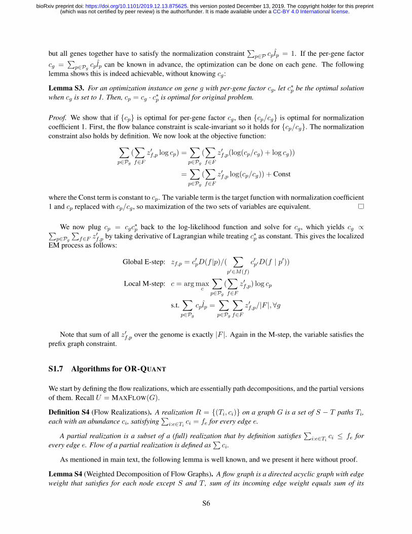
but all genes together have to satisfy the normalization constraint∑

p∈P cp lp = 1. If the per-gene factorcg =

∑p∈Pg

cp lp can be known in advance, the optimization can be done on each gene. The followinglemma shows this is indeed achievable, without knowing cg:

Lemma S3. For an optimization instance on gene g with per-gene factor cg, let c∗p be the optimal solutionwhen cg is set to 1. Then, cp = cg · c∗p is optimal for original problem.

Proof. We show that if {cp} is optimal for per-gene factor cg, then {cp/cg} is optimal for normalizationcoefficient 1. First, the flow balance constraint is scale-invariant so it holds for {cp/cg}. The normalizationconstraint also holds by definition. We now look at the objective function:∑

p∈Pg

(∑f∈F

z′f,p log cp) =∑p∈Pg

(∑f∈F

z′f,p(log(cp/cg) + log cg))

=∑p∈Pg

(∑f∈F

z′f,p log(cp/cg)) + Const

where the Const term is constant to cp. The variable term is the target function with normalization coefficient1 and cp replaced with cp/cg, so maximization of the two sets of variables are equivalent.

We now plug cp = cgc∗p back to the log-likelihood function and solve for cg, which yields cg ∝∑

p∈Pg

∑f∈F z

′f,p by taking derivative of Lagrangian while treating c∗p as constant. This gives the localized

EM process as follows:

Global E-step: zf,p = c′pD(f |p)/(∑

p′∈M(f)

c′p′D(f | p′))

Local M-step: c = arg maxc

∑p∈Pg

(∑f∈F

z′f,p) log cp

s.t.∑p∈Pg

cp lp =∑p∈Pg

∑f∈F

z′f,p/|F |, ∀g

Note that sum of all z′f,p over the genome is exactly |F |. Again in the M-step, the variable satisfies theprefix graph constraint.

S1.7 Algorithms for OR-QUANT

We start by defining the flow realizations, which are essentially path decompositions, and the partial versionsof them. Recall U = MAXFLOW(G).

Definition S4 (Flow Realizations). A realization R = {(Ti, ci)} on a graph G is a set of S − T paths Ti,each with an abundance ci, satisfying

∑i:e∈Ti ci = fe for every edge e.

A partial realization is a subset of a (full) realization that by definition satisfies∑

i:e∈Ti ci ≤ fe forevery edge e. Flow of a partial realization is defined as

∑ci.

As mentioned in main text, the following lemma is well known, and we present it here without proof.

Lemma S4 (Weighted Decomposition of Flow Graphs). A flow graph is a directed acyclic graph with edgeweight that satisfies for each node except S and T , sum of its incoming edge weight equals sum of its

S6


https://doi.org/10.1101/2019.12.13.875625


outgoing edge weight. Every flow graph can be decomposed into finite number of S − T paths {Ti} withweight {ci} where

∑i:e∈Ti ci = fe holds for every edge e.

With inferred flows, prefix graph G is a flow graph that can be decomposed into a finite number ofweighted paths. OR-QUANT problem asks for the minimum and maximum flow of a partial realization ofwhich the paths go through any edge in E′. We now state our algorithms and prove their correctness.

Theorem S3 (Diff-Flow). The auxiliary graph G− is built with edge set E − E′.

Z = U −MAXFLOW(G−) is tight lower bound for OR-QUANT of E′.

Proof. We prove the theorem in two parts: First, we show there is a realization r of G such that Q(r) =U −MAXFLOW(G−), then we show any realization satisfies Q(r) ≥ U −MAXFLOW(G−).

The key observation is that all S − T paths that do not include any edge in E′ are represented as fullpaths in G−. For the first part, fix a maximum flow of G− as F−, we first build a realization r− from F−,then build a realization r+ from the graph G−F−. We have Q(r−) = 0, as no path in r− contain any edgein E′. The flow of r+ is exactly Z = U − MAXFLOW(G−), so Q(r+) ≤ Z and equation holds if everypath in r+ intersect with E−. If some path in r+ does not intersect with E′, F− is not a maxflow of G−,because we can add that path to F− to improve the flow, leading to a contradiction. This means every pathin r+ intersects with E′, so q(r+) = U − MAXFLOW(G−) and a full realization r = r+ + r− have thedesired property.

Similarly for the second part, for any realization r we split it into two parts: r+ containing set of pathsthat intersect with E′, and r− containing everything else. r− is a flow on G−, so its flow cannot exceedMAXFLOW(G−). This means Q(r) = Q(r+) = U −Q(r−) ≥ Q−MAXFLOW(G−) = Z.

Theorem S4 (Split-Flow). The auxiliary graph G∗ is built by adding a vertex T ′ in G and for each edge inE′ changing its destination to T ′. T ′ replaces T as the sink of flows.

Y = MAXFLOW(G∗) is tight upper bound for OR-QUANT of E′.

Proof. We prove the theorem in a similar style: First we show there is a realization r of G such that Q(r) =MAXFLOW(G∗), then we show any realization satisfies Q(r) ≤ MAXFLOW(G∗).

For the first part, we first build realization r∗ from a maximum flow of G∗. However, r∗ is not a validrealization on G, because G∗ and G have different sets of edges. Our goal is to get a realization r+ of Gthat is a “reconstruction” of r∗ on G.

For convenience, we define the following:

Path Mapping for G∗. A S − T path on G is mapped to a S − T ′ path on G∗ by finding first edge ofthe path that is in E′, change the destination of that edge to T ′, and discard the path after that edge (so thepath ends at T ′). The original path is guaranteed to intersect with E′.

Similarly, a S − T ′ path on G∗ is mapped to a path on G by moving the destination of last edge (thatwas T ′) back to its original node before the transformation. We assume a label is kept on each edge thatends at T ′, so multiple edges can exist between a node and T ′. The resulting path is guaranteed to intersectwith E′, but is not a complete S − T path.

We apply an induction argument, formally defined as follows:

S7


https://doi.org/10.1101/2019.12.13.875625


Flow Reconstruction Instance. An instance for flow reconstruction has two inputs: (F, r∗). F is aflow on G (they share the same topology but not flow values), and r∗ is a partial realization on F ∗, whereF ∗ is constructed in the same way as G∗ by moving endpoints of edge in E′ to a new node T ′. The outputof the instance is r+, a partial realization of F , satisfying the condition that (1) each path in r+ intersectswith E′, and (2) if we map each path in r+ back to F ∗, resulting realization r∗+ has the same flow as r∗.

The size of a flow reconstruction instance is defined as the size of r∗ (number of paths), not to beconfused with the flow of the instance. Our goal is to solve the instance for any size. The base case is whenthe size is zero meaning r∗ is empty, and an empty r+ can be returned. Now assuming the instance can besolved for size less than k, we solve the instance for size k.

Induction Algorithm. Pick the path (P, c) in r∗ whose second-to-last node (right before T ′) is the lastamong all paths in topological ordering of G. Denote the last edge of this path, mapped back to F , as (u, v).P without last edge is then a path from S to u.

We next generate an arbitrary realization of F and use it to construct the a partial realization that roughlymatches (P, c). To do this, we first discard paths that do not contain edge (u, v) in the realization. Then, forevery remaining path in the partial realization, we change its path before u to match P and scale the weightby c/w where w is the flow of edge (u, v) on F . Note that c/w ≤ 1, because r∗ is a partial realization onF ∗, meaning the flow of P does not exceed the flow on the edge (u, T ′) that was mapped from (u, v), whichhas capacity exactly w.

Denote the scaled partial realization as r0. r0 has total flow c, is a valid partial realization of F , andevery path in r0 has P (mapping its last edge back to G as (u, v)) as prefix. We continue mapping the pathsby recursively calling the procedure on (F ′, r′∗), where F ′ is F with flow of r0 subtracted (as c/w ≤ 1, F ′

is still a valid flow graph), and r′∗ is r∗ with (P, c) removed.

Proof of Induction Correctness. The new instance to be called is an instance with size k−1, since onepath in r∗ is removed. We first prove the recursive call is valid, that is, r′∗ is indeed a partial realization ofF ′∗.

If this call is invalid, it means some edge in F ′∗ has less flow than the cumulative flow from r′∗. Since r∗

is a partial realization of F ∗ and r′∗ is a subset of r∗, this can only happen to some edge that is in a path in r0

(only for these edges F ′∗ have less flow than F ∗). By construction of r0, this edge can only be either someedge in P (including the edge (u, v)), or some edge whose starting point is later than v in topological orderof G. For the former case, exactly c flow is subtracted on this edge from F to F ′, and it is the same from r∗

to r′∗ for the path is removed with weight c. For the latter case, note that such edge have nonnegative flowin F ′∗ but zero flow in r′∗, otherwise this means some path in r∗ uses that edge, which contradicts with ourselection criteria of (P, c).

Given the recursive call is valid, we can prove the correctness of the algorithm by showing that r+

indeed satisfies the two output conditions. For (1), each path in r+ contains some edge (u, v) as defined inthe induction algorithm, which is in E. For (2), note that at each recursion call, the realization r0 mapped toF ∗ matches the flow of one path (P, c) in r∗, so the condition is maintained in recursion. This finishes thecorrectness proof for the induction.

Completing the Proof. With the induction algorithm, we can reconstruct a partial realization r+ of Gfrom r∗ that is realization of a maxflow onG∗, then similar to last proof, construct r− fromGminus the flowof r+. By construction of r+, we have Q(r+) = MAXFLOW(G∗). If some path in r− intersect with E′, wecan map that path to G∗ and improve the maxflow that yields r∗, contradiction. This means Q(r−) = 0 andQ(r) = MAXFLOW(G∗).

S8


https://doi.org/10.1101/2019.12.13.875625


On the other hand, for a realization r of G, we can write r = r+ + r− where r+ contains transcriptsthat intersect with E′, and r− otherwise. We can map each path in r+ to G∗ and resulting realization r∗ isa flow on G∗, so Q(r) which is total flow of r+ cannot exceed MAXFLOW(G∗). This completes the wholeproof.

S1.8 Algorithms for AND-QUANT

We start by discarding any edges e ∈ El such that there are no S − T path t satisfying e ∈ t and |t ∩Ek| >0,∀k, and assume the remaining edge set is not empty. By definition, removal of these edges will not changethe answer to AND-QUANT.

Definition S5 (Start/End-Sets and Natural Order). Define Ui = {u : (u, v) ∈ Ei}, Vi = {v : (u, v) ∈ Ei}and for convenience, V0 = {S}, Um+1 = {T}.

Since G is a DAG, we also define the natural order u ≤ v if there is a directed path starting at u andending at v. We define x → Vi as the condition that there is some vi ∈ Vi such that x ≤ vi (intuitively, xcan reach Vi). Same goes for Ui and the other direction.

Theorem S5 (Block-Flow). DefineBi, the ith block subgraph, the set of edges (u, v) that satisfies Vj−1 → uand v → Uj , for 1 ≤ i ≤ m+ 1. The full block graph GB is the union of all Bi and Ei.

MAXFLOW(GB) is the tight upper bound for AND-QUANT of {Ek}.

The auxiliary graph G+B is built by using the construction in Split-Flow, replacing E′ by GB .

MAXFLOW(G+B) is the tight lower bound for AND-QUANT of {Ek}.

The proof of Block-Flow theorem is essentially a complementarity argument, as shown in the followinglemmas.

Lemma S5 (Well-Order Property). If u ∈ Ui, v ∈ Vj , v ≤ u, then i > j.

Proof. We can derive this from the well-order property of {Ek}. v ≤ u means there is a path that visits anedge in Ej then an edge in Ei, as there exists a path from S to an edge in Ej using v, and a path from anedge in Ei using u to T .

Lemma S6. For each vi ∈ Vi, vi → Ui+1.

Proof. Recall that we removed all edges in Ei that does not belong to any of paths that would satisfy thequantification criteria. vi ∈ Vi implies there is an edge (ui, vi) ∈ Ei that is contained in such a path, sothere is some edge (ui+1, vi+1) after it, which implies vi → Ui+1.

As a corollary, this means if ui ∈ Ui then ui → Uj where j > i, because there exists vi such that(ui, vi) ∈ Ei and vi → Uj . Same goes for Vi.

Lemma S7. For a fixed i, each vertex x in GB either satisfies x→ Ui or Vi → x, but not both.

Proof. x is in GB because there is a path that use x and satisfy the quantification criteria: This holds if xis in any Ei, and if x is in any of Bi, by definition of Bi there is a path from some vj−1 to ui that includes

S9


https://doi.org/10.1101/2019.12.13.875625


x, and we can extend both ends for a path that satisfies the criteria. The path uses some edge in Ei, anddepending on whether x appears before Ei or after Ei it satisfies either x→ Ui or Vi → x.

No vertices can satisfy both, otherwise we have u ∈ Ui, v ∈ Vi and v ≤ x ≤ u, which would implyi < i, contradiction.

Lemma S8 (Main Lemma for AND-Quant). An S − T path in G satisfies the quantification criteria if andonly if it is a subset of GB .

Proof. We first prove that if a path satisfies the quantification criteria, it is within GB . An edge (u, v) onthe path is either in some Ei, or between some edge in Ei−1 and some edge in Ei; In latter case, we knowVi−1 → u and v → Ui, which directly imply (u, v) ∈ Bi.

To prove the other direction, we show that removing each of Ei results in disconnection of S to T . Bythe previous lemma, the vertices of GB can be partitioned as: S = {x : x→ Ui, x ∈ GB}, T = {x : Vi →x, x ∈ GB}. Consider an edge (u, v) ∈ GB that starts in S and ends in T :

• If (u, v) ∈ Bj , we know Vj−1 → u→ Ui, so j − 1 < i, and at the same time Vi → v → Uj so i < j,but there is not an integer i between j − 1 and j, contradiction.

• If (u, v) ∈ Ej , we know Uj → u → Ui so j ≤ i (because Vj−1 → u), and Vi → v → Vj so i ≤ j(because v → Uj+1), which implies i = j.

So we have (u, v) ∈ Ei. In other words, removing all edge in Ei results in disconnection between S and T ,so each S − T path in GB uses an edge in Ei, for each i. This means the path satisfies the quantificationcriteria.

The last lemma means that all path that does NOT satisfy the AND-QUANT criteria intersects withG − GB , meaning that we can complement the result of OR-QUANT on E′ = G − GB to get the desiredresult. This completes the proof for the main theorem.

S1.9 Subgraph Quantification with Flow Reallocation

When we do subgraph quantification, we are finding path decompositions over prefix graph flows. As weproved before, if P satisfies a regularity constraint, the compact prefix graph (defined in Section S1.5) flowskeep track of exactly the set of path abundance that is required for the likelihood. However, if this conditionfails, the compact prefix graph flow is keeping more path abundance than necessary: these are the pathsthat are prefix of some other paths in P , but not in the set itself. The fact that we can calculate cp for suchpaths from the compact prefix graph alone indicates a narrower range in subgraph quantification, becausewe implicitly add extra constraints to the recovered transcriptome.

This constraint can be removed. For each of the subgraph quantification algorithms, we calculate a

S10


https://doi.org/10.1101/2019.12.13.875625


MAXFLOW of f , a flow over some variant of the compact prefix graph, which can be written in an LP form:

max∑

e∈Out(S)

f ′e

s.t.∑

e∈Out(v)

f ′e =∑

e∈In(v)

f ′e, ∀v ∈ V − {S, T}

0 ≤ f ′e ≤ fe, ∀e ∈ E

where fe is determined from the compact prefix graph flow and the corresponding algorithm. However, wedo not care about the exact compact prefix graph flow, as the path abundances {cp} determine the likelihoodof the model. In a similar spirit with the reallocation process under complete reference assumption (Section2.2), we propose to reallocate the flow of prefix graph as an LP. This results in the following LP, where sdenotes an edge in compact prefix graph, {c∗s} is the original compact prefix graph flow modified by theproblem of interest, and {cs} is the re-estimated flow:

max∑

s∈Out([S])

cs

s.t.∑

s∈Out(v)

cs =∑

s∈In(v)

cs,∀v ∈ V − {[S], [T ]}

∑s∈AS(p)

cs =∑

s∈AS(p)

c∗s,∀p ∈ P

0 ≤ cs ≤ c∗s, ∀s

In experiments we only report the bounds without this flow-re-estimation step because the effect is small.The idea of re-expressing maxflows as LPs is very powerful and possibly enables other extensions of sub-graph quantification, but at the cost of higher computational complexity.

S1.10 Flow Inference with Partial Reference Completeness Assumptions

By expressing lλ as an affine combination of l0 and l1, we implicitly assume every read is split into a readwith count λ that would be from any transcript with known junctions, and a read with count 1−λ that wouldbe from the reference transcriptome. Such modeling might not be ideal for some applications. A naturalalternative is to assume that λ portion of all reads would come from any transcript with known junctions,while 1 − λ portion would be from the reference. In this section, we show how to extend our methods forthis alternative assumption by an alternative inference procedure. Note that in our original modeling, weonly need to run inference for λ = 1, so this method is inherently more costly as we need to run an inferenceinstance for every λ in consideration. In addition to the flow values, for each reference transcript Ti, we adda variable ci denoting its abundance, and change the formula of cp as follows:

cp =∑

s:s∈AS(p)

f(s) +∑

i:p⊂p(Ti)

ci

. We change the normalization term (which was∑

p∈P cp lp = 1) as follows:∑p∈P

cp lp = λ,∑Ti∈T

ci li = 1− λ

S11


https://doi.org/10.1101/2019.12.13.875625


. The resulting optimization program would quantify the transcripts assuming at least 1−λ portion of readscome from known transcripts. For genome-wide quantification, the same local-global EM algorithm can beused assuming λ for each gene stay unchanged. For calculation of range of optima, we use the reallocationLP on {ci} and subgraph quantification on {cp}, then add the results together. This method is still limited inthe sense that we have to make the assumption on a per-gene basis, and cannot model the scenario where weassume λ portion of the whole read library come from novel transcripts (which requires a huge optimizationinstance as discussed in Section 2.4). In practice, we stick to the simple affine combination of l0 and l1

as it is the most efficient, however, the algorithm presented in this section might be interesting for futureextensions of the model.

S2 Supplementary figures

0

1000

2000

3000

4000

lower bound 50% upper bound

quantile

coun

t

quantile of Salmon point estimates within uncertainty range

A

0

1000

2000

3000

4000

1.0 2.5 10.0 100.0 1000.0 10000.0

ratio

coun

t

ratio between upper bound and Salmon point estimates

B

Assumptioncomplete referenceincomplete reference

Figure S1: (A) Histogram of the position of Salmon estimates within the range of optima. X axis is thepercentile between the lower bound and the upper bound of the range of optima. (B) Histogram of ratiobetween upper bounds and Salmon estimates.

S12


https://doi.org/10.1101/2019.12.13.875625


0.0

0.2

0.4

(0,lower bound) [lower bound, upper bound] (upper bound, infinity)

Per

cent

age Type

zero certain boundsnonzero certain boundsuncertain bounds

Percentage of Salmon estimates below, within and above the bounds under incomplete reference assumption

Figure S2: Percentage of Salmon estimates that are below the lower bounds, between the lower and upperbounds, and above the upper bounds of the uncertainty range under the assumption of freely expressed splicegraph paths. That Salmon estimates are outside the uncertainty range can be explained by the differencebetween optimal objectives under different parameter spaces: the parameter space of Salmon is annotatedtranscripts and the one under the incomplete reference assumption is all paths in the splice graph.

S13


https://doi.org/10.1101/2019.12.13.875625


finding ranges of optimal transcript expression ... · 12/13/2019 · tions, especially under the...

Documents