finding order in chaos: a behavior model of the whole grid

Finding order in chaos: Abehavior model of the wholegrid

Jesus Montes1∗, Alberto Sanchez2, Julio J. Valdes3, Marıa S. Perez4 and PilarHerrero4

1 Centro de Supercomputacion y Visualizacion de Madrid (CeSViMa),Universidad Politecnica de Madrid,Parque Tecnologico UPM, Pozuelo de Alarcon,Madrid, Spainemail: [email protected] E.T.S. de Ingenierıa Informatica, Universidad Rey Juan Carlos,Campus de Mostoles, Mostoles,Madrid, Spainemail: [email protected] Research Council Canada,Institute for Information Technology,M50, 1200 Montreal Rd,Ottawa, ON K1A 0R6, Canadaemail: [email protected] de Informatica, Universidad Politecnica de Madrid,Campus de Montegancedo s/n, Boadilla del Monte,Madrid, Spainemail: [email protected], [email protected]

SUMMARY

Over the last decade, grid computing has paved the way for a new level of large scaledistributed systems. However, this new step in distributed computing comes along with acompletely new level of complexity. Grid management mechanisms play a key role, and acorrect analysis and understanding of the grid behavior is needed. Traditional distributedcomputing management mechanisms analyze each resource separately and adjust specificparameters of each one of them. When trying to adapt the same procedures to gridcomputing, the vast complexity of the system can complicate this task.

But grid complexity could only be a matter of perspective. It could be possible tounderstand the grid behavior as a single system, instead of a set of resources. Thisabstraction could provide a deeper understanding of the system, describing large scalebehavior and global events that probably would not be detected analyzing each resource

∗Correspondence to: [email protected]

FINDING ORDER IN CHAOS: A BEHAVIOR MODEL OF THE WHOLE GRID 1

separately.

In this paper a specific methodology is presented and described in order to create aglobal behavior model of the grid, analyzing it as a single entity. Both real and simulatedcase studies are also presented, in order to provide a proper validation and illustrate thebenefits of this approach.

key words: Large-scale dsitributed systems, Grid computing, Modelling, Data mining, Grid behavior

1. Introduction

Grid technology [19] provides access to a pool of geographically distributed computing anddata heterogeneous resources. Although nowadays it is achieving its maturity, the architecturalcharacteristics of the environment (like the use of these heterogeneous elements, security relatedissues, asynchronism, scalability and the coordinated use of non-dedicated resources) can causemanagement and reliability problems†. The complexity of this kind of environments makesit very difficult to optimally take advantage of its capabilities in order to execute highlysophisticated applications. Dealing with this complexity becomes a major priority, in order tomanage the environment and make decisions aimed at using the resources in a better way.

The high level of sophistication of grid environments requires to find new ways to managethem. Nevertheless, it is required to understand properly the environment before trying toimprove its management. The traditional and current vision of grid management [3, 31, 48]tries to understand the environment from the behavior of the set of its independent andheterogeneous resources. This implies that current grid management techniques require a deepknowledge about the operation of each grid resource. However, the diversity, dynamism andhuge size of the information collected for all the parameters required to manage each resourcemake grid understanding difficult. Therefore, a new approach to simplify it without losinginformation which is relevant would be very beneficial to manage the system.

With this aim, we propose to break with the traditional philosophy of grid management,considering aspects according to the whole system behavior instead of each grid resourceoperation. This way, grid management is based on a behavior abstraction of the whole systemas a single entity instead of specific information about each and every element that togetherform the environment. In this paper, we present our approach which models a grid as a whole,with the aim of simplifying its management and decision making. This model is extracted fromthe analysis of monitored data along a large period of time. The model can help the scientificcommunity to tackle different problems that are currently not properly solved in the grid field.

†Note that a a grid is defined as a system that coordinates resources that are not subject to centralized control[18].

Copyright c© 2009 John Wiley & Sons, Ltd. Concurrency Computat.: Pract. Exper. 2009; 0:0–0Prepared using cpeauth.cls

2 J. MONTES ET AL.

Fault tolerance and job scheduling adapted to the dynamic changes and behavior of the wholegrid can be hightlighted among others.

The paper is organized as follows. Section 2 shows different works related to our approach.Section 3 proposes a methodology designed to obtain a global behavior model of large scaledistributed environments, like a grid. Section 4 shows a generic framework for addressing thisproblem. Section 5 validates our proposal by means of the evaluation of both a simulatedcase study and a real grid environment. Finally, Section 6 summarizes the conclusions of theanalysis performed and outlines the future research lines.

2. Related Work

Several initiatives aim to model and characterize the behavior of a grid. Benchmarks [11]are common solutions used for characterizing the performance behavior of a system underrepresentative workloads. With the use of benchmark programs, a performance model of thesystem can be obtained. Many advances have been achieved in the field of grid benchmarking[10]. Different grid benchmarking approaches have been developed: NAS Grid Benchmark(NGB)[21] and GridBench [49], among others. However, grid benchmarking cannot model andpredict the dynamic behavior of grids. Another disadvantage of grid benchmarking techniquesis their dependence on the accuracy of benchmarks and the suitable selection of inputs andconfiguration parameters. Since the results are not based on real data over the grid, theselection of a realistic workload is a critic step.

Bratosin et al. [2] offer a formal description of grids by means of Colored Petri Nets (CPN).In this way, a grid can be simulated. Our proposal is not a simulation of a grid but a simplifiedmodel of a specific grid environment, which makes easier the application of more efficientmanagement techniques.

Nemeth et al. [37, 36] state the differences between grids and conventional distributedenvironments. With this aim, they show a high level semantical model for grids by meansof the use of Abstract State Machines (ASM) [23], a mathematical framework for analysisand design of systems. Nevertheless, this definition takes only into account the qualitativecharacteristics of an ideal grid.

Palatin et al. [41] apply data mining techniques in the creation of a distributed outliersdetection algorithm, which allows researchers to understand the grid resources behavior anddetect possible machine misconfigurations. Unlike this approach, our proposal is a genericmechanism that provides a global understanding of the grid by means of the use of knowledgediscovery techniques.



3. A global behavior model for understanding the grid

As it has been said, usual grid management mechanisms try to improve performance basedon the individual analysis of every component on the system. Then they try to adjust theconfiguration or predict the behavior of each independent element. This approach may seemreasonable considering the large scale and complexity of the grid. However it could possiblyfail to achieve optimal performance, because in most cases it lacks the capability to understandthe effects that different elements have on each other when they work together. From a moretheoretical point of view, if we consider a grid as an individual entity (with its computationalpower, storage capacity and so on), it seems logical to analyze it as such, instead of composedof a huge set of individual resources. Therefore two different ways of of understanding the gridcan be distinguished. First of all, the “multiple entity” point of view, common in most gridmanagement techniques, where the system is controled analyzing each resource independently.On the other hand, there is also the “single entity” point of view, in which the grid is regardedas a single system (the grid). This is similar as how computers are regarded as individualentities, even though they are made of several electronic components of different nature, orhow clusters are most times considered as single machines, when in fact they are composedby many computers. It is, finally, a matter of abstraction, and a global behavior model of agrid would provide the necessary abstraction layer that finally makes the single entity pointof view possible.

In order to do so, a behavior model for the whole grid must have certain characteristics:

• Specific state definition: State characteristics and transition conditions should beunambiguously specified. The number of states should also be finite, in order to providea useful model. A typical model representation that fits with these characteristics is afinite state machine [27, 5].

• Stable model: The resulting model must be consistent with the environment behavioralong the time. As these environments are naturally changing, it seems unrealistic tohope for stationarity. However, it must have at least certain stability to be useful. Amodel that needs to be regenerated every time an event occurs on the system is simplyunusable.

• Easy to understand: The resulting model would be used by management tools andsystem administrators. Therefore, it has to be understandable and provide basic andmeaningful information about the system behavior. A very complex model might bevery precise, but it would be extremely complicated to use and, therefore, certainlyuseless.

• Service relevant states: The model states should be related to the system services.This ensures that the observed behavior can be explained in terms of how these servicesare being provided.

This paper presents a methodology for creating this kind of model. The methodology isstrongly based on knowledge discovery techniques, and divided into the following three steps:


4 J. MONTES ET AL.

1. Observing the grid: The system is observed using large scale distributed systemsmonitoring techniques. At this point, every resource is monitored and the informationis gathered. In the same way the operating system of a desktop computer monitorsevery hardware element, each resource must be observed as a start point to build theabstraction. After or even simultaneously with the monitoring, the information obtainedis represented in a more global way. The use of statistical tools (mean, standard deviation,statistical tests, etc) and data mining techniques (visual representation, clustering, etc)are decisive to provide a correct information representation.

2. Analyzing the data: Once the monitoring information is properly formatted, againdata mining techniques (machine learning) are applied in order to extract usefulknowledge and state related information.

3. Building the model: Finally, the finite state machine model is constructed, providingmeaningful states and behavior information.

The resulting model produced by this methodology becomes the abstraction layer on topof the grid. This model expresses in a simple and usable way the behavior of the system, andallows us to focus on a single entity view of the environment.

Finally, the whole process should be made in a transparent way, that is, autonomically.Autonomic computing [30] refers to systems that can adapt themselves to the changes occurredin a dynamic environment, like a grid. It tries to achieve that the system is capable of managingitself. The proposed autonomic management helps to reduce the complexity and drawbacksof grid environments by managing their heterogeneity and complexity. Our goal is to provideautonomic features to our approach.

4. Grid global behavior model construction

In the previous section the global behavior model has been introduced and generally described.In order to have a deep understanding of the model capabilities it is necessary to know in detailhow it is built. The complete three phases of this process with all their inner steps are shownin Figure 1. The following subsections will describe in detail every stage.

4.1. Stage 1: Observing the grid

As in any other autonomic computing process, the first step is observing the environmnet, thatis monitoring. A correct observation of the relevant parameters is crucial to witness the realgrid behavior and to identify its states. However, as the grid monitoring information is veryoften massive (due to the actual size and heterogeneity of the system), it is also important tofind a good way to represent this data, in order to be properly analyzed.

Therefore the observing the grid stage is divided in two steps: System monitoring, andinformation representation.



Figure 1. Global behavior model construction phases

4.1.1. System monitoring

This first step is basically to gather monitoring information from every grid resource. We haveimplemented a tool called GMonE (Grid Monitoring Environment) [46, 34] specifically designedfor this task and based on MDS [47]. However many other commonly used monitoring toolscan be used or adapted to this purpose, such as MonALISA [35, 39, 38], NWS [56, 55, 40],Ganglia [22], MDS, etc. The objective is to obtain a set of general observations of diverseparameters that can be monitored in each grid resource and then aggregate them to obtaingrid scale values. This aggregation can be as complicated as it is desired, but generally commonstatistic descriptors such as average values and standard deviations are sufficient. One of themain advantages of GMonE vs. other monitoring systems that can be used is that it performsthis aggregation automatically, so an extra software layer is not required.

There is an important detail that has to be discussed at this point, and this is the parameterselection. Intuitively it may seem reasonable to think that field experts in the services the gridprovides could have a better understanding of the system behavior and therefore they couldbe able to make a good monitoring parameter selection, focusing only on relevant informationand discarding the rest. In our experiments this human expert factor proved to be very limitedand generally inefficient. This seems understandable considering the vast complexity of theenvironment, which makes unlikely for any expert to have a complete knowledge of all possible


6 J. MONTES ET AL.

influences on system behavior. On the contrary, we propose a fully automatic approach, basedon mathematical analysis of each variable in order to determine its importance. In our proposal,the parameter selection is done by the process itself (as described in this and the followingsections), and it emerges naturally as a consequence on the methodology. Instead of providinga set of selected metrics, the administrator just needs to input as many different parametersas possible.

4.1.2. Information representation

As important as the monitoring information itself is the way it is represented. A proper analysiscan not be performed if data is not correctly organized.

Although, as it has said above, the monitoring information should be aggregated in order toobtain grid scale values, this is usually not enough. If the parameter selection was exhaustivethe monitoring data set obtained would still have so many variables, making difficult furtheranalysis. To alleviate this problem we use virtual representation of information systems.

The role of visualization techniques in the knowledge discovery process is well known. Theincreasing complexity of the data analysis procedures makes it more difficult for the userto extract useful information out of the results generated by the various techniques. Thismakes graphical representation directly appealing. Data and patterns should be considered ina broad sense. The increasing high rates of data generation emerging from the grid require thedevelopment of procedures facilitating the understanding of the structure of this kind of datarapidly, intuitively and integrated within a monitoring tool.

Virtual Reality (VR) is a suitable paradigm for visual data mining. It is flexible: allows thechoice of different ways how to represent the objects according to the differences in humanperception. VR allows immersion: the user can navigate inside the data and interact withthe objects in the world. A virtual reality technique for visual data mining on heterogeneous,imprecise and incomplete information systems was introduced in [50, 52].

One of the steps in the construction of a VR space for data representation is thetransformation of the original set of attributes describing the objects under study, in thepresent case grid related events characterized by several monitored features, into another spaceof small dimension (typically 2-3) with intuitive metric (e.g. Euclidean). The operation usuallyinvolves a non-linear transformation; implying some information loss. There are basically threekinds of spaces sought: i) spaces preserving the structure of the objects as determined by theoriginal set of attributes, ii) spaces preserving the distribution of an existing class defined overthe set of objects and iii) spaces representing a tradeoff between the previous two. Since inmany cases the set of descriptor attributes does not necessarily relate well with the decisionattribute, different types of spaces are usually conflicting. Moreover, they may be created bydifferent non-linear transformations.



We have used a visual, data mining technique based on virtual reality oriented to generalrelational structures (information systems) [50], [52]. This technique is oriented to theunderstanding of large heterogeneous, incomplete and imprecise data, as well as symbolicknowledge. Such a structure U =< O,A > is given by a finite collection of objects O, describedin terms of a finite collection of properties A (maybe large). These are described by the socalled source sets, constructed according to the nature of the information to represent. Sourcesets also account for imprecise/incomplete information.

A virtual reality space V R is given by a finite collection of objects O with associated i)geometries representing the different objects and relations, ii) behaviors which the objectsmay exhibit in the world, iii) location in the VR space which typically is a subset <m of alow cardinality cartesian product of the reals Rm (<m ⊂ Rm of dimension m ∈ {1, 2, 3} andEuclidean metric) and iv) functions assigning geometries, behavior and location to the set ofstudied objects.

If the objects in U are in a heterogeneous space H described by n properties, ϕ : Hn → <m

is the function mapping the objects O from U to those O ∈ V R. Several desiderata can beconsidered for building a transformed space either for constructing visual representations or asnew generated features for pattern recognition purposes. According to the the property thatthe objects in the VR space must satisfy, the mapping can be:

• Unsupervised : The location of the objects in the space should preserve some structuralproperty of the data, dependent only on the set of descriptor attributes. Any classinformation is ignored. The space sought should have minimal distortion.

• Supervised : The goal is to produce a space where the objects are maximally discriminatedw.r.t. a class distribution. The preservation of any structural property of the data isignored, and the space can be distorted as much as required in order to maximize classdiscrimination.

• Mixed : A space compromising the two goals is sought. Some amount of distortion isallowed in order to exhibit class differentiation and the object distribution should retainin a degree the structural property defined by the descriptor attributes. Very often thesetwo goals are conflicting.

From the point of view of their mathematical nature, the mappings can be:

• Implicit : the images of the transformed objects are computed directly and the algorithmdoes not provide a function representation.

• Explicit : the function performing the mapping is found by the procedure and the imagesof the objects are obtained by applying the function. Two sub-types are:

– analytical functions: for example, as an algebraic representation.– general function approximators: for example, as neural networks, fuzzy systems, or

others.

Explicit mappings can be constructed in the form of analytical functions (e.g. via geneticprogramming), or using general function approximators like neural networks or fuzzy systems.


8 J. MONTES ET AL.

An explicit ϕ is useful for both practical and theoretical reasons. On one hand, in dynamicdata sets (e.g. systems being monitored or incremental data bases) an explicit transform ϕ willspeed up the update of the VR information space. On the other hand, it can give semanticsto the attributes of the VR space, thus acting as a general dimensionality reducer.

The unsupervised perspective: Structure preservation

Data structure is one of the most important elements to consider and this is the casewhen the location and adjacency relationships between the objects O in V R should givean indication of the similarity relationships [6], [1] between the objects in Hn, as given bythe set of original attributes [51]. ϕ can be constructed to maximize some metric/non-metricstructure preservation criteria as has been done for decades in multidimensional scaling [32],[1], or to minimize some error measure of information loss [45]. If δij is a dissimilarity measurebetween any two i, j ∈ U (i, j ∈ [1, N ], where N is the number of objects), and ζivjv is anotherdissimilarity measure defined on objects iv, jv ∈ O from V R (iv = ξ(i), jv = ξ(j), examples oferror measures frequently used are:

S stress =

√∑i<j (δ2ij − ζ2ij)2∑

i<j δ4ij

, (1)

Sammon error =1∑

i<j δij

∑i<j (δij − ζij)2

δij(2)

Quadratic Loss =∑i<j

(δij − ζij)2 (3)

Classical deterministic algorithms have been used for directly optimizing these measures,like Steepest descent, Conjugate gradient, Fletcher-Reeves, Powell, Levenberg-Marquardt,and others. Computational intelligence (CI) techniques like neural networks [28], evolutionstrategies, genetic algorithms, particle swarm optimization and hybrid deterministic-CImethods have been used as well [53], [54].

The number of different similarity, dissimilarity and distance functions definable forthe different kinds of source sets is immense. Moreover, similarities and distances can betransformed into dissimilarities according to a wide variety of schemes, thus providing a richframework.

In this paper unsupervised VR spaces are used for representing the grid, as the states areunknown in nature, moreover with a time dependent number and composition. This approachis more convenient than other classical techniques like Principal Components Analysis (PCA)for several reasons: i) PCA is a linear technique, whereas unsupervised VR spaces are obtainedwith nonlinear methods, more adequate to describe the complex relationships existing inlarge masses of monitored objects in an uncontrolled time-varying environment, ii) monitoredprocesses are prone to contain missing information (this difficulty can be dealt with usingnonlinear VR spaces, but seriously affects PCA), iii) unsupervised VR spaces focusses the



Figure 2. Example of tree-dimensional representation

attention in preserving the similarity relations between every pair of monitored objects in thebest possible way, whereas PCA only seeks a transformation which creates a monotonicallydecreasing distribution of the variance (not necessarily the property of interest when trying toidentify states within an unknown system).

Our technique takes advantage of unsupervised VR spaces in order to identify grid states.Figure 2 illustrates a typical tree-dimensional data set represented with this technique. As itcan be seen, the similar points appear closer, forming clouds‡.

At the end of stage 1 our methodology has produced two outputs. The first one is theaggregated monitoring data, which contains the actual observed information. The second oneis the three-dimensional virtual representation of that information, created to represent thegrade of similarity among observations in an easy to handle way.

‡Do not confuse these clouds with this term in cloud computing.


10 J. MONTES ET AL.

4.2. Stage 2: Analyzing the data

The aim of this stage is to identify and describe grid states. As the final objective of theseprocedures is to create a Finite State Machine (FSM) that models the system behavior, thestates themselves are the main element to identify.

It has been said that the visual representation generated carries information regarding thegrade of similarity among the observed monitoring values. Similar individuals in the data setshould appear close in the representation, presumably forming a sort of clouds, separated byrelatively empty spaces. As all individuals in each cloud have similar monitoring values, itis reasonable to presume that they have a close relation among what can be represented asbelonging to the same group. Therefore different clouds will represent different states, and itis necessary to analyze and characterize them.

This process is divided as well in two steps. The first one is actually separating the clouds inthe three-dimensional representation. The second one is to, once each cloud has been separated,to study them in order to characterize each state.

4.2.1. State identification

In order to divide the original monitoring data set in different groups that will become states,the clouds within the tree-dimensional representation have to be separated. This could be donemanually, by a visual analysis but, the aim of this proposal is to do it automatically. This iswhere data mining techniques [24] are the key to provide the appropriate solution.

The state identification can be view as a clustering problem. Basically clustering is theassignment of objects into groups (clusters) so that objects of the same cluster are moresimilar to each other than objects from different ones. There are many clustering techniquesthat can be used, depending on the type of data and how much knowledge we have aboutit. During the development of this methodology several different clustering algorithms weretested in order to find the most adequate:

• K-Means [33] and derived algorithms were the first to be tested, as they are one of themost commonly used clustering techniques. The results were diverse, showing that theclustering quality depended greatly on the data set used. Also, the K-Means algorithmsrequire to provide the number of clusters as an input, which in this case is the numberof states, but this value is unknown at this point. Anyway the performed experimentsshowed K-Means algorithm did not clustered correctly many of the three-dimensionaldatasets generated in the previous phase, so these techniques were discarded.

• Hierarchical clustering [29, 8] was tested then, also with unsuccessful results.Hierarchical clustering creates a hierarchy of clusters, representing them as a tree (calleddendrogram), with individual elements at one end and a single cluster containing everyelement at the other. Each level of the tree provides a different set of clusters, basedon the maximum distance between points. The main drawback of this technique is that



the tree-dimensional representation contains noise that interferes with the hierarchicalconstruction. This noise is a relatively small set of values that are not really close to anycloud, but resting in the almost empty areas between them. At this point it was clearthat the clustering technique chosen should deal with this noise, therefore it must be adensity based approach.

• Expectation-Maximization (EM) [9] techniques were tried then, also with unevenresults. EM attempts to identify clusters by finding groups of individuals whosedistances follow a given probability distribution (normally a Gauss distribution, butnot necessarily). At this point nothing can be assumed about the grid states so limitingthe search to a expected probability distribution seems premature.

• Quality Threshold (QT) [26] clustering was tested then, with better result in thiscase. This algorithm allows us to identify very diverse kinds of clusters, without assumingany density probability distribution either specifying the number of clusters a priori. Itrequires more computing power than K-Means and it was originally designed for geneclustering. Although it provided better results than the other techniques, it still presentedsome problems dealing with noise values. Most of these problems basically resulted inthe algorithm not being able to correctly separate clusters, grouping together sets ofpoints clearly separated in the three dimensional space, but possibly conected by smallgroups of noise points. We believe the main reason behind these problems is that, as ithas been said, QT wat designed to work in gene clustering. Generally the type of datasets used in gene clustering are very different from our three-dimensional representation,usually presenting many dimensions (much more than three) but not so many points.

• Finally DBSCAN [13] family algorithms were tested. DBSCAN techniques arespecifically designed to identify density variations in a data set, specially in those with alow number of dimensions (which is the case) and they manage noise in a better way. Itwas finally decided to use this technique as it proved to be the most efficient and stableone for our problem, providing a reasonably good clustering in almost every test.

The result of the state identification step is the clustering produced by the DBSCANalgorithm. The clustering information calculated is then incorporated to the monitoringinformation to perform its analysis.

4.2.2. State characterization

As each point in the tree-dimensional visualization represents one individual on the originaldata set, the clustering can be directly incorporated to the initial readings, and the resultinggroups will be still consistent. Once the clustering is finished and its results incorporated tothe original data set it is necessary to use a technique that explains the clusters in terms ofthe original variables.

This is a typical supervised classification problem. In this kind of problems the main objectiveis to create a model that explains a given classification of the individuals of a data set. In ourcase the classification is the clustering generated on the previous step, and the classificationmodel generated must fulfill two requirements:


12 J. MONTES ET AL.

1. The model must be understandable by human means. As the main objective of thismethodology is to create a behavior model of the grid based on a FSM, it is importantthat the states are defined in a way a human expert can understand. Therefore the modelmust be expressed as a decision tree, decision rules or some other kind of understandablerepresentation. This is important at the time of choosing the right classification algorithmbecause some techniques (i.e. Artificial Neural Networks [25]) can generate very preciseclassification models that can not be explained.

2. The model must be simple. For the same reason as the previous point, the generatedmodel must be easy enough for a human expert to understand.

Different classification algorithms that fulfill the previously mentioned two requirementswere tested, and finally the C4.5 algorithm [43] was selected. This is a statistical classifier thatgenerates a decision tree as classification model. This tree can be easily translated into a setof rules, each one describing the conditions to determine which class an individual belongs to.The basic nature of the decision tree guarantees no ambiguity, allowing each element to bepart of one group only. This algorithm can also be automatically adjusted to make sure thatthe generated tree is not too complex (although very simple models will probably generateworse classification models). In any case the C4.5 algorithm parameters can be automaticallyadjusted to generate a model that is understandable and useful.

At the end of this second stage the states have been identified and characterized. The nextstep is to statistically analyze the monitored data including this new information, in order toobtain the FSM model.

4.3. Stage 3: Building the model

The two previous stages provide a set of states and its description, but still more knowledgecan be obtained from the monitoring data originally gathered. Transition between states aredifficult to define automatically but, as it has been said before, the generated model is notambiguous (it is represented in the form of a decision tree), so no situation where two stateshappen at the same time is possible. Therefore the transition between states can be determinedby the classification model itself, reviewing the conditions of each one.

A simple statistical analysis of the monitored data, anyway, can provide with some otherrelevant information:

• State probability: The statistical study of each state in the monitoring informationdata set can offer a good estimation of the probability of each grid state. Therefore themost common states can be identified and separated from the rare ones. This provides adeep understanding of the grid behavior, knowing not only what conditions are possible(the states themselves) but which of them are expected to be more often (and thereforeit is important to focus further efforts on them).

• Transition probabilities: In a similar way to the state probabilities, transit onprobabilities can be determined by a simple analysis of the monitored data. This



complements the previous point, making possible to know not only which are the mostfrequent states but also which are the most probable transitions.

The resulting model shares most of its properties with FSMs, but also includes statisticalinformation that provides a deeper understanding of the grid behavior. As it has been saidpreviously the resulting states are meaningful and easy to understand, providing crucialinformation on the monitored grid behavior.

4.4. Model stability and further considerations

The three steps described above enable the construction of a FSM that models the gridbehavior for the monitored time period. Each identified state is associated with a specific set ofconditions which can be explained and are significantly different from the rest. Anyway thereare some additional questions that can arise and should be answered in order to understandcompletely the process.

Maybe the most important issue is related to the generated model usefulness and stability.The FSM obtained explains how the grid behaved along the monitored time period, but thisbehavior must be also observed outside the given time. Otherwise the model would be useless.From this point of view it is very important to find a suitable way to deal with the systemvariability.

The grid is an environment in constant change. From a theoretical point of view (related tothe FSM that this technique aims to build) three types of changes can be identified:

• Minor changes are subtle variations related to the specific situation of the system. Inmost cases these changes are too detailed to be of any use from a global point of view,as they depend largely on the specific moment when they occur.

• Major changes are clear variations of the system’s behavior, where some basicconditions change. This usually indicates changes of state and the FSM generated shouldbe able to model them.

• Radical changes are normally related to drastic variations of the grid behavior,probably originated by great modifications on the system architecture, services providedor global usage patterns. In these changes most basic grid conditions change, usuallyrendering the FSM model generated useless.

As it can be seen, what is considered a minor change, a major change and a radical changedepends on how detailed the behavior analysis is made. If it is assumed that the FSM generatedidentifies major changes, where “the lines are drawn” to separate these categories depends onthe size of the monitoring data set used to create the model.

A very small monitoring data set will generate very specific states, and the model will begenerally over-fitted to this data. Therefore very soon as time goes by the behavior described


14 J. MONTES ET AL.

by it will not match the observed one and the model will turn into useless.

On the other hand, if the monitoring data set is too big, the resulting model will be toogeneric, identifying only very big changes in the system’s behavior as changes of state. Thiskind of model would be definitely much more stable along the time than the previous one, butalso useless from a grid management point of view.

The key factor is, in consequence, to find the right monitoring data set size so that the FSMgenerated usefully models the grid behavior and also has an acceptable stability. It will alwaysbe vulnerable to radical changes but if the data set size is determined correctly this will nothappen very often.

4.4.1. Determining model stability and monitoring data set size

In order to select the proper monitoring data set size to generate the FSM a model stabilitystudy must be made. An experimental example of this study can be seen in Section 5, but adetailed description of the generic procedure is described here.

The basic concept behind this study is to determine how long a generated model can beused given a monitoring data set size. To express the following parameters should be takeninto account:

• t is the instant where the model is generated.• w is he monitoring window size. This is basically the size of the monitoring data set used

to generate the model.• C(t, w) is the set of clusters observed at time t, in the first step of the Analyzing the

data stage described above. These clusters are provided as the result of the clusteringalgorithm used: DBSCAN. They are generated using monitoring information frominterval (t− w, t].

• M(t, w) is the classification model generated at time t at the end of the Analyzing thedata stage described above. This classification is provided by the classification algorithmused: C4.5. It is based on the clusters identified by C(t, w).

Therefore, at any time t a new M(t, w) model could be generated, or a previously calculatedon time t−d model M(t−d,w) could be used. In order to determine which option is the best,it is necessary to find out if M(t− d,w) is still valid at time t.

Using the classification model M(t−d,w) over the current (t−w, t] monitoring data set willprovide with a a set of predicted states for that interval. Also, the calculation of C(t, w)will provide a set of observed states, yet to be explained. The comparison between predictedand observed states is the key to determine whether or not M(t− d,w) is still valid at time t.

The function F(t,w,d) is defined as the level of agreement between predicted (byM(t − d,w)) and observed (by C(t, w)) state values in the (t − w, t] monitoring data set



interval. The value d is acctually the distance between the data set interval (t− d− w, t− d]used to generate M(t− d,w) and the interval (t−w, t] used to calculate C(t, w). The study ofthis function for different t, w and d is the key to determine the right combination of valuesin order to achieve a good model stability.

4.4.2. Calculating the F(t,w,d) function

As it has been said, the F (t, w, d) function should measure the level of agreement between thepredicted and observed states, that is, “how close” the classification given by model M(t−d,w)and the clustering C(t, w) are. In order to compare them the confusion matrix can be used:

Given a set of observed states O = {o1, o2, ..., oR} and predicted states P = {p1, p2, ..., pS}on the same data set, the confusion matrix can be represented as follows:

p1 p2 ... pS Sumso1 n11 n12 ... n1S n1.o2 n21 n22 ... n2S n2.... ... ... ... ...oR nR1 nR2 ... nRS nR.

Sums n.1 n.2 ... n.S n.. = n

Where n is the number of points in the data set and nij is the number of points that are inoi and pj .

Several comparison indexes can be calculated based on the confusion matrix, in order todetermine how well the predicted states fit in the observed ones. The most simple is the gradeof similarity (S) between O and P , and can be expressed as follows:

S =

∑i[max(nij)] +

∑j [max(nij)]

2n(4)

This produces a value in the [0, 1] interval, where 1 indicates that both O and P are aperfect match and 0 that are completely different. This S index seems like a good first way ofcalculating the F (t, w, d) function, but other more complex metrics can be also used.

The Rand index [44] attempts to be an improved metric for clustering comparision. It isdefined by the following equation:

Rand =a+ d

a+ b+ c+ d(5)

where

a =∑

i

∑j

(nij

2

), b =

∑i

(ni.

2

)− a,

c =∑

j

(n.j

2

)− a, d =

(n2

)− a− b− c


16 J. MONTES ET AL.

anda+ b+ c+ d =

(n2

)As in the case of S, the Rand index produces a value in the [0, 1] interval, where 1 indicates

that both O and P are a perfect match and 0 that are completely different. Anyway this valueis generally more accurate than the one provided by the simpler S.

The Fowlkes-Mallows measure of agreement [20] is another index that can be used to estimatethe value of F (t, w, d). It is defined as follows:

Bk =

∑i

∑j n

2ij − n√

[∑

i(∑

j nij)2 − n][

∑j(∑

i nij)2 − n]

(6)

Again the resulting Bk value falls in the [0, 1] interval, providing the same information theS and Rand indexes do. The Fowlkes-Mallows measure of agreement is generally consideredto provide high quality measures, similar to those provided by Rand.

There are many other clustering comparison indexes that can be used to estimate F (t, w, d).S, Rand and Bk are commonly used and accepted as valid, and therefore we have selectedthem as our basic estimators of the F (t, w, d) function in this paper. In the following section areal example of how they can be used to estimate the global behavior modeling stability willbe presented.

5. Experimental validation

In order to validate the methodology presented in this paper two different kinds of experimentshave been performed. The first type is based on a simulated grid environment, and its mainpurpose is to illustrate with a practical example the detailed procedure of constructing a globalbehavior model. The second one is based on real monitoring information gathered from thePlanetLab [42] infrastructure. The main objectives of this second experiment are to illustratehow the global behavior modeling can be applied to a real large scale distributed environmentand also to make an assessment of the behavior model stability validation techniques describedin this paper.

The detailed characteristics of each scenario, along with the experimental results obtainedare described in the following subsections.



5.1. First experiment: Case study

5.1.1. Scenario characteristics

In order to produce a as much realistic as possible simulation of a real grid environment,performance statistics and job accounting information from the EGEE project [12] were used[14, 15, 16, 17]. The EGEE is a project funded by the European Commission’s Sixth FrameworkProgramme. It connects more than 70 institutions in 27 European countries to construct amulti-science grid infrastructure for the European Research Area. The experiment simulationwas conducted using GridSim [4]. The GridSim toolkit allows modeling and simulation ofentities in parallel and distributed computing (PDC) systems-users, applications, resources,and resource brokers (schedulers) for design and evaluation of grid-based applications.Nowadays it is one of the most commonly used and accepted simulation tools specficallydesigned for grid environments.

The designed scenario had the certain defined characteristics:

• Randomized resources: Computing resources were slightly randomize to obtaincertain heterogeneity. The number of resources was fixed to 100, but the computingpower of each of them was randomly generated. Each resource may have one or twomachines, each of them with one or two processing elements (CPUs). The power of eachprocessing element was randomized between 1000 and 5000 MIPS.

• Randomized clients: The scenario had a number of 70 clients. These clients functionwas to randomly generate different types of load (basically CPU load and network load)in order to simulate the uncontrollable changes in the system.

• Resource failures: Each resource had a random chance of failure. These were isolatedfailures that temporarily disconnected the resource from the system randomly affectingits composition. The failure parameters (probability of failure and duration of failure)were adjusted to fit real failure rates observed on the EGEE, according to the reportsabove cited.

• Job dispatcher: In each scenario there was a job dispatcher that represented the gridservice. It had a queue of randomly generated jobs. Each job had three randomlygenerated parameters: the job computing size (between 100 and 100000 millions ofinstructions) data input size (between 0 and 50 MB) and data input size (also between0 and 50 MB). These are the three basic job parameters established by GridSim.

5.1.2. Experiment development and results

As it has been said, the purpose of this first experiment was to provide a detailed descriptionand a practical example of the global behavior model construction process. In order to achieve ita simulated GMonE monitoring system was deployed along the GridSim simulation, configuredto gather monitoring information and produce a monitoring data set. This information wasaggregated to produce global values, finally producing the following four parameters:

• Resource CPU load average value.


18 J. MONTES ET AL.

Figure 3. Three-dimensional visualization of the first experiment data set

• Resource CPU load standard deviation.• Effective Network Bandwidth average value.• Effective Network Bandwidth standard deviation.

As it can be seen, this is a very simplistic data set, but its simplicity is perfect to illustratehow the global behavior modeling is actually achieved. A total of 30 days of simulated timewere generated, gathering a monitoring data set of all this time.

Then the monitoring data was represented using visual representation of informationsystems. This technique produced a three-dimensional representation of the monitoring data,where the distance between points is proportional to their grade of dissimilarity. The resultcan bee seen in Figure 3. Clearly three different “clouds” of points can be observed, each onepresumably related to a different state. It is also clear that not all “clouds” are equally dense,probably indicating that not all three states are equally probable. Finally some “noise” pointscan be seen between “clouds”, making the task of separating them more complicated.

Entering on the second stage of the global behavior modeling technique described (analyzingthe data), the next step is to identify each state, by means of the DBSCAN clustering algorithm.The results of the DBSCAN execution can be seen in Figure 4. The three intuitively seen“clouds” were clearly identified as different clusters (the cluster membership is represented inthe figure using a different color for each cluster). Also a significant amount of noise was found,represented in the figure as black dots. The first cluster, identified as cluster1 is the left-most



Figure 4. Three-dimensional clustering of the first experiment data set

“cloud” in the figure and grouped the 10% of the monitoring observations in the data set. Thesecond one, cluster2 is the middle “cloud” in the figure and grouped the 16%. The last one,cluster3 is the bottom right “cloud” in the figure and grouped the 50%. The remaining 24%was labeled as noise.

At this point it is important to understand what is the real meaning of the noise labelprovided by DBSCAN. An important fraction of the total data set was determined to benoise, almost one fourth, so it is necessary to know what are their implications.

As it has been said in previous sections, DBSCAN is a density-based clustering algorithm.This means that it tries to find areas of the data set space where the density of points isconsiderably higher than the rest. Therefore the difference of density is the key factor whileidentifying clusters. When the density changes abruptly, as happens in the case of cluster1 ocluster2 on the figure, DBSCAN is able to identify almost the entire “cloud” as member ofone cluster. When the density changes gradually, as in the case of cluster3, it is much moredifficult for DBSCAN to “draw the frontier of the cluster”, loosing points in the process. Theselost points are labeled as noise, as they interfere in the clustering procedure and make it morecomplicated. Anyway, noise points should not be considered as outliers of any kind, asare a result not of the data set itself but of the DBSCAN characteristics. It could be said thatwhat DBSCAN provides is, in fact, each cluster “core” points, meaning those points that are


20 J. MONTES ET AL.

Correctly Classified Instances 901 (98.4699%)Incorrectly Classified Instances 14 (1.5301%)Mean absolute error 0.0184Relative absolute error 5.3423%Total Number of Instances 915

Figure 5. Decision tree generated by the C4.5 algorithm and cross-validation results

in the most dense areas and therefore are those how better represent the cluster characteristics.

Once the clustering is done, the next step is to perform the state characterization, by meansof the C4.5 classification algorithm. The use of this algorithm is very simple and the resultingdecision tree can be seen in Figure 5.

Some additional values regarding the generated classification model are also shown in Figure5. These values were obtained as the result of a stratified tenfold cross-validation of the modelover the monitoring data and provide a better understanding of its quality. As it can be seen,the model is simple but accurate (less than a 2% of incorrectly classified instances) and theFSM can be easily constructed from it.

Finally, the last remaining step is to actually build the FSM, based on the classificationmodel generated. Figure 6 shows the resulting FSM, displaying each state and the transitionconditions. A close analysis of the decision tree generated in the previous stage and the FSMdisplayed here can provide an understandable explanation of each state:

• State 1: It is characterized by a low average network bandwidth (below 44 MB/s),probably mostly due to network overload. It corresponds to the cluster cluster1 observed.



Figure 6. Finite State Machine generated at the end of the first experiment

• State 2: It is characterized by a medium average network bandwidth (between 44 and81 MB/s). It seems to represent the medium load state of the grid. It corresponds to thecluster cluster2 observed.

• State 3: It is characterized by a high average network bandwidth (over 81 MB/s).This represents a barely loaded grid, where the network can be used at full capacity. Itcorresponds to the cluster cluster3 observed.

As it can be seen the resulting model is not only simple and useful, but also makes perfectsense given the environment. It is important to remember that it has been generated withoutany “human guidance”, therefore the emerging FSM is only the result of the natural gridbehavior, and not influenced by any previous conception or assumption.

This is, nevertheless, a very small example of the potential of this technique. The secondexperiment is focused on a “real-life” scenario, displaying how global behavior modeling appliesto real environments and further developing its characteristics and advantages.

5.2. Second experiment: Real scenario

5.2.1. Scenario characteristics

For this second part of the experimental validation real monitoring data from PlanetLab[42] was used. PlanetLab is a global scientific research network, used by researchers at topacademic institutions and industrial research labs to develop new technologies for distributedstorage, network mapping, peer-to-peer systems, distributed hash tables, and query processing.PlanetLab currently consists of 991 nodes at 485 sites, scattered all over the world. It presents


22 J. MONTES ET AL.

all the heterogeneity, complexity and variability expected from any real grid computinginfrastructure, and therefore it is an excellent scenario for testing the global behavior modelingtechniques presented here.

PlanetLab provides free access to a monitoring tool called CoMon [7], capable of presentingdetailed information about the current state of each active node in the system. Many differentparameters are monitored, including CPU usage, memory usage, network traffic, architecturecharacteristics, I/O operations, an so on. We have been gathering information from these tool inorder to create a comprehensive monitoring database of the historical evolution of PlanetLab.The information contained on this database has been used in order to test the global behaviormodeling techniques in a “real-life” scenario. The basic objective of this experiment is to createa useful global behavior model of PlanetLab and validate its quality and stability.

5.2.2. Experiment objectives

Using the monitoring information gathered from PlanetLab, we intended to validate certaincharacteristics of our global behavior modeling technique:

• Model quality: The generated model should be able to describe accurately the observedbehavior, specially in terms of the states identified.

• Model stability: The generated model should present at least some stability along thetime, in order to be usable.

• Model usefulness: The generated model should be understandable from a humanperspective, in order to be useful for management purposes.

5.2.3. Experiment development

For this experiment a total of 22 weeks of PlanetLab monitoring data were used. As it hasbeen said before, this data contained information related to each node independently, so firstof all it had to be aggregated to provide global values. Prior to this aggregation, the CoMonmonitoring tool provided the following 10 parameters:

1. Busy CPU percentage2. Last 5 minutes CPU load3. Memory size4. Free memory5. Hard disk input traffic6. Hard disk output traffic7. Hard disk size8. Hard disk use9. Network input traffic

10. Network output traffic

These are generic parameters related to the PlanetLab resources and not selected by anyhuman expert regarding any specific requirements (services provided, etc). The global behavior



modeling process will automatically identify those that are really relevant to the system’sbehavior.

The data set was then fragmented in 1 hour monitoring intervals and aggregated values ofaverage and standard deviation were calculated for each of these 10 parameters, resulting atotal of 20 global monitoring parameters.

The data set was then divided in in many subsets, in order to generate different models indifferent instants of time. The length of these subsets was also variable, with a fixed minimumdistance between monitoring subsets of 5 days. Subset sizes of 10, 20, 30, 40 and 50 days wereselected generating a total of 105 subsets (21 of each size), with different grades of overlappingbetween them. All these subsets were used to generate different global behavior models, andthen compare between them.

5.2.4. Model quality

Using the global behavior modeling procedure described in this paper a behavior model for eachone of the 105 data subset was generated. As in the case of the simulated scenario presentedbefore, the state characterization step included a stratified tenfold cross-validation, in orderto provide a measure of how the observed states were correctly identified by the classificationmodel. As this classification model is the basis for the finite state machine finally constructed,the result of this cross-validation indicates how well the behavior model describes the observedglobal behavior. Specifically, this test indicates the percentage of correctly classified instancesin the data subset.

Figure 7 shows the average correctly classified instances percentage obtained, separated bymonitoring subset size. As can be seen the value slightly differs between subsets, but in nocase it is below 90%. The lowest average value is obtained by the 10 days subsets, to be precise93.44%. The highest value is obtained by the 40 days subsets, specifically 95.34%. As it canbe seen, the difference is not so significant (less than 2%), making possible to affirm that themodel capability to correctly identify each observed state is very good, in all cases.

5.2.5. Model stability

In order to determine the global behavior model stability, the three clustering comparisonindexes described in previous sections were used (grade of similarity, Rand index and Fowlkes-Mallows level of agreement). The classification model obtained from each monitoring subsetwas compared to the observed states of the rest, separated by sizes (the ’10 days’ models werecompared with other ’10 days’ models, ’20 days’ models with other ’20 days’ models and so on).

To better understand how this comparison was made, it is necessary to go back to thedefinition of the F (t, w, d) function and see how it was calculated in the experiment:


24 J. MONTES ET AL.

Figure 7. Average cross-validation results

1. First a starting monitoring subset (t− d−w, t− d] was selected. The size of this subset(10, 20, 30, 40 or 50 days) determined the value of w. This subset also corresponded toa specific moment in time, which is t− d.

2. Using this monitoring subset, the corresponding global behavior model was generated.One of the last steps of this construction produced the classification model M(t− d,w)(classification model at time t− d with subset size w).

3. Then a new monitoring subset (t − w, t] was selected, of the same size of the previousone, and therefore with the same w value. Calculating the time diference between thisnew subset and the first one the values t (the time instant of the new subset) and d (thedistance between both subsets) are obtained.

4. The clustering C(t, w) was then calculated, using the new monitoring subset. Theresulting clusters are the observed states for interval (t− w, t].

5. The next step was to apply model M(t − d,w) to the new (t − w, t] monitoring subset.This produces a set of predicted states.

6. Finally we use one of the clustering comparison indexes to compare observed andpredicted states. The resulting value can be used as an estimator of F (t, w, d).

Repeating this operation for all possible combinations of t, w and d (in the monitoring dataset) generates an estimation of the F (t, w, d) function, based on the clustering comparisonindex selected. As we used three different indexes, we have three different estimations of thisfunction, each one based on one of them.



Figure 8. Average S index values

Figure 8 shows the estimation of the F (t, w, d) function using the grade of similarity (S)index. The X axis indicates the distance d between the two subsets compared and the Y axismeasures the S index value obtained. Instead of plotting 105 curves (one for every subset), theobtained values have been grouped (using average values) by w value, displaying five curvesfor 10, 20, 30, 40 and 50 days monitoring subsets. An additional sixth curve is also plotted,displaying the total average values of the other five ones.

The first thing that can be seen in Figure 8 is that all plotted curves have a S index valuevery close to 1 at distance d = 0. This is perfectly understandable and expected, as at distance0 the two compared subset are in fact the same one, and, as it has been previously said, thecross-validation performed on the classification models generated presented very good results(around 95%). After that the curves decrease at different speeds, basically depending on thesize of w. To understand this is important to remember that when the distance is small theremight be overlapped data between the two subsets compared. For instance, a 30 days subsetcompared with another that is only 10 days away will have 20 days of information sharedwith it. This overlapped data makes the two subsets very similar (as they positively sharesome values) and therefore the classification model will naturally predict the states better. Weconsider these first values unrealistic for stability measurement procedures, as our real intentionis to compare completely different subsets. Therefore the most important information displayedon Figure 8 begins when the distance d is higher than 50 (so there is no overlapped data inany case).


26 J. MONTES ET AL.

Since that moment the most significant information is revealed: the similarity index valuesseem to stabilize around 0.78. This is important for two main reasons:

• First of all this seems to indicate that there is real behavior stability within the system.Therefore a behavior model generated at a given time can predict the grid behaviorat any other time, with a certain level of error. The fact that the F (t, w, d) functionestimator seems to be stable along the time (once cleared of the “overlapping effect”)indicates that, even though there is real variability on the system, there is very possiblyalso a basic almost stable behavior. A global behavior model such a finite state machineseems, in consequence, to be a suitable representation of this basic behavior, in order toimprove long-term management and performance prediction.

• The second reason why the stabilization of the F (t, w, d) function is important is becausethe value is high enough (0.78 in this case). This means that there is an important amountof behavior information that keeps constant along the time, which is the basic behaviorabove mentioned. It also indicates that the prediction error of a generated model willprobably be within acceptable limits, as it is able to correctly identify a great part ofthe grid behavior.

Besides, Figure 8 shows that, once the F (t, w, d) function is stabilized, there is not a bigdifference between different values of w. All models seem to present very close similarity values.This seems to indicate that the size of w is not as important as was originally believed, as 10days models seem to provide as good results as 50 days ones.

Even though the results presented in Figure 8 provide very significant information, it isimportant to use more than one comparison index in order to really validate them.

Figure 9 shows the same results commented above, but using the Rand index as clusteringcomparison tool. The data is still grouped by w value, the X axis indicates the distance betweencompared subsets and the Y axis shows the average value of the Rand index for each case.

As it can be seen the basic patterns observed in the previous case are still present, but thedifferent index used incorporates new information to the graph.

The improved agreement due to overlapped data (the “overlapping effect” described above)is much more evident in this case, specially when comparing the ’10 days’ and ’50 days’ case.The stabilization of the F (t, w, d) function is present here as well, but less clearly than in theprevious case. All curves show a very similar behavior (after the model distance is higher than50) and all tend to stability, but there are still some variations present. Anyway the tendencyto stability can be seen, happening in this case around a value of 0.5 in the Rand index.

Generally speaking, the Rand index seems much more sensitive to data variations, providingreasonably good values but lacking the clearness of the previous case. We need then to useanother index to clarify these results, indicating if the conclusions obtained with the first indexare valid. To solve these doubts the more accurate Fowlkes-Mallows level of agreement (Bk)



Figure 9. Average Rand index values

index was used. The results obtained, represented in the same way as the two previous cases,can be seen in Figure 10.

The Fowlkes-Mallows index (Bk) clearly identifies the “overlapping effect” when d is small,as the S index and more clearly the Rand index did. The Fowlkes-Mallows index evolutionalso displays the clear model stability observed in the first case. The F (t, w, d) function isstabilized now around 0.63.

The results provided by this third index clearly support the conclusions extracted from thecase of the S index, showing a clear behavior stability and a great amount of constant behaviorinformation that can be identified with any model generated.

At this point, it is important to consider the three stability values obtained for the F (t, w, d)function using the three cluster comparison indexes. The first one provided 0.78, the secondone 0.5 and the third one 0.63. These values can not be numerically compared, as theycame from different indexes. What can be compared is the qualitative meaning of these values,as all three indexes are designed to provide information regarding the same thing. ¿From thispoint of view, all three indexes results indicate that there is a reasonably good agreementbetween the clustering compared, supporting our conclusion that the system behavior hascertain stability thoughtout time and also there is an important amount of its behavior thatis constant and can be globally modeled and predicted.


28 J. MONTES ET AL.

Figure 10. Average Fowlkes-Mallows level of agreement (Bk) values

5.2.6. Model usefulness

A set of previously described requirements have to fulfilled (understandability, simplicity, etc)to obtain a useful behavior model. The PlanetLab used monitoring data produced a total of 105different behavior models, each one generated using one of the monitoring subsets. Presentinghere all of them would be clearly excessive and by no means necessary, specially consideringthat, as has been explained before, the system’s partial stability would make most models verysimilar. Instead of that one example will be described and analyze, in order to determine itsparticular characteristics and suggest possible applications.

The model selected was generated using a 50 days subset of the PlanetLab monitoring data.All the global behavior modeling stages were performed as described before and the resultingfinite state machine was generated.

Figure 11 shows the decision tree generated by the C4.5 algorithm and the specific cross-validation results for this model. As can be seen five different states have been identified, andthe analysis of this tree provides the qualitative description of them:

• State 1 indicates that the average disk usage of the system is low (below 17.7%) but theCPU is considerably loaded (higher than 52%). This can be summarized as a situationwhere the grid is being used only for calculations or other CPU demanding operations.



Correctly Classified Instances 995 (99.1036%)Incorrectly Classified Instances 9 (0.9864%)Mean absolute error 0.006Relative absolute error 2.0052%Total Number of Instances 1004

Figure 11. Sample decision tree generated by the C4.5 algorithm using PlanetLab monitoring dataand cross-validation results

• State 2 presents a system with low disk usage and also low CPU usage. This probablyindicates a generally low loaded system. This is also the most frequent state in themonitoring subset.

• State 3 presents a system with more disk usage than state 1 and 2 (over 17.7%) but,not a high CPU load. Another parameter is introduced here, also indicating that averageavailable memory is bellow 2.3GB. This indicates a low loaded grid, but with not verymuch available memory and storage capacities.

• State 4 is similar to state 3, but in this case the CPU load is higher than 52%. Thisseems to be the most heavy loaded state, as the disk usage could be high and there isnot much memory available.

• State 5 indicates a system also with more disk usage than states 1 and 2 (over 17.7%)but with a higher memory size than states 3 and 4.


30 J. MONTES ET AL.

TransitionsState Event Transits toState 1 CPU use ≤ 52% State 2

Disk use > 17.7% and Mem size ≤ 2.3GB State 4Disk use > 17.7% and Mem size > 2.3GB State 5

State 2 CPU use > 52% State 1Disk use > 17.7% and Mem size ≤ 2.3GB State 3Disk use > 17.7% and Mem size > 2.3GB State 5

State 3 Disk use ≤ 17.7% State 2CPU use > 52% State 4Mem size > 2.3GB State 5

State 4 Disk use ≤ 17.7% State 1CPU use ≤ 52% State 3Mem size > 2.3GB State 5

State 5 Disk use ≤ 17.7% and CPU use > 52% State 1Disk use ≤ 17.7% and CPU use ≤ 52% State 2Mem size ≤ 2.3GB and CPU use ≤ 52% State 3Mem size ≤ 2.3GB and CPU use > 52% State 4

Figure 12. Sample finite state machine generated using PlanetLab monitoring data

Using this information a finite state machine was built, as displayed in Figure 12. Thetransitions have been indicated in a separated table to prevent the graph from being difficultto read.



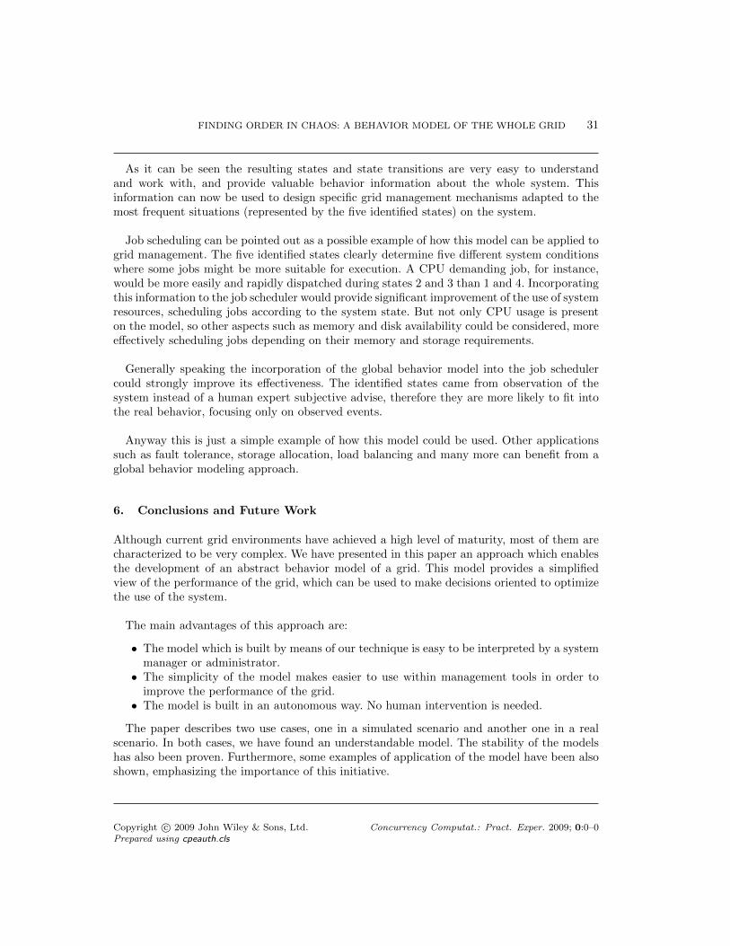
As it can be seen the resulting states and state transitions are very easy to understandand work with, and provide valuable behavior information about the whole system. Thisinformation can now be used to design specific grid management mechanisms adapted to themost frequent situations (represented by the five identified states) on the system.

Job scheduling can be pointed out as a possible example of how this model can be applied togrid management. The five identified states clearly determine five different system conditionswhere some jobs might be more suitable for execution. A CPU demanding job, for instance,would be more easily and rapidly dispatched during states 2 and 3 than 1 and 4. Incorporatingthis information to the job scheduler would provide significant improvement of the use of systemresources, scheduling jobs according to the system state. But not only CPU usage is presenton the model, so other aspects such as memory and disk availability could be considered, moreeffectively scheduling jobs depending on their memory and storage requirements.

Generally speaking the incorporation of the global behavior model into the job schedulercould strongly improve its effectiveness. The identified states came from observation of thesystem instead of a human expert subjective advise, therefore they are more likely to fit intothe real behavior, focusing only on observed events.

Anyway this is just a simple example of how this model could be used. Other applicationssuch as fault tolerance, storage allocation, load balancing and many more can benefit from aglobal behavior modeling approach.

6. Conclusions and Future Work

Although current grid environments have achieved a high level of maturity, most of them arecharacterized to be very complex. We have presented in this paper an approach which enablesthe development of an abstract behavior model of a grid. This model provides a simplifiedview of the performance of the grid, which can be used to make decisions oriented to optimizethe use of the system.

The main advantages of this approach are:

• The model which is built by means of our technique is easy to be interpreted by a systemmanager or administrator.

• The simplicity of the model makes easier to use within management tools in order toimprove the performance of the grid.

• The model is built in an autonomous way. No human intervention is needed.

The paper describes two use cases, one in a simulated scenario and another one in a realscenario. In both cases, we have found an understandable model. The stability of the modelshas also been proven. Furthermore, some examples of application of the model have been alsoshown, emphasizing the importance of this initiative.


32 J. MONTES ET AL.

As current and future work, we are trying to improve the generated model’s accuracy andabove all extending our approach to be able to predict the environment beahavior. By meansof this prediction it would be possible to anticipate events within the system and make moreaccurate decisions aimed at enhancing the global performance of the grid.

REFERENCES

1. I. Borg and J. Lingoes, Multidimensional similarity structure analysis. Springer-Verlag, 1987.2. Carmen Bratosin, Wil M. P. van der Aalst, Natalia Sidorova, and Nikola Trcka. A reference model for

grid architectures and its analysis. In Robert Meersman and Zahir Tari, editors, OTM Conferences (1),volume 5331 of Lecture Notes in Computer Science, pages 898–913. Springer, 2008.

3. R. Buyya, D. Abramson, and J. Giddy. Nimrod/g: an architecture for a resource management andscheduling system in a global computational grid. volume 1, pages 283–289 vol.1, 2000.

4. Rajkumar Buyya and Manzur Murshed. GridSim: A Toolkit for the Modeling and Simulation ofDistributed Resource Management and Scheduling for Grid Computing. Concurrency and Computation:Practice and Experience, 14(13–15):1175–1220, 2002.

5. John Carroll and Darrell Long. Theory of finite automata with an introduction to formal languages.Prentice-Hall, Inc., Upper Saddle River, NJ, USA, 1989.

6. J. L. Chandon and S. Pinson. Analyse typologique. Theorie et applications. Masson, Paris, 1981.7. CoMon - A Monitoring Infrastructure for PlanetLab, accessed Mar 2009 [Online]. Available:

http://comon.cs.princeton.edu/.8. Roy D’Andrade. U-statistic hierarchical clustering. Psychometrika, 43(1):59–67, March 1978.9. A. P. Dempster, N. M. Laird, and D. B. Rubin. Maximum likelihood from incomplete data via the em

algorithm. Journal of the Royal Statistical Society. Series B (Methodological), 39(1):1–38, 1977.10. Marios D. Dikaiakos. Grid benchmarking: vision, challenges, and current status: Research articles.

Concurr. Comput. : Pract. Exper., 19(1):89–105, 2007.11. Jack J. Dongarra and Wolfgang Gentzsch, editors. Computer benchmarks. Elsevier Science Publishers

B. V., Amsterdam, The Netherlands, The Netherlands, 1993.12. EGEE Portal: Enabling Grids for E-sciencE, accessed Mar 2009 [Online]. Available: http://www.eu-

egee.org/.13. Martin Ester, Hans-Peter Kriegel, S. Jorg, and Xiaowei Xu. A density-based algorithm for discovering

clusters in large spatial databases with noise, 1996.14. CERN European Organization for Nuclear Research. EGEE - Alice Job Summary, accessed Feb 2009

[Online]. Available: http://dashb-alice.cern.ch/dashboard/request.py/jobsummary.15. CERN European Organization for Nuclear Research. EGEE - Atlas Dashboard, accessed Dec 2008

[Online]. Available: http://dashb-atlas-prodsys-test.cern.ch/dashboard/request.py/summary.16. CERN European Organization for Nuclear Research. EGEE - Atlas Job Summary, accessed Feb 2009

[Online]. Available: http://dashb-atlas-job.cern.ch/dashboard/request.py/jobsummary.17. CERN European Organization for Nuclear Research. EGEE - CMS Job Summary, accessed Feb 2009

[Online]. Available: http://lxarda09.cern.ch/dashboard/request.py/jobsummary.18. I. Foster. What is the Grid? A Three Point Checklist. Grid Today, 1(6), Jul 2002.19. I. Foster and C. Kesselman, editors. The Grid 2: Blueprint for a New Computing Infrastructure. Morgan

Kaufmann Publishers, 2004.20. E. B. Fowlkes and C. L. Mallows. A method for comparing two hierarchical clusterings. Journal of the

American Statistical Association, 78(383):553–584, 1983.21. M. Frumkin and R. F. Van der Wijngaart. NAS Grid Benchmarks: A Tool for Grid Space Exploration.

Cluster Computing, 5(3):247–255, 2002.22. Ganglia distributed monitoring and execution system, accessed Mar 2009 [Online]. Available:

http://ganglia.info/.23. Yuri Gurevich. Evolving Algebras: An Attempt to Discover Semantics. In EATCS Bulletin, volume 43,

pages 264–284. European Assoc. for Theor. Computer Science, February 1991.24. Jiawei Han and Micheline Kamber. Data Mining: Concepts and Techniques (The Morgan Kaufmann

Series in Data Management Systems). Morgan Kaufmann, September 2000.25. S. Haykin. Neural Networks: A Comprehensive Foundation. Macmillan, New York, 1994.



26. Laurie J. Heyer, Semyon Kruglyak, and Shibu Yooseph. Exploring expression data: Identification andanalysis of coexpressed genes. Genome Res., 9(11):1106–1115, November 1999.

27. John E. Hopcroft, Rajeev Motwani, and Jeffrey D. Ullman. Introduction to Automata Theory, Languages,and Computation. Addison Wesley, 2nd edition, November 2000.

28. A. K. Jain and J. Mao, “Artificial neural networks for nonlinear projection of multivariate data,” 1992IEEE joint Conf. on Neural Networks, pp. 335–340, Baltimore, MD, 1992.

29. Stephen Johnson. Hierarchical clustering schemes. Psychometrika, 32(3):241–254, September 1967.30. J. O. Kephart and D. M. Chess. The vision of autonomic computing. Computer, 36(1):41–50, 2003.31. Klaus Krauter, Rajkumar Buyya, and Muthucumaru Maheswaran. A taxonomy and survey of grid

resource management systems for distributed computing. Software Practice and Experience, 32(2):135–164, 2002.

32. J. Kruskal, “Multidimensional scaling by optimizing goodness of fit to a nonmetric hypothesis,”Psichometrika, vol. 29 pp.1–27, 1964.

33. J. B. MacQueen. Some methods for classification and analysis of multivariate observations. In L. M. LeCam and J. Neyman, editors, Proc. of the fifth Berkeley Symposium on Mathematical Statistics andProbability, volume 1, pages 281–297. University of California Press, 1967.

34. GMonE: Grid Monitoring Environment, accessed Mar 2009 [Online]. Available:http://laurel.datsi.fi.upm.es/proyectos/globem/gmone/.

35. MonALISA - Monitoring the Grid since 2001, accessed Mar 2009 [Online]. Available:http://monalisa.cacr.caltech.edu/.

36. Zsolt Nemeth and Vaidy Sunderam. Characterizing grids: Attributes, definitions, and formalisms. Journalof Grid Computing, 1(1):9–23.

37. Zsolt N. Nemeth and Vaidy Sunderam. A formal framework for defining grid systems. In CCGRID ’02:Proceedings of the 2nd IEEE/ACM International Symposium on Cluster Computing and the Grid, page202, Washington, DC, USA, 2002. IEEE Computer Society.

38. H. B. Newman, I C Legrand, P Galvez, R Voicu, and C Cirstoiu. MonALISA : A Distributed MonitoringService Architecture. In 2003 Computing in High Energy and Nuclear Physics (CHEP03), La Jolla,California, USA, March 2003.

39. H. B. Newman, I.C. Legrand, and J.J. Bunn. A Distributed Agent-based Architecture for DynamicServices. In CHEP 2001, Beijing, September 2001.

40. Network Weather Service: Introduction, accessed Mar 2009 [Online]. Available:http://nws.cs.ucsb.edu/ewiki/.

41. Noam Palatin, Arie Leizarowitz, Assaf Schuster, and Ran Wolff. Mining for misconfigured machines in gridsystems. In KDD ’06: Proceedings of the 12th ACM SIGKDD international conferen ce on Knowledgediscovery and data mining, pages 687–692, New York, NY, USA, 2006. ACM.

42. Planetlab - An open platform for developing, deploying and accessing planetary-scale services, accessedMar 2009 [Online]. Available: http://www.planet-lab.org/.

43. Ross J. Quinlan. C4.5: Programs for Machine Learning (Morgan Kaufmann Series in Machine Learning).Morgan Kaufmann, January 1993.

44. William M. Rand. Objective criteria for the evaluation of clustering methods. Journal of the AmericanStatistical Association, 66(336):846–850, 1971.

45. J. W. Sammon, “A non-linear mapping for data structure analysis,” IEEE Trans. Computers, C18 pp.401–408, 1969.

46. A. Sanchez. Autonomic high performance storage for grid environments based on long term prediction.PhD thesis, Universidad Politecnica de Madrid, 2008.

47. J. M. Schopf, M. D’Arcy, N. Miller, L. Pearlman, I. Foster, and C. Kesselman. Monitoring and Discoveryin a Web Services Framework: Functionality and Performance of the Globus Toolkit’s MDS4. TechnicalReport ANL/MCS-P1248-0405, Argonne National Laboratory, April 2005.

48. Mumtaz Siddiqui and Thomas Fahringer. GridARM: Askalon’s Grid Resource Management System. InAdvances in Grid Computing - EGC 2005 - Revised Selected Papers, volume 3470 of Lecture Notes inComputer Science, pages 122–131, Amsterdam, Netherlands, June 2005. Springer Verlag GmbH, ISBN3-540-26918-5.

49. George Tsouloupas and Marios D. Dikaiakos. Gridbench: A tool for the interactive performanceexploration of grid infrastructures. J. Parallel Distrib. Comput., 67(9):1029–1045, 2007.

50. J. J. Valdes, “Virtual reality representation of relational systems and decision rules,” In P. Hajek, editor,Theory and Application of Relational Structures as Knowledge Instruments, Meeting of the COST Action274. Prague, Nov 2002.


34 J. MONTES ET AL.

51. J. J. Valdes, “Similarity-based heterogeneous neurons in the context of general observational models,”Neural Network World, vol. 12(5) pp. 499–508, 2002.

52. J. J. Valdes, “Virtual reality representation of information systems and decision rules,” Lecture Notes inArtificial Intelligence, vol. 2639 LNAI, pp. 615–618. Springer-Verlag, 2003.

53. J. Valdes, “Building virtual reality spaces for visual data mining with hybrid evolutionary-classicaloptimization: Application to microarray gene expression data,” 2004 IASTED International JointConference on Artificial Intelligence and Soft Computing, ASC’2004, pp. 161–166, Marbella, Spain, Sept2004. ACTA Press, Anaheim, USA.

54. J. J. Valdes, A.J. Barton, “Virtual Reality Visual Data Mining with Nonlinear Discriminant NeuralNetworks: Application to Leukemia and Alzheimer Gene Expression Data,” Proceedings of the IJCNN’05International Joint Conference on Neural Networks. July 31-August 4, 2005, Montreal, Canada

55. Rich Wolski. Experiences with predicting resource performance on-line in computational grid settings.SIGMETRICS Perform. Eval. Rev., 30(4):41–49, 2003.

56. Rich Wolski, Neil T. Spring, and Jim Hayes. The network weather service: a distributed resourceperformance forecasting service for metacomputing. Future Generation Computer Systems, 15(5–6):757–768, 1999.


finding order in chaos: a behavior model of the whole grid

Documents