finding minima in complex landscapes: annealed ... - arxiv · pdf filethe study of optimizing...
TRANSCRIPT

arX
iv:m
ath-
ph/0
4070
78v1
30
Jul 2
004
Finding Minima in Complex Landscapes:
Annealed, Greedy and Reluctant Algorithms
Pierluigi Contuccia, Cristian Giardinaa,Claudio Gibertib and Cecilia Verniac
a Dipartimento di Matematica, Universita di Bologna
Piazza di Porta S.Donato 5, 40127 Bologna, Italy
[email protected], [email protected]
b Dipartimento di Informatica e Comunicazione, Universita dell’Insubria,
via Mazzini 5, 21100 Varese, Italy
c Dipartimento di Matematica Pura ed Applicata, Universita di Modena
e Reggio Emilia, via Campi 213/B, 41100 Modena, Italy
April 5, 2017
Abstract
We consider optimization problems for complex systems in whichthe cost function has a multivalleyed landscape. We introduce a newclass of dynamical algorithms which, using a suitable annealing pro-cedure coupled with a balanced greedy-reluctant strategy drive thesystems towards the deepest minimum of the cost function. Resultsare presented for the Sherrington-Kirkpatrick model of spin-glasses.
1
1 Introduction.
There is a standard barrier in applied science: the computational complexityof hard (non-polynomial) problems. The modelling of competing interac-tions among the components of a large system often lead to consider thesolution of a problem as the minimum of a functional with a complex land-scape. The extensive search for the optimal configurations has a cost thatgrows too quickly (usually exponentially) and become practically intractablewhen the number of composing units is of the order of a few hundreds asin the interesting cases. The study of optimizing algorithms is then a basicstep toward the solution of specific practical problems emerging in differentfields of applied science. In this paper we build a strategy to efficientlyexplore the landscape of complex functionals in combinatorial optimizationin order to find its minima both local and global. To allow the reader tobetter focus on our method, let us describe the functional to be minimizedas the mathematical representation of a quickly changing mountain profile(in large dimensions), with a high multiplicity of local minima separatedby high barriers. The a priori knowledge of the landscape geometry is verypoor and our strategy to explore the territory in order to find good qualityminima (close to the global one) is to send signals in random directions (ini-tial configurations), follow their evolution according to a specified dynamics(algorithm) and collect the observed results. Our investigation procedureis not dissimilar from an optical instrument in which we may tune a fewparameters to better observe the landscape and find the sites which we areinterested in. The algorithm is preliminary set by choosing the elementarydynamical moves: this choice reflects the topology that we are associatingto our landscape and comes with a notion of vicinity and nearest neigh-boring sites. The successive step is to decide the criteria after which toselect among a large multiplicity of moves. This is done by keeping intoaccount what we search for and what we most fear: we want to reach thebest possible minima as quickly as possible and the worse happening is toget stuck in a local minimum which is still far from the optimal or near op-timal ones. It appears rather intuitive that an algorithm with a too steepydescent (greedy) has a very high risk to get stuck in poor local minima, butat the same time a too slow descent (reluctant) would cost a very high pricein terms of computer time. It is natural to expect, and indeed it is what wefind, an optimal speed of descent that compromise at best among havinga wide exploration basin in a reasonable amount of time. Yet the dangerof remaining caught in wrong local minima remains. To avoid it we alsoallow moves which locally and momentarily deviates from the descending
2

directions. In other terms: to reach a good minimum it is often necessaryto overcome a high barrier. Physically, the introduction of a similar possi-bility works like the availability of thermal energy where the probability ofits happening is related to the temperature of the system: the higher thetemperature the more likely are moves upwards and viceversa. To introducesuch a useful strategy we initially allow upward and downward moves; withthe time passing the probability to go up is progressively decreased at arate which we may optimize (this simulates the annealing of a physical sys-tem) and the algorithm will continue evolving according to its downwardmoves. Our work and the implementation of the algorithm is built andtested toward a standard model in combinatorial optimization with originsin condensed matter physics: the Sherrington-Kirkpatrick (SK) model forthe mean field spin glass phase [1, 2]. Among the advantages of our ap-proach, there is the flexibility of our algorithms and their wide applicabilityto practical problems like protein folding in biology [2], portfolio optimiza-tion in financial mathematics [3], error correcting codes for digital signaltransmissions [4].
2 Results.
In the following Sections we will present details of the Model and Algorithmswe used in our simulations. Here we summarize the main ideas and resultsof our analysis.
In the Sherrington-Kirkpatrick model the cost function is identified withthe energy of the system, the domain of the cost function is the discretespin configuration space and the optimization problem amounts to find thespin configuration with the lowest energy (ground state). Given a properdefinition of distance in the configuration space (we can think two spin con-figurations to be close if they differ only for a single spin-flip), the energy ofthe system is a real-valued function forming a complex and corrugated en-ergy landscape, with valleys (local minima) and peaks (local maxima). Ouroptimization algorithms are described as dynamical evolution rules in thisenergy landscape which, starting from a random initial condition, drive thesystem towards local minima of the energy. The random transition from apoint of the trajectory to the successive, which is a nearest neighboring one,is ruled by a probability with exponential density. We consider four differ-ent algorithms: starting from the simplest one (Algorithm 0) which allowsonly energy-decreasing trajectories, we implement a sequence of refinements(Algorithms 1,2,3) leading to more efficient strategies, which exploit also in-
3

creases in the cost function.
With Algorithm 0 the cost-decreasing trajectory ends up as soon as itreaches a configuration which, according to our notion of vicinity (see Sec. 3)is a local minimum. The parameter controlling the transition probabilityfunction tunes the steepness of descents, generating a continuum of behav-iors ranging from a reluctant-type dynamics (very small jumps and slowconvergence) to a greedy-type one (very large jumps deep into a valley).
A first improvement of this strategy, implemented in Algorithms 1 and 2, isobtained by introducing a “temperature” in the system, which enables ran-dom positive fluctuations of the cost function. This is obtained through thechoice of a transition probability which gives a non zero weight to upwardsmoves. With these choices we have the following scenario for Algorithms1 and 2: the dynamics starts with a given initial temperature and equalprobability of positive and negative moves. As the time goes on, the systemis gradually cooled until it reaches a state in which positive fluctuations areforbidden and the dynamics continues as either greedy or reluctant, depend-ing on the initial temperature. With a high initial temperature the long termbehavior of the dynamics will be greedy-like, while a low initial temperaturewill lead to reluctant-type motion. The difference between Algorithm 1 and2 lies in the convergence criterium: while the former stops when the firstlocal minimum is attained (likewise Algorithm 0), the latter allows the tra-jectory to escape from it in view of the possibility to reach deeper minima(supplementary stopping conditions are required in this case).
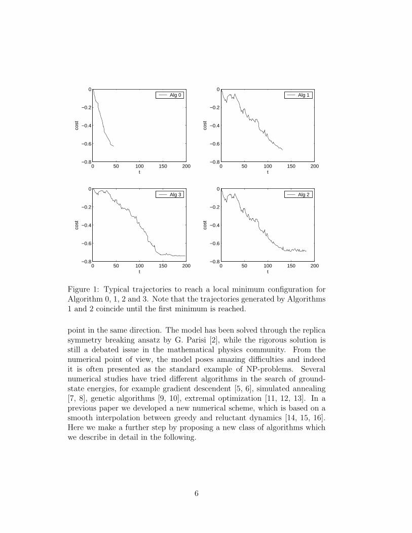
A further improvement of the algorithm efficiency is obtained with Algo-rithm 3. In this case, the transition probability is designed to model aninitially hot system with high probability of positive moves, which is gradu-ally quenched; when the system is cool, positive fluctuations are absent andthe decreasing trajectories are forced to follow greedy-like paths. In Fig. 1typical trajectories for the four different algorithms are reported.
The efficiency of the algorithms are quantified on one hand by measuringthe average time needed to reach a local minimum, on the other hand by thequality of the found minima (i.e. how deep they are). The optimization isdone by tuning the parameters which control the transition probabilities; inparticular, for Algorithms 1 and 2 this parameter is mainly the initial tem-perature, while for Algorithm 3 it is the rate of the quench, i.e. the speedof convergence to zero of the temperature of the system. As one would ex-pect, for low initial temperatures (very low possibility of energy increase),Algorithm 1 and 2 behaves very much as Algorithm 0. However their differ-
4
ences become effective for sufficiently high initial temperatures. Obviously,allowing positive jumps and escapes from local minima, the relaxation timesincrease passing from Algorithm 0 to Algorithm 2; less trivially, numericalresults show that the scaling of the execution times with respect to the sys-tem size is greatly enhanced. This is an important fact, because it suggeststhat a crossover between computation times is to be expected for systemswith larger sizes. As regards the lowest values found, similar conclusionscan be drawn: going from Algorithm 0 to Algorithm 2 deeper minima areattained.
Algorithm 3 can be consistently compared with Algorithm 2, which is thebest performing among the first three. The computation times and theirscaling with the size are similar for the two algorithms when the initial tem-perature (for Algorithm 2) is high, but a clear enhancement is obtained byAlgorithm 3 when it is low. Also the minimal values of the cost functionalare similar for high temperatures, while they are lower for Algorithm 2 withlow initial temperatures. The previous remarks refer to an experimentalprotocol in which the search for low cost configurations is performed testinga fixed number of trajectories. The minimization of cost at fixed elapsedcomputer time is another relevant criterium for the comparison of the al-gorithms. In this case the best result is obtained with Algorithm 3, eventhough Algorithm 2 gives comparable results.
3 The model and the algorithms.
3.1 The Sherrington Kirkpatrick model
The system we study is the Sherrington-Kirkpatrick model of spin-glasses[1]. It is defined by the Hamiltonian
H(J, σ) = − 1√N
∑
1≤i<j≤N
Jijσiσj (1)
where σi = ±1 for i = 1, . . . , N are Ising spin variables which interactthrough couplings Jij . These are gaussian random variables, independentand identically distributed with zero mean and variance 1. The randomsign (and strength) of the interaction generates frustration in the system,i.e. the fact that in low energy configurations some of the couples will haveunsatisfied interaction. In particular, the ground state of the system is farfrom the standard ground state of ferromagnetic models, where all spins
5
0 50 100 150 200−0.8
−0.6
−0.4
−0.2
0
t
cost
Alg 0
0 50 100 150 200−0.8
−0.6
−0.4
−0.2
0
t
cost
Alg 1
0 50 100 150 200−0.8
−0.6
−0.4
−0.2
0
t
cost
Alg 3
0 50 100 150 200−0.8
−0.6
−0.4
−0.2
0
t
cost
Alg 2
Figure 1: Typical trajectories to reach a local minimum configuration forAlgorithm 0, 1, 2 and 3. Note that the trajectories generated by Algorithms1 and 2 coincide until the first minimum is reached.
point in the same direction. The model has been solved through the replicasymmetry breaking ansatz by G. Parisi [2], while the rigorous solution isstill a debated issue in the mathematical physics community. From thenumerical point of view, the model poses amazing difficulties and indeedit is often presented as the standard example of NP-problems. Severalnumerical studies have tried different algorithms in the search of ground-state energies, for example gradient descendent [5, 6], simulated annealing[7, 8], genetic algorithms [9, 10], extremal optimization [11, 12, 13]. In aprevious paper we developed a new numerical scheme, which is based on asmooth interpolation between greedy and reluctant dynamics [14, 15, 16].Here we make a further step by proposing a new class of algorithms whichwe describe in detail in the following.
6
3.2 Dynamical Algorithms
We focus our attention on stochastic dynamics that generates a sequenceof spin configurations ending up on a local energy minimum. The smoothinterpolation between greedy and reluctant dynamics studied in a previouswork [16] follows an energy-decreasing trajectory and terminates in the firstlocal minimum it encounters: only transitions corresponding to a decreasein the cost (energy) function are allowed by the algorithm. In the samespirit of Simulated Annealing strategies [7], where a slow decrease of thetemperature leads the system through successive metastable states withlower and lower energy, we think of a class of algorithms which also accept,in some limited way, transitions corresponding to an increase in the costfunction. In fact, these algorithms are based on the statistical propertiesof metastable states: they are organized with some structure so that theevolution dynamics can be considered as the overlapping of a “fast” motionin the basin of attraction of a local minimum and of a “slow” motion withjumps between minima (the time of the dynamics is determined by theenergy barriers between these metastable states).
In the algorithms that we are going to introduce, the transition between thespin configuration at time t, σ(t) = (σ1(t), . . . , σN(t)), and the successiveconfigurations at time t + 1, σ(t + 1) = (σ1(t + 1), . . . , σN(t + 1)) dependson the spectrum of energy changes of σ(t), obtained by flipping the spin inposition i, for i = 1, . . . , N :
∆Ei = σi(t)∑
j 6=i
Jijσj(t). (2)
Let also define ∆Ei = min1≤i≤N ∆Ei that will be used in what follows. As
a first step, let us briefly recall the algorithm studied in [16], where onlyenergy decreasing trajectory are considered. It is described by the followingprocedure:
Algorithm 0
1. Initialization: choose an initial spin configuration σ(0) and a param-eter value for λ > 0.
2. Generate a random number D with probability density
f(x) =
{
λeλx if x ≤ 00 if x > 0
(3)
7
3. Select the site i⋆ associated with the closest energy change to the valueD, i.e.:
i⋆ : |∆Ei⋆ −D| = mini∈{1,...,N}
{|∆Ei −D| : ∆Ei < 0}. (4)
4. Flip the spin on site i⋆:
σi(t + 1) =
{
−σi(t) if i = i⋆
σi(t) if i 6= i⋆.(5)
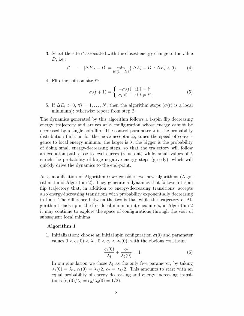
5. If ∆Ei > 0, ∀i = 1, . . . , N , then the algorithm stops (σ(t) is a localminimum); otherwise repeat from step 2.
The dynamics generated by this algorithm follows a 1-spin flip decreasingenergy trajectory and arrives at a configuration whose energy cannot bedecreased by a single spin-flip. The control parameter λ in the probabilitydistribution function for the move acceptance, tunes the speed of conver-gence to local energy minima: the larger is λ, the bigger is the probabilityof doing small energy-decreasing steps, so that the trajectory will followan evolution path close to level curves (reluctant) while, small values of λenrich the probability of large negative energy steps (greedy), which willquickly drive the dynamics to the end-point.
As a modification of Algorithm 0 we consider two new algorithms (Algo-rithm 1 and Algorithm 2). They generate a dynamics that follows a 1-spinflip trajectory that, in addition to energy-decreasing transitions, acceptsalso energy-increasing transitions with probability exponentially decreasingin time. The difference between the two is that while the trajectory of Al-gorithm 1 ends up in the first local minimum it encounters, in Algorithm 2it may continue to explore the space of configurations through the visit ofsubsequent local minima.
Algorithm 1
1. Initialization: choose an initial spin configuration σ(0) and parametervalues 0 < c1(0) < λ1, 0 < c2 < λ2(0), with the obvious constraint
c1(0)
λ1
+c2
λ2(0)= 1 (6)
In our simulation we chose λ1 as the only free parameter, by takingλ2(0) = λ1, c1(0) = λ1/2, c2 = λ1/2. This amounts to start with anequal probability of energy decreasing and energy increasing transi-tions (c1(0)/λ1 = c2/λ2(0) = 1/2).
8
2. Generate a random number D with probability function
ft(x) =
{
c1(t)eλ1x if x ≤ 0
c2e−λ2(t)x if x > 0
(7)
3. Select the site i⋆ associated with the closest energy change to the valueD and with the same sign, i.e.:
i⋆ : |∆Ei⋆ −D| = mini∈{1,...,N}
{|∆Ei −D| : ∆Ei ·D > 0}. (8)
4. Flip the spin on site i⋆:
σi(t + 1) =
{
−σi(t) if i = i⋆
σi(t) if i 6= i⋆.(9)
5. If ∆Ei > 0, ∀i = 1, . . . , N , then the algorithm stops (σ(t) is a localminimum). Otherwise, change the parameter λ2(t) of the probabilitydistribution in step 2 with a suitable scheduling, for example
λ2(t) =λ2(0)
kt, 0 < k < 1 (10)
and return to step 2.
The trajectory generated by Algorithm 1 wonder in the energy landscape(by a succession of moves which decrease and increase energy) till it arrivesto a local minimum. Starting from a symmetric probability distribution forthe spin-flip selection, as time goes on the probability of energy-increasingmoves is decreased by the update rule (10).
Next, we want to consider an algorithm as the previous one but with thepossibility of exploring subsequent minima. The problem one has to solveis to give an efficient criterium to stop the dynamics. We considered thefollowing implementation:
Algorithm 2
1. Initialization: as in Algorithm 1. Set also m = 1000 and ǫ = 10−4.
2. Generate a random number D as follows:
with probability function
ft(x) =
{
c1(t)eλ1x if x ≤ 0
c2e−λ2(t)x if x > 0
ifc1(t)
λ1
≤ mc2
λ2(t)(11)
9

and with probability function
f(x) =
{
λ1eλ1x if x ≤ 0
0 if x > 0if
c1(t)
λ1> m
c2λ2(t)
(12)
3. Select the site i⋆ associated with the closest energy change to the valueD and with the same sign, i.e.:
i⋆ : |∆Ei⋆ −D| = mini∈{1,...,N}
{|∆Ei −D| : ∆Ei ·D > 0}. (13)
4. Flip the spin on site i⋆:
σi(t + 1) =
{
−σi(t) if i = i⋆
σi(t) if i 6= i⋆.(14)
5. If ∆Ei > 0, ∀i = 1, . . . , N , and Pt(D ≥ ∆Ei) < ǫ then Stop.
D is a random number, Pt is the cumulative function of the probabilitydescribed in step 2 and ǫ is a small parameter. In other words, ifwe arrive in a minimum and the probability of a significant energyincreasing transition from this local minimum is too small (or evenzero when the energy increases are forbidden, see step 2), then thealgorithm stops.
6. Change the probability distribution (11) with the scheduling (10) forλ2(t) (the same scheduling used in Algorithm 1) and return to step 2.
As in Algorithm 1, the dynamics generated by this algorithm follows a 1-spin flip trajectory making a combination of upwards and downwards moves.However, in this case, the trajectory does not end up in the first 1-spin flipstable configuration it encounters, at least as long as the probability ofpositive moves (c2/λ2(t)) remains greater than a certain threshold (1/mtimes the probability of negative moves c1(t)/λ1 - in our experiments m =1000). With this strategy it is possible to escape from the local minima toexplore the neighboring space in view of (possible) lower energy minima.When the probability of energy increases exceed this fixed threshold, fromthis point on, only decreases in energy are accepted and so the processterminates when the subsequent local minimum is reached. In fact, whenthe process starts at time t = 0 we choose equal probabilities c1(0)/λ1 andc2/λ2(0) of cost-decreasing or cost-increasing moves, respectively, by settlingc2 = λ2(0)/2. As the algorithm continues its execution, we decrease c2/λ2(t)
10

towards zero, varying the control parameter λ2(t) in accordance with theabove mentioned law (10):
λ2(t) =λ2(0)
kt, λ2(0) = λ1, 0 < k < 1
(and keeping fixed λ1) untilc1(t)λ1
≤ m c2λ2(t)
; as a consequence, the probability
of energy-decreasing move acceptance c1(t)/λ1 tends to one (c1(t) = λ1(1−c2/λ2(t))). Therefore, while the speed of convergence to the local energyminima is mainly tuned by λ1, the vanishing velocity of the probability ofenergy-increasing steps is governed by the parameter k. Of course, large λ1
(and λ2(t)) lead to evolution paths generated by small (in absolute value)energy changes (annealed reluctant dynamics) and the closer k is to 1, theslower λ2(t) grows and then the more energy increases are enabled. Whenc1(t)λ1
> m c2λ2(t)
the dynamics continues governed only by the parameter λ1,not depending on t.
We see that for Algorithm 2 the possibility to escape from the minima iseffective only when λ1 is sufficiently small (say λ1 ≃ 1, and then λ2(0) ≃ 1,see (10)). For greater values of λ1 the possibility to explore successiveminima is not exploited and both the dynamics 1 and 2 can be expectedto give similar results in terms of achieved minimum energy level. In thesecases, the dynamics generated by Algorithm 2 ends up naturally, after t′
steps, in the first minimum it encounters, because the (step dependent)probability Pt′ to escape from this configuration is too small; therefore, weexpect that for large values of λ1 Algorithms 1 and 2 should be equivalent.
Since for these algorithms the speed of convergence to the finale state isgoverned by the probability function ft(x), we can consider a third algorithmin which the time dependence is present only in the control parameters λi(t),i = 1, 2; in this case, starting from a (in general) non symmetric probabilityfunction, the dynamics evolves gradually towards a final scenario in whichthe system is cooled by tuning the control parameter λ1(t).
Algorithm 3
1. Initialization: choose an initial spin configuration σ(0) and parametervalues λ1(0), λ2(0) such that 1/λ1(0)+1/λ2(0) = 1. Set also m = 1000and ǫ = 10−4.
2. Generate a random number D as follows:
11
with probability function
ft(x) =
{
eλ1(t)x if x ≤ 0e−λ2(t)x if x > 0
if1
λ1(t)≤ m
1
λ2(t)(15)
and with probability function
f(x) =
{
λ1eλ1x if x ≤ 0
0 if x > 0if
1
λ1(t)> m
1
λ2(t)(16)
3. Select the site i⋆ associated with the closest energy change to the valueD and with the same sign, i.e.:
i⋆ : |∆Ei⋆ −D| = mini∈{1,...,N}
{|∆Ei −D| : ∆Ei ·D > 0}. (17)
4. Flip the spin on site i⋆:
σi(t + 1) =
{
−σi(t) if i = i⋆
σi(t) if i 6= i⋆.(18)
5. If ∆Ei > 0, ∀i = 1, . . . , N , and Pt(D ≥ ∆Ei) < ǫ then Stop (as inAlgorithm 2) .
6. Change the probability distribution defined in (15) with the samescheduling for λ2(t) used in Algorithm 2 and return to Step 2.
The main difference between Algorithm 2 and Algorithm 3 is that in thelatter, when the process starts at time t = 0 we have (if λ1(0) 6= 2) dif-ferent probabilities of energy-decreasing moves (1/λ1(0)) and of energy-increasing moves (1/λ2(0)). As Algorithm 3 continues its execution, wedecrease 1/λ2(t) towards zero, varying the control parameter λ2(t) in accor-dance with the scheduling:
λ2(t) =λ2(0)
kt, λ2(0) =
λ1(0)
λ1(0)− 1, 0 < k < 1 (19)
until 1λ1(t)
≤ m 1λ2(t)
; as a consequence, the probability of energy-decreasing
move acceptance 1/λ1(t) tends to one (λ1(t) =λ2(t)
λ2(t)−1). Therefore, while the
speed of convergence to the final state is mainly tuned by the initial valueλ1(0) of the time dependent parameter λ1(t) (which tends to 1, as timet increases), the vanishing velocity of the probability of energy-increasingsteps is governed by the parameter k. When 1
λ1(t∗)> m 1
λ2(t∗)the dynamics
12
−2 −1 0 1 20
0.2
0.4
0.6
0.8
1
1.2
1.4Alg 1 e 2, t=0
−2 −1 0 1 20
0.2
0.4
0.6
0.8
1
1.2
1.4Alg 3, t=0
(a) (b)
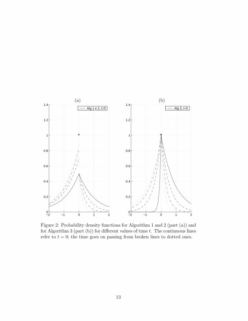
Figure 2: Probability density functions for Algorithm 1 and 2 (part (a)) andfor Algorithm 3 (part (b)) for different values of time t. The continuous linesrefer to t = 0; the time goes on passing from broken lines to dotted ones.
13
continues, for t > t∗, governed only by the parameter λ1 = λ1(t∗) (close to
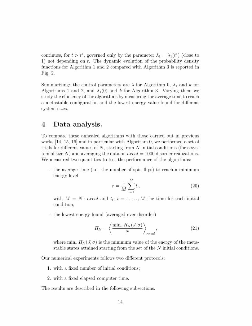
1) not depending on t. The dynamic evolution of the probability densityfunctions for Algorithm 1 and 2 compared with Algorithm 3 is reported inFig. 2.
Summarizing: the control parameters are λ for Algorithm 0, λ1 and k forAlgorithms 1 and 2, and λ1(0) and k for Algorithm 3. Varying them westudy the efficiency of the algorithms by measuring the average time to reacha metastable configuration and the lowest energy value found for differentsystem sizes.
4 Data analysis.
To compare these annealed algorithms with those carried out in previousworks [14, 15, 16] and in particular with Algorithm 0, we performed a set oftrials for different values of N , starting from N initial conditions (for a sys-tem of size N) and averaging the data on nreal = 1000 disorder realizations.We measured two quantities to test the performance of the algorithms:
- the average time (i.e. the number of spin flips) to reach a minimumenergy level
τ =1
M
M∑
i=1
ti, (20)
with M = N · nreal and ti, i = 1, . . . ,M the time for each initialcondition;
- the lowest energy found (averaged over disorder)
HN =
⟨
minσ HN(J, σ)
N
⟩
nreal
, (21)
where minσ HN(J, σ) is the minimum value of the energy of the meta-stable states attained starting from the set of the N initial conditions.
Our numerical experiments follows two different protocols:
1. with a fixed number of initial conditions;
2. with a fixed elapsed computer time.
The results are described in the following subsections.
14
10
100
1000
10000
10 100 1000
=1,k=.98=1,k=.99
=1,k=.995=10,k=.98=10,k=.99
=10,k=.995=100,k=.98=100,k=.99
=100,k=.995
N
τλ1
λ1
λ1
λ1
λ1
λ1
λ1
λ1
λ1
······························
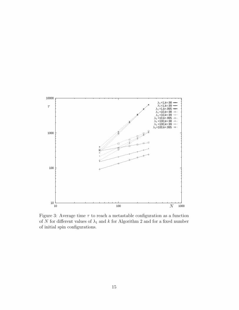
Figure 3: Average time τ to reach a metastable configuration as a functionof N for different values of λ1 and k for Algorithm 2 and for a fixed numberof initial spin configurations.
15

4.1 Fixed number of initial conditions
The dynamics of Algorithm 0 has been shown [16] to behave as a smoothinterpolation between greedy and reluctant dynamics [14] depending on theparameter λ: small λ (say λ ≃ 1) plays the role of the greedy algorithm,while large λ (say λ ≃ 100) that of reluctant. In fact, the relaxation timeτ(N) grows linearly with the system size when λ ≃ 1 and quadratically whenλ ≃ 100 (see Tab. 1), as it was previously observed in [14] for deterministicgreedy and reluctant regimes.
In Fig. 3, which refers to Algorithm 2, we represent τ as a function of N(N ∈ [25, 300]). We performed the analysis for different values of the controlparameters. For the sake of space, we show only the values λ1 = 1, 10, 100and three values of k (k = .98, .99, .995) for each λ1, together with the bestnumerical fits. Fig. 3 shows the progressive increase of the slope in log-logscale from a sub-linear law in N for λ1 = 1 and k = .98 ( ⋄—) to a super-linearone for λ1 = 100 and k = .98 ( ×· · ·). More in detail, the numerical fits ofτλ1,k(N) ∼ Na in Fig. 3 are reported in Tab.1.
Table 1: Numerical fits of τλ(N) ∼ Na for Algorithm 0 (with the symbolsof Fig. 6) and of τλ1,k(N) ∼ Na for Algorithm 1 and Algorithm 2 (with thesymbols of Fig. 3)
Alg 0 Alg 1 Alg 2λ a symbol λ1 k a λ1 k a symbol
.98 .687 .98 .549 ⋄—1 1.027 ∗ 1 .99 .630 1 .99 .475 +—
.995 .592 .995 .299 �—.98 1.041 .98 1.030 ⋄· · ·
10 1.263 10 .99 .948 10 .99 .891 +· · ·.995 .858 .995 .687 �· · ·.98 1.724 .98 1.771 ×· · ·
100 1.932 ⋄ 100 .99 1.591 100 .99 1.691 △· · ·.995 1.499 .995 1.567 ∗· · ·
With the same protocol (fixed number of initial conditions), we measuredthe lowest energy HN found by the algorithms. As a general remark werecall that from a theoretical point of view it is proved the monotonicity inN of the ground state energy (this follows from sub-additivity [17]). For thelargest size we have studied, some values of the simulation parameters give a
16

non-monotone behavior inN , suggesting that we are not actually finding thetrue lowest energy state. A larger number of trials (i.e. initial conditions)would be needed to achieve the global minimum. However, our principalaim here is not to have a perfect measure of ground state energies. In Fig. 4we represent, for Algorithm 2, HN as a function of N for different values ofλ1 and k. The best results for large N are obtained for λ1 = 100 and k = .98which corresponds to annealed reluctant dynamics (as found for Algorithm0, see Fig. 5). Therefore, this confirms [15, 16] that, for a fixed number ofinitial spin configurations, the algorithm that makes moves correspondingto the “smallest” possible energy change keeping the possibility of energyincrease only for the first steps of the algorithm is the most efficient inreaching low-energy states. Note that, for λ1 = 1 and k = .995 the attainedenergy values are sufficiently low: even if these results are not better thanthose for λ1 = 100 (with k = .98 and k = .995), they should not be
discarded since the average time scales better ( τ(2)1,.995(N) ∼ N .299 instead
of τ(2)100,.98(N) ∼ N1.771 or τ
(2)100,.995(N) ∼ N1.567) 1.
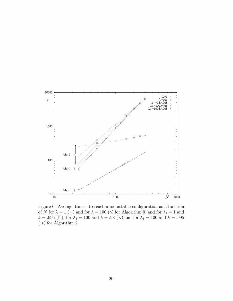
Comparing these results with those obtained with the interpolatinggreedy and reluctant algorithm (Algorithm 0) [16] we note (Figs. 5 and6 and Tab. 1) that for small λ and λ1 Algorithm 2 is better performing thanAlgorithm 0 both with respect to average time and energy levels, whilefor greater λ and λ1 we find comparable energy values but with lower costfor the computational time for Algorithm 2 (τ
(2)100,.98(N) ∼ N1.771 instead of
τ(0)100(N) ∼ N1.932).
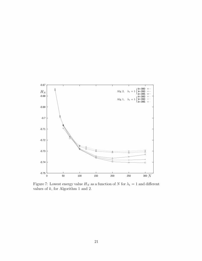
The same analysis is considered also for Algorithm 1. The comparisonbetween Algorithms 1 and 2 shows that the possibility of exceed the energybarriers between minima is useful only for small values of λ1 (for λ1 closeto 1 Algorithm 2 is more efficient than Algorithm 1 in reaching lower en-ergy states) while for λ1 ≥ 5 the performances of Algorithms 1 and 2 arepractically indistinguishable (see Figs. 7 and 8). Moreover, we note thatthe best scaling of the average time τλ1,k with respect to N is obtained with
Algorithm 2 (see Tab. 1), though for fixed N, λ1 and k, we have τ(1)λ1,k
< τ(2)λ1,k
.
Figures 9 and 10 report the results of the analysis of Algorithm 3 with afixed number of initial conditions: N ∈ [25, 400]) for three distinct valuesof λ1(0) (λ1(0) = 2, 10, 100) and for four values of k (k = .98, .99, .995, .997)for each λ1(0). Because of high computational costs (which increase withλ1(0) and k), the cases N = 350 and N = 400 for λ1(0) = 100 are onlypartially studied. For the same reason also the case k = .997 is considered
1From now on, the superscript (x) in the notation of the average time τ(x) will refer
to the number of the corresponding algorithm.
17

-0.745
-0.74
-0.735
-0.73
-0.725
-0.72
-0.715
-0.71
-0.705
0 50 100 150 200 250 300
=1,k=.98=1,k=.99
=1,k=.995=10,k=.98=10,k=.99
=10,k=.995=100,k=.98=100,k=.99
=100,k=.995
N
HN
λ1
λ1
λ1
λ1
λ1
λ1
λ1
λ1
λ1
Figure 4: Lowest energy value HN as a function of N for different values ofλ1 and k for Algorithm 2 and for a fixed number of initial conditions.
18

-0.75
-0.74
-0.73
-0.72
-0.71
-0.7
-0.69
-0.68
-0.67
0 50 100 150 200 250 300
=1=100
=1,k=.995=100,k=.98
N
HNλ
λλ1
λ1
Alg 0
{
Alg 2
{
Figure 5: Lowest energy value HN as a function of N obtained using aprotocol with a fixed number of initial conditions for λ = 1 (∗) and λ = 100(⋄) for Algorithm 0 and for λ1 = 1 and k = .995 (�) and for λ1 = 100 andk = .98 (×) for Algorithm 2.
19
10
100
1000
10000
10 100 1000
=1=100
=1,k=.995=100,k=.98
=100,k=.995
N
τλ
λλ1
λ1
λ1
Alg 2
Alg 0 {
Alg 0 {
Figure 6: Average time τ to reach a metastable configuration as a functionof N for λ = 1 (+) and for λ = 100 (⋄) for Algorithm 0, and for λ1 = 1 andk = .995 (�), for λ1 = 100 and k = .98 (×),and for λ1 = 100 and k = .995( ∗) for Algorithm 2.
20
-0.75
-0.74
-0.73
-0.72
-0.71
-0.7
-0.69
-0.68
-0.67
0 50 100 150 200 250 300
k=.980k=.990k=.995k=.980k=.990k=.995
N
HNAlg 2, λ1 = 1
{
.
Alg 1, λ1 = 1
{
.
Figure 7: Lowest energy valueHN as a function ofN for λ1 = 1 and differentvalues of k, for Algorithm 1 and 2.
21

-0.75
-0.74
-0.73
-0.72
-0.71
-0.7
-0.69
-0.68
-0.67
0 50 100 150 200 250 300
k=.980k=.990k=.995k=.980k=.990k=.995
N
HNAlg 2, λ1 = 10
{
.
Alg 1, λ1 = 10
{
.
Figure 8: Lowest energy value HN as a function of N for λ1 = 10 and fordifferent values of k obtained with Algorithm 1 and 2.
22

only for λ1(0) = 2.
Fig. 10 shows that Algorithm 3 seems to depend weakly on the parameterλ1(0), its behavior being mainly ruled by k. In fact, the lines of the HN
values corresponding to the same choices of k are grouped into narrow bandswell separated one from the others. Moreover, a closer look to Fig. 10 showsthat the best result for HN is obtained for λ1(0) = 2 and k = .997. Notethat for any λ1(0), the closer the values of k to one, the lower the valuesof energy: slow growths of the parameter λ2(t) enable energy increases andthen the possibility to exceed the energy barriers. Even though Algorithm2 is slightly better performing (λ1 = 100, k = .98 see Fig. 4) in terms ofminimum energy level reached, the best scaling of τλ1(0),k(N) is obtainedby Algorithm 3. In fact, for Algorithm 3 we note (Fig. 9 and Tab. 2)the progressive increase of the slope in log-log scale from a scaling lawτ(3)λ1(0),k
(N) ∼ N .22 for λ1(0) = 100 and k = .995 ( ∗· · ·) to τ(3)λ1(0),k
(N) ∼ N .53
for λ1(0) = 2 and k = .98 ( ⋄—). More in detail, the numerical fits ofτλ1(0),k(N) ∼ Na for Algorithm 3 are reported in Tab.2.
To conclude the analysis of the protocol with a fixed number of initialconditions we can say that taking into account also the average time τ , thebest performing algorithm in reaching minimum energy level is Algorithm 3(Fig. 11). In fact, Algorithm 3 with λ1(0) = 2 e k = .997 attains minimumenergy levels comparable with those obtained by the other algorithms withλ and λ1 equal to 100 but with lower computational costs (τ
(3)2,.997 ∼ N .272
while τ(0)100 ∼ N1.932, τ
(1)100,.98 ∼ N1.724 and τ
(2)100,.98 ∼ N1.771, see Tabs. 1 and
2).
4.2 Fixed elapsed computer time
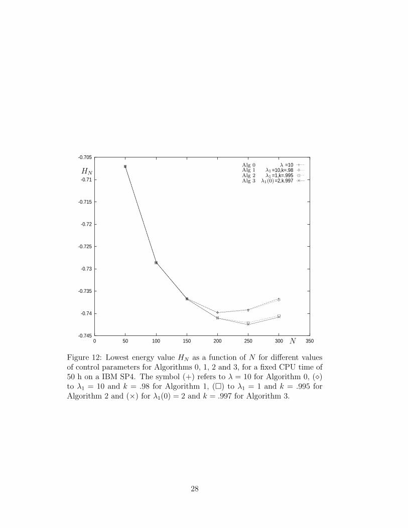
Finally, we analyze the lowest energy states found by the dynamics varyingthe control parameters for a given elapsed running time for all algorithms.In Fig. 12 we consider the minimum energy values HN , obtained by choosingdifferent system sizes N and, for each of them, different parameter values(λ = 1, 10, 100 for Algorithm 0, λ1 = 1, 5, 10, 100 for Algorithm 1, λ1 =1, 10 for Algorithm 2 and λ1(0) = 2, 10, 100 for Algorithm 3) with differentannealing scheduling each (k = .98 and k = .995 for Algorithm 1 and 2,k = .995 and k = .997 for Algorithm 3), for a fixed time of 50 h of CPU on aIBM SP4. For Algorithm 2 we consider in detail mainly the case (λ1 = 1) inwhich the dynamics behaves differently from that generated by Algorithm 1.Each run (i.e. for fixed N and for fixed control parameter) consists of 1000disorder realizations, with the same CPU time length (3 min.) assigned to
23
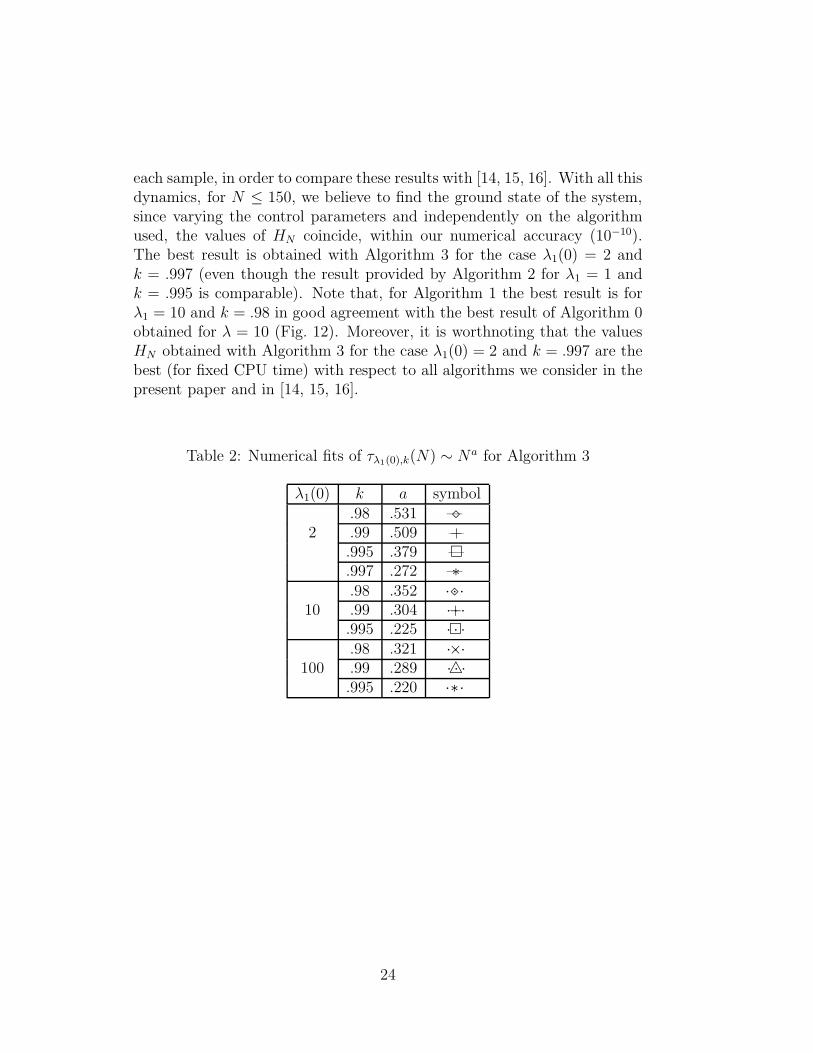
each sample, in order to compare these results with [14, 15, 16]. With all thisdynamics, for N ≤ 150, we believe to find the ground state of the system,since varying the control parameters and independently on the algorithmused, the values of HN coincide, within our numerical accuracy (10−10).The best result is obtained with Algorithm 3 for the case λ1(0) = 2 andk = .997 (even though the result provided by Algorithm 2 for λ1 = 1 andk = .995 is comparable). Note that, for Algorithm 1 the best result is forλ1 = 10 and k = .98 in good agreement with the best result of Algorithm 0obtained for λ = 10 (Fig. 12). Moreover, it is worthnoting that the valuesHN obtained with Algorithm 3 for the case λ1(0) = 2 and k = .997 are thebest (for fixed CPU time) with respect to all algorithms we consider in thepresent paper and in [14, 15, 16].
Table 2: Numerical fits of τλ1(0),k(N) ∼ Na for Algorithm 3
λ1(0) k a symbol.98 .531 ⋄—
2 .99 .509 +—.995 .379 �—.997 .272 ∗—.98 .352 ⋄· · ·
10 .99 .304 +· · ·.995 .225 �· · ·.98 .321 ×· · ·
100 .99 .289 △· · ·.995 .220 ∗· · ·
24

100
1000
10 100 1000N
τ
Figure 9: Average time τ to reach a metastable configuration as a functionof N for different values of λ1(0) and k for Algorithm 3, together with thebest numerical fits for a fixed number of initial conditions. We representλ1(0) = 2 (k = .98 (⋄—), k = .99 (+—) and k = .995 (�—)), λ1(0) = 10 (k = .98(⋄· · ·), k = .99 (+· · ·) and k = .995 (�· · ·)) and λ1(0) = 100 (k = .98 (×· · ·), k = .99(△· · ·) and k = .995 (∗· · ·))
25

-0.745
-0.74
-0.735
-0.73
-0.725
-0.72
-0.715
-0.71
-0.705
0 50 100 150 200 250 300 350 400
=2,k=.98=2,k=.99
=2,k=.995=2,k=.997=10,k=.98=10,k=.99
=10,k=.995=100,k=.98=100,k=.99
=100,k=.995
N
HN
λ1(0)λ1(0)
λ1(0)λ1(0)λ1(0)λ1(0)
λ1(0)λ1(0)λ1(0)λ1(0)
Figure 10: Lowest energy value HN as a function of N for different valuesof λ1(0) and k for Algorithm 3 and for a fixed number of initial conditions.
26

-0.75
-0.74
-0.73
-0.72
-0.71
-0.7
-0.69
-0.68
-0.67
0 50 100 150 200 250 300
=100=100,k=.98=100,k=.98
=2,k=.997
N
HN
λAlg 0λ1Alg 1λ1Alg 2λ1(0)Alg 3
Figure 11: Lowest energy value HN as a function of N for λ = 100 (⋄) forAlgorithm 0, for λ1 = 100 and k = .98 (△) for Algorithm 1 and (×) forAlgorithm 2 and for λ1(0) = 2 and k = .997 (∗) for Algorithm 3.
27
-0.745
-0.74
-0.735
-0.73
-0.725
-0.72
-0.715
-0.71
-0.705
0 50 100 150 200 250 300 350
=10=10,k=.98=1,k=.995
=2,k.997
N
HN
Alg 0 λAlg 1 λ1
Alg 2 λ1
Alg 3 λ1(0)
Figure 12: Lowest energy value HN as a function of N for different valuesof control parameters for Algorithms 0, 1, 2 and 3, for a fixed CPU time of50 h on a IBM SP4. The symbol (+) refers to λ = 10 for Algorithm 0, (⋄)to λ1 = 10 and k = .98 for Algorithm 1, (�) to λ1 = 1 and k = .995 forAlgorithm 2 and (×) for λ1(0) = 2 and k = .997 for Algorithm 3.
28

5 Acknowledgments
We thank Prof. S. Graffi and Prof. I. Galligani for their encouragement.The Cineca staff and in particular Dr. G. Erbacci and Dr. C. Calonaci areacknowledged for the technical support. The computation resources wereprovided by Cineca (High Performance Computing Grant) and by CICAIA(Universita di Modena e Reggio Emilia).
References
[1] D. Sherrington S. Kirkpatrick, “Solvable Model of a Spin-Glass” Phys.
Rev. Lett. 35 1792-1796 (1975).
[2] M. Mezard, G. Parisi, and M. A. Virasoro, Spin Glass Theory and
Beyond, (World Scientific, Singapore, 1987).
[3] J.-P. Bouchaud , M. Potters, Theory of Financial Risk, Alea-Saclay,Eyrolles, Paris (1997).
[4] H. Nishimori, Statistical Physics of Spin Glasses and Information Pro-
cessing, Oxford University Press, New York (2001).
[5] F. T. Bantilan and R. G. Palmer, “Magnetic properties of a model spinglass and the failure of linear response theory”, J. Phys. F 11 261-266(1981).
[6] S. Cabasino, E. Marinari, P. Paolucci and G. Parisi, “Eigenstates andlimit cycles in the SK model” J. Phys. A: Math. Gen. 21 4201-4210(1988).
[7] S. Kirkpatrick, C.D. Gelatt, M.P. Vecchi, Science 220 671 (1983).
[8] G.S. Grest, C.M. Soukoulis, K. Levin, “Cooling-rate dependence forthe spin-glass ground-state energy: implications for optimization bysimulated annealing”, Pys. Rev. Lett. 56 1148-1151 (1986).
[9] J.-P. Bouchaud, F. Krzakala, and O. C. Martin, “Energy exponents andcorrections to scaling in Ising spin glasses”, Phys. Rev. B 68, 224404(2003).
[10] M. Palassini, “Ground-state energy fluctuations in the Sherrington-Kirkpatrick model”, cond-mat/0307713.
29

[11] S. Boettcher, A.G. Percus, “Optimization with Extremal Dynamics”,Phys. Rev. Lett. 86 5211-5214 (2001).
[12] S. Boettcher, P. Sibani “Comparing extremal and thermal explorationsof energy landscapes”, cond-mat/0406543.
[13] S. Boettcher, “Extremal Optimization for the Sherrington-KirkpatrickSpin Glass”, cond-mat/0407130.
[14] L.Bussolari, P. Contucci, M. Degli Esposti, C. Giardina “Energy-Decreasing Dynamics in Mean-Field Spin Models” Jour. Phys. A:
Math. Gen. 36 2413-2421 (2003).
[15] L. Bussolari, P.Contucci, C. Giardina, C. Giberti, F. Unguen-doli, C. Vernia, “Optimization strategies in complex systems”,Science and Supercomputing at Cineca - 2003 Report, 386-390,http://arxiv.org/abs/math.NA/0309058.
[16] P.Contucci, C. Giardina, C. Giberti, F. Unguendoli, C. Vernia, “Inter-polating greedy and reluctant algorithms”, to appear on Optimization
Methods and Software (2004), http://arxiv.org/abs/math-ph/0309063.
[17] F. Guerra and F. Toninelli, “The thermodynamical limit in mean fieldspin glass model”, Commun. Math. Phys. 230, 71-79, (2002).
30