finding cosmic inflation - mpa startseitekomatsu/presentation/... · dimastrogiovanni, fasiello...
TRANSCRIPT
Finding Cosmic Inflation
Eiichiro KomatsuMax-Planck-Institut für Astrophysik
“Inflation and the CMB”, NORDITAJuly 21, 2017
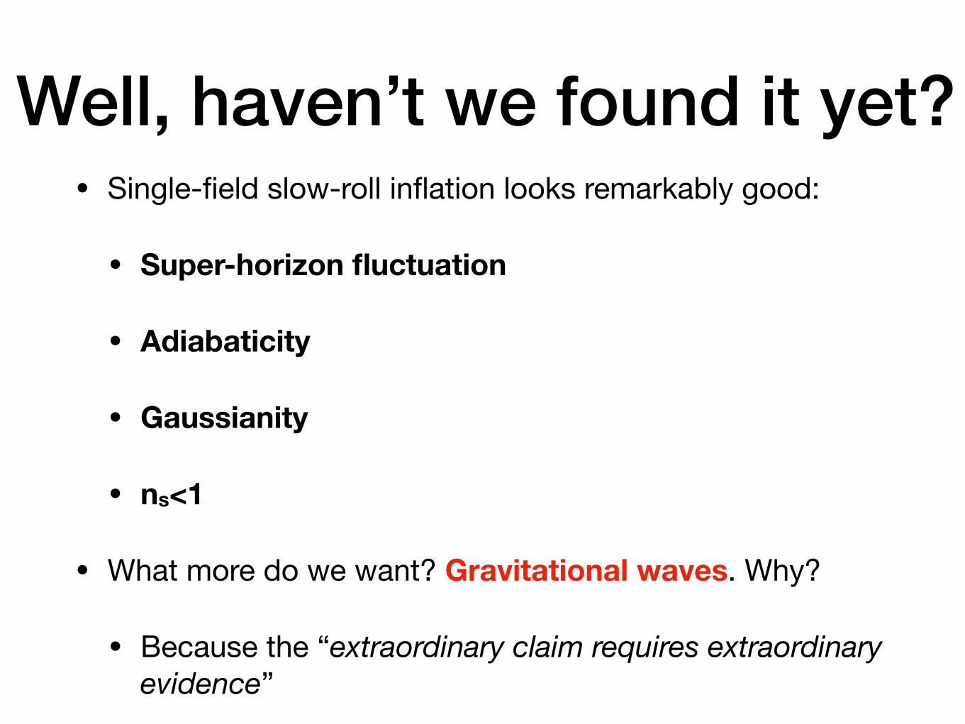
Well, haven’t we found it yet?• Single-field slow-roll inflation looks remarkably good:
• Super-horizon fluctuation
• Adiabaticity
• Gaussianity
• ns<1
• What more do we want? Gravitational waves. Why?
• Because the “extraordinary claim requires extraordinary evidence”
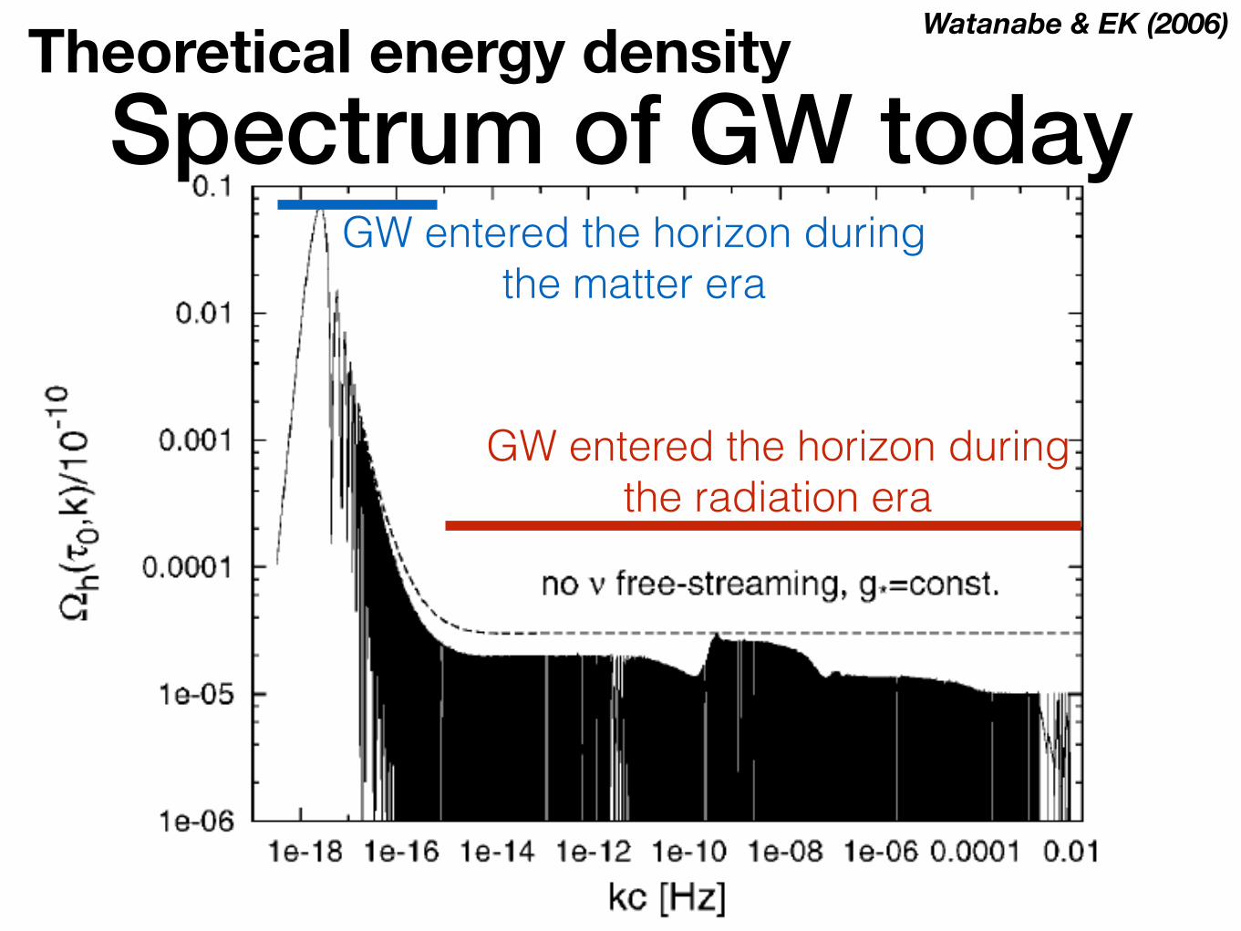
Theoretical energy density Watanabe & EK (2006)
GW entered the horizon during the radiation era
GW entered the horizon during the matter era
Spectrum of GW today
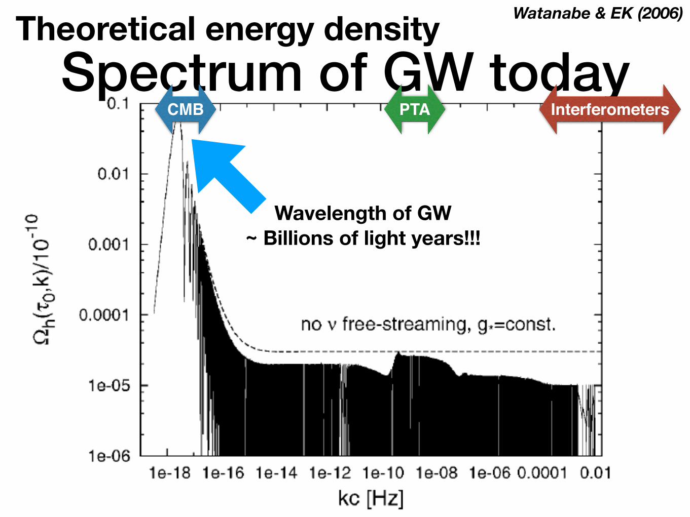
Spectrum of GW todayWatanabe & EK (2006)
CMB PTA Interferometers
Wavelength of GW ~ Billions of light years!!!
Theoretical energy density

You might not have noticed, but this conference has been very unique and remarkable

You might not have noticed, but this conference has been very unique and remarkable

You might not have noticed, but this conference has been very unique and remarkable
Gauge-fielders!Thanks for comments on the first part of my talk
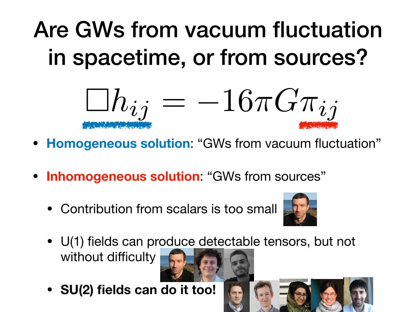
Are GWs from vacuum fluctuation in spacetime, or from sources?
• Homogeneous solution: “GWs from vacuum fluctuation”
• Inhomogeneous solution: “GWs from sources”
• Contribution from scalars is too small
• U(1) fields can produce detectable tensors, but not without difficulty
• SU(2) fields can do it too!
⇤hij = �16⇡G⇡ij
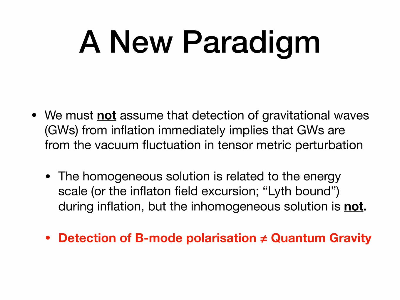
A New Paradigm
• We must not assume that detection of gravitational waves (GWs) from inflation immediately implies that GWs are from the vacuum fluctuation in tensor metric perturbation
• The homogeneous solution is related to the energy scale (or the inflaton field excursion; “Lyth bound”) during inflation, but the inhomogeneous solution is not.
• Detection of B-mode polarisation ≠ Quantum Gravity

From Matteo Fasiello
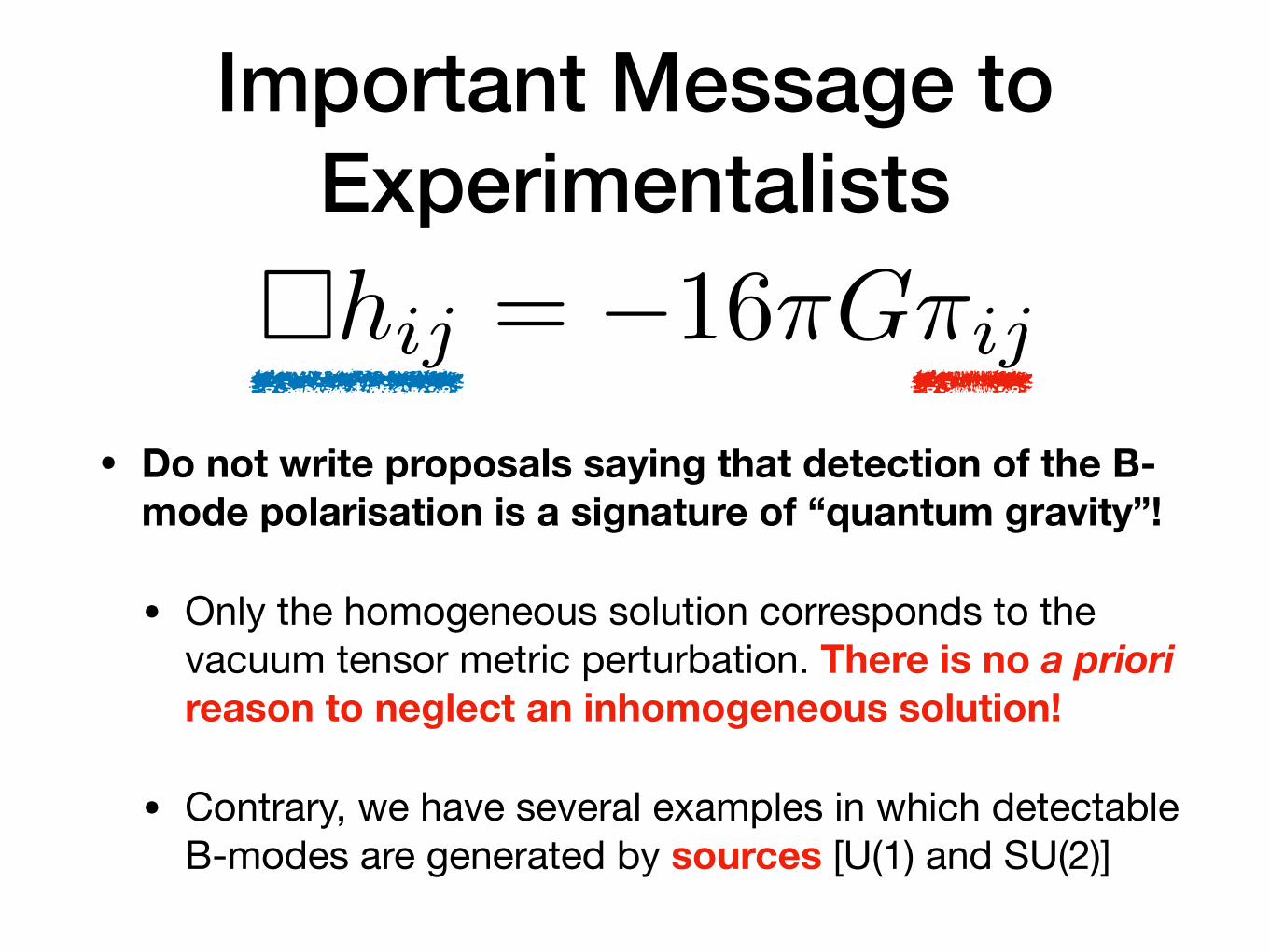
Important Message to Experimentalists
• Do not write proposals saying that detection of the B-mode polarisation is a signature of “quantum gravity”!
• Only the homogeneous solution corresponds to the vacuum tensor metric perturbation. There is no a priori reason to neglect an inhomogeneous solution!
• Contrary, we have several examples in which detectable B-modes are generated by sources [U(1) and SU(2)]
⇤hij = �16⇡G⇡ij

Experimental Strategy Commonly Assumed So Far1. Detect B-mode polarisation in multiple frequencies, to
make sure that it is the B-mode of the CMB
2. Check for scale invariance: Consistent with a scale invariant spectrum?
• Yes => Announce discovery of the vacuum fluctuation in spacetime
• No => WTF?

New Experimental Strategy: New Standard!
1. Detect B-mode polarisation in multiple frequencies, to make sure that it is the B-mode of the CMB
2. Consistent with a scale invariant spectrum?
3. Parity violating correlations (TB and EB) consistent with zero?
4. Consistent with Gaussianity?
• If, and ONLY IF Yes to all => Announce discovery of the vacuum fluctuation in spacetime
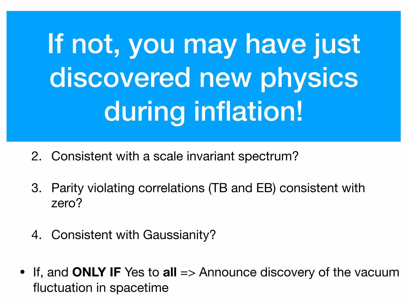
If not, you may have just discovered new physics
during inflation!

New Experimental Strategy: New Standard!
1. Detect B-mode polarisation in multiple frequencies, to make sure that it is the B-mode of the CMB
2. Consistent with a scale invariant spectrum?
3. Parity violating correlations (TB and EB) consistent with zero?
4. Consistent with Gaussianity?
• If, and ONLY IF Yes to all => Announce discovery of the vacuum fluctuation in spacetime
If not, you may have just discovered new physics
during inflation!
You would not have to worry about super-Planckian field excursion. Easier integration with fundamental physics?
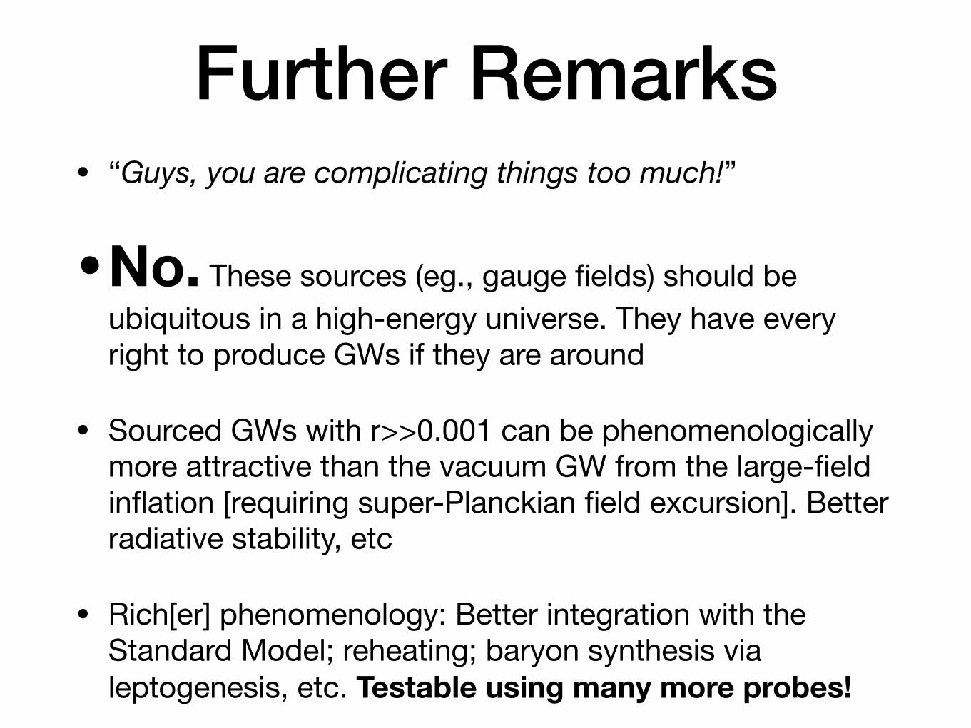
Further Remarks• “Guys, you are complicating things too much!”
•No. These sources (eg., gauge fields) should be ubiquitous in a high-energy universe. They have every right to produce GWs if they are around
• Sourced GWs with r>>0.001 can be phenomenologically more attractive than the vacuum GW from the large-field inflation [requiring super-Planckian field excursion]. Better radiative stability, etc
• Rich[er] phenomenology: Better integration with the Standard Model; reheating; baryon synthesis via leptogenesis, etc. Testable using many more probes!
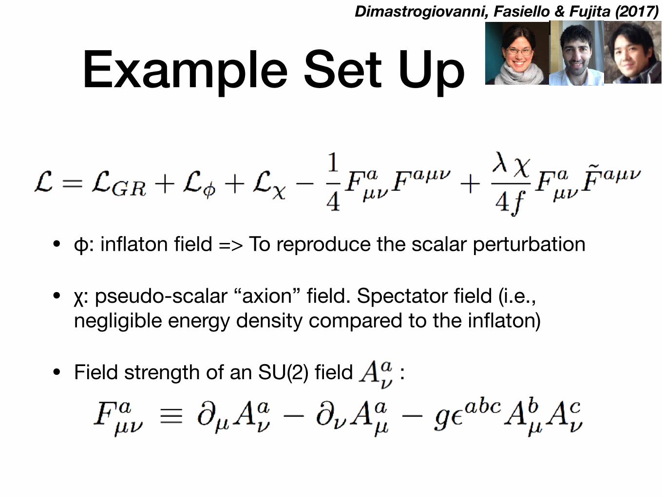
Example Set UpDimastrogiovanni, Fasiello & Fujita (2017)
• φ: inflaton field => To reproduce the scalar perturbation
• χ: pseudo-scalar “axion” field. Spectator field (i.e., negligible energy density compared to the inflaton)
• Field strength of an SU(2) field :
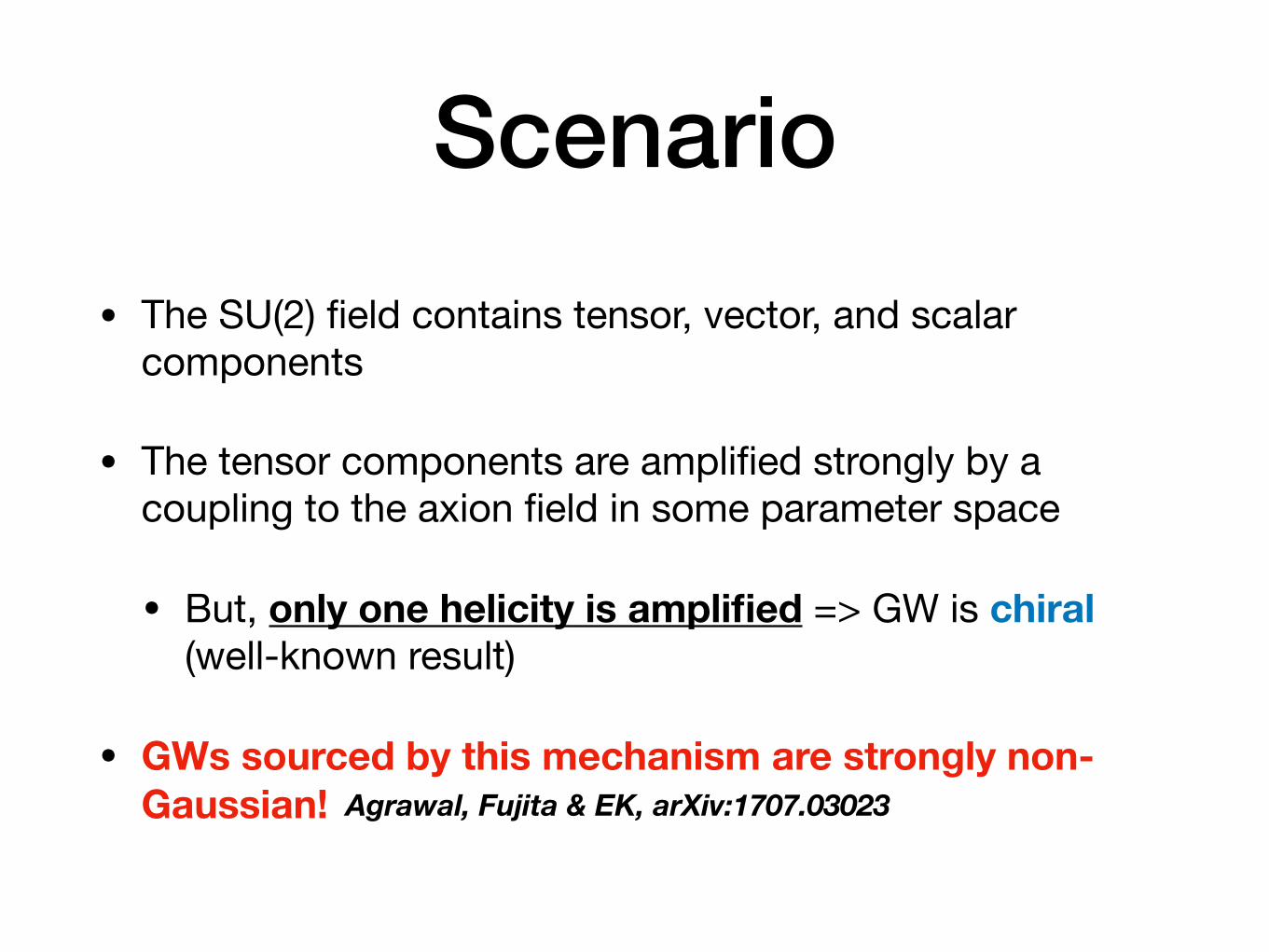
Scenario• The SU(2) field contains tensor, vector, and scalar
components
• The tensor components are amplified strongly by a coupling to the axion field in some parameter space
• But, only one helicity is amplified => GW is chiral (well-known result)
• GWs sourced by this mechanism are strongly non-Gaussian! Agrawal, Fujita & EK, arXiv:1707.03023
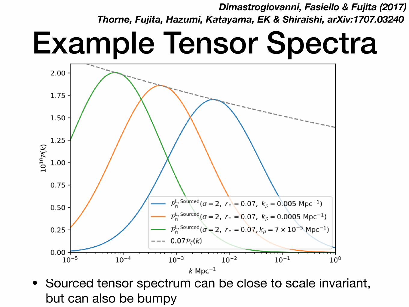
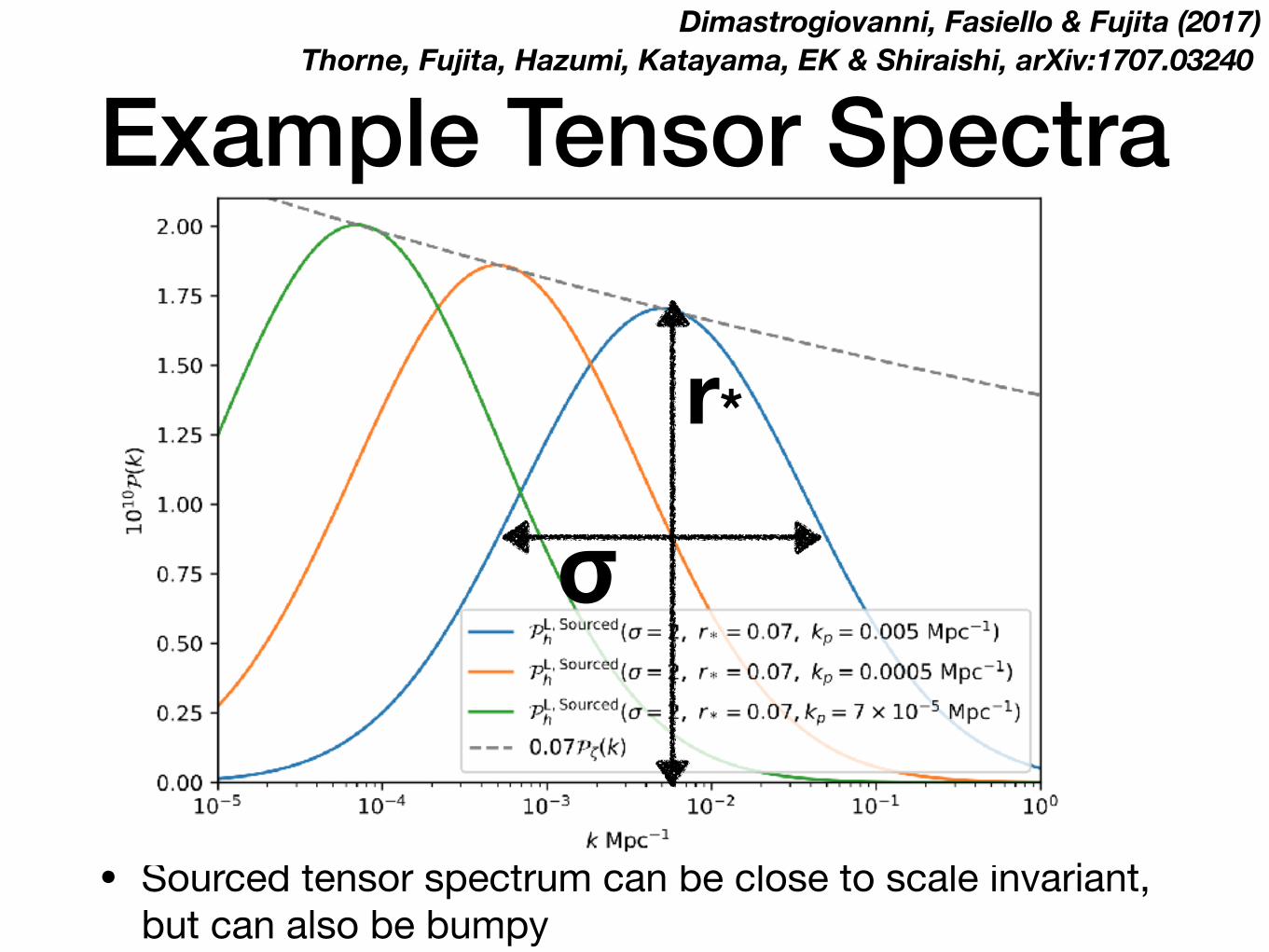
Example Tensor Spectra
• Sourced tensor spectrum can be close to scale invariant, but can also be bumpy
Thorne, Fujita, Hazumi, Katayama, EK & Shiraishi, arXiv:1707.03240Dimastrogiovanni, Fasiello & Fujita (2017)
Example Tensor Spectra
• Sourced tensor spectrum can be close to scale invariant, but can also be bumpy
Thorne, Fujita, Hazumi, Katayama, EK & Shiraishi, arXiv:1707.03240
σ
r*
Dimastrogiovanni, Fasiello & Fujita (2017)
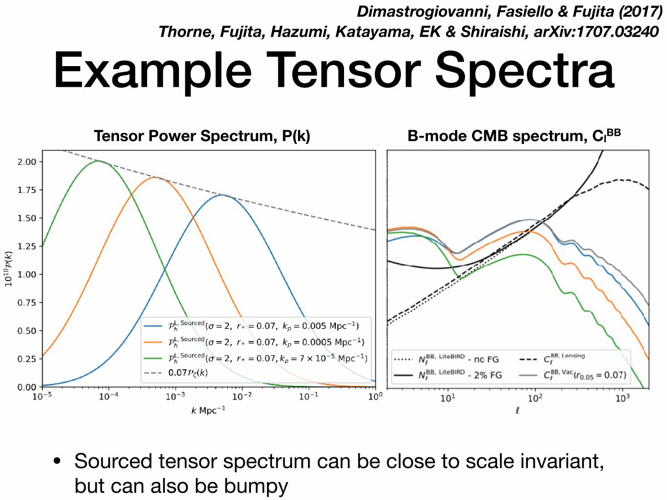
Example Tensor SpectraThorne, Fujita, Hazumi, Katayama, EK & Shiraishi, arXiv:1707.03240
Tensor Power Spectrum, P(k) B-mode CMB spectrum, ClBB
• Sourced tensor spectrum can be close to scale invariant, but can also be bumpy
Dimastrogiovanni, Fasiello & Fujita (2017)
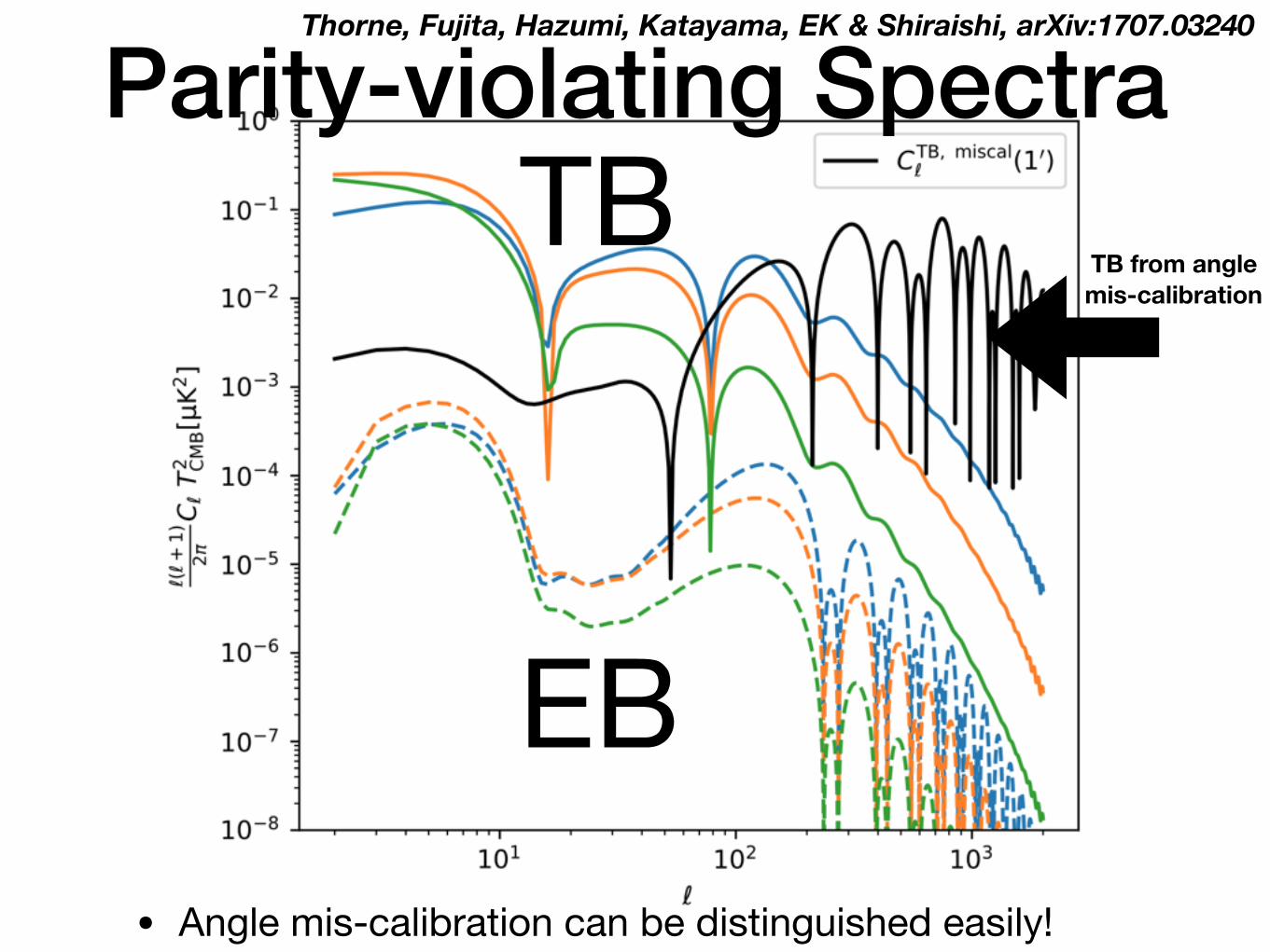
Parity-violating Spectra
• Angle mis-calibration can be distinguished easily!
Thorne, Fujita, Hazumi, Katayama, EK & Shiraishi, arXiv:1707.03240
EB
TBTB from angle mis-calibration
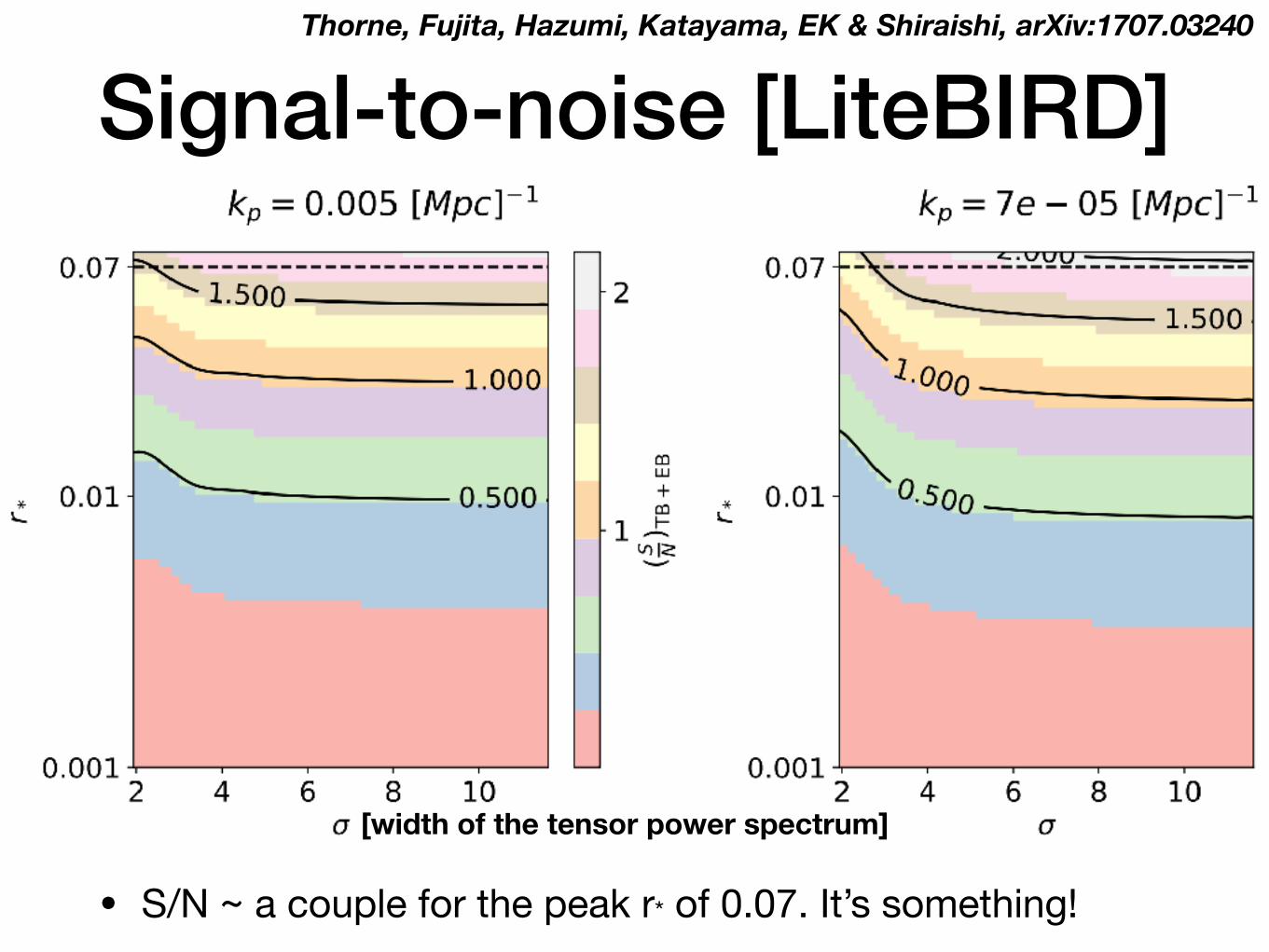
Signal-to-noise [LiteBIRD]
• S/N ~ a couple for the peak r* of 0.07. It’s something!
Thorne, Fujita, Hazumi, Katayama, EK & Shiraishi, arXiv:1707.03240
[width of the tensor power spectrum]
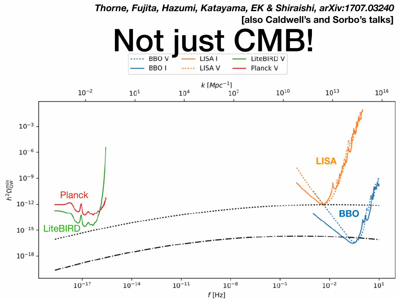
Thorne, Fujita, Hazumi, Katayama, EK & Shiraishi, arXiv:1707.03240[also Caldwell’s and Sorbo’s talks]
Not just CMB!
LISA
BBO
Planck
LiteBIRD
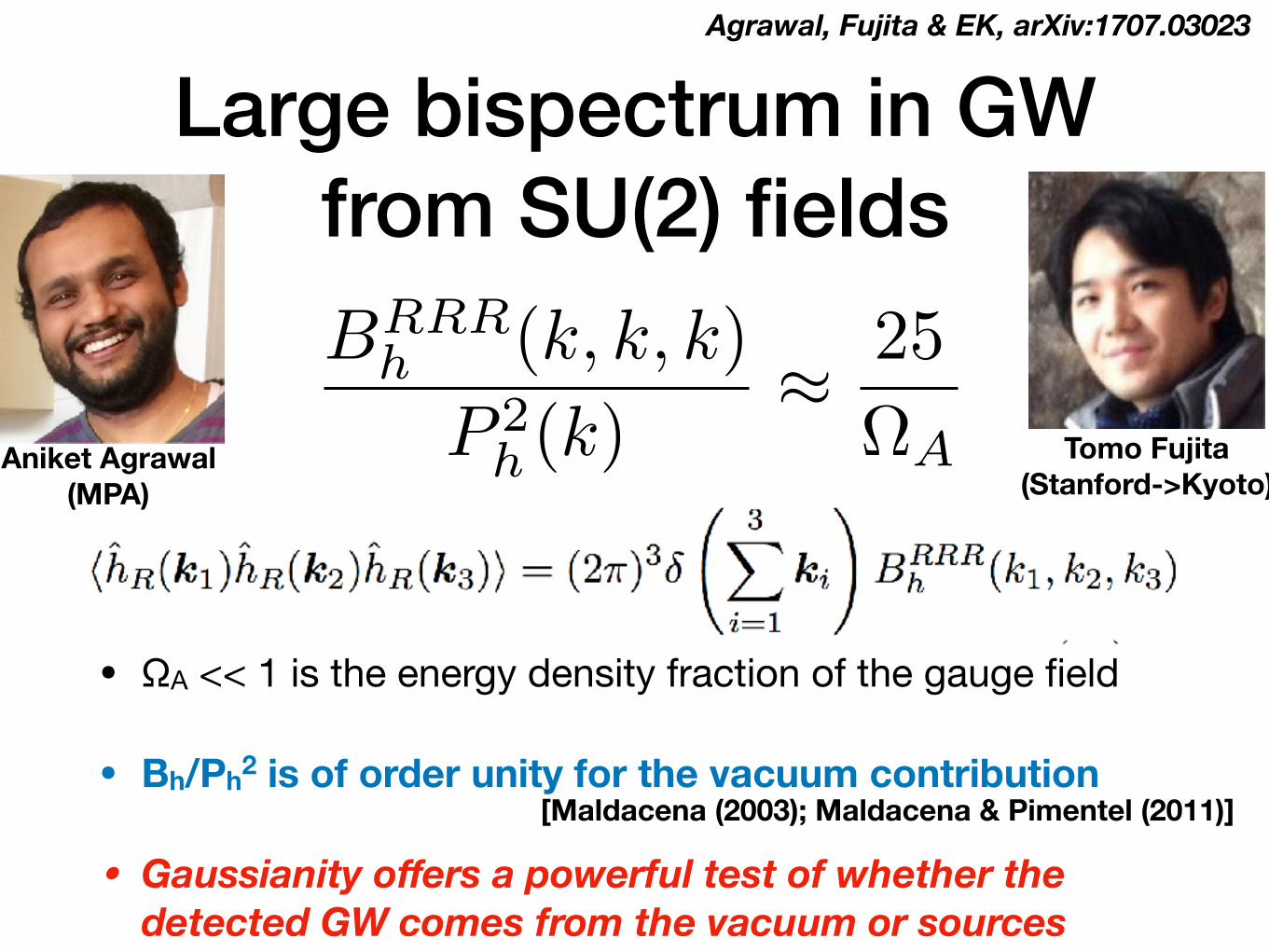
Large bispectrum in GW from SU(2) fields
• ΩA << 1 is the energy density fraction of the gauge field
• Bh/Ph2 is of order unity for the vacuum contribution
• Gaussianity offers a powerful test of whether the detected GW comes from the vacuum or sources
BRRRh (k, k, k)
P 2h (k)
⇡ 25
⌦AAniket Agrawal (MPA)
Tomo Fujita (Stanford->Kyoto)
Agrawal, Fujita & EK, arXiv:1707.03023
[Maldacena (2003); Maldacena & Pimentel (2011)]
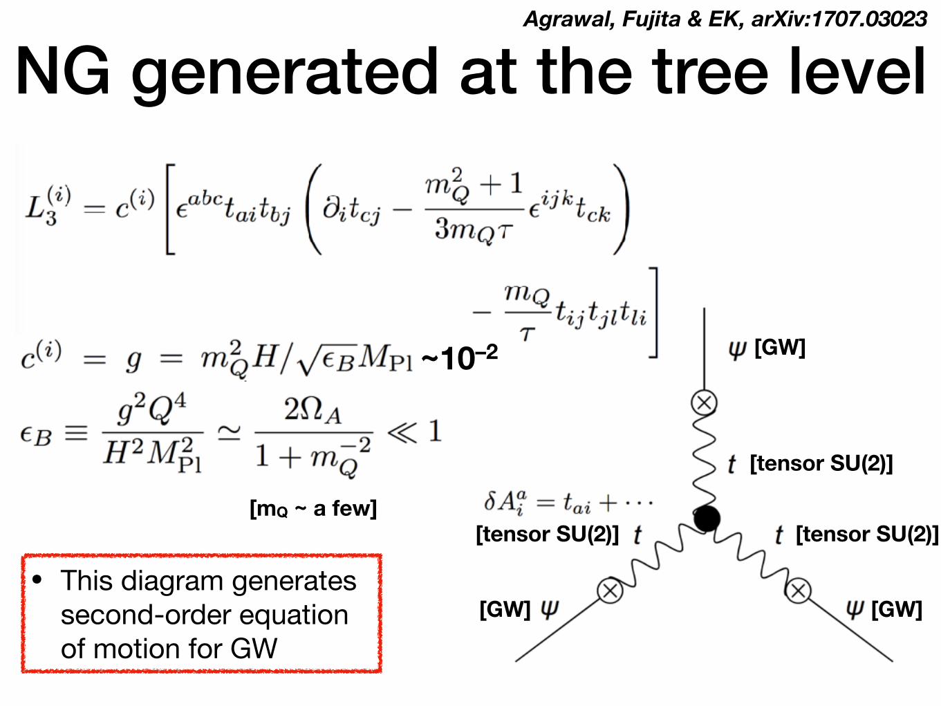
NG generated at the tree level
• This diagram generates second-order equation of motion for GW
[GW]
[GW][GW]
[tensor SU(2)]
[tensor SU(2)][tensor SU(2)][mQ ~ a few]
Agrawal, Fujita & EK, arXiv:1707.03023
~10–2

NG generated at the tree level
• This diagram generates second-order equation of motion for GW
[GW]
[GW][GW]
[tensor SU(2)]
[tensor SU(2)][tensor SU(2)][mQ ~ a few]
Agrawal, Fujita & EK, arXiv:1707.03023
BISPECTRUM+perm.
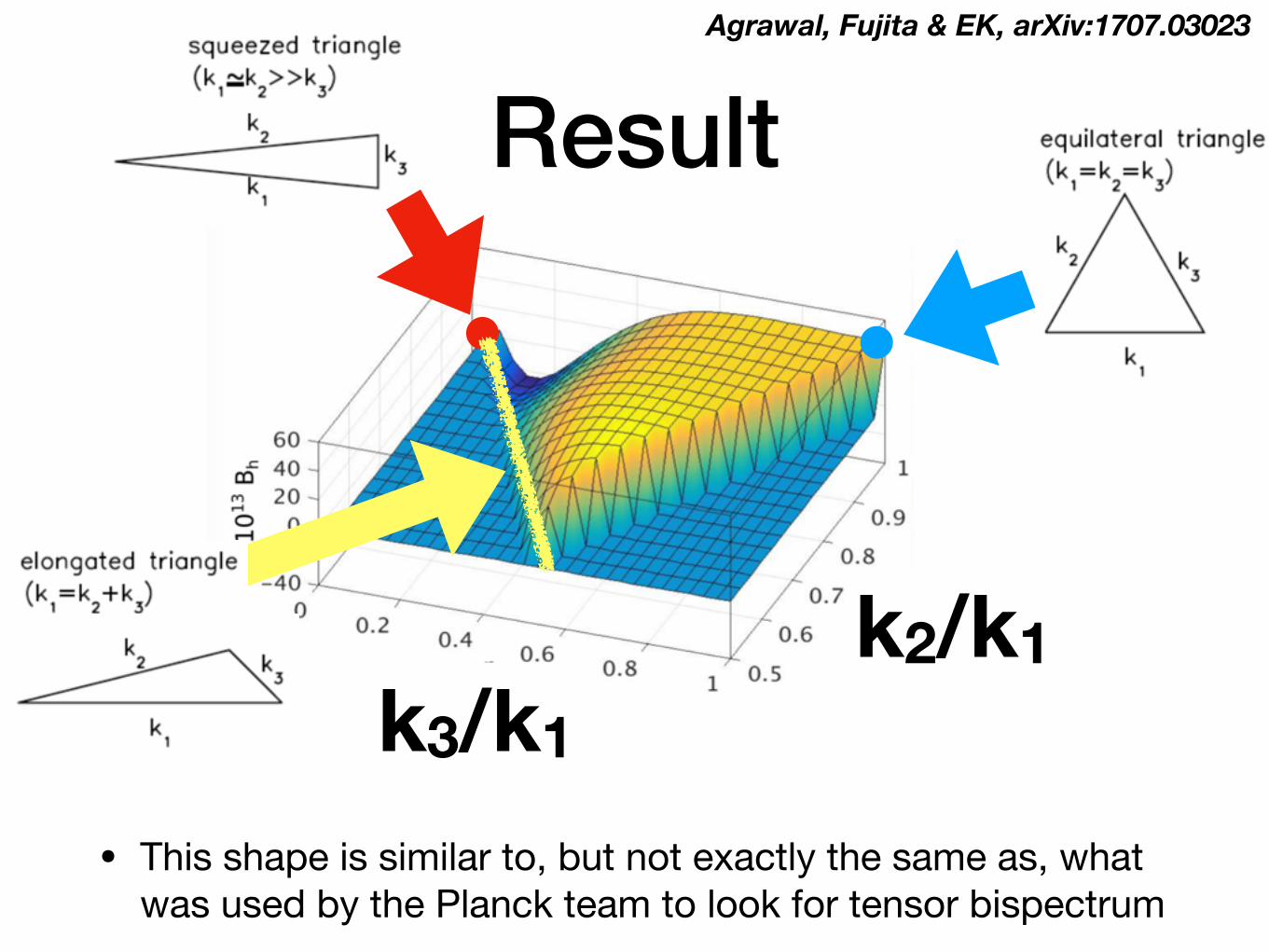
Result
• This shape is similar to, but not exactly the same as, what was used by the Planck team to look for tensor bispectrum
Agrawal, Fujita & EK, arXiv:1707.03023
k3/k1k2/k1
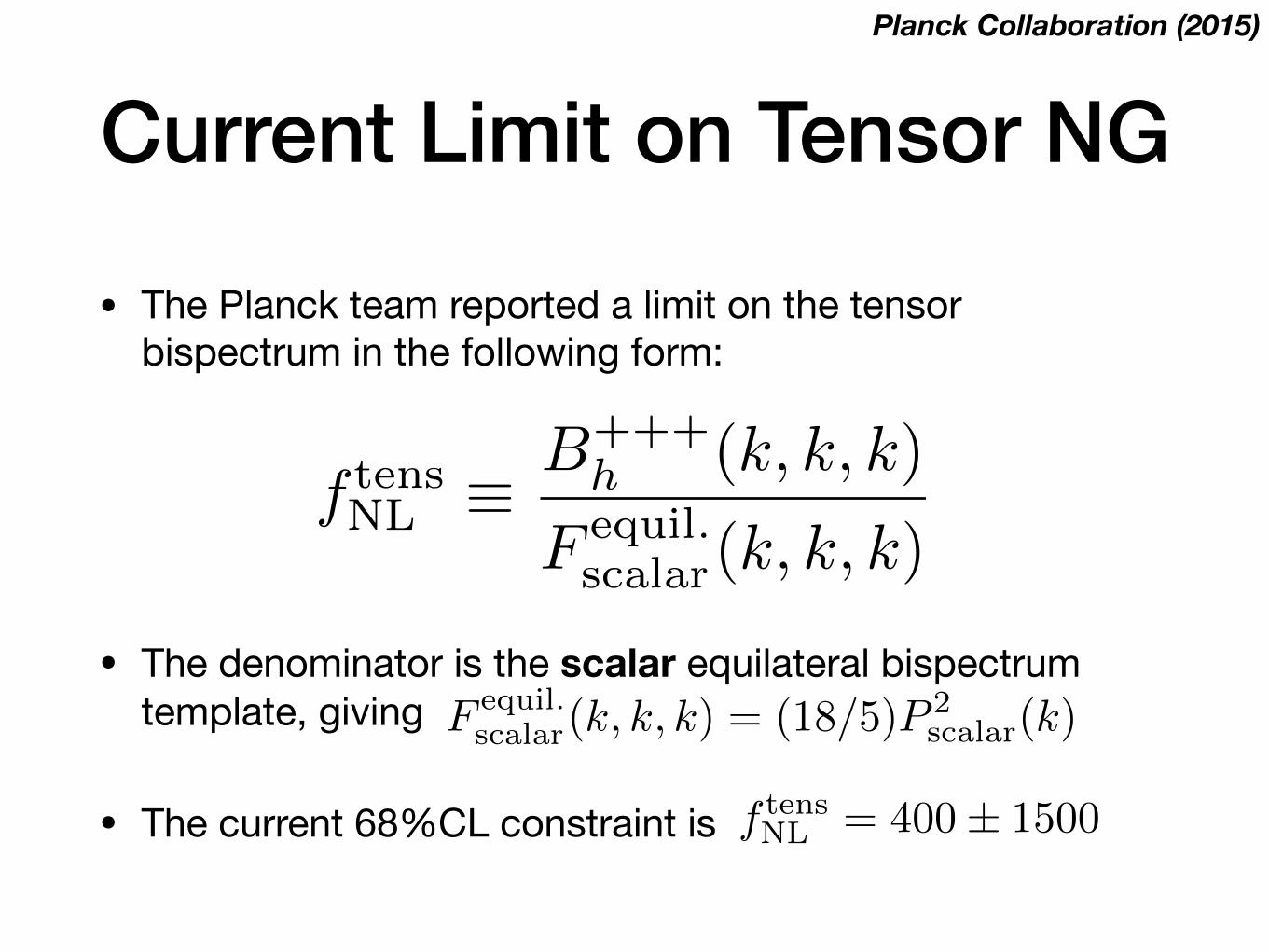
Current Limit on Tensor NG
• The Planck team reported a limit on the tensor bispectrum in the following form:
Planck Collaboration (2015)
f tensNL ⌘
B+++h (k, k, k)
F equil.scalar(k, k, k)
• The denominator is the scalar equilateral bispectrum template, giving F equil.
scalar(k, k, k) = (18/5)P 2scalar(k)
• The current 68%CL constraint is f tensNL = 400± 1500
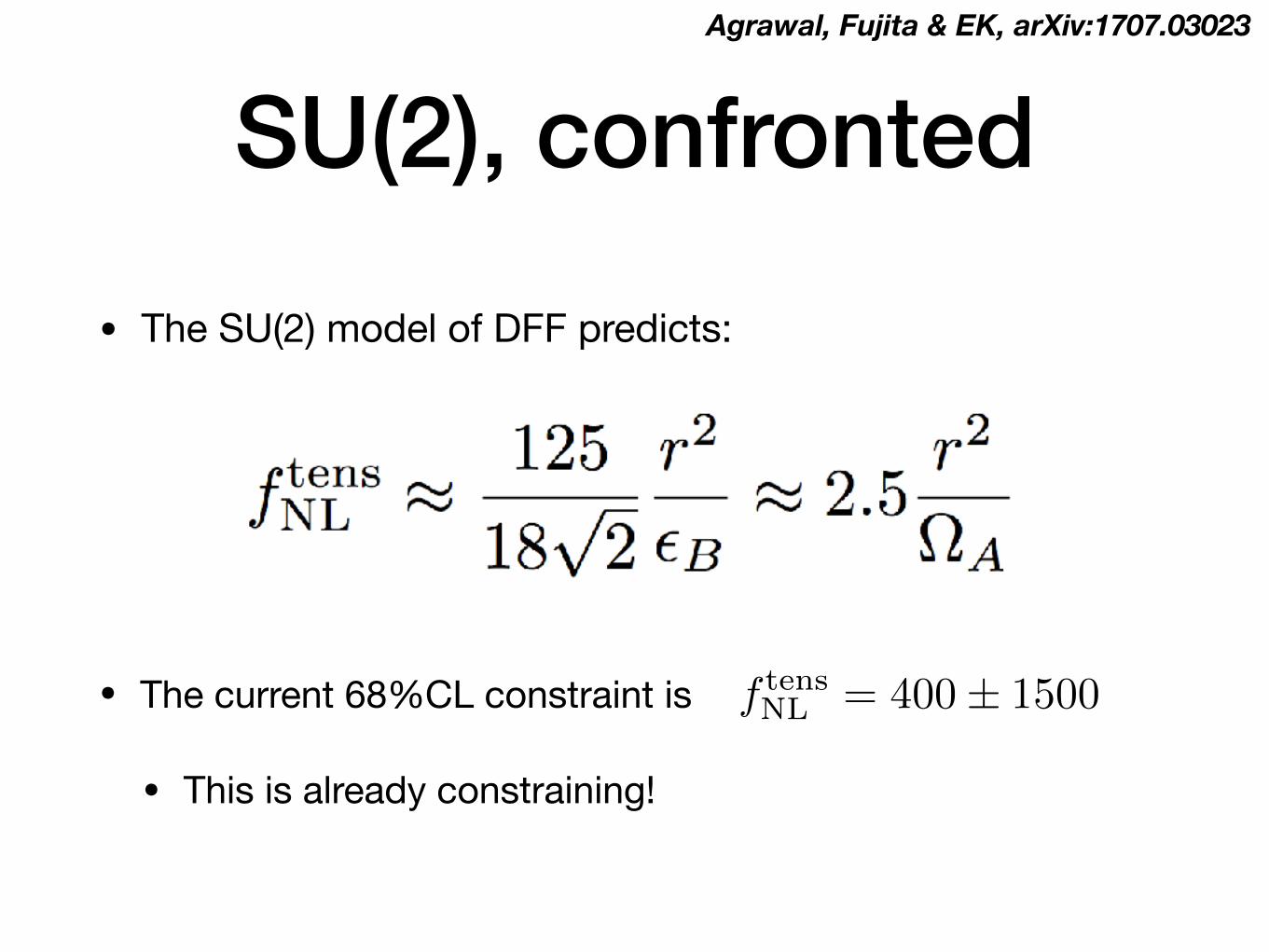
SU(2), confronted
• The SU(2) model of DFF predicts:
• The current 68%CL constraint is
• This is already constraining!
f tensNL = 400± 1500
Agrawal, Fujita & EK, arXiv:1707.03023
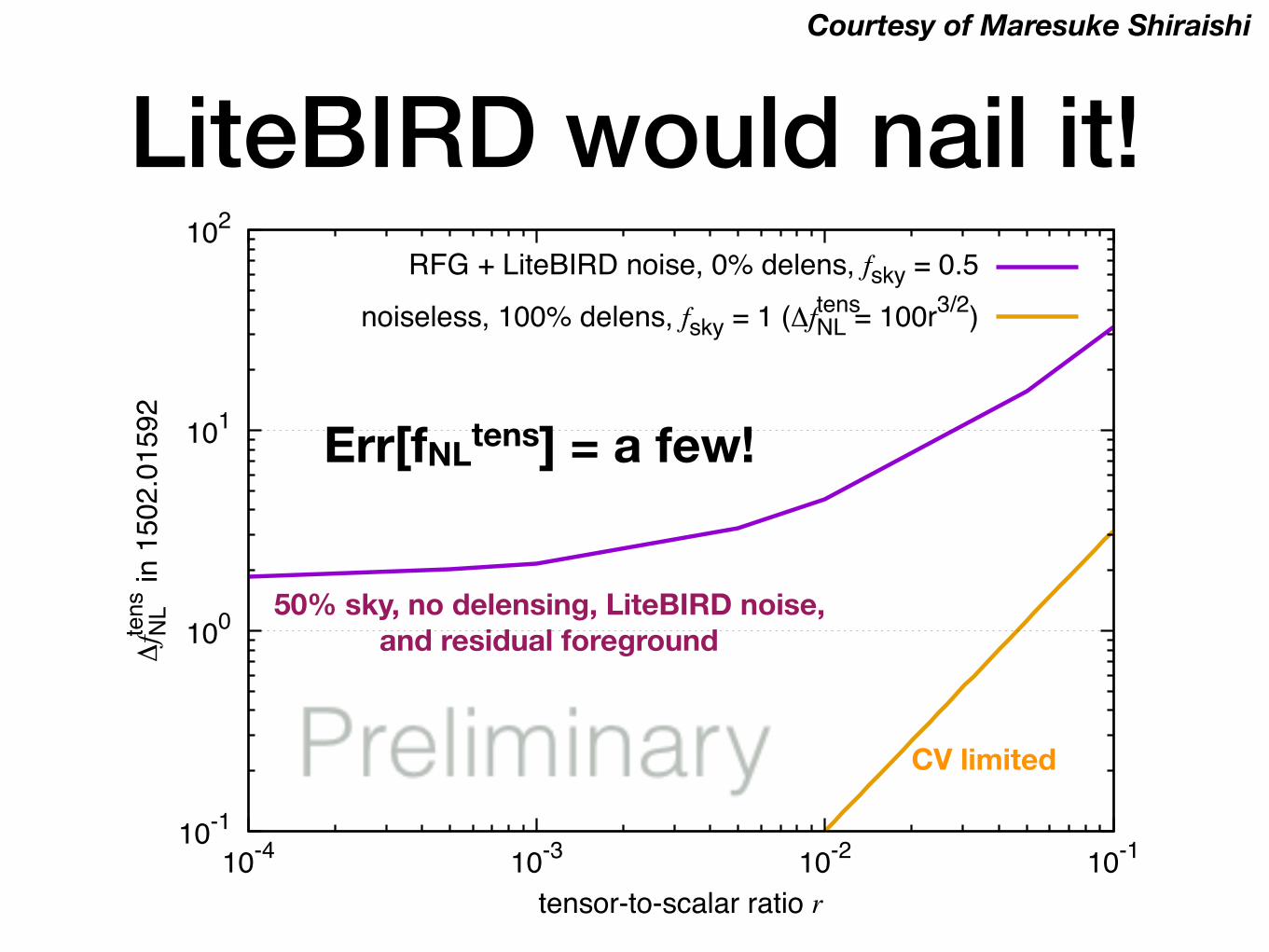
LiteBIRD would nail it!Courtesy of Maresuke Shiraishi
∆fte
nsN
L i
n 15
02.0
1592
tensor-to-scalar ratio r
RFG + LiteBIRD noise, 0% delens, fsky = 0.5
noiseless, 100% delens, fsky = 1 (∆ftensNL = 100r3/2)
10-1
100
101
102
10-4 10-3 10-2 10-1
50% sky, no delensing, LiteBIRD noise, and residual foreground
CV limited
Err[fNLtens] = a few!
What is LiteBIRD?
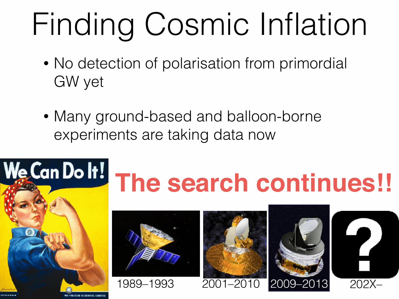
• No detection of polarisation from primordial GW yet
• Many ground-based and balloon-borne experiments are taking data now
The search continues!!
Finding Cosmic Inflation
1989–1993 2001–2010 2009–2013 202X–
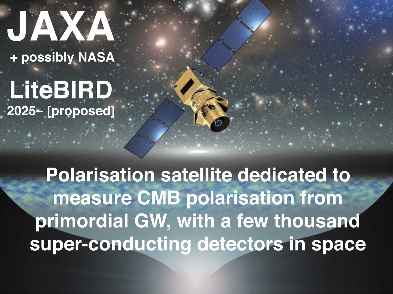
ESA2025– [proposed]
JAXA+ possibly NASA
LiteBIRD2025– [proposed]
Polarisation satellite dedicated to measure CMB polarisation from
primordial GW, with a few thousand super-conducting detectors in space

ESA2025– [proposed]
JAXA+ possibly NASA
LiteBIRD2025– [proposed]
Target sensitivity: σ(r=0) = 0.001
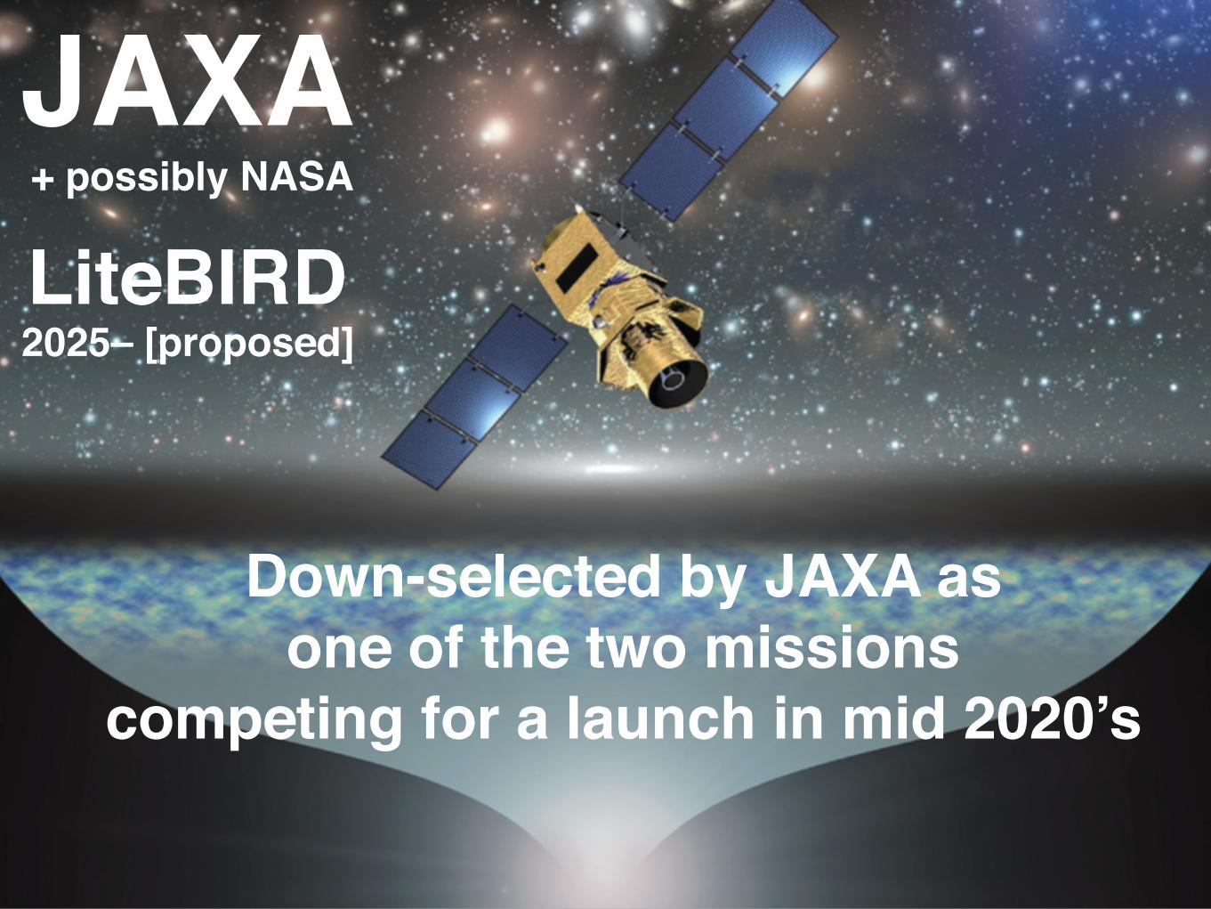
ESA2025– [proposed]
JAXA+ possibly NASA
LiteBIRD2025– [proposed]
Down-selected by JAXA as one of the two missions
competing for a launch in mid 2020’s
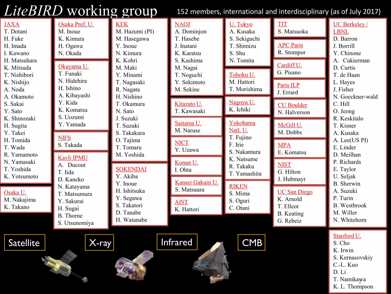
LiteBIRD working group 152 members, international and interdisciplinary (as of July 2017)JAXAT. DotaniH. FukeH. ImadaI. KawanoH. MatsuharaK. MitsudaT. NishiboriK. NishijoA. Noda A. OkamotoS. Sakai Y. SatoK. ShinozakiH. SugitaY. TakeiH. TomidaT. WadaR. YamamotoN. YamasakiT. YoshidaK. Yotsumoto
Osaka U.M. NakajimaK. Takano
Osaka Pref. U.M. InoueK. KimuraH. OgawaN. Okada
Okayama U.T. FunakiN. HidehiraH. IshinoA. KibayashiY. KidaK. KomatsuS. UozumiY. Yamada
NIFSS. Takada
Kavli IPMUA. DucoutT. IidaD. KanekoN. KatayamaT. MatsumuraY. SakuraiH. SugaiB. ThorneS. Utsunomiya
KEKM. Hazumi (PI) M. HasegawaY. InoueN. Kimura K. KohriM. MakiY. MinamiT. NagasakiR. NagataH. NishinoT. OkamuraN. Sato J. SuzukiT. SuzukiS. TakakuraO. Tajima T. TomaruM. Yoshida
Konan U.I. Ohta
NAOJA. DominjonT. HasebeJ. InataniK. KaratsuS. KashimaM. NagaiT. NoguchiY. SekimotoM. Sekine
Saitama U.M. Naruse
NICTY. Uzawa
SOKENDAIY. AkibaY. InoueH. IshitsukaY. SegawaS. TakatoriD. TanabeH. Watanabe
TITS. Matsuoka
Tohoku U.M. HattoriT. Morishima
Nagoya U.K. Ichiki
Yokohama Natl. U.T. FujinoF. IrieS. NakamuraK. NatsumeR. TakakuT. Yamashita
RIKENS. MimaS. OguriC. Otani
APC ParisR. Stompor
CU BoulderN. Halverson
McGill U.M. Dobbs
MPAE. Komatsu
NISTG. HiltonJ. Hubmayr
Stanford U.S. ChoK. IrwinS. KernasovskiyC.-L. KuoD. LiT. NamikawaK. L. Thompson
UC Berkeley / LBNLD. BarronJ. BorrillY. ChinoneA. CukiermanD. CurtisT. de HaanL. HayesJ. FisherN. Goeckner-waldC. HillO. JeongR. KeskitaloT. KisnerA. KusakaA. Lee(US PI)E. LinderD. MeilhanP. RichardsE. TaylorU. SeljakB. SherwinA. SuzukiP. TurinB. WestbrookM. WillerN. Whitehorn
UC San DiegoK. ArnoldT. ElleotB. KeatingG. Rebeiz
CMBInfraredSatellite X-ray
Kansei Gakuin U.S. Matsuura
Paris ILPJ. Errard
Cardiff U.G. Pisano
2
Kitazato U.T. Kawasaki
U. TokyoA. KusakaS. SekiguchiT. ShimizuS. ShuN. Tomita
AISTK. Hattori
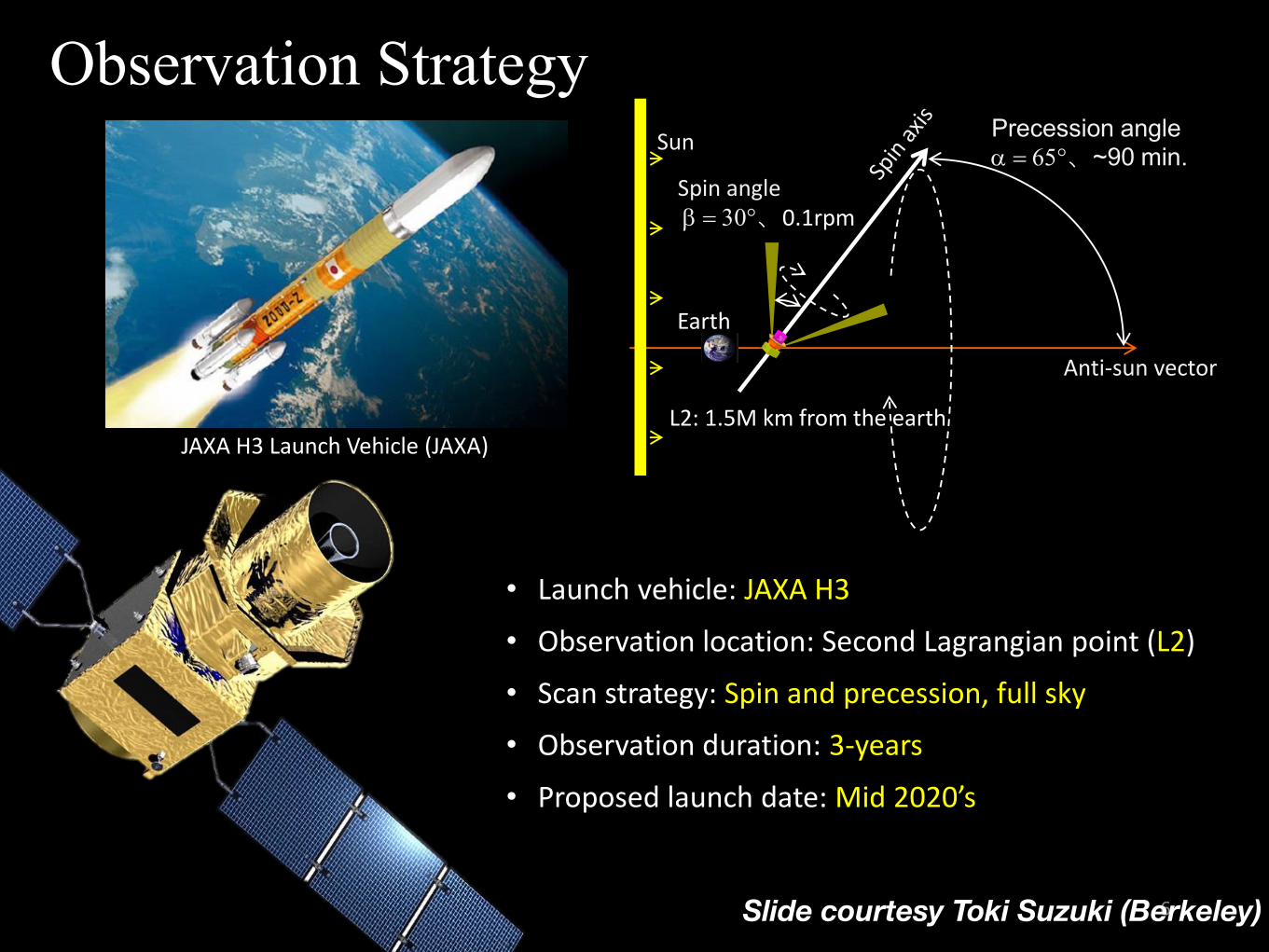
Observation Strategy
6
• Launch vehicle: JAXA H3
• Observation location: Second Lagrangian point (L2)
• Scan strategy: Spin and precession, full sky
• Observation duration: 3-years
• Proposed launch date: Mid 2020’s
JAXA H3 Launch Vehicle (JAXA)
Anti-sun vector
Spin angle
b = 30°、0.1rpm
SunPrecession anglea = 65°、~90 min.
L2: 1.5M km from the earth
Earth
Slide courtesy Toki Suzuki (Berkeley)
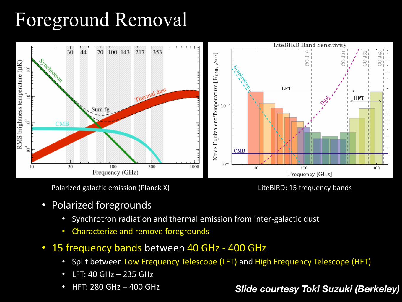
• Polarized foregrounds• Synchrotron radiation and thermal emission from inter-galactic dust
• Characterize and remove foregrounds
• 15 frequency bands between 40 GHz - 400 GHz• Split between Low Frequency Telescope (LFT) and High Frequency Telescope (HFT)
• LFT: 40 GHz – 235 GHz
• HFT: 280 GHz – 400 GHz
Foreground Removal
7
Polarized galactic emission (Planck X) LiteBIRD: 15 frequency bands
Slide courtesy Toki Suzuki (Berkeley)

Instrument Overview
8
LFTHFT
LFT primary mirror
LFTSecondarymirror
HFT
HFT FPUSub-K Cooler
HFT Focal Plane
LFT Focal Plane
Readout
• Two telescopes• Crossed-Dragone (LFT) & on-axis refractor (HFT)
• Cryogenic rotating achromatic half-wave plate• Modulates polarization signal
• Stirling & Joule Thomson coolers• Provide cooling power above 2 Kelvin
• Sub-Kelvin Instrument• Detectors, readout electronics, and a sub-kelvin cooler
400 mm
Sub-Kelvin Instrument
Cold Mission System
Stirling & Joule Thomson Coolers
Half-wave plate
Mission BUS System
Solar Panel
200 mm ~ 400 mm
Slide courtesy Toki Suzuki (Berkeley)
Summary
• Single-field slow-roll inflation looks very good in everything we have looked at in the scalar perturbation
• Super-horizon, isotropic, adiabatic, Gaussian, and ns<1
• But we want more to find definitive evidence for inflation: primordial gravitational waves with the wavelength of billions of light years
⇤hij = �16⇡G⇡ij
Summary• This conference has seen a new direction
in the B-mode search: GWs from sources!
• Experimental designs should pay attention to:
• Non scale-invariance,
• Parity-violating correlations, and
• Non-Gaussianity
• LiteBIRD in an excellent position to not only find GWs but also to characterise them

Many thanks to the organisers!
After the fabulous banquet on the ship on July 19