Find a Job Now, Start Working LaterDoes Unemployment Insurance Subsidize Leisure?

(Job market paper)

Marjolaine Gauthier-LoisellePrinceton University

September 2011

Abstract

Distorting incentives is a major concern when implementing Unemployment In-surance (UI). In particular, UI benefits tend to decrease job search and increasethe reservation wage. Yet, UI could also be prone to moral hazard through anotherunexplored channel: postponing job start upon finding a job. This paper developsa theoretical job search model that allows for a delayed job start. Then, the extentto which unemployed individuals delay job start after finding a job is assessed usingthe Canadian Survey of Labour and Income Dynamics. I find that 17% of all bene-fits paid are paid to individuals who have already found a job, but have not startedworking yet. I find that individuals who accepted an offer before benefit exhaustiondelay job start by 3.9 weeks on average, whereas the average delay is respectively 1.8and 2.3 weeks for those who accepted a job after exhaustion and for non-recipients.The survival analysis shows that the job starting rate upon acceptance of a job offeris much higher both in the month prior to exhaustion and after the benefits areexhausted, as well as for non-recipients. Although no causal effect can be formallyidentified, this suggests that some individuals take advantage of the availability ofUnemployment Insurance benefits to postpone job start.

*I would like to thank my advisor, Henry Farber, Andreas Mueller, as well as par-ticipants to the Graduate Labor Workshop and the Public Finance Working Group atPrinceton University for helpful questions and comments. Research was conducted atMcGill’s Quebec Inter-University Center for Social Statistics and Statistics Canada andI would like to thank Statistics Canada analysts for their great work. I also acknowledgefinancial support from the Social Sciences and Humanities Research Council of Canadaand from the Fonds Qubcois de la recherche sur la socit et la culture.

1 Introduction

Unemployment Insurance (UI) serves the goal of providing a safety net in case of a job

loss.1 However, UI benefits create an opportunity for unemployed workers to put less

effort into looking for a job and going back to work. As many researchers have found,

more generous benefits tend to increase unemployment duration (Card and Levine, 2000;

Van Ours and Vodopivec, 2006; Lalive, Van Ours and Zweimueller, 2006; Lalive, 2008).

In traditional job search models, unemployed individuals receiving UI benefits search less

intensively and have higher reservation wages, leading to longer unemployment spells (e.g.

Mortensen,1977).2 Yet, unemployed individuals could also take advantage of UI benefits

through another unexplored channel: postponing job start after accepting a job offer.

Upon finding a job, an unemployed individual receiving UI benefits might be deciding to

take a few extra weeks off work without the stress of finding a job. Although intuitive,

this idea was proposed only recently (Boone and Van Ours, 2009) and little is known

about the magnitude of the tendency to postpone job start and its potential cost for the

society. The goal of this paper is to investigate the importance of the delay between job

offer and job start, as well as its determinants.

The moral hazard induced by Unemployment Insurance has not only been documented

through longer unemployment durations, but also through a spike in the unemployment

exit rate at benefit exhaustion (Moffit, 1985; Katz and Meyer, 1990; Meyer, 1990).3 Post-

poning job start after accepting an offer could explain, at least partly, these empirical

findings. In fact, when raising the idea that unemployed individuals could strategically

delay job start, Boone and Van Ours (2009) do not study the delay per se, rather, they

want to explain the spike in the job starting rate at benefit exhaustion. Indeed, they

find supporting evidence of their theoretical model, which implies that delaying job start

could cause the spike. However, their data set doesn’t allow them to observe the delay

between job offer and job start, nor do most major data sets. The lack of information on

1 In the literature, the usual term for this type of program is Unemployment Insurance. However, in1996, the program was renamed Employment Insurance in Canada. To avoid confusion, I will stick tothe traditional name of the program.

2 Chetty (2008) differs in attributing this increase in unemployment duration to liquidity constraintsrather than distortion in search behaviour.

3 Card, Chetty and Weber (2007) point out that the spike is much smaller for the job starting ratethan for the unemployment exit rate.

1

job offer date is probably the main reason why the delay between job offer and job start

still remains undocumented.

This paper investigates the importance of the tendency to delay, both in terms of

frequency and length, as well as its determinants. I first develop a theoretical job search

model that allows for a delay between job offer and job start. Then, I investigate the

delay behaviour and its determinants using the Canadian Survey of Labour and Income

Dynamics. The contribution of this paper is twofold. First, acknowledging the existence

of the delay, there is a need for search models that incorporate this feature. This paper

contributes to the job search literature by developing a non-stationary job search model

that allows for a delay between job offer and job start. Second, it extends the literature

on the effects of Unemployment Insurance on unemployment spells by documenting a new

channel of moral hazard using a unique data set that provides information on job offer

and job start dates along with detailed socio-demographics and administrative tax record

information.

Traditional job search models assume that a job starts as soon as it is accepted, leaving

no room for a delay between job offer and job start. The model presented here builds on

the work of Van den Berg (1990), where employers make take-it-or-leave-it job offers to

unemployed workers. Both his model and my model allow for non-stationarity, although

Van den Berg (1990) model allows for non-stationarity in a more general setting, whereas

I allow non-stationarity in UI benefits only. The core difference is that a job offer entails

both a wage and a start date in my model, whereas an offer consists only of a wage in

Van den Berg (1990). It is important to note that the model developed by Boone and

Van Ours (2009) does allow for delay between job offer and job start, but since it aims

at explaining the spike in the job starting rate at benefit exhaustion, it doesn’t model

acceptance nor rejection of job offers by the worker and, therefore, is not a job search

model per se.

The model implies that there should not be a spike in the job acceptance rate at

benefit exhaustion, but rather the rate should remain high and stable. Empirically, I find

that the job acceptance rate is higher both in the month prior to exhaustion and after ex-

haustion. Even though the point estimate is larger in the month prior to exhaustion, it is

2

not significantly different from the coefficient after exhaustion, so there is no spike per se.

However, I find a spike in the job starting rate prior to exhaustion as expected from pre-

vious studies. The model predicts that jobs with longer delays should be associated with

higher wages for individuals accepting an offer after exhaustion and for non-recipients,

which is confirmed by the data. More generally, the model presented here implies that

unemployed individuals adjust their acceptance or rejection of job offers according to the

start date and their eligibility to UI benefits, leading to a new, unexplored, form of moral

hazard.

In the empirical analysis, I decompose the unemployment spell into two parts: the

duration of unemployment until a job offer is accepted and the delay between job offer

and job start. Although the latter has been left out of the existing literature, I find that

unemployed workers delay job start substantially after accepting a job offer. Individuals

who accepted an offer before benefit exhaustion postpone job start by 3.9 weeks on av-

erage, and 54% delay job start by more than two weeks. In comparison, individuals who

accepted an offer after exhaustion delay job start by 1.8 weeks on average and only 35%

of individuals delay job start by more than two weeks. Similarly, individuals who did

not receive UI benefits delay job start by 2.3 weeks on average and 40% delay do so for

more than two weeks. Acknowledging that non-recipients and individuals who accepted

an offer after benefit exhaustion differ from those who accepted an offer before benefit

exhaustion, and thus don’t constitute reliable control groups, the differences in the delay

behaviour remain striking and suggest that the delay has a strategic component, i.e. the

delay is reflective of individuals’ preferences. Overall, 17% percent of all Unemployment

Insurance benefits paid is paid to individuals who have already found a job, but have not

started working yet. Furthermore, even if we allow for a two-week institutional waiting

period before job start, the cost of the delay above the institutional threshold remains as

high as 11% of all benefits paid.

The survival analysis shows that the job starting rate upon job acceptance is much

higher after benefit exhaustion and for non-recipients. This finding provides further evi-

dence that the delay is not solely institutional, but has a strategic component. I also find

that individuals accepting an offer early in their spell are much less likely to resume work

quickly. Personal characteristics such as age, gender and education don’t seem to affect

3

delay behaviour by much. However, having children is correlated with a longer delay

for single parent families in some specifications. Re-employment job characteristics also

seem to matter. Jobs in the public sector are less likely to start quickly after job offer,

and unionized jobs are more likely to start quickly in some specifications. To summarize,

the empirical analysis suggests that some individuals take advantage of the availability of

benefits to postpone job start.

The paper is set-up as follows. Section 2 introduces the theoretical model. Section

3 presents the data and descriptive statistics. Section 4 presents the empirical analysis.

Finally, section 5 concludes.

2 A Job Search Model with Delay

The model developed here extends the non-stationary search model presented by Van den

Berg (1990) to incorporate delay between job offer and job start. The model considers

the acceptance behavior of an unemployed individual eligible to receive UI benefits for

a period of time T at the beginning of his unemployment spell, where job offers consist

of a wage, w, and a start date after a waiting period, τ , and arrive at random intervals

following a homogeneous Poisson process with arrival rate λ.

The model has two important features: non-stationarity and multi-dimensionality

of job offers. First, as in Van den Berg (1990), the non-stationarity implies that the

optimal acceptance rule varies over the course of the unemployment spell. Here, the non-

stationarity is introduced by the finite duration of UI benefits, whereas the Van den Berg

(1990) model encompasses a broader class of non-stationarity. Secondly, in the model

presented here, a job offer consists of a wage and a waiting period until the job starts,

τ . Other models also include multi-dimensional job offers. For example, Blau (1991),

Bloemen (2008) and Shephard (2009) considered job offers with wages and hours. I fol-

low Blau (1991) by considering the utility flow associated with all dimensions of the job

offer.4 In that case, the optimal acceptance rule maximizes the expected present value of

the utility of accepting a job net of search cost. This rule is known to have the “reser-

4The alternative is to consider the monetary value of the non-wage characteristics.

4

vation utility property”, i.e. an offer is accepted if and only if the utility flow associated

with the offer is above a certain threshold that may vary accordingly with the dimensions

of the offer. Note that since the model is non-stationary, the reservation utility will vary

over the unemployment spell.5

The setting of the model is as follow (a list of the symbols is available in the appendix).

There is an infinite search horizon and job offers arrive at random intervals following a

non-homogeneous Poisson process with a constant, exogenous and known arrival rate, λ.

Workers then accept or reject the offer, but there is no recall of offers previously declined

and workers are not allowed to continue searching after accepting a job offer (this also

precludes on-the-job search). Once a job has started, it lasts forever at a constant wage.

A job offer consists of a wage, w ∈ [0,W ], and a waiting period until the job starts,

τ ∈ [0,M ]. Job offers are random drawings from a wage and wait time distribution with

the distribution function F (w, τ), the conditional distribution F1(w|τ) and the partial dis-

tribution F2(τ) known and constant over time. For convenience, unemployment duration

and calendar time match, i.e. unemployment starts at t = 0.

The wage is allowed to depend on the delay between job offer and job start, but the

process generating such a relationship is not in the scope of this paper. In particular, both

a positive and a negative relationship could be rationalized. For example, there could be

a negative relationship if firms which know in advance that they will need a new worker at

given date post early offers with a long delay at low wage hoping to get a deal, gradually

increasing the offered wage as the starting date approaches. Alternatively, there could be

a positive relationship if firms which are looking for specific human capital start searching

earlier to ensure a good match and offer a higher wage to compensate for the waiting

period. Another possibility is that early knowledge of a vacancy depends on other firms’

characteristics that are related to wages. In this partial equilibrium search model, I am

agnostic about the process generating the relationship between wages and delay, but I

allow for such a relationship.

5For a more complete review of job search models, see Rogerson, Shimer and Wright (2005) for a

theory oriented survey and Van den Berg (1999) and Eckstein and Van den Berg (2007) a for survey of

empirical estimations of job search models.

5

Individuals at time t derive utility from leisure, l(t), and consumption, c(t), and there

are no savings or borrowing. When employed, workers consume their wage, w, and enjoy

leisure, l(t) = le. If unemployed, they consume B(t), the sum of their home-production

and benefits if any, and enjoy leisure, l(t) = lu > le. Unemployed individuals are eligible

to receive UI benefits for a period T from the beginning of a new unemployment spell,

thus B(t) = B if t < T . B(t) = b < B if t ≥ T . Note that T and B(t) can vary

from one individual to another, but the subscript indicating the individual is omitted

for simplification. The worker chooses his acceptance strategy such that the implied

consumption and leisure schedule maximizes the expected value of his lifetime utility,

U(c, l). Thus, the worker maximizes:

E(U(c, l)) = E

∫ ∞t

e−ρ(s−t)u(c(s), l(s))ds (1)

subject to

(c(s), l(s)) =

(w, le) if working,

(B(s), lu) if not working.

where 0 < ρ <∞ is the worker’s subjective discount rate and u(c(s), l(s)) is the utility

flow with uc > 0, ul > 0, ucc < 0 and ull < 0.

Diamond (1971) showed that if workers are homogeneous and there is no on-the-job

search, then there is no wage dispersion: all firms post the common reservation wage.

To generate wage dispersion, I will follow Albrecht and Axell (1984) and Eckstein and

Wolpin (1990) and assume that workers differ in their opportunity cost of employment,

and thus have different reservation wages for a given start date. In particular, B(t) and

T are allowed to vary from one individual to another. When workers have different reser-

vation wages, firms will attract different types of workers depending on the wage they

offer. In particular, firms offering a low wage will attract workers with a low reservation

wage, whereas firms offering a high wage will attract both low and high reservation wage

workers. This leads to a non-degenerate wage distribution in equilibrium, when firms are

indifferent between offering low and high wages.

6

2.1 Worker’s problem

In this setting, the unemployed worker has to choose whether to accept or reject the job

offer whenever he receives one. Following the job search literature, the optimal strategy

for the individual is to accept the job that maximizes the expected present value of life-

time utility net of search costs. Even though there is no direct cost of search, there is

an indirect cost in the form of foregone earnings. A job will be accepted if the expected

present value of the lifetime utility of accepting the offer, V e(w, τ, t), is larger than or

equal to the expected present value of lifetime utility of rejecting the offer, V u(t).

The expected present value of lifetime utility of accepting in period t a job that starts

in a period of time τ at wage w is

V e(w, τ, t) =

∫ t+τ

t

e−ρ(v−t)u(B(v), lu)dv +e−ρτ

ρu(w, le). (2)

The first term of the equation above represents the value while delaying job start after

accepting a job offer, whereas the second term represents the value once the individual

starts to work.

The job offer arrival process implies that the probability that the next offer arrives

at time s ≥ t conditional on being unemployed at time t has a distribution function

G(s; t) = 1− e−λ(s−t). The expected present value of lifetime utility of being unemployed

in period t can then be written as

V u(t) =

∫ ∞t

[

∫ s

t

e−ρ(v−t)u(B(v), lu)dv + e−ρ(s−t)Ew,τ ;s(max(V e(w, τ, s), V u(s))]dG(s; t).

(3)

This equation is the expectation over the next job offer’s arrival time of the sum of the

value of being unemployed until the next job offer arrives and the value of the optimal

choice between accepting or rejecting the next offer.

Let u(τ, t) be the reservation utility, defined as the utility flow such that the unem-

ployed worker is indifferent (in period t) between remaining unemployed or starting to

work in τ periods and receiving a utility flow u(τ, t) once the job has started. The solu-

tion to the worker’s problem is such that any offer (w, τ) with u(w, le) ≥ u(τ, t) will be

accepted in period t. Let Q(u|τ) = Pr(u(w, le) ≤ u|τ) be the distribution of the utility

7

flow once the job has started conditional on the delay between job offer and job start.

Note that Q(u|τ) = F1(w∗|τ), where u = u(w∗, le).

Proposition 1. Reservation utility

a. Case t ≥ T :

After benefit exhaustion, the worker’s problem becomes stationary. The reservation

utility is then constant in t, so u(τ, t) = u(τ) and satisfies

u(τ) = u(b, lu) +λ

ρ

∫ M

0

∫ u(W,le)

u(z)

e−ρ(z−τ)(1−Q(u|z))dudF2(z). (4)

Moreover, (i) u(τ, t) is increasing in τ .

b. Case t < T :

Before exhaustion, u(τ, t) satisfies

∂u(τ, t)

∂t= ρu(τ, t)− ρu(B(t+ τ), lu)− λ

∫ M

0

∫ u(W,le)

u(z,t)

e−ρ(z−τ)(1−Q(u|z))dudF2(z).

(5)

Furthermore, (i) u(τ, t) is decreasing and concave in t for t < T ,

(ii) u(τ, t) is decreasing in τ for τ ∈ [0, T − t) if u(B, lu) > u(w, le) for the lowest

accepted wage given a start date (increasing otherwise),

(iii) u(τ, t) is increasing in τ for τ ∈ [T − t,∞).

Proof. See the appendix.

Proposition 1a implies that when the benefits are exhausted, a job offer is accepted if

the utility flow once the job has started is at least as high as the utility flow when unem-

ployed plus the discounted expected increase in the utility flow from accepting another

offer in the future. Proposition 1a (i) comes from the idea that when the benefits are

exhausted, the worker prefers to start working sooner than later for any acceptable offer.

If it were not the case, the worker would prefer to remain unemployed forever than to

work under those conditions and the offer would be rejected. Therefore, to accept a job

with a delayed start date, the worker would need to be compensated for the lost income

during the delay period by a higher utility flow (i.e. higher wage) once the job has started.

The reservation utility increasing with the delay implies that, after exhaustion, an offer

is more likely to be accepted if the delay is shorter, other things being equal. Moreover,

8

since the marginal value of consumption is positive (uc > 0), the lowest acceptable wage

for a job increases with the delay until job start. Thus, offers with a long delay will be

accepted only if they entail a higher wage. Consequently, a positive relationship between

wages and delay should appear in the data whenever the individual does not receive UI

benefits after accepting a job offer.

Proposition 1b (i) and uc > 0 imply that, as the exhaustion date approaches, the un-

employed individual is willing to accept a lower wage for a given delay. Consequently, the

minimum acceptable wage for a given delay decreases over the jobless spell until exhaus-

tion, then remains constant. In particular, the model predicts that the job acceptance

rate is increasing until exhaustion, then remains high and stable. More precisely, the job

acceptance rate in t conditional on not having accepted a job before, θo(t), is simply the

probability of receiving a job offer that is accepted, that is the probability that the wage

and start date offered give a utility flow larger than the reservation utility once the job

starts (Pr(u(w, le) ≥ u(τ, t))). Therefore,

θo(t) = λ

∫ M

z=0

(1−Q(u(z, t)|z))dF2(z). (6)

We can see easily that the job acceptance rate increases whenever the reservation utility

decreases, and vice-versa. Thus, the rate at which job offers are accepted is increasing

until exhaustion, then constant. Consequently, there is no spike in the job acceptance rate

at benefit exhaustion, but rather an increased rate that remains stable after exhaustion.6

Proposition 1b (ii) states the worker would rather delay job start and collect UI ben-

efits than to start working now if the period utility of being unemployed with UI benefits

is large enough. More precisely, the worker is willing to forego future earnings in order to

remain unemployed. As a result, a negative relationship between wage and delay should

emerge from the data. Yet, if u(B, lu) ≤ u(τ, t), the intuition becomes similar to that

of proposition 1a: the worker would prefer to start working sooner than later and would

need a higher wage to accept an offer with longer delay. Since only some individuals

6A richer model including search intensity could generate a spike in the job acceptance rate if leisure

and consumption were substitutes. Then, instead of remaining at a high level following benefit exhaustion,

the job acceptance rate would decrease due to a reduced search effort (increased leisure) to compensate

the reduced consumption.

9

with high value of staying at home with benefits would like to delay, the direction of the

relationship between wage and delay is ambiguous. Finally, proposition 1b (iii) implies

that in the case where the job offer is before exhaustion, but with a delay long enough

that worker resume work after exhaustion (τ ≥ T − t), the worker would rather start to

work sooner than later once the benefits are exhausted and he would want a higher wage

to accept an offer with a slightly longer delay. Yet, the overall effect of delaying could be

either positive or negative. Proposition 1b (iii) only compares job offers with a start date

after exhaustion to those with a further start date. It remains ambiguous whether start-

ing a job a little after exhaustion would be better than starting as soon as the job is offered.

Furthermore, propositions 1b (ii) and (iii) imply that for a given wage and offer time,

the probability that a job is accepted is maximized when the job start date coincides with

exhaustion if the benefits are large enough. Consequently, there are more offers starting

at exhaustion which are accepted and the job starting rate spikes at exhaustion. Simi-

larly, propositions 1b (ii) and (iii) imply that individuals who receive a job offer before

exhaustion are more likely to accept an offer with a longer delay between job offer and

job start.

To summarize, the lowest acceptable utility flow varies according to the delay between

job offer and job start and the UI benefits remaining at the time of job offer. The reserva-

tion utility reaches its minimum with respect to time after exhaustion, whereas it reaches

its minimum with respect to delay when the job start date coincides with exhaustion if

the benefits are large enough. Since job offers affect the utility flow only through changes

in wage, we have that the lowest acceptable wage is higher for a long delay if the job

offer is received after exhaustion, whereas the relationship between wages and delay is

ambiguous if the job is offered before exhaustion.

The empirical implications of the model are summarized in the following proposition

and are tested in the empirical analysis (section 4).

Proposition 2. Under the appropriate assumptions on the distribution of (w, τ) and if

UI benefits are large enough, the model has the following empirical implications:

a. Jobs that start at benefit exhaustion are more likely to be accepted, creating a spike

in the job starting rate at benefit exhaustion.

10

b. There is no spike in the job acceptance rate at benefit exhaustion, rather the job

acceptance rate increases until exhaustion, then remains constant.

c. Longer delays are more likely to be accepted by individuals who receive an offer before

benefit exhaustion.

d. Wages are positively correlated with delay between job offer and job start if the

offer is received after benefit exhaustion, whereas the direction of the correlation is

ambiguous if the offer is received before exhaustion.

The model presented in this section assumes that individuals change their acceptance

decision of a job offer depending on the timing of job start. Therefore, although the delay

between job offer and job start is dictated by the employers, workers take advantage of

UI benefits to accept jobs that start later. So, individuals strategically delay job start in

the sense that the delay is reflective of preferences. The following sections assess whether

this idea of strategic delay is supported empirically.

3 Data and Descriptive Statistics

3.1 Data

To study the delay between job offer and job start, we need a data set that has information

about both the job offer and job start date. This information is provided in the Cana-

dian Survey of Labour and Income Dynamics (SLID), as well as detailed survey data on

demographic characteristics and financial information from administrative tax records.7

The SLID is an annual household survey conducted by Statistics Canada, which follows

households for 6 years. A new panel starts every three years and consists of roughly

30,000 individuals.8 The data used in this paper cover the period from 1993 to 2006.9

Additionally, to account for sampling design and non-random attrition, all results are

7Respondents need to give permission to be linked with administrative tax records. Over 80% of the

observations were linked with tax records in my sample. A fourth of the remaining observations had

income information collected from the SLID survey and the others had income information completely

imputed by Statistics Canada.8More information on the SLID can be found at http://www.statcan.gc.ca.9All financial variables are adjusted for inflation using the Consumer Price Index (available from

CANSIM) based on 2002 (CPI2002 = 100).

11

derived using the combined panel weights provided by Statistics Canada.

The sample of jobless spells of adults in the workforce is constructed as follows. The

sample is restricted to individuals from 20 to 65 years old who are neither retired nor

full-time students with at least one jobless spell starting during the survey period. In-

dividuals with a health condition preventing work are excluded from the sample. The

sample also precludes individuals who have been recalled from a previous employer as

their job search behavior is different (Krueger and Mueller, 2010). For the same reason,

individuals not looking for a job at the beginning of their spell because they expect to be

recalled are also excluded.10 To avoid the influence of outliers, spells with delay between

job offer and job start above the 99th percentile are discarded from the sample, so that

the longest delay in the sample lasts 30 weeks. Both UI recipients and non-recipients are

included in the analysis, although it is understood the differences in behaviour can’t be

identified as a causal effect of UI benefits, since the eligibility status and the decision to

apply for benefits are endogenous.

Individuals who quit the labor force at some point during their spell are not necessar-

ily excluded from the sample. The reason is that individuals who found a job but have

not started to work yet are considered unemployed only if the job is to start within the

next four weeks. If the waiting period is longer than four weeks, these individuals are

classified as out of the labor force. Since we are precisely interested in this waiting period,

we have to include individuals with a delay longer than four weeks. However, individuals

out of the labor force for more than a year are excluded from the sample. Consequently,

when I refer to unemployment spells or unemployed individuals in this paper, I do not

refer to the traditional definition that excludes jobless individuals not actively seeking

work. Rather, I respectively refer to unemployment spells and unemployed individuals

as temporary jobless spells and jobless individuals attached to the labor market. Since

the sample includes some individuals not actively seeking work, the observed spells could

be longer on average than it would if the sample were only constituted of unemployed

10These exclusions imply that the sample does not include individuals who did not look for work

because they expected and are indeed recalled, but also individuals who looked for another job but end

up being re-employed by the same employers, as well as individuals not looking for work at the beginning

of their spell because they expect to be recalled but who are finally re-employed by a different employer.

12

individuals defined in the traditional sense.

Data on both the jobless spells and the re-employment jobs are needed in order to

perform the analysis of the delay between job offer and job start. However, the structure

of the data is such that one can extract the data for job spell history or for jobless spell

history, but the data does not readily include the sequence of jobs and jobless spells.

Thus, I first extracted the data for jobless periods at the individual level, then matched

them with data from previous and following employment using start and end dates of job

and jobless spells, as well as monthly main job identifiers when one of the afore mentioned

dates were unavailable. Similarly, I extracted the SLID data for monthly receipts of UI

benefits and matched it with the employment history. Unfortunately, the data do not in-

clude the number of weeks eligible or exhaustion date. Therefore, I imputed the number

of weeks of benefits according to the rules specified under the Unemployment Insurance

program(described in the following section). Then, the number of weeks eligible is used

to compute the exhaustion date, taking into account the two weeks waiting period before

the start of benefits if applicable.

One major concern with survey data is measurement error due to recall. Recalling the

date of a job offer might be especially prone to measurement error. In particular, there is

a distinct bunching on the 1st, 2nd, 15th, 16th, 30th,and 31st day of the month. Moreover,

32% of individuals report that the job was offered the very same day as it started, and

23% report being offered the job on either Saturday or Sunday, both of which seem much

to high to be the true proportion. One way to deal with the measurement error is to

allow for unobserved heterogeneity in the survival analysis. Moreover, if UI recipients

are more likely to incorrectly report an offer date that is closer to the start date because

they are afraid of penalties, then my estimates would be biased downward. Nonetheless,

in spite of the measurement errors, I do find results indicating that delay has a strategic

component and that its magnitude is considerably large. These findings suggest that the

delay between job start and job offer deserves researchers’ attention and should be studied

with more reliable data in the future.

13

3.2 Unemployment Insurance in Canada

Since 1996, the Canadian UI program is called the “Employment Insurance”. After serving

a two-week waiting period, unemployed workers can receive benefits for a period ranging

from 19 to 50 weeks. The length of benefits varies with the unemployment rate in the

economic region and the number of hours worked. For example, an individual who was

working full-time in the year prior to the spell in a region with an unemployment rate

between 7% and 8% is eligible to 45 weeks of benefits.11

The base replacement rate is 55% of the insurable earnings, up to a maximum benefit

of $413/week.12 The insurable earnings are defined as the average weekly earnings over

the last 26 weeks. However, for those who have not work all weeks, the weekly insured

earnings is calculated by dividing the total earnings in the last 26 weeks by either the

number of weeks worked or the “divisor” number, whichever is the largest. The “divisor”

is a number ranging from 22 to 14 that decreases with the unemployment rate. For

families with income below $25,921, the replacement rate is supplemented up to 80%.

Eligibility to this program depends on the number of hours worked in the previous 52-

week period or the period since the last unemployment spell (whichever is the shortest).

Depending on the unemployment rate at the time of filing the claim, the minimum number

of insurable hours of work ranges from 420 to 700. For those in the work force for the first

time and those re-entering the work force after an absence of 2 years need 910 hours to

qualify. Moreover, those who quit without just cause, are fired for misconduct, refuse or

are unavailable to accept suitable employment are ineligible for benefits. For more details

on the UI program, see http://www.hrsdc.gc.ca/eng/employment/ei/.

11Between 420 and 1400 hours worked, an increase of 70 hours worked increases the benefits eligibility

by one week, whereas between 1400 and 1820 hours worked, 35 additional hours increase the benefits

entitlement by one week. Also, for an unemployment rate from 6% to 15%, an increase of one percentage

point of the unemployment rate expands benefit eligibility by two weeks.12In 2007, the maximum benefit was increased for the first time since 1996.

14

3.3 Descriptive Statistics

Previous literature looked at the unemployment duration as a whole. For comparability

purpose, I will reproduce this analysis before decomposing the total jobless spell duration

into the time until a job offer is accepted and the subsequent delay until job start. Figure

1 shows the distribution of the completed duration of jobless spells. UI recipients have

longer spell duration than non-recipients, with the median spell lasting 4 months and

the modal spell lasting 3 months, whereas the median spell length for non-recipients is

one month and the modal spell length is less than a month. This is partly due to non-

recipients accepting job offer earlier in their spell than UI recipients as shown in figure

2. In particular, those who expect their spell to be short might not apply to UI benefits,

explaining part of the gap in the spell length. Figure 2 shows the distribution of the

duration of unemployment until a job offer is accepted. The most frequent duration until

a job offer is accepted is less than a month for both UI recipients and non-recipients.

However, non-recipients are much more likely to accept a job in the first month than

recipients, and the median duration until a job offer is accepted less than 2 months for

non-recipients, whereas it is over 4 months for recipients. In general, the distribution

of duration until a job offer is accepted is more left skewed than the distribution of the

total duration of the spells. Among those who accepted an offer within the first month of

the unemployment spell, over 80% of non-recipients start working within the first month

of their spell, whereas this proportion is only a half for UI recipients. This discrepancy

between job offer and job start durations for UI recipients brings us to the core of the

paper: the delay between job offer and job start.

In this section, simple descriptive statistics are presented to give a global idea of the

size of the delay and strategic acceptance behaviour. The more detailed empirical analysis

is presented in section 4 and supports the findings of the descriptive statistics. Figure 3

shows the distribution of the delay between job offer and job start. Figure 3 reveals that

a large fraction of individuals don’t delay job start at all. In fact, the delay between job

offer and job start is less than a week for about a third of UI recipients and a little less

than 40% of non-recipients. The modal waiting period is 4 weeks for those who do not

start working right away for both recipients and non-recipients. Although most of those

who delay do so for less than 5 weeks, 6% of UI recipients postpone their job start by

more than two weeks compared to 2% for non-recipients. As a result, the distribution of

15

delay is more right skewed for UI recipients.

To get a better grasp at the effect of UI benefits on postponing job start, one can

separate UI recipients into two categories: individuals who accepted their job offer before

exhaustion and those who accepted it after. Although neither individuals who accepted an

offer after exhaustion, nor non-recipients constitute a valid control group for identifying

a causal effect of UI benefits on the delay between job offer and job start, they constitute

a useful start point for comparison purposes.13 Table 1 presents the average delay for the

different groups. The average time between job offer and job start is 3.9 weeks for those

who accepted an offer before exhaustion, whereas it is respectively 1.8 and 2.3 weeks for

those who accepted an offer after exhaustion and non-recipients. Noting that the average

delay for both comparison groups is about two weeks, I will use this cut-off as reference

point for the remaining parts of the paper. This reference point could be thought of as an

“institutional” threshold, i.e. the part of the delay that results from the institutional con-

straints rather than personal preferences. Not surprisingly, individuals who accepted an

offer before exhaustion are more likely to delay for more than two weeks. More precisely,

table 1 shows that 54% of individuals who accepted an offer before exhaustion postpone

job start by more than two weeks, respectively 19 and 14 percentage points more than

those who accepted an offer after exhaustion and non-recipients. Consequently, not con-

trolling for other characteristics, individuals who receive UI benefits after accepting a job

offer are more likely to postpone job start.

Of course, individuals who accepted an offer after exhaustion and non-recipients are

different from individuals who accepted an offer before exhaustion. In particular, one

obvious difference between those who accept a job before and after exhaustion is the

timing of job offer. Table 1 also presents the average delay by offer time. If we restrict

the sample to those who accepted the offer after at least 20 weeks of unemployment, we

still find that those who accepted an offer before exhaustion delay more than those who

accepted an offer after exhaustion and non-recipients.14 Indeed, in that case, the average

delay drops to 2.7 weeks, still 0.9 weeks (50%) more than the average delay for those with

13A structural estimation or an exogenous variation in the benefits level or eligibility would be necessary

to identify causal effects.14I use 20 weeks as the cut-off because it is the minimum length of benefits eligibility in my sample.

16

an offer after exhaustion and 0.7 weeks (39%) more than non-recipients with an offer after

20 weeks unemployed. Similarly, the proportion of individuals with at least two weeks

between job offer and job start drops to 45% for individuals who accepted an offer before

exhaustion, still 10 percentage points more than those who exhausted their benefits at job

offer and non-recipients with an offer after 20 weeks unemployed. Moreover, if we restrict

the sample to individuals who accepted the job offer in less than 20 weeks unemployed,

those who received UI benefits after accepting a job offer delay by 4.5 weeks on aver-

age, almost twice as much as non-recipients.15 Similarly, the fraction of individuals who

postpone job start by more than two weeks reaches 59% for those who accepted an offer

before exhaustion, 17 percentage points more than non-recipients. Figure 4 illustrates

the finding that individuals who continue to receive UI benefits after accepting an offer

delay job start for a longer time and that this finding is robust to controlling for offer time.

Table 1 and figure 4 also put in evidence the effect of the timing of job offer on the

duration of the delay until job starts. Those who accepted a job offer in the first 20 weeks

of their spell delay more than individuals who accepted an offer later in their spell. For UI

recipients who accepted an offer before exhaustion, the average delay is 4.5 weeks if the

offer was accepted in the first 20 weeks of the spell, which is 40% longer than when the

job is offered after 20 weeks of unemployment, and they are 14 percentage point (25%)

more likely to delay for more than two weeks. The pattern, though similar, is less pro-

nounced for non-recipients: the average delay is 0.3 weeks (15%) longer and individuals

are 7 percentage point (17%) more likely to delay for more than two weeks if the offer is

accepted in the first 20 weeks of the spell. This finding is consistent with a decreasing

marginal value of leisure or increasing credit constraints as the spell progresses. In both

case, additional leisure would be less valuable than consumption later in the spell and

some individuals would prefer to work than delay job start.

As mentioned before, individuals who accepted an offer before exhaustion differ from

those who accepted an offer after exhaustion and from non-recipients. Table 2 presents

summary statistics for the different groups. In particular, non-recipients are more likely

to be women, college graduates, are on average younger (explained by tighter rules for

15Such a comparison is not possible for those who accepted the offer after exhaustion, as all individuals

who received UI were eligible to at least 20 weeks in my sample.

17

UI eligibility if they never qualified before). Non-recipients also have higher average re-

employment wage than the wage prior to the spell and have much shorter spells (14.7

weeks). On the other hand, individuals who accepted an offer after exhaustion are less

educated, experience a large decrease in their average wage upon re-employment and have

very long spell (58.7 weeks) on average. The average spell for those who accepted a job

offer before exhaustion is 20.8 weeks. Furthermore, not only do the different comparison

groups differ on observable characteristics, but they are also likely to differ on unobserv-

able characteristics. For example, eligible non-recipients might be more motivated to find

a job and start working than recipients if the reason they choose not to receive UI benefits

is because they expect their spell to be short. Thus, it is not possible to identify a causal

effect of receiving benefits from the analysis presented here. In order to identify causal

effects, one would need to proceed to a structural estimation of the model presented in

section 2 or to find an exogenous variation in benefits availability. Although neither com-

parison group constitutes a good control, the regularity and consistency of the results can

shed some light on the effect of UI benefits on the delay behavior.

A relevant question at this point is whether individuals strategically postpone resum-

ing work or if this results solely from institutional constraints. Even though in the model

delay between job offer and job start are fixed by the employers, individuals can change

their acceptance behaviour based on their preferences. Any delay that is reflective of

individuals’ preferences is “strategic” in that sense. In particular, if the delay between

job offer and job start were entirely driven by institutional constraints, the delay would

not be affected by whether the individual receives UI benefits after job offer, nor the

time unemployed at job offer. The empirical findings presented in this section go in the

opposite direction, which suggests that at least part of the delay might be strategic rather

than institutional.

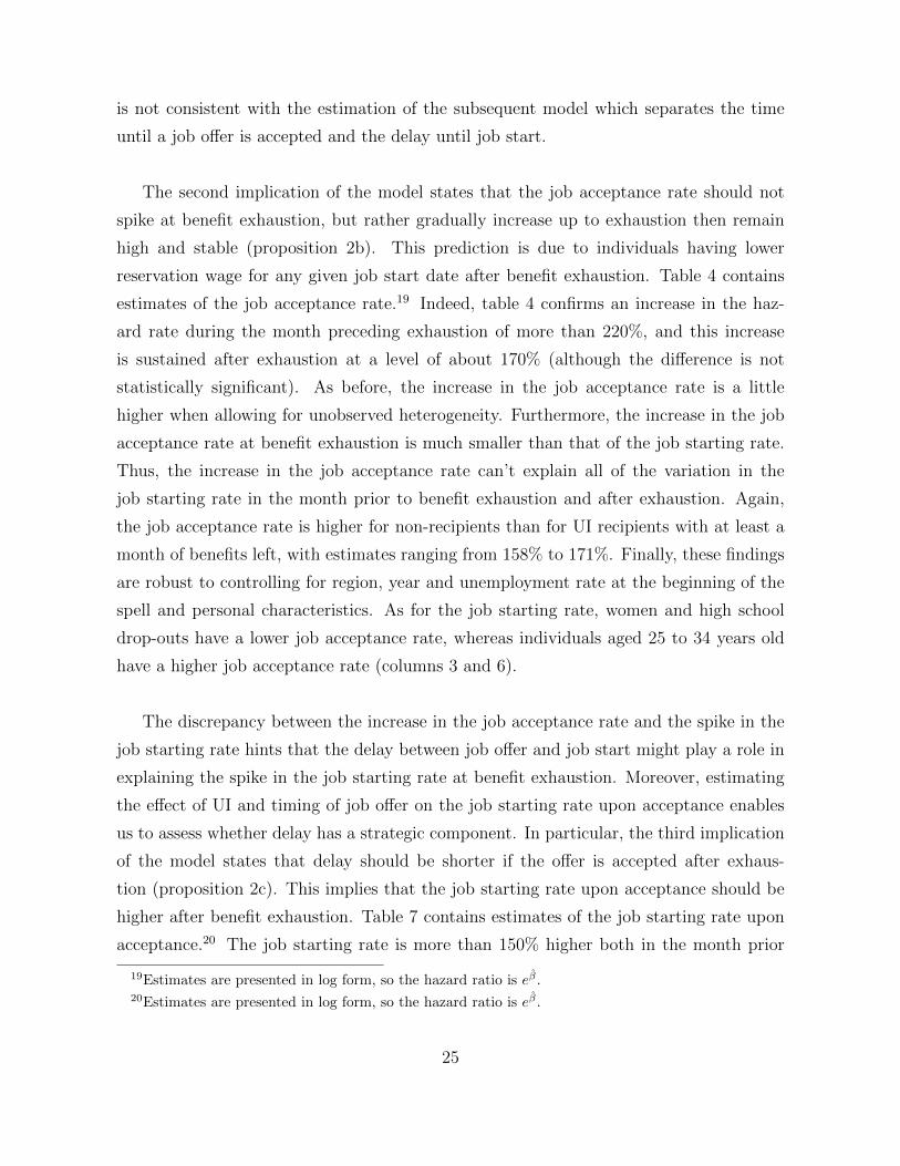
Further evidence of strategic delay is provided by figure 5, which shows the behaviour

of the job acceptance and job starting rate around benefit exhaustion.16 As suggested

16The hazard rates are computed as the number of individuals who exit a state in a given month divided

by the number of individuals remaining in that state at the beginning of the month, where the states are

respectively not having accepted an offer and not having started to work. In figure 5, the horizontal axis

denotes the time to exhaustion at the end of the month used for computation.

18

by the theoretical model, the job starting rate spikes at benefit exhaustion. Indeed, the

job starting rate more than doubles at exhaustion. The model also predicts that there

would be no spike in the job acceptance rate. However, this prediction is not validated

by the data, even though the spike in the job offer rate is much smaller than that in the

job starting rate (an increase of 15.7% compared to 111.8% for the job starting rate).

The fact that the job starting rate increases much more than the job acceptance rate at

benefit exhaustion suggests that individuals take advantage of UI benefits by strategi-

cally postponing job start after accepting an offer. While not shown in the figure, the

job starting rate among individuals with a pre-existing offer increases by 61% to reach

84% in the month prior to exhaustion (compared to an average monthly rate of 57% be-

fore exhaustion and 77% after exhaustion). Of course, the suggestive evidence presented

here do not account for differences in individuals characteristics, but the idea that delay

has a strategic component holds when including these differences in the empirical analysis.

4 Empirical Analysis

4.1 Methodology

Following the existing literature, I first estimate a reduced-form equation of the job start-

ing rate. Then I decompose the total duration of the jobless spell, ts, into two components,

the duration until a job offer is accepted, to, and the duration of delay between job offer

and job start, τ , and estimate a reduced-form equation for each of them.

For the purpose of the empirical analysis, each of the duration observed in the data

is assumed to come from a mixed proportional hazard model (MPH). The proportional

hazard (PH) model was first suggested by Cox (1972). This econometric model assumes

that the probability of leaving a state is affected proportionally by the covariates. The

MPH builds on the PH model by allowing for unobserved heterogeneity. The MPH was

introduced by Lancaster (1979) who applied it to unemployment duration. Lancaster

points out that not controlling for unobserved heterogeneity can lead to attenuation bias

and that it is especially important in the case of omitted variables or measurement errors.

Since our data set is particularly prone to measurement errors, allowing for unobserved

19

heterogeneity will have a large impact on the estimates. It is important to realize that this

analysis does not estimate the structural parameters of the model presented in section

2, and can’t distinguish between the job arrival rate and the job acceptance rate. More-

over, the proportional hazard model is not consistent with the theoretical model except

in some limited cases. This reduced-form analysis is nonetheless informative about the

determinants of delay and the role UI plays in it.

The first equation to be estimated is that of the job starting rate, i.e. the probability

that a job starts at time t, conditional on being unemployed at that time.17 This estima-

tion relates to the total duration of unemployment and is done solely for descriptive and

comparability purposes. This estimation is inconsistent with the subsequent estimation

of the sequential model. Following the literature, the job starting rate at duration t in

the jobless spell is assumed to be

θs(t|xs, us) = hs(t) exp(x′sβs)us (7)

where xs are observed characteristics at the beginning of the spell, us is the unobserved

heterogeneity with a distribution Gamma (1, σ) and hs is the time-dependence. Note

that us and xs are assumed to be independent. To allow for some flexibility, I assumed a

piecewise constant baseline hazard. I also included an indicator variable for being in the

month prior to benefit exhaustion and another for having exhausted the benefits. Thus,

the time-dependence can be written as

hs(t) = exp(∑k

µskImk(t) + γsIspike(t) + δsIexh(t)), (8)

where Imk is an indicator for being in the kth month since the beginning of the jobless

spell, Ispike(t) is an indicator for being in the month prior to exhaustion and Iexh(t) is an

indicator for having exhausted UI benefits. Note that Ispike(t) and Iexh(t) are identified

by the variation in UI benefit entitlement and take the nil value if the individual did not

receive UI during the spell. An indicator variable for receiving UI at some point during

the spell is included in the vector of observed characteristics.

17The literature typically uses the term “job finding rate” to refer to the rate at which individuals start

working. Since the goal of my paper is precisely to recognize that finding a job (i.e. accepting an offer)

differs from starting to work, I use the term “job starting rate”. Moreover, to avoid confusion with the

previous literature, I use“job acceptance rate” to refer to the rate at which individuals find a job.

20

The second equation to be estimated is that of the job acceptance rate, i.e. the

probability that a job offer is accepted at time t, conditional on not having accepted a

job offer before. The rate at which unemployed individuals accept job offers after being

jobless for a duration t is assumed to be

θo(t|xo, uo) = ho(t) exp(x′oβ)uo (9)

where xo are observed characteristics at the beginning of the spell, including an indicator

for receiving UI, uo is the unobserved heterogeneity with a distribution Gamma (1, σ)

and ho is the time-dependence. Again, uo and xo are assumed to be independent. The

baseline hazard is assumed piecewise constant and the time-dependence also includes an

indicator variable for being in the month prior to benefit exhaustion and another for

having exhausted the benefits. Thus, the time-dependence can be written as

ho(t) = exp(∑k

µokImk(t) + γoIspike(t) + δoIexh(t)), (10)

where Imk is an indicator for being in the kth month since the beginning of the jobless

spell, Ispike(t) is an indicator for being in the month prior to exhaustion and Iexh(t) is

an indicator for having exhausted UI benefits, both of which take the nil value for non-

recipients. Identification of the effect of benefit exhaustion and time effect is possible

because of the variability in the number of weeks of benefits. If all individuals had the

same length of benefit, it would be impossible to distinguish time-effect from exhaustion

effect.

The third equation to be estimated is that of the rate at which unemployed individuals

start working after having accepted a job offer, i.e. the probability that a job starts at a

duration τ after accepting a job offer, conditional on not having resumed work yet. The

job starting rate upon acceptance at duration τ is assumed to be

θ(τ |xτ , to, uτ ) = h(τ) exp(x′τβ + λto)uτ (11)

where to is the duration in unemployment until job offer, xτ are observed characteristics,

assumed independent from the unobserved heterogeneity, uτ ∼ Gamma (1, σ). The

baseline hazard is still assumed piecewise constant at the week level (rather than the

month in the case of the job acceptance rate). The time-dependence can then be defined

21

as

h(τ) = exp(∑k

µkIwk(τ) + γIspike(τ) + δIexh(τ)), (12)

where Iwk is an indicator for being in the kth week since the job was offered, Ispike(t) is an

indicator for being in the month prior to exhaustion and Iexh(t) is an indicator for having

exhausted UI benefits.

Observed characteristics controlled for vary from one specification to another. First,

all specifications include an indicator for not receiving UI benefits during the spell. There

are three other categories of control variables. The first set of regressors includes the

unemployment rate in the UI economic region, as well as province and year at the start of

the spell. Some specifications also include personal characteristics at the start of the spell:

age group, sex, family status (marital status and children), and highest level of education.

The last set of control variables, re-employment job characteristics, applies only to the

estimation of the job starting rate upon acceptance. It consists of a set of indicators for

being a union member, being employed in the public sector, and being employed in a large

firm (more than 500 employees). Some specifications also include occupation dummies to

control for the possibility that some jobs imply a long waiting period until job start (ex:

professors and teachers).

Furthermore, in the analysis of the delay between job offer and job start, the duration

of unemployment until job offer is included as a control in the form of a set of dummy vari-

ables indicating whether the offer was accepted within a month, within at least a month

and less than three months, within at least three months and less than six months. Not

controlling for the job offer time would likely bias upward the effect of exhausting benefits.

Effectively, the longer an individual has been unemployed at job offer, the less likely he

is to value delay before job start (assuming a decreasing marginal value of leisure), but

at the same time the longer an individual has been unemployed at job offer, the more

likely he has exhausted UI benefits. This creates an artificial correlation between benefit

exhaustion and delay if not controlling for time until job offer. However, for the time until

job offer to be exogenous, we need to make the restrictive assumption that the unobserved

heterogeneity uo and u are uncorrelated.

22

Some individuals have not accepted a job offer at the end of the period of observation

and are thus right-censored. Right-censoring is taken into account in the log likelihood

as follows

logL =N∑i=1

[cilogθ(ti|x) + logS(ti|x)], (13)

where t ∈ (ts, to, τ) is the completed duration or censoring time of the duration of in-

terest (subscripts denoting the type of duration are dropped for convenience), i is an

observation,ci indicates whether the duration is complete for observation i, and S(ti|x)

is the survivor function (probability that the duration lasts at least ti). The survivor

function can be written as

S(t|x) =

exp[−exp(x′β)∫ t

0h(s)ds] without unobserved heterogeneity

[1 + σ2exp(x′β)∫ t

0h(s)ds]−1/σ2

with u ∼ Γ(1, σ).(14)

However, there is no right-censoring in the estimation of the job starting rate upon ac-

ceptance, since whenever the offer date is observed, so is the job start date. Additionally,

individuals who dont accept an offer by the end of the survey period never begin the delay

duration, and are therefore excluded from the estimation of the job starting rate upon ac-

ceptance. The parameters of equations (7) to (11) are estimated by maximum-likelihood

using the above equations (13 and 14).

Another consideration is that more than a third of individuals have more than one

unemployment spell over the 6-year period of the panel. Thus, I allow for correlation

in the error terms by clustering the standard errors at individual level. However, the

unobserved heterogeneity is assumed uncorrelated across spells for the same individual.

The piecewise constant time-dependence is flexible and has been shown to be more

robust to assumptions about the distribution of the unobserved heterogeneity (Han and

Hausman (1990), Ridder (1987), Trussel and Richards (1985) ). Thus, even though the

unobserved heterogeneity is assumed to be gamma distributed, the results should remain

similar would another distribution be assumed. As a robustness check, I present results

from Cox regressions for all durations in the appendix (table A1). Cox regression is a non-

parametric method based on the rank and doesn’t make assumptions about heterogeneity.

23

However, it does not estimate the underlying baseline hazard, so it can’t be used to predict

the delay were UI benefits less generous. Finally, results from Probit regressions of the

probability of delaying more than two weeks are also presented in the appendix (table A2).

4.2 Results

The empirical analysis has two goals. First, it aims at testing the implications of the

theoretical model regarding the shape of the job acceptance and job starting rates around

benefit exhaustion. Second, it gives a first assessment of the determinants of delay be-

tween job offer and job start.

The first implication of the model states that the job starting rate should spike at

benefit exhaustion (proposition 2a). This prediction is due to individuals having a lower

reservation wage for jobs starting around exhaustion. Table 3 contains estimates of the

job starting rate.18 Indeed, table 3 reveals that the job starting rate is much higher in

the month preceding exhaustion. More precisely, without accounting for unobserved het-

erogeneity, the job starting rate increases by over 300% in the month prior to exhaustion,

but only by 200% after benefit exhaustion, creating a spike in the job starting rate before

benefit exhaustion (table 3, columns 1-3). Yet, not accounting for unobserved hetero-

geneity can lead to attenuation bias (Lancaster, 1990). When allowing for unobserved

heterogeneity, the magnitude of the estimated hazard ratio increases by more than 25%

both in the month prior to exhaustion and after exhaustion. However, although the job

starting rate remains higher in the month prior to exhaustion, it is not significantly higher

than that after exhaustion. Moreover, the job starting rate is higher for non-recipients

than for UI recipients with at least a month of benefits left. Estimates range from a job

starting rate 206% to 270% higher for non-recipients without and with unobserved het-

erogeneity respectively. The findings are robust to controlling for personal characteristics

(columns 3 and 6). Women and high school drop-outs have a lower job starting rate,

whereas individuals aged 25 to 34 years old have a higher job starting rate. Family status

and the unemployment rate at the beginning of the spell do not have much impact on the

job starting rate. This estimation replicates what has been done in previous studies and

18Estimates are presented in log form, so the hazard ratio is eβ .

24

is not consistent with the estimation of the subsequent model which separates the time

until a job offer is accepted and the delay until job start.

The second implication of the model states that the job acceptance rate should not

spike at benefit exhaustion, but rather gradually increase up to exhaustion then remain

high and stable (proposition 2b). This prediction is due to individuals having lower

reservation wage for any given job start date after benefit exhaustion. Table 4 contains

estimates of the job acceptance rate.19 Indeed, table 4 confirms an increase in the haz-

ard rate during the month preceding exhaustion of more than 220%, and this increase

is sustained after exhaustion at a level of about 170% (although the difference is not

statistically significant). As before, the increase in the job acceptance rate is a little

higher when allowing for unobserved heterogeneity. Furthermore, the increase in the job

acceptance rate at benefit exhaustion is much smaller than that of the job starting rate.

Thus, the increase in the job acceptance rate can’t explain all of the variation in the

job starting rate in the month prior to benefit exhaustion and after exhaustion. Again,

the job acceptance rate is higher for non-recipients than for UI recipients with at least a

month of benefits left, with estimates ranging from 158% to 171%. Finally, these findings

are robust to controlling for region, year and unemployment rate at the beginning of the

spell and personal characteristics. As for the job starting rate, women and high school

drop-outs have a lower job acceptance rate, whereas individuals aged 25 to 34 years old

have a higher job acceptance rate (columns 3 and 6).

The discrepancy between the increase in the job acceptance rate and the spike in the

job starting rate hints that the delay between job offer and job start might play a role in

explaining the spike in the job starting rate at benefit exhaustion. Moreover, estimating

the effect of UI and timing of job offer on the job starting rate upon acceptance enables

us to assess whether delay has a strategic component. In particular, the third implication

of the model states that delay should be shorter if the offer is accepted after exhaus-

tion (proposition 2c). This implies that the job starting rate upon acceptance should be

higher after benefit exhaustion. Table 7 contains estimates of the job starting rate upon

acceptance.20 The job starting rate is more than 150% higher both in the month prior

19Estimates are presented in log form, so the hazard ratio is eβ .20Estimates are presented in log form, so the hazard ratio is eβ .

25

to exhaustion and once the benefits are exhausted (table 5). Controlling for unobserved

heterogeneity increases the coefficient by about a third. These results imply that delays

are shorter if the offer is accepted near or after exhaustion, as predicted by the model.

Furthermore, the job starting rate conditional on having accepted a job offer is also much

higher for non-recipients than recipients with a least one month of benefits left. Besides,

the timing of job offer also matters for predicting the delay. Individuals who accepted

an offer in the first month of their jobless spell have a job starting rate upon acceptance

about 40% lower than those who accepted an offer later in their spell. This proportion

reaches 55% when including unobserved heterogeneity. Results are robust to controlling

for personal and re-employment job characteristics (columns 2 and 4), as well as occu-

pation (columns 3 and 6). The lower job starting rate for jobs offered early in the spell

could reflect either a decreasing marginal value of leisure or a credit constraint further in

the spell. In either case, it provides evidence that the delay between job offer and job

start has a strategic component.

On the other hand, part of the delay that could be qualified as institutional. In par-

ticular, re-employment job characteristics have an effect on the job starting rate upon

acceptance. In particular, jobs in the public sector are less likely to start quickly upon

acceptance,21 whereas unionized jobs are more likely to start quickly (not significant if

including unobserved heterogeneity). Moreover, single parents have a lower job starting

rate upon acceptance (significant only when including unobserved heterogeneity). A single

parent postponing job start could also be qualified as institutional delay if it takes time to

make childcare arrangements prior to starting a job. As a robustness check, results from

Cox regressions and Probit regressions of the probability of delaying more than two weeks

are presented in the appendix (table A1 and A2 respectively). Both the Cox regressions

and the Probit regressions support the idea that individuals receiving UI after accepting

a job offer postpone job start for a longer period.

21This finding is robust to excluding individuals in teaching occupations.

26

4.3 Cost of the delay

The empirical analysis showed that individuals substantially postpone job start after ac-

cepting job offer. This delay has a cost for the Unemployment Insurance program, since

benefits are paid until the job starts, sometimes long after the job is accepted. Table

6 presents the cost of delaying job start as a fraction of all benefits paid. The amount

of benefits paid to individuals still receiving UI while postponing job start accounts for

16.9% of all benefits paid. To compute this, I multiplied the weekly benefits by the num-

ber of weeks of UI benefits received after job offer, then summed it for all individuals and

divided by the total amount of benefits paid. If we do the same computation allowing for

an institutional delay of two weeks, then 10.7% of all benefits paid are paid to individuals

who delay in excess of the institutional threshold. Hence, the delay between job offer and

job start implies a large cost for the UI program even without accounting for the lost

income tax revenue for the government.

Of course, this estimates doesn’t control for differences in observed characteristics.

Using estimates from the survival analysis, I predict the delay as if UI were exhausted

for all individuals when accepting a job offer and, alternatively, as if all individuals were

non-recipients. Then, I compute the “excess” delay as the difference between the actual

delay and the predicted delay. Without unobserved heterogeneity, I find that about 8.2%

of all benefits paid are paid to individuals postponing job start after job offer in excess

than predicted had they exhausted their benefits before job offer. This fraction reaches

12.1% when taking unobserved heterogeneity into account. Similarly, without controlling

for heterogeneity, 8.5% of all benefits paid are paid to individuals postponing job start

in excess than predicted were they non-recipients. This proportion reaches 12.5% when

including unobserved heterogeneity. Therefore, the “excess” delay accounts for half to

three fourth of the total cost of delay (16.9% of all benefits paid). Although this cost

seems considerable, it could be mitigated by efficiency gains if receiving UI benefits en-

ables unemployed workers to accept better jobs starting later rather than accepting lower

paid jobs starting earlier. The following subsection test this hypothesis, as well as the

model prediction that wages and delay should be positively correlated for offers accepted

after exhaustion.

27

4.4 Efficiency gains

Postponing job start after job offer implies substantial costs for the UI program, and one

should be concerned that individuals receiving benefits strategically delay job start after

accepting a job offer. However, the overall cost might be much lower than estimated if

receiving UI enables unemployed workers to accept jobs that start later and are a better

match, rather than to accept the jobs that start the soonest. One way to assess the quality

of a match is by looking at the re-employment wage.

Table 7 contains regressions of the re-employment wage. There is a positive correlation

with the number of weeks between job offer and job start of an order of about 1%, and this

result is robust to including job characteristics and occupation (columns 1-3). However,

the positive relationship between wages and delay is driven by individuals who accepted

an offer after exhaustion and by non-recipients rather than by efficiency gains from re-

ceiving UI after accepting an offer. When interactions of delay and indicator variables for

accepting an offer after exhaustion and not receiving UI during the spell are included in

the model, the relationship between wages and delay disappears for those accepting an

offer before exhaustion (columns 4-6). Therefore, the possibility of postponing job start

while receiving UI benefits doesn’t lead to efficiency gains in terms of wages. However,

as predicted by the model, the effect of postponing job start on wages is positive (1.6%

to 2.5%) for non-recipients and for those accepting an offer after exhaustion. This result

supports the model’s prediction that wages and delay should be positively correlated for

offers accepted after benefit exhaustion and for non-recipients (proposition 2d). Intu-

itively, when individuals don’t receive benefits, they would rather start to work sooner

than later and will ask for a compensation to delay job start. To conclude, the analysis

of wages doesn’t support the hypothesis of efficiency gains from postponing job start, but

supports the prediction of a model in which individuals strategically postpone job start

to take advantage of the UI benefits.

4.5 Liquidity effect

The effect of Unemployment Insurance on the delay between job offer and job start could

be interpreted as a distortion in the marginal incentives or as a liquidity effect (Chetty,

28

2008). Intuitively, constrained individuals should be less inclined to delay than non-

constrained individuals other things being equal. When constrained, the marginal value

of consumption is higher than that of leisure, and delaying job start is less desirable.

Table 8 presents the average delay for different indicators of liquidity constraint. Follow-

ing Chetty(2008) and Krueger and Mueller(2010), I define an individual to be liquidity

constrained if either his earnings are below the low-income margin, has a mortgage or is

the single earner of the household. Overall, liquidity constrained individuals start to work

0.5 weeks before unconstrained individuals upon finding a job. This gap is a little smaller

if we look at the average for each indicator separately. The striking result of table 8 is

that the difference between constrained and unconstrained individuals is mostly driven by

those who accepted an offer before exhaustion. If Unemployment Insurance were affecting

the delay through a liquidity effect, it should have a larger impact on liquidity constrained

individuals and receiving UI should not change the average delay for unconstrained indi-

viduals. Yet, the difference between individuals who received UI benefits after accepting

an offer and those who didn’t is larger for unconstrained individuals. The findings are

very similar if we look at the fraction who delay at least two weeks.

The cumulative distribution of the delay by liquidity constraint (figure 6) shows that

the distribution of the delay is very similar for both liquidity constrained and uncon-

strained individuals who don’t receive UI benefits after accepting a job. However, liquid-

ity constrained individuals who receives benefits after accepting the job offer are more

likely to work at any duration after accepting a job than unconstrained individuals. This

suggests that moral hazard might be more important than liquidity effect in explaining

the correlation between the delay and Unemployment Insurance.

Table 9 shows the estimated parameters of the job starting rate by liquidity constraint.

The point estimates for constrained and unconstrained subsamples are not statistically

different. This finding confirms that the liquidity effect is not driving the relationship

between UI and delay, but rather that UI changes the marginal incentives to return to

work by providing a subsidy to delay job start.

29

5 Conclusion

Unemployment Insurance can alter job search behaviour and lead to longer unemployment

spells. The effect of UI on unemployment duration has been extensively documented, but

traditionally, it was assumed to be caused by an increase in the duration until a job offer

is accepted. This paper suggests that this is only part of the story. UI also affects another

component of the unemployment spell: the delay between job offer and job start.

In this paper, I developed a theoretical model where firms make job offers that in-

clude a wage and a start date. In this model, UI recipients are indifferent between a job

start now at a higher wage or a job start later at a lower wage but which enables them

to enjoy leisure subsidized by UI benefits. Once the benefits are exhausted, they would

rather start working now, and will accept a job that starts later only if the wage is high

enough to compensate for lost income while waiting for the job to start. Indeed, in the

data, longer delays are correlated with higher wages only for those who accepted an offer

after benefit exhaustion and for non-recipients. The model predicts that delay would be

longer on average for individuals accepting an offer before benefit exhaustion, which is

confirmed by the data. The model also rationalizes the empirical finding of a spike in the

job starting rate at benefit exhaustion, as suggested by Boone and Van Ours (2009). The

model predicts that the rate at which job offers are accepted increases until exhaustion

and remains stable thereafter. Thus, it can’t account for the empirical finding of a small

spike in the job offer rate. However, since the spike in the job starting rate is much more

pronounced than that in the job acceptance rate, the delay between job offer and job start

can explain at least part of the spike in the job starting rate.

The main contribution of this paper is to document the behaviour of postponing job

start after accepting a job offer, which has not been studied before. I find that individuals

who accepted an offer before benefit exhaustion delay job start by 3.9 weeks on average,

whereas the average delay is respectively 1.8 and 2.3 weeks for those who accepted a

job after exhaustion and those who did not receive benefits. Moreover, 54% of individu-

als with an offer accepted prior to exhaustion postpone job start by at least two weeks,

compared to 35% and 40% for those with an offer after exhaustion and non-recipients

respectively. Overall, this implies that 17% of all benefits paid are paid to individuals

30

who have already found a job, but have not started working yet. Moreover, half to three

quarters of the cost of delaying job start is due to delay in excess of the predicted delay

were the benefits exhausted at job offer or were the individuals not receiving UI at all.

Although no causal effect can be formally identified, this at least suggests that the delay

between job offer and job start is not solely driven by the employer side; rather some

individuals take advantage of the availability of benefits to postpone job start.

The empirical analysis also studied the determinants of delay. Receiving benefits

has a large negative impact on the job starting rate upon accepting a job. Although

no causal effect is identified, it supports the idea that individuals strategically postpone

job start. Similarly, the timing of job offer matters: accepting a job offer early in the

spell decreases the job starting rate upon acceptance. This finding could reflect either

a decreasing marginal value of leisure or it could reflect a credit constraint as the spell

progresses. In both cases, postponing job start would be less valuable further in the spell.

In any case, the effect of the timing of job offer on the job starting rate provides further

evidence that the delay between job offer and job start has a strategic component. How-

ever, personal characteristics such as age and gender don’t seem to affect the job starting

rate upon acceptance. Education has a non-monotonic effect and this effect varies across

specifications. In some specifications, single parents have a lower job starting rate upon

acceptance, which could be due to institutional constraints such as arranging for child-

care. Another evidence of the presence of an institutional delay is that re-employment

job characteristics are correlated with the job starting rate upon acceptance. Jobs in the

public sector are less likely to start quickly after the offer, whereas unionized jobs are

more likely to start quickly in some specifications.

Even though the cost implied by postponing job start is considerably high, the cost

could be mitigated by efficiency gains. For example, receiving UI could enable unem-

ployed workers to accept a better job that starts later by providing a subsidy during the

waiting period. Yet, this hypothesis is not supported by the regressions of wage on the

delay between job offer and job start. In particular, there is a positive correlation be-

tween wages and delay, but only for those who accepted the offer after benefit exhaustion

and for non-recipients, but not for individuals who still receive UI benefits after they ac-

cepted the offer. Furthermore, this result confirms the model prediction that wages should

31

be positively correlated with delay for jobs offered after exhaustion and for non-recipients.

Finally, the effect of Unemployment Insurance on the delay between job offer and job

start is larger for individuals who are not liquidity constrained, suggesting that UI distorts

the marginal incentives to resume work rather than acting through a liquidity effect.

Unfortunately, the data don’t allow to assess the effect of economic conditions on the

delay behaviour. Although there were fluctuations in the unemployment rate during the

period covered by the data, there was no recession in Canada during the 1993-2006 pe-

riod.22 Thus, one can hardly generalize the results to a deeper economic downturn, such

as the Great Recession in the United States. Consequently, even though I didn’t find a

statistically significant effect of the unemployment rate on the duration of the delay, it is

very possible that unemployed individuals resume work more quickly when offered a job

in an economic downturn, limiting the undesirable effects of UI benefits on unemployment

duration. Moreover, jobs accepted later in the spell are more likely to start quickly, sug-

gesting that the delay would be shorter during an economic downturn, when the job offer

arrival rate is low. Finally, if the length of the delay were to stay the same both in period

of economic growth and in recessions, the relative importance of the cost of delaying job

start would be mechanically much smaller in a period of recession, where the spells are

longer. Thus, the cost of the delay between job offer and job start should be more of a

concern in periods of expansion and might be negligible during deep economic downturns

like the Great Recession.

This paper is the first to study of the delay between job offer and job start. More

research has to be done in order to establish causal effects. Moreover, it will be important

to proceed to a structural estimation of the model’s parameters for policy simulation.

This will enable answering important questions such as how the government can improve

the UI system to make it less prone to strategic delay. It would also be interesting to look

at the efficiency gains of postponing job start for the employers. Do firms post vacancies

early to ensure a good match? Do they try to get their share of the pie by offering a lower

wage to UI recipients who would like to postpone job start?

22Only a reduced growth (below 2% in 1996, 2001 and 2003)

32

References

[1] James W. Albrecht and Bo Axell. An equilibrium model of search unemployment. The Journal ofPolitical Economy, 92(5):pp. 824–840, 1984.

[2] Gerard J. Van Den Berg. Nonstationarity in job search theory. The Review of Economic Studies,57(2):255–277, 1990.

[3] David M. Blau. Search for nonwage job characteristics: A test of the reservation wage hypothesis.Journal of Labor Economics, 9(2):pp. 186–205, 1991.

[4] David Card, Raj Chetty, and Andrea Weber. The spike at benefit exhaustion: Leaving the unem-ployment system or starting a new job? American Economic Review, 97(2):113–118, 2007. Morecomplete version http://www.nber.org/papers/w12893.pdf.

[5] David Card and Phillip B. Levine. Extended benefits and the duration of ui spells: evidence fromthe new jersey extended benefit program. Journal of Public Economics, 78(1-2):107–138, 2000.

[6] Raj Chetty. Moral hazard versus liquidity and optimal unemployment insurance. The Journal ofPolitical Economy, 116(2):173–234, 2008.

[7] D. R. Cox. Regression models and life-tables. Journal of the Royal Statistical Society. Series B(Methodological), 34(2):pp. 187–220, 1972.

[8] Peter A. Diamond. A model of price adjustment. Journal of Economic Theory, 3(2):156–168, 1971.

[9] Zvi Eckstein and Kenneth I. Wolpin. Estimating a market equilibrium search model from panel dataon individuals. Econometrica, 58(4):783–808, 1990.

[10] Aaron Han and Jerry A. Hausman. Flexible parametric estimation of duration and competing riskmodels. Journal of Applied Econometrics, 5(1):1–28, 1990.

[11] Lawrence F. Katz and Bruce D. Meyer. The impact of the potential duration of unemploymentbenefits on the duration of unemployment. Journal of Public Economics, 41(1):45–72, February1990.

[12] Alan B. Krueger and Andreas Mueller. Job search and unemployment insurance: New evidence fromtime use data. Journal of Public Economics, 94(3-4):298 – 307, 2010.

[13] Rafael Lalive. How do extended benefits affect unemployment duration? a regression discontinuityapproach. Journal of Econometrics, 142(2):785–806, 2008.

[14] Rafael Lalive, Jan Van Ours, and Josef Zweimuller. How changes in financial incentives affect theduration of unemployment. Review of Economic Studies, 73(4):1009–1038, 2006.

[15] Tony Lancaster. Econometric methods for the duration of unemployment. Econometrica, 47(4):pp.939–956, 1979.

[16] Bruce D. Meyer. Unemployment insurance and unemployment spells. Econometrica, 58(4):757–782,1990.

[17] Robert Moffitt. Unemployment insurance and the distribution of unemployment spells. Journal ofEconometrics, 28(1):85–101, 1985.

[18] Dale T. Mortensen. Chapter 15 Job search and labor market analysis, volume Volume 2, pages849–919. Elsevier, 1986.

[19] Jan C van Ours and Milan Vodopivec. How shortening the potential duration of unemploymentbenefits affects the duration of unemployment: Evidence from a natural experiment. Journal ofLabor Economics, 24(2):351–378, 2006.

33

[20] Geert Ridder. The sensitivity of duration models to misspecified unobserved heterogeneity andduration dependence. 1987.

[21] Richard Rogerson, Robert Shimer, and Randall Wright. Search-theoretic models of the labor market:A survey. Journal of Economic Literature, 43(4):959–988, 2005.

[22] Andrew Shephard. Equilibrium search and tax credit reform, 2009.

[23] James Trussell and Toni Richards. Correcting for unmeasured heterogeneity in hazard models usingthe heckman - singer procedure. Sociological Methodology, 15:242–276, 1985.

[24] Gerard J. Van Den Berg. Empirical inference with equilibrium search models of the labour market.The Economic Journal, 109(456):283–306, 1999.

34

A Proofs

Proof. Proposition 1a. Case t ≥ T :

After exhaustion, the problem becomes stationary, so V u(t) = V u and V e(w(τ), τ, t) = V e(w(τ), τ).

Equations 2 and 3 respectively simplifiy to

V e(w, τ) =1− e−ρτ

ρu(b, lu)− e−ρτ

ρu(w, le)

and

V u =

∫ ∞t

[

∫ s

t

e−ρ(v−t)u(b, lu)dv + e−ρ(s−t)Ew,τ (max(V e(w, τ), V u)]dG(s; t)

=u(b, lu)

λ+ ρ+

λ

λ+ ρEw,τ (max(V e(w, τ), V u)

=u(b, lu)

ρ+λ

ρEw,τ (max(V e(w, τ)− V u, 0).

Worker is indifferent between accepting or rejecting a job if V e(w(τ), τ) = V u. Substituting usingthe equations above we get

1− e−ρτ

ρu(b, lu)− e−ρτ

ρu(τ) =

u(b, lu)

ρ+λ

ρEw,τ (max(V e(w, τ)− V u, 0)

where Ew,τ (max(V e(w, τ)− V u, 0)) can be rewritten as

∫ M

0

∫ u(W,le)

u(z)

(V e(w, z)− V e(w(z), z)dQ(u|z)dF2(z)

=

∫ M

0

∫ u(W,le)

u(z)

[(1− e−ρz

ρu(b, lu)− e−ρz

ρu(w, le))− (

1− e−ρz

ρu(b, lu)− e−ρz

ρu(z))]dQ(u|z)

=

∫ M

0

∫ u(W,le)

u(z)

e−ρz

ρ[u(w, le)− u(z)]dQ(u|z)dF2(z)

=

∫ M

0

∫ u(W,le)

u(z)

e−ρz

ρ(1−Q(u|z))dudF2(z) by integration by parts.

Plugging it in the previous equation and rearranging gives equation 4.(i) It is easy to see that u(τ) is strictly increasing in τ as long as ρ > 0.

b. Case t < T :Taking the derivative with respect to time of equation 3, we have

dV u(t)

dt= −u(B(t), lu)− λEw,τ (max(V e(w, τ, t)− V u, 0)) + ρV u(t)

Taking the derivative with respect to time of V u(t) = V e(w(τ), τ, t), we have

dV u(t)

dt= e−ρτu(B(t+ τ), lu)− u(B(t), lu) + ρ

∫ t+τ

t

e−ρ(v−t)u(B(v), lu)dv +e−ρτ

ρ

∂u(τ, t)

dt.

35

Equating the two equations above, rearranging and substituting using equation 3 gives

∂u(τ, t)

dt= ρu(τ, t)− ρu(B(t+ τ), lu)− λ ρ

e−ρτEw,τ (max(V e(w, τ, t)− V u, 0))

= ρu(τ, t)− ρu(B(t+ τ), lu)− λ ρ

e−ρτ

∫ M

0

∫ u(W,le)

u(z,t)

e−ρz

ρ[(1−Q(u|z))dudF2(z)]

by integration by parts (see a.)

(i) Define the u∗(τ, t) as the optimal reservation wage at time t if the environment remains stationaryafter t, i.e.

u∗(τ, t) ≡ u(B(t), lu) +λ

ρ

∫ M

0

∫ u(W,le)

u∗(z,t)

e−ρ(z−τ)(1−Q(u|z))dudF2(z)

For t < T , we have

u∗(τ, t)− λ

ρ

∫ M

0

∫ u(W,le)

u∗(z,t)

e−ρ(z−τ)(1−Q(u|z))dudF2(z) = u(B, lu)

> u(b, lu)

= u(τ, T )− λ

ρ

∫ M

0

∫ u(W,le)

u(z,T )

e−ρ(z−τ)(1−Q(u|z))dudF2(z).

Noting that x− λρ

∫M0

∫ u(W,le)

xe−ρ(z−τ)(1−Q(u|z))dudF2(z) is an increasing function of x, it implies that

u∗(τ, t) > u(τ, T ) for all t < T . The remaining of the proof follows the intuition of Van den Berg (1990).More precisely, the discrepancy between u∗(τ, t) and u(τ, t) arises only because of the anticipation of achange in the benefit level. As the exhaustion date approaches, the positive discounting and the decreasein the probability of finding a job before exhaustion increase the effect of the anticipation and, thus,increase the difference between u∗(τ, t) and u(τ, t). However, since the benefits are stationary before

exhaustion, u(τ, t) is the only variable that changes before exhaustion, so ∂u(τ,t)∂t increases in absolute

value (i.e. the sign of ∂2u(τ,t)∂t2 is the same as that of ∂u(τ,t)

∂t ). In particular, limt→T− u∗(τ, t) > u(τ, T )implies that the reservation utility is decreasing, and thus concave.

(ii) & (iii) Worker is indifferent between accepting or rejecting a job if V e(w(τ), τ, t) = V u(t). Derivingboth sides, we get

e−ρτu(B(t+ τ), lu)− e−ρτ u(τ, t)− e−ρτ

ρ

∂u(τ, t)

∂τ= 0

which can be rewritten∂u(τ, t)

∂τ= ρ[u(B(t+ τ), lu)− u(τ, t)].

The sign of the RHS of the equation depends on whether u(τ, t) is larger than u(B(t+ τ), lu). Notethat for τ ∈ [T − t], u(B(t + τ), lu) = u(b, lu) is smaller than the utility flow for any accepted offer(otherwise the offer would not be accepted), so the RHS is positive.

36

B Notation Summary

w ∈ [0,W ] wageτ ∈ [0,M ] delay between job offer and job startF1(w|τ) wage distribution conditional on delayF2(τ) probability distribution of delay between job offer and job startλ offer arrival ratet time elapsed since the beginning of unemployment spellto duration of unemployment spell at job offerts duration of unemployment spell at job startlt leisure in period tle leisure if employedlu leisure if unemployedl leisure schedule, i.e. l = (l1, l2, ..., lt, ...)ct consumption in period tc consumption schedule, i.e. c = (c1, c2, ..., ct, ...)B(t) consumption if unemployed in period tb home production and other source of income if UI benefits are exhaustedB home production and unemployment benefits if not exhaustedT benefit exhaustionρ worker subjective discount rateu(ct, lt) utility flow in period tU(c, l) Life-time utilityV e(w, τ, t) value of being employed in τ periods at wage w in period tV u(t) value of being unemployed in period tu(τ, t) reservation utility for a job start in τ periods in period tQ(u|τ) conditional distribution of utility flow once the job has startedw(τ, t) reservation wage for a job start in τ periods in period tθo(t) job acceptance rate (conditional on not having accepted a job before)θs(t) job starting rate in period t (conditional on not having started working yet)θτ (z) job starting rate conditional on having accepted a job offer z periods ago and not having started working yet

37

Figure 1: Distribution of jobless spell durations (completed spells)

Figure 2: Distribution of jobless spell durations at job offer (completed spells)

38

Figure 3: Distribution of delay between job offer and job start (completed spells)

Figure 4: Cumulative distribution of delay between job offer and job start (completed spells)

39

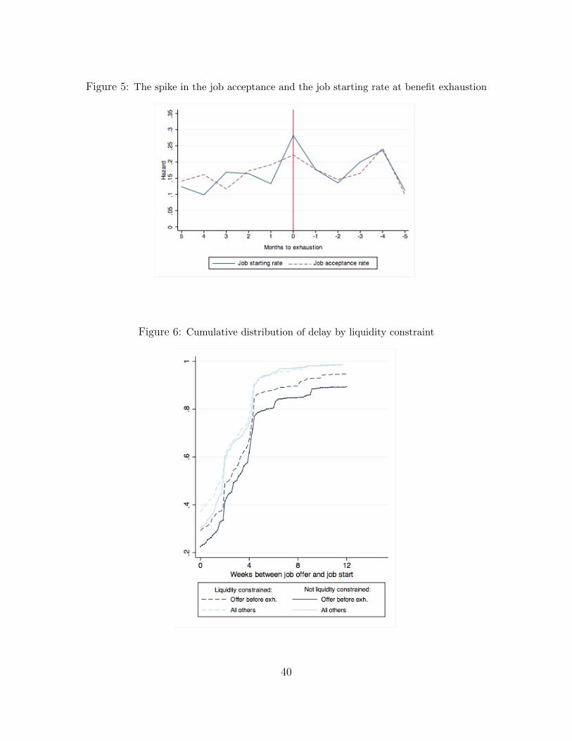
Figure 5: The spike in the job acceptance and the job starting rate at benefit exhaustion

Figure 6: Cumulative distribution of delay by liquidity constraint

40

Table 1: Delay for those who accepted the offer before exhaustion, after exhaustion andnon-recipients

Total Offer time<20 weeks ≥ 20 weeks

Mean delay between job offer and job start (weeks)Offer before exhaustion 3.9 4.5 2.7Offer after exhaustion 1.8 1.8Non-recipients 2.3 2.3 2.0Total 2.7 2.9 2.2

Fraction with delay longer than 2 weeksOffer before exhaustion 0.54 0.59 0.45Offer after exhaustion 0.35 0.35Non-recipients 0.40 0.42 0.35Total 0.44 0.46 0.36

Table 2: Mean of control variables and other selected variables

Offer before exhaustion Offer after exhaustion Non-recipients Right-censoredPersonal characteristics (at the beginning of the spell)Age 38.8 39.4 35.7 41.0Women 0.41 0.44 0.46 0.51Single without child 0.28 0.33 0.35 0.34Married without child 0.21 0.19 0.16 0.18Married with children 0.44 0.41 0.43 0.42Single parent 0.08 0.07 0.07 0.06Highschool drop-out 0.16 0.21 0.16 0.21Highschool graduate 0.32 0.27 0.32 0.29College graduate 0.07 0.04 0.11 0.09RegionAtlantic 0.23 0.21 0.10 0.15Quebec 0.37 0.18 0.24 0.23Ontario 0.25 0.38 0.37 0.38Prairies 0.10 0.11 0.17 0.14British Columbia 0.06 0.13 0.12 0.10Re-employment job characteristics (at job start)Union 0.24 0.18 0.16Public sector 0.09 0.08 0.08Large firm 0.21 0.27 0.23Wage 14.39 13.85 15.52Other characteristicsPrevious wage 14.61 15.19 15.12Observed spell length (weeks) 20.8 58.7 14.7 23.4Observations 5289 1161 8860 2191

41

Table 3: Mixed proportional hazard estimates - job starting rate

(1) (2) (3) (4) (5) (6)UI benefitsExhausted Benefits 0.7735*** 0.7877*** 0.7727*** 1.5702** 1.0767*** 1.1106***

(0.1288) (0.1240) (0.1191) (0.6632) (0.2738) (0.2660)< 1 month left 1.1611*** 1.1388*** 1.1131*** 1.7003*** 1.3706*** 1.3962***

(0.1711) (0.1702) (0.1673) (0.4360) (0.2568) (0.2833)Non-recipient 0.7213*** 0.7338*** 0.7611*** 0.9917*** 0.8660*** 0.9089***

(0.0593) (0.0577) (0.0568) (0.1389) (0.1038) (0.1060)Personal characteristics (at the beginning of the spell)20-24 years old 0.0143 0.0533

(0.1085) (0.1367)25-34 years old 0.2464*** 0.3296***

(0.0932) (0.1240)35-44 years old 0.0874 0.1409

(0.0952) (0.1215)45-54 years old 0.0846 0.1175

(0.1001) (0.1246)Women -0.2252*** -0.2508***

(0.0641) (0.0762)Married without child 0.0388 0.0562

(0.0761) (0.0920)Married with children -0.0485 -0.0371

(0.0784) (0.0952)Single parent -0.0565 -0.0761

(0.0936) (0.1184)High-school graduate 0.1740** 0.2151**

(0.0807) (0.1029)Some post-secondary 0.1438* 0.1705*

(0.0758) (0.0966)College graduate 0.2145* 0.2676*

(0.1225) (0.1539)Unemployment rate -0.0052 -0.0030 -0.0057 -0.0035

(0.0055) (0.0055) (0.0066) (0.0067)Unobserved heterogeneity No No No Gamma Gamma GammaLog σ2 -1.2708*** -1.8935*** -1.8162***

(0.3094) (0.4774) (0.4085)Region and year dummies No Yes Yes No Yes YesMonths in unemployment dummies Yes Yes Yes Yes Yes YesBIC 9.690e+07 9.534e+07 9.451e+07 9.646e+07 9.518e+07 9.430e+07Log-likelihood -4.845e+07 -4.767e+07 -4.725e+07 -4.823e+07 -4.759e+07 -4.715e+07Number of spells 17501 17501 17501 17501 17501 17501Number of completed spells 15310 15310 15310 15310 15310 15310

Notes: Log relative-hazard form. Significance level: *** 1% , ** 5%, *10%.Standard errors in parenthesis. σ2 is the variance of unobserved heterogeneity.

42

Table 4: Mixed proportional hazard estimates - job acceptance rate

(1) (2) (3) (4) (5) (6)UI benefitsExhausted Benefits 0.5274*** 0.5536*** 0.5357*** 0.7297*** 0.6272*** 0.6279***

(0.1303) (0.1244) (0.1218) (0.2375) (0.1737) (0.1791)< 1 month left 0.8303*** 0.8148*** 0.7975*** 0.9469*** 0.8574*** 0.8466***

(0.1741) (0.1721) (0.1684) (0.2296) (0.1860) (0.1864)Non-recipient 0.4584*** 0.4759*** 0.4955*** 0.5362*** 0.5058*** 0.5296***

(0.0660) (0.0633) (0.0609) (0.0909) (0.0807) (0.0806)Personal characteristics (at the beginning of the spell)20-24 years old 0.0835 0.0995

(0.1234) (0.1360)25-34 years old 0.2207** 0.2437**

(0.1094) (0.1215)35-44 years old 0.0843 0.0971

(0.1085) (0.1181)45-54 years old 0.1074 0.1186

(0.1197) (0.1297)Women -0.1472** -0.1513**

(0.0664) (0.0708)Married without child 0.0317 0.0373

(0.0825) (0.0886)Married with children -0.1037 -0.1033

(0.0777) (0.0836)Single parent -0.1307 -0.1353

(0.0984) (0.1058)High-school graduate 0.2112*** 0.2286***

(0.0788) (0.0855)Some post-secondary 0.1639** 0.1722**

(0.0750) (0.0825)College graduate 0.3081** 0.3363**

(0.1236) (0.1411)Unemployment rate -0.0064 -0.0037 -0.0063 -0.0034

(0.0060) (0.0060) (0.0063) (0.0064)Unobserved heterogeneity No No No Gamma Gamma GammaLog σ2 -2.0787*** -3.0294*** -2.9007***

(0.4885) (1.0398) (0.9361)Region and year dummies No Yes Yes No Yes YesMonths in unemployment dummies Yes Yes Yes Yes Yes YesBIC 7.666e+07 7.527e+07 7.473e+07 7.655e+07 7.525e+07 7.470e+07Log-likelihood -3.833e+07 -3.764e+07 -3.736e+07 -3.828e+07 -3.763e+07 -3.735e+07Number of spells 17501 17501 17501 17501 17501 17501Number of completed spells 15310 15310 15310 15310 15310 15310

Note: Log relative-hazard form. Significance level: *** 1% , ** 5%, *10%.Standard errors in parenthesis. σ2 is the variance of unobserved heterogeneity.

43

Table 5: Mixed proportional hazard estimates - job starting rate upon acceptance

(1) (2) (3) (4) (5) (6)UI benefitsExhausted Benefits 0.5913*** 0.4528*** 0.4384*** 0.7781*** 0.6451*** 0.6611***

(0.1011) (0.1099) (0.1125) (0.1439) (0.1591) (0.1678)< 1 month left 0.5802** 0.4583* 0.4972** 0.8423** 0.6899** 0.7355**

(0.2538) (0.2528) (0.2268) (0.3446) (0.3466) (0.3503)Non-recipient 0.4479*** 0.5213*** 0.5441*** 0.5348*** 0.7645*** 0.8478***

(0.0690) (0.0667) (0.0652) (0.0968) (0.1135) (0.1203)Job offer time (from the beginning of the unemployment spell)< 1 month -0.4769*** -0.4796*** -0.7703*** -0.8203***

(0.0708) (0.0709) (0.1195) (0.1228)[1-3) months 0.1414 0.1354 0.2408 0.2722

(0.1316) (0.1309) (0.2270) (0.2216)[3-6) months -0.0402 -0.0565 -0.1629 -0.2253

(0.1530) (0.1514) (0.2530) (0.2699)Re-employment job characteristics (at job start)Union 0.1785** 0.1653** 0.0948 0.0603

(0.0736) (0.0723) (0.1262) (0.1172)Public sector -0.3002*** -0.2744** -0.4014** -0.3030*

(0.1033) (0.1143) (0.1762) (0.1815)Large firm -0.0465 -0.0096 -0.0518 0.0291

(0.0759) (0.0737) (0.1257) (0.1256)Personal characteristics (at the beginning of the spell)20-24 years old 0.1398 0.1112 0.0127 -0.0398

(0.1357) (0.1340) (0.2210) (0.2245)25-34 years old -0.0611 -0.0758 -0.2108 -0.2420

(0.1185) (0.1171) (0.2022) (0.2011)35-44 years old -0.0677 -0.0433 -0.1897 -0.1680

(0.1208) (0.1208) (0.1947) (0.2053)45-54 years old -0.0113 -0.0388 -0.1327 -0.1769

(0.1185) (0.1189) (0.1966) (0.2085)Women -0.0040 -0.0150 0.0099 0.0172

(0.0641) (0.0672) (0.1026) (0.1116)Married without child 0.0395 0.0381 0.0073 0.0042

(0.0897) (0.0868) (0.1392) (0.1359)Married with children 0.0169 0.0163 -0.0371 -0.0534

(0.0842) (0.0816) (0.1300) (0.1313)Single parent -0.1462 -0.1695 -0.3758* -0.4491**

(0.1166) (0.1181) (0.2097) (0.2124)High-school graduate 0.1147 0.1181 0.2281* 0.2345*

(0.0871) (0.0873) (0.1380) (0.1401)Some post-secondary 0.1298 0.1431* 0.1580 0.1663

(0.0822) (0.0820) (0.1397) (0.1383)College graduate 0.0582 0.1301 0.0872 0.2635

(0.1402) (0.1478) (0.2484) (0.2679)Unemployment rate 0.0064 0.0080 0.0073 0.0123 0.0156 0.0169

(0.0065) (0.0063) (0.0064) (0.0096) (0.0099) (0.0103)Unobserved heterogeneity No No No Gamma Gamma GammaLog σ2 -1.0679*** -1.0355*** -0.8845***

(0.1156) (0.2066) (0.1171)Region and year dummies Yes Yes Yes Yes Yes YesWeeks since job offer dummies Yes Yes Yes Yes Yes YesOccupation dummies No No Yes No No YesBIC 1.192e+08 1.159e+08 1.151e+08 1.192e+08 1.148e+08 1.139e+08Log-likelihood -5.958e+07 -5.793e+07 -5.755e+07 -5.958e+07 -5.740e+07 -5.697e+07Number of completed spells 15310 15310 15310 15310 15310 15310

Note: Log relative-hazard form. Significance level: *** 1% , ** 5%, *10%.Standard errors in parenthesis. σ2 is the variance of unobserved heterogeneity.44

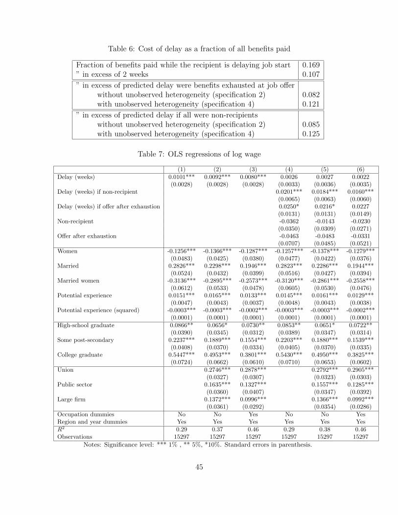
Table 6: Cost of delay as a fraction of all benefits paid

Fraction of benefits paid while the recipient is delaying job start 0.169” in excess of 2 weeks 0.107

” in excess of predicted delay were benefits exhausted at job offerwithout unobserved heterogeneity (specification 2) 0.082with unobserved heterogeneity (specification 4) 0.121

” in excess of predicted delay if all were non-recipientswithout unobserved heterogeneity (specification 2) 0.085with unobserved heterogeneity (specification 4) 0.125

Table 7: OLS regressions of log wage

(1) (2) (3) (4) (5) (6)Delay (weeks) 0.0101*** 0.0092*** 0.0080*** 0.0026 0.0027 0.0022

(0.0028) (0.0028) (0.0028) (0.0033) (0.0036) (0.0035)Delay (weeks) if non-recipient 0.0201*** 0.0184*** 0.0160***

(0.0065) (0.0063) (0.0060)Delay (weeks) if offer after exhaustion 0.0250* 0.0216* 0.0227

(0.0131) (0.0131) (0.0149)Non-recipient -0.0362 -0.0143 -0.0230

(0.0350) (0.0309) (0.0271)Offer after exhaustion -0.0463 -0.0483 -0.0331

(0.0707) (0.0485) (0.0521)Women -0.1256*** -0.1366*** -0.1287*** -0.1257*** -0.1378*** -0.1279***

(0.0483) (0.0425) (0.0380) (0.0477) (0.0422) (0.0376)Married 0.2826*** 0.2298*** 0.1946*** 0.2823*** 0.2286*** 0.1944***

(0.0524) (0.0432) (0.0399) (0.0516) (0.0427) (0.0394)Married women -0.3136*** -0.2895*** -0.2573*** -0.3120*** -0.2861*** -0.2558***

(0.0612) (0.0533) (0.0478) (0.0605) (0.0530) (0.0476)Potential experience 0.0151*** 0.0165*** 0.0133*** 0.0145*** 0.0161*** 0.0129***

(0.0047) (0.0043) (0.0037) (0.0048) (0.0043) (0.0038)Potential experience (squared) -0.0003*** -0.0003*** -0.0002*** -0.0003*** -0.0003*** -0.0002***

(0.0001) (0.0001) (0.0001) (0.0001) (0.0001) (0.0001)High-school graduate 0.0866** 0.0656* 0.0730** 0.0853** 0.0651* 0.0722**

(0.0390) (0.0345) (0.0312) (0.0389) (0.0347) (0.0314)Some post-secondary 0.2237*** 0.1889*** 0.1554*** 0.2203*** 0.1880*** 0.1539***

(0.0408) (0.0370) (0.0334) (0.0405) (0.0370) (0.0335)College graduate 0.5447*** 0.4953*** 0.3801*** 0.5430*** 0.4950*** 0.3825***

(0.0724) (0.0662) (0.0610) (0.0710) (0.0653) (0.0602)Union 0.2746*** 0.2878*** 0.2792*** 0.2905***

(0.0327) (0.0307) (0.0323) (0.0303)Public sector 0.1635*** 0.1327*** 0.1557*** 0.1285***

(0.0360) (0.0407) (0.0347) (0.0392)Large firm 0.1372*** 0.0996*** 0.1366*** 0.0992***

(0.0361) (0.0292) (0.0354) (0.0286)Occupation dummies No No Yes No No YesRegion and year dummies Yes Yes Yes Yes Yes YesR2 0.29 0.37 0.46 0.29 0.38 0.46Observations 15297 15297 15297 15297 15297 15297

Notes: Significance level: *** 1% , ** 5%, *10%. Standard errors in parenthesis.

45

Table 8: Mean delay by different indicator of liquidity constraint

Liquidity constrained Low-income Single earner MortgageNo Yes No Yes No Yes No Yes

Mean delay between job offer and job start (weeks)Offer before exhaustion 4.43 3.56 3.99 3.15 3.93 3.74 4.33 3.47Offer after exhaustion 2.07 1.72 1.83 1.85 1.79 1.95 1.94 1.55Non-recipients 2.38 2.20 2.27 2.18 2.30 2.12 2.19 2.28Total 3.05 2.54 2.76 2.42 2.76 2.55 2.83 2.57

Fraction with delay longer than 2 weeksOffer before exhaustion 0.58 0.51 0.55 0.47 0.54 0.52 0.56 0.51Offer after exhaustion 0.40 0.32 0.35 0.32 0.37 0.30 0.33 0.34Non-recipients 0.41 0.40 0.40 0.42 0.41 0.38 0.39 0.41Total 0.47 0.43 0.44 0.43 0.45 0.41 0.44 0.43

Table 9: Mixed proportional hazard estimates by liquidity - job starting rate upon acceptance

(1) (2) (3) (4) (5) (6)Liquidity constrainedExhausted Benefits 0.5203*** 0.5348*** 0.3790** 0.7188*** 0.7659*** 0.6636***

(0.1106) (0.1146) (0.1536) (0.1708) (0.1767) (0.2414)< 1 month 0.8423*** 0.8905*** 0.7455*** 1.2128*** 1.2433*** 1.1808**

(0.2438) (0.2346) (0.2444) (0.4479) (0.4615) (0.5160)Non-recipient 0.3786*** 0.3688*** 0.4736*** 0.4841*** 0.4718*** 0.9318***Completed spells 8011 8011 8011 8011 8011 8011

Not liquidity constrainedExhausted Benefits 0.6678*** 0.7016*** 0.6440*** 0.6897*** 0.8204*** 0.9106***

(0.1820) (0.1775) (0.2080) (0.2126) (0.2192) (0.2451)< 1 month 0.4109 0.4898 0.3219 0.4204 0.5663 0.4638

(0.3835) (0.3717) (0.3708) (0.4014) (0.4452) (0.4515)Non-recipient 0.5100*** 0.4945*** 0.5680*** 0.5236*** 0.5815*** 0.8917***

(0.1042) (0.0910) (0.0903) (0.1224) (0.1172) (0.1692)Completed spells 7299 7299 7299 7299 7299 7299Unobserved heterogeneity No No No Gamma Gamma GammaPersonal characteristics No Yes Yes No Yes YesJob characteristics No Yes Yes No Yes YesOccupation dummies No No Yes No No YesRegion and year dummies Yes Yes Yes Yes Yes YesWeeks since job offer dummies Yes Yes Yes Yes Yes Yes

Notes: Log relative-hazard form. Significance level: *** 1% , ** 5%, *10%. Standard errors inparenthesis.

46

Tab

leA

.1:

Cox

regr

essi

ons

Job

start

ing

rate

Job

acce

pta

nce

rate

Job

star

tin

gra

teu

pon

acce

pta

nce

(1)

(2)

(3)

(1)

(2)

(3)

(1)

(2)

(3)

(4)

UI

ben

efits

Exh

aust

edB

enefi

ts0.

9428

***

0.9

411***

0.9

161*

**0.6

627***

0.6

676

***

0.644

5***

0.465

5***

0.509

9***

0.39

00**

*0.

3815

***

(0.1

331)

(0.1

281

)(0

.121

9)(0

.1362)

(0.1

324)

(0.1

267)

(0.0

899)

(0.0

916

)(0

.095

4)

(0.0

984)

<1

mon

th1.

0789

***

1.0

622***

1.0

416*

**0.7

900***

0.7

819

***

0.767

0***

0.4

630*

*0.

4673*

*0.

349

1*0.3

809*

*(0

.163

5)(0

.1618

)(0

.160

5)(0

.1729)

(0.1

710)

(0.1

682)

(0.2

165)

(0.2

123

)(0

.210

6)

(0.1

890)

Non

-rec

ipie

nt

0.75

46***

0.7

658***

0.7

916*

**0.4

820***

0.4

973

***

0.515

1***

0.412

1***

0.404

9***

0.44

92**

*0.

4697

***

(0.0

597)

(0.0

585

)(0

.058

0)(0

.0667)

(0.0

647)

(0.0

629)

(0.0

640)

(0.0

601

)(0

.059

7)

(0.0

574)

Job

off

erti

me

(fro

mth

ebe

gin

nin

gof

the

un

emplo

ymen

tsp

ell)

<1

mon

th-0

.3480

***

-0.3

444*

**(0

.060

4)(0

.059

6)[1

-3)

mon

ths

0.04

71

0.04

44(0

.098

1)(0

.095

1)[3

-6)

mon

ths

-0.0

164

-0.0

206

(0.1

297)

(0.1

281)

Re-

emplo

ymen

tjo

bch

ara

cter

isti

cs(a

tjo

bst

art

)U

nio

n0.0

977

0.1

581*

*0.1

555*

*(0

.0661

)(0

.065

1)(0

.062

8)

Pu

bli

cse

ctor

-0.2

643*

**-0

.281

3**

*-0

.231

4**

(0.0

867

)(0

.088

5)(0

.093

4)

Lar

ge

firm

-0.0

509

-0.0

415

-0.0

187

(0.0

593

)(0

.061

7)(0

.059

3)

Per

son

al

chara

cter

isti

cs(a

tth

ebe

gin

nin

gof

the

spel

l)20

-24

yea

rsol

d0.0

220

0.0

984

0.1

273

0.12

110.

092

4(0

.1098

)(0

.125

0)

(0.1

121

)(0

.109

2)(0

.108

2)

25-3

4yea

rsol

d0.2

553

***

0.2

354**

-0.0

292

-0.0

198

-0.0

395

(0.0

944

)(0

.110

6)

(0.0

985

)(0

.094

6)(0

.093

4)

35-4

4yea

rsol

d0.0

957

0.1

033

-0.0

074

-0.0

287

-0.0

141

(0.0

968

)(0

.109

9)

(0.1

042

)(0

.098

4)(0

.097

9)

45-5

4yea

rsol

d0.0

847

0.1

206

0.0

025

0.00

54-0

.0192

(0.1

001

)(0

.119

9)

(0.1

005

)(0

.095

8)(0

.095

7)

Wom

en-0

.220

7***

-0.1

439*

*-0

.023

5-0

.0212

-0.0

333

(0.0

652

)(0

.067

2)

(0.0

523

)(0

.052

9)(0

.054

6)

Marr

ied

wit

hou

tch

ild

0.0

552

0.0

471

0.0

638

0.05

770.

052

7(0

.0775

)(0

.083

4)

(0.0

723

)(0

.071

5)(0

.067

7)

Marr

ied

wit

hch

ild

ren

-0.0

305

-0.0

908

0.0

196

0.01

430.

012

7(0

.0818

)(0

.079

8)

(0.0

693

)(0

.070

8)(0

.067

9)

Sin

gle

par

ent

-0.0

494

-0.1

275

-0.1

047

-0.1

147

-0.1

285

(0.0

963

)(0

.098

8)

(0.1

017

)(0

.104

9)(0

.105

3)

Hig

h-s

chool

grad

uat

e0.1

807

**0.2

112

***

0.0

929

0.11

060.

110

8(0

.0831

)(0

.079

5)

(0.0

773

)(0

.074

5)(0

.074

1)

Som

ep

ost-

seco

nd

ary

0.1

499

*0.1

662**

0.1

702

**0.

1561

**0.

1632

**(0

.0774

)(0

.076

0)

(0.0

709

)(0

.068

1)(0

.067

7)

Col

lege

grad

uat

e0.2

211

*0.3

150**

0.0

566

0.06

880.

112

6(0

.1259

)(0

.125

2)

(0.1

121

)(0

.111

8)(0

.114

1)

Un

emp

loym

ent

rate

-0.0

047

-0.0

024

-0.0

055

-0.0

028

0.00

320.

0035

0.00

51

0.00

50(0

.0055)

(0.0

056)

(0.0

060)

(0.0

060)

(0.0

060)

(0.0

057

)(0

.005

6)

(0.0

056)

Un

obse

rved

het

erog

enei

tyn

.a.

n.a

.n

.a.

n.a

.n

.a.

n.a

.n

.a.

n.a

.n

.a.

n.a

.R

egio

nan

dye

ard

um

mie

sN

oY

esY

esN

oY

esY

esN

oY

esY

esY

esO

ccu

pat

ion

du

mm

ies

No

No

No

No

No

No

No

No

No

Yes

BIC

2.742

e+05

2.7

36e+

05

2.7

31e+

05

2.1

56e

+05

2.15

1e+

05

2.1

48e

+05

2.6

21e

+05

2.668

e+05

2.6

64e+

052.6

64e+

05L

og-l

ikel

ihood

-1.3

71e+

05-1

.367e+

05

-1.3

64e+

05

-1.0

78e+

05-1

.075e

+05

-1.0

72e+

05-1

.310

e+05

-1.3

32e+

05-1

.330e

+05

-1.3

29e+

05N

um

ber

ofsp

ells

1750

117501

175

0117501

175

01

175

0117

501

1750

1175

0117

501

Nu

mb

erof

com

ple

ted

spel

ls15

310

15310

153

1015310

153

10

153

1015

310

1531

0153

1015

310

Log

rela

tive-

haza

rdfo

rm.

Sig

nifi

can

cele

vel:

***

1%,

**5%

,*1

0%.

Sta

nd

ard

erro

rsin

par

enth

esis

.

47

Table A.2: Probit regressions of the probability of delaying job start for at least two weeks

(1) (2) (3) (4)UI benefitsOffer after exhaustion -0.4840*** -0.4924*** -0.3900** -0.3848**

(0.1572) (0.1525) (0.1579) (0.1550)Non-recipient -0.3480*** -0.3531*** -0.4780*** -0.5235***

(0.0835) (0.0818) (0.0844) (0.0815)Job offer time (from the beginning of the unemployment spell)< 1 month 0.4657*** 0.4582***

(0.0901) (0.0873)[1,3) months -0.1338 -0.1513

(0.1291) (0.1264)[3,6) months 0.2473 0.2648

(0.1952) (0.1977)Re-employment job characteristics (at job start)Union 0.0033 -0.0599 -0.0215

(0.1098) (0.1058) (0.1027)Public sector 0.2039* 0.2304* 0.1565

(0.1232) (0.1219) (0.1209)Large firm 0.1192 0.0935 0.0423

(0.0956) (0.0964) (0.0913)Personal characteristics (at the beginning of the spell)20-24 years old 0.0396 0.0538 0.0741

(0.1532) (0.1552) (0.1531)25-34 years old 0.1680 0.1504 0.1565

(0.1299) (0.1295) (0.1284)35-44 years old 0.1947 0.2168 0.2055

(0.1339) (0.1325) (0.1312)45-54 years old 0.1982 0.2010 0.2306*

(0.1353) (0.1332) (0.1329)Women -0.0387 -0.0226 -0.0319

(0.0772) (0.0768) (0.0794)Married without child -0.1166 -0.1170 -0.1330

(0.1088) (0.1113) (0.1029)Married with children 0.0504 0.0481 0.0377

(0.1007) (0.1017) (0.0990)Single parent 0.2000 0.2107 0.2174

(0.1454) (0.1446) (0.1435)High-school graduate -0.1098 -0.1305 -0.1385

(0.1103) (0.1061) (0.1006)Some post-secondary -0.1111 -0.1110 -0.1267

(0.1077) (0.1052) (0.1017)College graduate -0.0024 -0.0331 -0.1492

(0.1615) (0.1624) (0.1588)Unemployment rate -0.0161** -0.0152** -0.0167** -0.0171**

(0.0075) (0.0074) (0.0074) (0.0074)Occupation dummies No No No YesRegion and year dummies Yes Yes Yes Yesbic 4.441e+07 4.394e+07 4.289e+07 4.203e+07ll -2.220e+07 -2.197e+07 -2.144e+07 -2.102e+07Number of spells (completed) 15310 15310 15310 15310

Standard errors in parenthesis. Significance level: *** 1% , ** 5%, *10%.

48