Financing Constraints and Corporate Investment

Basic Question

Is the impact of ‘finance’on ‘real’corporate investment fully summarized

by a price?

• cost of finance

• (user) cost of capital

• required rate of return

Or does (some) investment (additionally) depend on quantitative indicators

of the availability of finance?1

Motivation

Presence of significant financing constraints has potentially important im-

plications, e.g.

Business cycles - ‘financial accelerator’propagation mechanism

Monetary policy - ‘credit channel’transmission mechanism

Tax policy - effects of taxes on investment not summarized by effects on

user cost of capital

Takeovers - financial synergies

Assessment of ‘market-based’Vs ‘bank-based’financial systems

2

History

Offi cial inquiries: 1930 Macmillan Committee, 1979 Wilson Committee

Academic research:

Early empirical work on corporate investment stressed the availability of

finance (e.g. J.Meyer and E.Kuh, The Investment Decision: An Empirical

Study, 1957)

More or less forgotten for 30 years following Modigliani-Miller (AER 1958)

theorem

Revived interest in last 25 years, following influential empirical work by

Fazzari, Hubbard and Petersen (BPEA, 1988)

3

Intellectual respectability provided by development of theoretical models

of capital markets with asymmetric information (e.g. Stiglitz and Weiss,

AER 1981; Myers and Majluf, JFE 1984)

Although most of the empirical literature does not test any particular

model based on asymmetric information

Difference in cost of internal funds (retained profits) and external funds

(new equity or debt) needed for (some) investment to be ‘financially con-

strained’may reflect more mundane factors (e.g. transaction costs, differen-

tial taxes)

4

Definition

A firm’s investment is ‘financially constrained’if a ‘windfall’increase in

the availability of internal funds results in higher investment spending

A ‘windfall’change in the supply of internal funds is one which conveys no

new information about the profitability of current investment

5

Notice that this definition requires more than a positive correlation between

investment and indicators of the availability of internal funds

e.g. an increase in current profits may signal new information about future

profitability which justifies higher investment

Profits or cash flow may be correlated with investment even in the most

perfect of capital markets

This presents the main challenge in testing for the presence of financing

constraints

6

Note also that this definition does not require that firms are rationed in the

sense of Stiglitz and Weiss (AER 1981), or unable to raise external finance

at any price

It is suffi cient that, beyond some level, the firm faces a cost premium for

external finance, making external funds more expensive than internal funds

Such models tend to be called ‘pecking order’models in the corporate

finance literature (Myers, JF 1984), and ‘hierarchy of finance’models in the

economics literature (Hayashi, JPubE 1985)

7

Perfect capital markets

Investment is not financially constrained if firms can raise as much finance

as they desire at some exogenously given required rate of return

At least one source of external funds (new equity or debt) provides a perfect

substitute for internal finance from retained profits/cash flow

Financial policy is indeterminate

Only the cost of finance (required rate of return) influences the optimal

level of investment

8

Basic neoclassical factor demand model

• (shareholder) value-maximizing firms

• perfect capital markets

• no costs of adjusting the capital stock (up or down)

Firms undertake all positive NPV investment

First-order condition for optimal capital stock equates marginal product

of capital to user cost of capital (Jorgensen, AER 1963)

u ≈(pK

p

)(ρ + δ)

9

Given

•marginal product of capital (MPK)

• user cost of capital (u)

the availability of internal funds plays no role in the optimal investment

decision

〈Figures 1 and 2〉

NB. Drawn for a given level of the capital stock inherited from the previous

period (Kt−1) and capital accumulation equation Kt = (1− δ)Kt−1 + It, so

that there is a one-to-one correspondence between investment (It) and capital

stock in period t (Kt)10

Availability of internal funds (Ct) has no effect on the optimal level of

investment

[may affect whether any external funds are used (if desired investment

exceeds available internal funds)]

11

A simple pecking order model

• new equity is the only source of external finance

• issuing new equity imposes a cost, which increases with the amount of

new equity issued relative to the size of the firm

• formally, can think of this cost as a transaction fee paid to third parties

Required rate of return now depends on whether the marginal source of

finance is from (low cost) retained profits, or from (higher cost) new equity,

and on how much new equity is used

〈Figures 3 and 4〉

12

We now have two distinct financial regimes

Unconstrained regime:

Desired investment is less than available internal funds

No new equity is issued; firm pays positive dividends

Retained profits is the marginal source of finance

Constrained regime:

Desired investment exceeds available internal funds

New equity is issued; firm pays zero dividends

New equity is the marginal source of finance

13

For firms in the constrained regime, level of investment depends on the

amount of new equity issued, and therefore is sensitive to the availability of

internal funds

A ‘windfall’increase in cash flow (which here means no effect on MPK)

results in higher investment spending (Figure 4)

NB. The same firm is likely to be in different regimes at different times,

depending on the relative size of desired investment and available internal

funds

Introducing debt finance does not change these basic predictions, unless

debt provides a perfect substitute for internal funds

14

Towards empirical testing

The static demand for capital model, with costless adjustment, is too sim-

ple to be useful in empirical modelling

• since investment decisions can be costlessly reversed, only current condi-

tions matter

• expectations of future profitability play no role

• permanent and temporary increases in demand have the same effects on

current investment

15

To rationalize why current investment depends on expectations of future

profitability, we need to introduce some form of adjustment costs

To test the null hypothesis of no financing constraints, or perfect capital

markets, we then need to control for the effect of expected future profitability

on current investment decisions, and test for evidence of ‘excess sensitivity’

to fluctuations in the availability of internal funds

e.g. effects of cash flow on investment, holding constant expectations of

relevant future conditions

16

Ideally this requires a well-specified structural model that characterizes

dynamic capital stock adjustment, at least under the null of perfect capital

markets, and indicates how the influence of expected future conditions can

be controlled for

We don’t have such a model, except under very restrictive assumptions

Still it is useful to look at one of the leading models that has been proposed,

partly because it illustrates these issues, and partly because it is used inmuch

of the empirical literature

17

The Tobin-Hayashi Q model

• perfect competition

• constant returns to scale

• perfect capital markets

• symmetric and strictly convex (usually quadratic) adjustment costs

First-order condition for optimal investment equates marginal adjustment

cost (increasing in investment) to shadow value of an additional unit of

capital (or marginal q)

18

More formally, investment is chosen to maximize the value of equity

Vt = Et

{ ∞∑s=0

βs (Dt+s −Nt+s)

}where net distribution to shareholders is

Dt −Nt = Πt (Kt, It)

and net operating revenue is

Πt (Kt, It) = pt [F (Kt)−G (Kt, It)]− pKt It

and the capital accumulation equation is

Kt = (1− δ)Kt−1 + It

19

This can be written as a dynamic programming problem

Vt(Kt−1) =

{maxIt

Πt (Kt, It) + βEt [Vt+1 (Kt)]

}with first-order conditions

−(∂Πt

∂It

)= λKt

and

λKt =

(∂Πt

∂Kt

)+ (1− δ) βEt

[λKt+1

]where λKt =

(1

1−δ) (

∂Vt∂Kt−1

)is the shadow value of inheriting one additional

unit of capital in period t

20

Choosing a convenient functional form for adjustment costs

G (Kt, It) =b

2

[(I

K

)t

− a]2

Kt

we have (∂Πt

∂It

)= −pt

(∂G

∂It

)− pKt = −pt

(b

(I

K

)t

− ba)− pKt

and the foc for optimal investment can be written as(I

K

)t

= a +1

b

[((λKtpKt

)− 1

)pKtpt

]

= a +1

b

[(qt − 1)

pKtpt

]

21

The investment rate is a linear function of marginal qt =(λKtpKt

), the ratio

of the shadow value of an additional unit of capital to the purchase price of

an additional unit of capital

λKt =

(∂Πt

∂Kt

)+ (1− δ) βEt

[λKt+1

]= Et

{ ∞∑s=0

(1− δ)s βs(∂Πt+s

∂Kt+s

)}is the present value of current and expected future marginal revenue products

of capital

Marginal qt thus summarizes the impact of expected future conditions on

current investment decisions

22

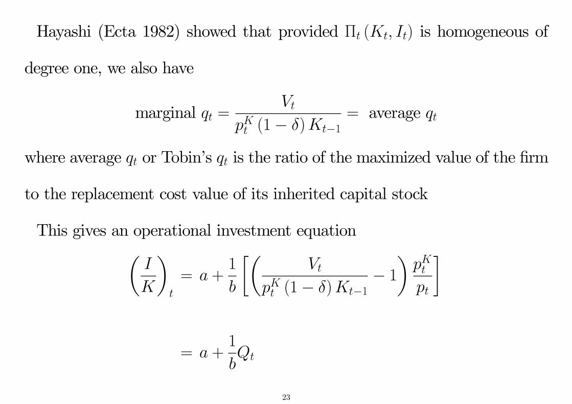
Hayashi (Ecta 1982) showed that provided Πt (Kt, It) is homogeneous of

degree one, we also have

marginal qt =Vt

pKt (1− δ)Kt−1= average qt

where average qt or Tobin’s qt is the ratio of the maximized value of the firm

to the replacement cost value of its inherited capital stock

This gives an operational investment equation(I

K

)t

= a +1

b

[(Vt

pKt (1− δ)Kt−1− 1

)pKtpt

]

= a +1

bQt

23

The usual empirical implementation further assumes that the maximized

value of the firm can be measured using the firm’s stock market valuation

(suitably adjusted for debt)

• which rules out bubbles, fads, or other share pricing anomalies

24

Excess sensitivity tests

If we maintain all the assumptions needed to derive the linear relation

between investment rates and average qt, we can then test the null hypothesis

of no financing constraints by adding additional financial variables to this

specification

Following FHP (1988), most studies add the ratio of cash flow to capital

stock (I

K

)t

= a +1

bQt + γ

(C

K

)t

and test the null hypothesis that γ = 0

25

(I

K

)t

= a +1

bQt + γ

(C

K

)t

This is motivated by the observation that, with a cost premium for external

finance, investment may also depend on the availability of internal funds, in

ways not fully captured by average qt

[This can be shown more formally; see Bond and Van Reenen (2007) for a

simple example]

But clearly this is a joint test of no financing constraints and all the other

(highly restrictive) assumptions of the Tobin-Hayashi Qmodel (perfect com-

petition, CRS, symmetric quadratic adj costs, no bubbles, ...)

26

Sample splitting tests

Recognizing that the baseline Q model may be mis-specified for other rea-

sons, FHP (1988) suggested investigating heterogeneity in the (excess) sen-

sitivity of investment to cash flow for sub-samples of firms with different

characteristics, that may be related to the cost premium for external finance

• sample splits may be based on dividend policy, credit rating, age, size,

growth, ownership, residence, ...

A variation uses sub-samples of firm-year observations with different char-

acteristics, that may be related to whether financing constraints are binding

• sample splits may be based on dividend payments, new share issues, ...27

This test would be most convincing if we could find

• one group of firms where we think the cost premium for external finance

is negligible, and not reject H0 : γ = 0 for that sub-sample

• another group of firms where we think the cost premium is significant,

and reject H0 : γ = 0 only for that sub-sample

Or if we could find

• one group of observations where we think financing constraints are not

binding, and not reject H0 : γ = 0 for that sub-sample

• another group of observations where we think financing constraints are

binding, and reject H0 : γ = 0 only for that sub-sample

28

Most empirical studies have not produced such clean results

The usual finding is that γ is positive and significant for all sub-samples,

but (significantly) bigger for sub-samples where firms may face a higher cost

premium for external funds (or where financing constraints are more likely

to be binding)

29

Motivated by the suggestion that investment-cash flow sensitivity is likely

to be greater when firms face a higher cost premium for external finance,

FHP (and many others) interpreted such evidence as being consistent with

financing constraints being important, and being more important for some

types of firms

e.g. those paying low or zero dividends, those without credit ratings,

younger or smaller firms, ...

〈Figure 5〉

30

Kaplan and Zingales (QJE 1997)

Kaplan and Zingales (1997) pointed out that investment-cash flow sensi-

tivity may not increase monotonically with the cost premium for external

finance

In a static demand for capital framework (no adjustment costs), the sen-

sitivity of investment to windfall fluctuations in the availability of internal

funds may be lower for firms with a higher cost premium for external funds,

if the marginal revenue product of capital is suffi ciently convex

〈Figure 6〉

31

Kaplan and Zingales (1997) concluded, rather forcefully, that investment-

cash flow sensitivities do not provide useful measures of the severity of fi-

nancing constraints

We can note two points here:

• this debate takes place under the alternative hypothesis that some, per-

haps most, firms face a non-negligible cost premium for external finance

• analyzing the simple correlation between investment and cash flow in a

static demand for capital model may tell us nothing at all about the

sensitivity of investment to cash flow conditional on measures of qt in

the presence of adjustment costs32

Curiously, the empirical work presented in Kaplan and Zingales (1997)

adopts the same augmented investment-average qt model used by FHP(I

K

)t

= a +1

bQt + γ

(C

K

)t

In fact, if we add a cost premium for external funds to the baseline Qmodel,

we can show that the conditional investment-cashflow sensitivitymeasured

by γ does increase monotonically with the cost premium for external finance

(Bond and Söderbom, JEEA 2013)

Although this result may be 15 years too late to overturn themis-perception

that Kaplan and Zingales (1997) proved the contrary

33

In my view the more serious concerns about the empirical literature on

financing constraints and corporate investment, in the tradition of FHP

(1988), are:

• controlling for measured average qt, cash flow may help to explain invest-

ment rates for reasons other than capital market imperfections

—and these reasons may be more important for some sub-samples than

for others

• very few studies have gone beyond rejecting the perfect capital markets

null hypothesis and tried to estimate structural investment models that

remain well-specified under the imperfect capital markets alternative

34

Other mis-specifications 1: share price bubbles

Even if the Tobin-Hayashi Q model is correctly specified, measurement of

average qt using stock market valuations may introduce highly persistent

measurement error in the presence of share price bubbles or fads

There may be no valid instruments to estimate the model consistently, if

the bubble component of the share price is itself correlated with relevant

information about fundamental values (Bond and Cummins, IFS WP, 2001)

35

Cummins, Hassett and Oliner (AER 2006) use analysts’earnings forecasts

and a simple valuation model to estimate fundamental values

They find that the resultingmeasure of average qt is muchmore informative

that the usual measure based on stock market valuations

And the coeffi cient on cash flow becomes insignificant, for all sub-samples

(see also Bond and Cummins, 2001; and Bond et al., 2004)

36

Other mis-specifications 2: market power

Hayashi (1982) showed that with imperfect competition (or decreasing re-

turns to scale), there is a wedge between marginal qt and average qt

Cooper and Ejarque (2003) show that this wedge is correlated with cash

flow, such that excess sensitivity to cash flow conditional on average qt may

reflect market power rather than capital market imperfections

37

Other null investment models

Excess sensitivity tests and sample splitting tests can be based on other

baseline models (valid under the null of no financing constraints) that require

less stringent assumptions than the Tobin-Hayashi Q model

For example:

i) marginal q models

• proposed by Abel and Blanchard (Ecta, 1986)

• used in this context by Gilchrist and Himmelberg (JME, 1995)

38

The basic idea is to estimate marginal qt from

λKt = Et

{ ∞∑s=0

(1− δ)s βs(∂Πt+s

∂Kt+s

)}by

• specifying a form for the marginal revenue product of capital

• using econometric forecasts of future values, discounted back to period t

This does not use share price data, and in principle can relax the assump-

tion of perfect competition

But measurement error in these estimates of marginal qt may also be severe

39

ii) Euler equation models

• proposed by Abel (1980)

• used in this context byWhited (JF, 1992), Bond and Meghir (RES, 1994)

Using

−(∂Πt

∂It

)= λKt

if we specify a form for marginal adjustment costs, we can eliminate λKt and

Et[λKt+1] from the intertemporal condition

λKt =

(∂Πt

∂Kt

)+ (1− δ) βEt

[λKt+1

]and estimate this ‘Euler equation’directly

40

• This also requires a form for the marginal revenue product of capital to

be specified

• But does not require an auxiliary forecasting model

This does not use share price data, and in principle can relax the assump-

tion of perfect competition

But still relies heavily on correct specification of adjustment costs

41

[More recent empirical work on corporate investment finds evidence for

non-convex forms of adjustment costs, e.g. (partial) irreversibility or fixed

costs, in addition to convex costs, which do not yield such convenient Euler

equations

See, for example, Doms and Dunne, REDy 1998; Cooper and Haltiwanger,

RES 2006; Bloom, Bond and Van Reenen, RES 2007; Bloom, Ecta 2009]

42

Structural investment models with imperfect capital markets

i) Hennessy, Levy and Whited (JFE, 2007)

With an increasing cost premium for new equity (and no debt finance),

obtain a structural investment equation that relates investment rates to

• average qt

• an interaction term between average qt and new share issues

Note that the interaction term is only relevant for firms in the constrained

regime, since unconstrained firms do not issue new shares

Extension to (costly) debt finance gives a similar model in terms of mar-

ginal qt, but can’t replace marginal qt by average qt with their specification43

ii) Bond and Söderbom (JEEA, 2013)

Similar model to Hennessy, Levy and Whited (JFE, 2007), but find a

specification with costly debt finance that does yield a structural investment

model, with (conventional) average qt and a similar interaction term

Not however implemented with real data

44

iii) Hennessy and Whited (JF, 2007)

Estimation of a fully parametric structural model with cost premia for

external funds, using simulated method of moments

Requires complete specification of the structural model (revenue function,

adjustment costs, stochastic shocks, cost premia, ...) such that model can

be simulated using numerical dynamic programming

Parameters estimated by matching features of simulated data to corre-

sponding features of empirical data (SMM)

45

State of the art in this literature, and promising direction for future re-

search

Although a concern with this approach (here and elsewhere) is that baseline

models are specified so parsimoniously, and fit so poorly, that any additional

parameters (reflecting cost premia for external finance, more complex adjust-

ment costs, ...) are likely to help to match some moments in the empirical

data (and hence appear to be highly significant)

46

Quasi-experimental evidence

The recent financial crisis (or crises) has prompted renewed interest in this

topic (particularly within central banks and financial regulators), and pro-

vided a (quasi-) experiment which may offer a more compelling identification

strategy

The basic idea is as follows:

- Divide banks into those whose balance sheets were affected more or less

severely by the financial crisis (objectivemeasures include credit default swap

rates, stock market capitalisation of banks, those which had to be rescued,

...)

47

- Divide (small) firms into those which - in the period before the crisis -

borrowed from the banks which were (subsequently) hit more or less severely

by the crisis

- Investigate whether investment spending during or after the crisis fell by

more for the firms which previously borrowed from the worst affected banks

than for the firms which previously borrowed from the least affected banks

Such a pattern would suggest that bank balance sheet weakness is passed

on to corporate borrowers, either through a higher cost of borrowing or re-

stricted availability of credit, and that (small) firms cannot easily substitute

other sources of external finance for bank loans

48

References:

Cingano, Manaresi, Sette, Review of Financial Studies, 2016

Franklin, Rostom, Thwaites, BoE StaffWorking Paper no. 557, 2015

Evidence from Italy and the UK suggests this bank balance sheet channel

did affect investment spending by smaller firms who (often) have a borrowing

relationship with a single bank

[Caveat: firms not randomly allocated to banks in the pre-crisis period;

banks which (e.g.) specialise in lending to construction firms may have been

hit particularly severely by the crisis, while investment by construction firms

may have fallen for reasons other than the cost or availability of credit]

49

Also less clear that this channel is important for larger corporations who

can borrow from multiple banks, or issue bonds or equity

Hence not clear how important this factor is in explaining the persistent

weakness of aggregate corporate investment in the period following the fi-

nancial crisis

50