financial shocks, firm credit and the great recession
TRANSCRIPT

Financial Shocks, Firm Credit and the Great RecessionNeil Mehrotra and Dmitriy SergeyevJanuary 2020

ARTICLE IN PRESSJID: MONEC [m3Gsc; February 12, 2020;3:33 ]
Journal of Monetary Economics xxx (xxxx) xxx
Contents lists available at ScienceDirect
Journal of Monetary Economics
journal homepage: www.elsevier.com/locate/jmoneco
Financial shocks, firm credit and the Great Recession
�
Neil Mehrotra
a , Dmitriy Sergeyev
b , ∗
a Federal Reserve Bank of New York, United Statesb Department of Economics, Bocconi University, via Rontgen 1, Milano, MI, 20135, Italy
a r t i c l e i n f o
Article history:
Received 30 July 2018
Revised 29 December 2019
Accepted 22 January 2020
Available online xxx
JEL classification:
E44
J60
Keywords:
Job flows
Financial frictions
Great Recession
a b s t r a c t
The creation and destruction margins of employment (job flows) can be used to measure
the employment effects of disruptions to firm credit. Using a firm dynamics model, we
establish that a tightening of credit to firms reduces employment primarily by reducing
gross job creation, exhibiting stronger effects at new, young, and middle-sized firms. The
firm credit channel accounts for, at most, 18%, of the decline in US employment in the
Great Recession. Using MSA-level job flows data, we show that the job flows response to
identified credit shocks is consistent with our model’s predictions.
© 2020 Elsevier B.V. All rights reserved.
1. Introduction
During the Great Recession, employment decreased approximately 6% from its peak in late 2007 to its trough in early
2010. 1 The sharp decline in US employment and its slow recovery have prompted an extensive debate on the underlying
causes of the Great Recession and the channels through which a financial crisis reduces employment. In particular, the rel-
ative importance of competing channels through which the financial crisis reduced employment remains an open question.
Narratives and models of the Great Recession emphasize a variety of channels through which the financial crisis lowered
employment. One prominent view emphasizes the demand effects of household deleveraging: falling house prices reduce
� The views expressed herein are the views of the authors and do not necessarily represent the views of the Federal Reserve Bank of New York or the
Federal Reserve System. This version follows a previous version of this paper circulated as “Financial Shocks and Job Flows.” We would like to thank Gian
Luca Clementi, John Cochrane, Steve Davis, Gauti Eggertsson, Simon Gilchrist, Joao Gomes, John Haltiwanger, Erik Hurst, Pat Kehoe, Guido Menzio, Simon
Mongey, Andreas Mueller, Emi Nakamura, Ali Ozdagli, Nicola Pavoni, Ricardo Reis, Jose Victor Rios Rull, Jón Steinsson, Guido Tabellini, Gianluca Violante,
and Mike Woodford for helpful discussions and seminar participants at Bocconi University, Brown University, Columbia University, Federal Reserve Bank of
Minneapolis, Federal Reserve Bank of New York, LUISS, NYU, Toulouse School of Economics, University of Maryland; 2014 NBER ME Program Meeting, 2016
NBER EF&G Research Meeting, Midwest Macro Meetings, North American Summer Meeting of the Econometric Society, the Boston Fed/BU Macro-Finance
Linkages Conferences, ESSIM for their comments. Neil Mehrotra thanks the Ewing Marion Kauffman Foundation for financial support through the Kauffman
Dissertation Fellowship.∗ Corresponding author.
E-mail address: [email protected] (D. Sergeyev).1 Seasonally adjusted total nonfarm employment is taken from the US Bureau of Labor Statistics. The peak is in December 2007 and the trough is in
January 2010.
https://doi.org/10.1016/j.jmoneco.2020.01.008
0304-3932/© 2020 Elsevier B.V. All rights reserved.
Please cite this article as: N. Mehrotra and D. Sergeyev, Financial shocks, firm credit and the Great Recession, Journal of
Monetary Economics, https://doi.org/10.1016/j.jmoneco.2020.01.008

2 N. Mehrotra and D. Sergeyev / Journal of Monetary Economics xxx (xxxx) xxx
ARTICLE IN PRESS
JID: MONEC [m3Gsc; February 12, 2020;3:33 ]
household consumption interacting with wage/price rigidities and the zero lower bound to reduce employment. 2 A second
view has emphasized disruptions to the flow of new credit to firms that impeded business expansion and investment. 3 A
third channel emphasizes higher discount rates (risk premia, etc.) which reduce hiring and physical investment at firms
while shifting household asset demand towards risk-free assets. 4 While hardly exhaustive, this taxonomy is useful in think-
ing through distinct channels by which firms are induced to shed workers. Though it is likely that each channel played some
role, the importance of each of these mechanisms remains debated.
In this paper, we argue that gross job flows can help separate and quantify these channels, with a particular emphasis on
the contribution of the firm credit channel. 5 Our main finding is that the firm credit channel contributed, at most, only 18%
to the decline in employment during the Great Recession. By contrast, in models with a representative firm subject to fi-
nancial frictions, this channel typically accounts for all of the decline in employment. 6 Our decomposition instead attributes
most of the decline in employment (58%) to what is labeled as the discount rate shock, providing support for narratives of
the Great Recession that emphasize macrofinance channels: rising risk premia, increased pessimism, or heightened percep-
tions of uncertainty. This finding is driven by the empirical fact that employment is concentrated at large and mature firms
and, while there is a differential sensitivity of job flows across firm age and size in the 2008 recession, these differences
are not strong enough to favor financial shocks over shocks that carry a more uniform effect across the firm age and size
distribution.
It is worth emphasizing that our conclusion is not that the financial crisis only accounts for 18% of the decline in em-
ployment, but, rather, that the channel of credit disruption to firms accounts for only 18% of the decline in employment.
The financial crisis rather affected employment via demand and risk premia channels.
We begin by illustrating qualitatively how a disruption to firm credit decreases employment primarily by reducing gross
job creation. In contrast, it can be shown theoretically that a household credit disruption that lowers consumer demand
or a financial panic that operates indirectly through elevated risk premia decreases employment primarily by raising job
destruction.
Next, we show how overall job flows and flows by firm age/size can disentangle the relative contribution of these chan-
nels. A calibrated firm dynamics model is used to quantify the contribution of each channel to the overall decline in US
employment. Our calibrated model matches a wide range of moments of the distribution of employment by firm age and
size. Importantly, only a small fraction of firms in our model are financially constrained in accordance with evidence that
the aggregate balance sheet of nonfinancial US firms was quite healthy throughout the Great Recession.
To model job flows, one must move away from a representative firm to an environment with expanding firms (con-
tributing to gross job creation) and contracting firms (contributing to gross job destruction). The difference between gross
job creation and gross job destruction is the change in employment. Fig. 1 shows the behavior of gross job flows during the
Great Recession. To our knowledge, our paper is the first to theoretically model how gross job flows respond to different
business cycle shocks and utilize these differences to help identify the type of shocks at work. 7
The financial shock is modeled as a tightening of financial constraints in a firm dynamics model with financial frictions
and decreasing returns to scale production. 8 Newly born firms and young firms accumulate assets and expand towards
their optimal scale. Mature firms are more likely to be financially unconstrained and are free to expand or contract subject
to idiosyncratic shocks to firm productivity or changes in factor prices. Firms differ in productivity levels so that some
businesses remain small without any binding financial constraint. In our calibration, most financially constrained firms are
small/medium-sized firms, but the vast majority of small/medium-sized firms are not constrained. 9
In addition to a financial shock, our model includes a productivity shock and a discount rate shock that forms a wedge
between the real interest rate and the return on capital. We argue in the paper (and show formally in Appendix D) that the
productivity shock captures the effect of a shock to household credit that induces consumer deleveraging, while the discount
rate shock parsimoniously captures the effect of rising risk premia or increased pessimism on firms’ hiring. Intuitively, the
equivalence between a productivity shock and a consumer deleveraging shock or other demand shocks for employment and
2 See Mian and Sufi (2014) for empirical evidence and Eggertsson and Krugman (2012) and Guerrieri and Lorenzoni (2017) for qualitative and quantitative
models respectively. 3 See, for example, Ivashina and Scharfstein (2010) and Chodorow-Reich (2014) for empirical evidence and, for example, Jermann and Quadrini (2012) ,
Liu et al. (2013) , and Christiano et al. (2015) for quantitative models. 4 See Baker et al. (2016) for empirical evidence and Hall (2014) , Kehoe et al. (2014) , Kaplan et al. (2017) , and Caballero and Farhi (2018) for models
emphasizing this channel in explaining the Great Recession. 5 Cyclical movements in job flows may also be of independent interest given the importance of labor reallocation for productivity growth (see Davis and
Haltiwanger (1999) and Haltiwanger (2012) ). 6 See for example Figure 12 in Christiano et al. (2015) where the financial wedge accounts for most of the fall in employment. 7 Our approach bears similarities to Chari et al. (2013) who examine differences in the response of sales across firm size in recessions and in response
to monetary shocks. Our exercise is also similar in spirit to Garcia-Macia et al. (2016) who use job flows to infer the contribution of creative destruction
versus innovation by incumbents in driving long-run growth. 8 The financial constraint is modeled as in Evans and Jovanovic (1989) , Buera and Shin (2011) and Moll (2014) and the mechanism analyzed here is
closest to the models of Khan and Thomas (2013) , Buera et al. (2015) , Gavazza et al. (2016) . Siemer (2013) and Schott (2013) also build firm dynamics
models to study the financial crisis and firm entry, focusing on the slow labor market recovery. In contrast to this work, we emphasize the ability of job
flows to establish the contribution of the firm credit channel to the overall decline in US employment. 9 In this dimension, our calibration fits the stylized fact in Hurst and Pugsley (2011) that most small business owners do not wish their business to grow
large.
Please cite this article as: N. Mehrotra and D. Sergeyev, Financial shocks, firm credit and the Great Recession, Journal of
Monetary Economics, https://doi.org/10.1016/j.jmoneco.2020.01.008

N. Mehrotra and D. Sergeyev / Journal of Monetary Economics xxx (xxxx) xxx 3
ARTICLE IN PRESS
JID: MONEC [m3Gsc; February 12, 2020;3:33 ]
5500
6000
6500
7000
7500
8000
8500
9000
2000 2001 2002 2003 2004 2005 2006 2007 2008 2009 2010 2011 2012 2013
Gross Job CreationGross Job Destruction
Fig. 1. US job flows. The figure shows aggregate US job flows in thousands of workers for 20 0 0Q1-2012Q4 from the Business Employment Dynamics.
job flows stems from the fact that these shocks all impact the same margin: firms reduce employment because revenues
fall.
Using our firm dynamics model, financial shocks are shown to diminish aggregate job creation and destruction along
the transition path. In marked contrast to productivity or discount rate shocks, total reallocation (sum of creation and de-
struction) falls in response to a financial shock consistent with the findings of Foster et al. (2014) who show that total
reallocation typically rises in recessions but fell in the Great Recession. Our model also generates predictions for the behav-
ior of job flows across firm age and size. In particular, a financial shock disproportionately reduces job creation at new and
young firms (1–5 years) relative to mature firms (6+ years) and reduces job destruction at young firms relative to mature
firms. This shock also reduces job creation at middle (20–99 employees) and large sized firms (100+ employees) while job
creation actually rises at small firms (1–19 employees). By contrast, the productivity and discount rate shock delivers much
more uniform effects across firm age or size categories.
The fact that financial shocks reduce employment via the job creation margin and exert differential effects across age
allows us to estimate its contribution to the decline in US employment experienced in the Great Recession. We choose
financial, productivity and discount rate shocks to match the initial movement of job flows at the onset of the Great Re-
cession. While the discount factor shock also raises job destruction, like the productivity shock, the effects are not uniform
across constrained and unconstrained firms allowing us to separately identify these shocks. To our knowledge, we are the
first to use disaggregated job flows data to estimate business cycle shocks in a fully nonlinear firm dynamics model. A siz-
able financial shock ( −20.8% fall in collateral values), a −1.3% productivity/deleveraging shock, and a one percentage point
increase in the equity premium (discount rate shock) are needed to generate a 6% decline in employment. Despite its large
magnitude, due to skewness and GE effects, the financial shock accounts for only 18% of the decline in employment. Much
of the decline in employment is instead attributable to the discount rate shock (58%). 10 While our model could be richer
along several dimensions—notably endogenous entry and exit—its comparative simplicity allows for the estimation of sev-
eral shocks within a reasonable amount of time while providing sufficient heterogeneity to match well the distribution of
employment and job flows across firm age and size in the US data. 11
Our findings indicate a modest role for the firm credit channel in the decline in overall employment and in explaining
the sharp decline in job creation, and suggest that the financial crisis reduced employment primarily via channels that
impact not only financially constrained, but unconstrained firms as well. There are also reasons to think that our estimates
of the firm credit channel are an upper bound since firms grow in our model only because of binding financial constraints
or idiosyncratic shocks. Our model does not feature other potential sources of growth such as firm learning, nonfinancial
investment adjustment costs, or building a customer base.
10 This estimation of the shocks that account for a decline in employment is related to Beraja et al. (2016) who use regional labor market data to
determine the contribution of demand and supply factor. We use job flows and variation across firm age with a somewhat different taxonomy of shocks.
Our shocks can be understood as distinct margins that impact labor demand. 11 Both Khan and Thomas (2013) and Gavazza et al. (2016) feature more complex heterogenous firm models due to capital adjustment costs and endoge-
nous entry respectively and both study financial/credit versus simple TFP shocks. Our contribution is to extend this analysis to job flows and gauge the
contribution of these shocks to the overall fall in employment.
Please cite this article as: N. Mehrotra and D. Sergeyev, Financial shocks, firm credit and the Great Recession, Journal of
Monetary Economics, https://doi.org/10.1016/j.jmoneco.2020.01.008

4 N. Mehrotra and D. Sergeyev / Journal of Monetary Economics xxx (xxxx) xxx
ARTICLE IN PRESS
JID: MONEC [m3Gsc; February 12, 2020;3:33 ]
We empirically validate our model by providing evidence that a decline in collateral values reduces both job creation and
job destruction using MSA-level data from the Business Dynamics Statistics (BDS). Our approach exploits MSA-level variation
in job flows and housing prices to examine the effects of movements in MSA housing prices on job flows. House prices are
taken as a proxy for credit conditions in the banking system but may have a direct effect on firm formation and expansion
given the reliance of entrepreneurs on the value of real estate to secure lending. 12 We provide novel evidence that house
prices proxy for firm credit conditions, after controlling for local aggregate demand conditions, by showing that employment
at new firms is sensitive to house prices while employment at new establishments of existing firms is not. To address issues
of causality, an IV approach is utilized based on differences across MSAs in their sensitivity to movements in aggregate US
house prices. This land supply elasticity approach—used widely in the literature to examine the effect of collateral shocks
on real variables—is applied here to examine the effect of housing prices on job flows.
Consistent with the predictions of our model, job creation and job destruction fall persistently after a tightening of
financing constraints (as proxied by a decline in house prices). Furthermore, we find patterns across firm size and age that
are consistent with the effects of a financial shock. Job creation for middle-sized firms and new and young firms exhibit
greater sensitivity to housing prices relative to small firms and mature firms respectively. Similar patterns hold for job
destruction with middle-size firms and young firms exhibiting a fall in job destruction when house prices fall. 13 Importantly,
in our model, alternative shocks generate cross-sectional patterns at odds with the patterns found in the data.
The paper is organized as follows: Section 2 presents a simplified firm dynamics model and characterizes firm behavior.
Section 3 outlines the benchmark model while Section 4 describes our calibration strategy, investigates the quantitative
implications of financial shocks, and presents our estimation results. Section 5 discusses our data and presents empirical
results on the link between financial shocks and job flows. Section 6 concludes.
2. Simple model
We begin by presenting a simple continuous time firm dynamics model to analyze the effects of a financial, discount
rate, and productivity shocks on asset accumulation, employment, and job flows. This simple model illustrates the basic
mechanism at work and allows us to derive analytical results before turning to a richer quantitative model.
We start with a real business cycle model and add (i) a financial friction that limits the amount of firm borrowing,
(ii) firm heterogeneity, (iii) and decreasing returns to scale production technology. The economy consists of three types of
agents: identical households, heterogeneous firms, and identical intermediaries. Each household consumes, supplies labor
via its workers, and trades on asset markets. Workers supply labor to firms and return their wages to the household. Firms
hire workers from households and borrow capital from intermediaries to produce. Intermediaries own the capital stock,
issue short-term risk-free bonds, and rent capital to firms.
Households Household preferences are ∫ ∞
0
e −ρt U [ c t − v ( n t ) ] dt. (1)
where ρ is the rate of time preference, c t is consumption, and n t is labor supply of a typical household in instant t . We
follow Greenwood et al. (1988) and define instantaneous utility in terms of consumption in excess of disutility of labor,
thereby eliminating wealth effects on labor supply.
The household faces a flow budget constraint as follows:
˙ a t = w t n t + ra t + �t − c t , (2)
where the dot above a variable denotes the derivative with respect to time, r is the instantaneous return on household
assets a t , �t is net payout to the household from the ownership of firms and w t is real wage. The return on bonds r is
exogenous, while wages w t are endogenously determined. 14 Households start with initial holding of risk-free bond a H 0 and
we impose the natural debt limit constraint.
Firms. The economy is composed of a unit measure of firms which produce homogeneous output. Firms act competitively
on output, asset, and labor markets. Each firm faces an exogenous rate of exit σ and transfers its assets to the household at
exit. Between t and t + �, with � being sufficiently small, a measure σ� of firms exit and σ� of new firms enter. Every
new firm enters with a predetermined level of initial assets a F that is identical across firms.
12 A subset of the empirical literature on the firm credit channel has emphasized the particular importance of house prices and real estate collateral
values for employment and investment. Papers by Gan (2007) and Chaney et al. (2012) examine the effect of collateral shocks on firm investment. In the
latter, authors use firm-level financial data to show that a decline in the value of real estate for a firm’s headquarters has a statistically significant effect
of firm investment. Adelino et al. (2013) document that small business starts and employment levels showed a strong sensitivity to increases in housing
prices during the boom years from 2002 to 2007. 13 Furthermore, our results are not driven by the direct effect of house prices on job flows within the construction industry. These age patterns re-
main when restricted to job flows ex construction at the state level. These findings are consistent with Fort et al. (2013) . In addition, our empirical
results hold within traded (manufacturing) and non-traded sectors (services), alleviating concerns that these patterns are solely driven by the housing net
worth/deleveraging channel emphasized by Mian and Sufi (2014) . 14 The constant safe real interest rate assumption can be interpreted as representing a small open economy facing a large world financial market
( Mendoza, 2010 ). Alternatively, one can interpret the constant real interest rate as approximating the economy that faces the zero-lower bound constraint
on its safe nominal interest rate together with inflation kept at a constant level by a central bank.
Please cite this article as: N. Mehrotra and D. Sergeyev, Financial shocks, firm credit and the Great Recession, Journal of
Monetary Economics, https://doi.org/10.1016/j.jmoneco.2020.01.008

N. Mehrotra and D. Sergeyev / Journal of Monetary Economics xxx (xxxx) xxx 5
ARTICLE IN PRESS
JID: MONEC [m3Gsc; February 12, 2020;3:33 ]
Productivity of every firm A · z i consists of two components: a common component A (aggregate productivity) and firm-
specific productivity z i where i indexes the firm.
Firms apply �t ,t + τ = e −ρτU
′ [ c t+ τ − v (n t+ τ ) ] /U
′ [ c t − v (n t ) ] as their discount factor between periods t and t + τ and each
firm maximizes the present discounted value of its terminal wealth. Formally, firms choose capital and labor to maximize:
max { n i,t+ τ ,k i,t+ τ } ∞ τ=0
∫ ∞
0
e −στ�t ,t + τ a i,t+ τ dτ, (3)
where a i,t+ τ are holdings of risk-free bonds by firm i at time t + τ and k i , t is capital rented by the firm in period t . 15 Firms
face both a wealth accumulation constraint and a financial constraint. Their wealth accumulation constraint is given by:
˙ a i,t = Az i (k αi,t n
1 −αi,t
) φ − r k,t k i,t − w t n i,t + ra i,t , (4)
where the first term is output represented by the decreasing-returns-to-scale production function. The firm faces a financial
constraint of the following form:
k i,t ≤ χa i,t , (5)
where χ ≥ 1 denotes the leverage ratio which is common across firms. This constraint states that the firm cannot rent more
capital than the amount of the firm’s holdings of risk-free bonds times χ . Parameter χ indexes the severity of financial
frictions: χ = ∞ corresponds to a frictionless rental market and χ = 1 corresponds to self-financing. This specification par-
simoniously incorporates the frictions emphasized in corporate finance models with limited contract enforcement. 16
Intermediaries. Competitive intermediaries issue short-term risk-free real bonds and rent out capital at rate r k , t to firms.
Because the consumption good can be freely transformed to capital, the zero-profit condition of the intermediaries requires:
r k,t = r + δ + ω, (6)
where δ is the depreciation rate of capital, ω is a discount rate “shock” that widens the wedge between the return on
deposits r and the return on capital r k . Equivalently, this wedge could be considered a “flight to safety” shock as investors
pay a premium for safe assets. 17 The zero-profit condition and the absence of capital adjustment costs imply that rental rate
of capital is constant and pinned down by return on bonds, depreciation rate, and the discount rate wedge in equilibrium. 18
Equilibrium. A competitive equilibrium is allocation { c t , a t , n t , { a i , t , n i , t , k i , t } i ∈ [0,1] } t ≥ 0 and prices { w t , r k,t } t≥0 , such that:
( i ) households solve (1) and (2) given initial level of assets a H 0 taking prices as given; (ii) firms solve (3) –(5) given initial
level of assets a F taking prices { w t , r k,t } t≥0 as given; ( iii ) intermediaries optimize so that Eq. (6) is satisfied; (i v ) firms and
representative household choices clear the labor market: n t =
∫ n i,t di .
2.1. Characterization of the firm’s problem
We now consider a stationary equilibrium in which prices are constant over time. Household’s optimal labor choice leads
to the labor supply curve w = v ′ (n ) . 19 Firm maximization of its expected terminal wealth is equivalent to static optimization
of the profit function conditional on the financial constraint. Optimal capital and labor choices imply the following labor and
capital demand conditions:
Az i αφk αφ−1
i,t n
(1 −α) φi,t
= r k +
ηi,t
λF i,t
, (7)
Az i (1 − α) φk αφi,t
n
(1 −α) φ−1
i,t = w, (8)
where λF i,t
is firm’s marginal value of additional unit of safe debt holdings a i , t and ηi , t ≥ 0 is the Lagrange multiplier on
the financial constraint. Eq. (7) states that, at the optimum, a firm equates its marginal product of capital to rental rate of
capital plus the cost of making the collateral constraint tighter. Eq. (8) is the standard labor demand condition equating the
marginal product of labor to the real wage.
15 The assumption of no dividend payouts before exiting is similar to assuming that firms maximize the discounted stream of positive payouts to the
household. In this alternative case, because of the binding financial constraint, firms would prefer to retain earnings until they grow out of the financial
constraint. Once firms become unconstrained, the timing of payouts is irrelevant, and we can assume that all payouts occur when firms exit. 16 See Evans and Jovanovic (1989) for an early use of this specification of the financial constraint. Buera and Shin (2011) show that this type of financial
constraint can be derived by assuming limited liability on the side of the firms and one-period punishment for not honoring repayment. 17 See, for example, Christiano et al. (2015) who introduce a financial wedge in the household’s capital Euler equation. Hall (2014) and
Kehoe et al. (2014) emphasize the role of discount rate shocks in explaining the Great Recession. 18 The absence of capital adjustment costs is a strong assumption. However, Liu et al. (2013) argue that in a model with financial frictions, capital
adjustment costs are estimated to be close to zero and much smaller than in models without financial frictions such as Christiano et al. (2005) and
Smets and Wouters (2007) . 19 There is also a standard Euler equation for households. However, its form does not affect the results that follow.
Please cite this article as: N. Mehrotra and D. Sergeyev, Financial shocks, firm credit and the Great Recession, Journal of
Monetary Economics, https://doi.org/10.1016/j.jmoneco.2020.01.008

6 N. Mehrotra and D. Sergeyev / Journal of Monetary Economics xxx (xxxx) xxx
ARTICLE IN PRESS
JID: MONEC [m3Gsc; February 12, 2020;3:33 ]
Fig. 2. Firm employment dynamics. The figure shows the employment dynamics of two firms with different levels of firm-specific permanent productivity
z conditional on surviving to certain age. The figure is plotted for fixed prices. Panel (a) presents firm employment dynamics when financial parameter
equals χH , while Panel (b) compares employment dynamics in two stationary equilibria with values of financial parameter χH > χ L .
When the financial constraint binds, then k i,t = χa i,t and the labor demand becomes:
n i,t =
[z i Aφ(1 − α)
w
] 1 1 −φ(1 −α)
· (χa i,t ) αφ
1 −φ(1 −α) . (9)
Substituting optimal employment (9) and capital k i,t = χa i,t into the profit function, we obtain a law of motion for assets as
shown in Appendix A.2 along with the solution to this differential equation. 20
If the financial constraint does not bind, then ηi,t = 0 . Optimality with respect to labor (8) and capital (7) allow us to
express labor and capital demand in terms of prices:
n
∗i = (z i Aφ) 1 / (1 −φ) ( α/r k )
αφ/ (1 −φ) [ (1 − α) /w ]
(1 −αφ) / (1 −φ) ,
k ∗i = (z i Aφ) 1 / (1 −φ) ( α/r k ) [1 −(1 −α) φ] / (1 −φ)
[ (1 − α) /w ] (1 −α) φ/ (1 −φ)
.
The optimal capital and labor choices are k i,t = min
{k i,t , k
∗i
}and n i,t = min
{n i,t , n
∗i
}, where k i,t , n i,t are the constrained
optimal choice of capital and labor.
2.2. Responses to unanticipated shocks under fixed wages
With analytical solutions for capital and employment, we can now consider the effect of an unexpected change in aggre-
gate productivity A , the financial constraint χ , and the discount rate wedge ω while holding wages w fixed. The life-cycle
behavior of firms with differing birth dates demonstrates how these shocks have distinct effects on financially constrained
and unconstrained firms. These differences in the cross-sectional employment after shocks allow us in the richer, quantita-
tive model to identify the configuration of shocks that best explains the behavior of employment and job flows.
The left panel of Fig. 2 displays the firm-level employment dynamics (conditional on survival) for two firms with different
levels of firm-specific productivity z L and z H with z L < z H . The more productive firm has insufficient assets to jump to its
optimal employment level; employment rises as the firm accumulates assets. By contrast, the low-productivity firm has
sufficient capital initially to jump to its optimal level of employment. The right panel of Fig. 2 , which compares firm life
cycles in two stationary equilibria with different levels of χ , illustrates why a change in χ has a stronger effect on young
and medium sized firms. The financial constraint is irrelevant for the small, low productivity firms at any age. By contrast,
for growing high-productivity firms, a tighter financial constraint slows down their growth while leaving their unconstrained
optimal level of employment unchanged.
Fig. 3 shows firm-level employment dynamics after one of the three unexpected shocks in period t = 1 : a decline in
productivity A , a decline in the financial parameter χ , or an increase in the discount rate ω. Here, firm-specific productivity
is the same but the age, and hence, the stock of assets differs across firms. Specifically, the first row shows the behavior of
20 As shown in Appendix A.2, the path of assets is increasing in t since otherwise profits would be negative. The asset path is convex in t , increasing
with χ at all t before the firm becomes unconstrained, and increasing in firm-specific productivity z i . The fact that a i , t increases with χ before the firm
becomes unconstrained is nontrivial. There are two competing forces. Firstly, higher values of χ imply that the firm can rent more capital which acts to
increase assets a i , t . Secondly, the higher capital and diminishing returns to capital imply that the growth rate of a i , t is lower for a given level of a i , t . The
second effect does not reverse the first effect before the firm grows out of its financial constraint.
Please cite this article as: N. Mehrotra and D. Sergeyev, Financial shocks, firm credit and the Great Recession, Journal of
Monetary Economics, https://doi.org/10.1016/j.jmoneco.2020.01.008

N. Mehrotra and D. Sergeyev / Journal of Monetary Economics xxx (xxxx) xxx 7
ARTICLE IN PRESS
JID: MONEC [m3Gsc; February 12, 2020;3:33 ]
(a) A decline in A.
0 1 2 3 4 5
0.04
0.06
0.08
0.1
Unconstrained
0 1 2 3 4 5
0.04
0.06
0.08
0.1
Constrained
(b) A decline in χ.
0 1 2 3 4 5
0.04
0.06
0.08
0.1
Unconstrained
0 1 2 3 4 5
0.04
0.06
0.08
0.1
Constrained
(c) An increase in ω.
0 1 2 3 4 5
0.04
0.06
0.08
0.1
Unconstrained
0 1 2 3 4 5
0.04
0.06
0.08
0.1
Constrained
Fig. 3. Employment paths. The figure shows how the employment paths for two firms with identical fundamentals but different birth dates react to
permanent shocks to productivity (panel a), financial parameter χ (panel b), and discount rate ω (panel c). The upper plots show the firms that by the
time of the shock ( t = 1 ) have become unconstrained, while lower plots show the employment path of the firms that are still constrained at the time of
the shock.
a firm that has already reached its optimal size by period 0; the second row presents the employment path for a firm that
has not reached its optimal size when the shocks occur at t = 1 .
Panel (a) of Fig. 3 shows the reaction of the employment at the constrained and unconstrained firms to a decline in
aggregate productivity. On impact, employment at unconstrained firms falls immediately as the optimal unconstrained size
of the firm falls. The optimal size of a constrained firm is also negatively affected by a decline in productivity as predicted by
Eq. (9) . However, this decline is smaller than in the case of an unconstrained firm (the constrained firm level of capital does
not change because it is below its optimal level). After initial impact the unconstrained firm employment stays at its new
lower level while employment at the constrained firm continues to grow until the firm reaches its optimal level. Overall,
a productivity shock impacts the employment path of both constrained and unconstrained firms, however, the impact on
constrained firms is largely transitory.
Panel (b) of Fig. 3 plots the employment path reaction to a permanent decline in the financial parameter χ . The un-
constrained firm does not change its employment path. However, the constrained firm reduces its employment because it
cannot rent the same level of capital at any given level of wealth. After the initial impact, the constrained firm employment
path lies below the pre-shock path.
Finally, panel (c) of Fig. 3 show the employment behavior when the economy experiences an unexpected and permanent
increase in discount rate ω. As in the case of productivity shock, the unconstrained firm faces a higher cost of capital
and permanently reduces its employment. However, the constrained firm displays no impact effect; this is evident from
Eq. (9) because the marginal product of capital at a constrained firm exceeds the rental rate. The employment path for
constrained firms is still affected with a lag; a higher rental rate slows down the pace of asset accumulation.
Each of these shocks has qualitatively different effects at constrained and unconstrained firms. Loosely speaking, a pro-
ductivity shock has the most uniform effects on employment, a financial shock exclusively impacts constrained firms, and a
discount rate shock almost exclusively impacts unconstrained firms. Moreover, a productivity shock has effects in between
a financial and discount rate shocks for constrained firms; on the one hand, lower productivity reduces labor demand on
impact and slows wealth accumulation; on the other hand, since constrained firms are below their optimal size, these firms
are still creating jobs. Depending on their position in the firm lifecycle, on impact, the aggregate productivity shock may
reduce employment at these firms or just depress the growth path.
In our quantitative model, these differing effects across constrained and unconstrained firms along with the fact that con-
strained firms are disproportionately young and middle-sized allow us to estimate the contribution of each of these shocks
to the behavior of employment and job flows. We next turn to outlining the benchmark model used in our quantitative
analysis.
3. Benchmark model
A quantitative examination of the effect of financial shocks on job flows requires us to extend our model along several
dimensions. To facilitate these extensions, we shift to discrete time, indexed by t , and build on the simple model by adding
firm-specific transitory productivity shocks to generate job flows. Firm exit rates are now age dependent for young firms to
Please cite this article as: N. Mehrotra and D. Sergeyev, Financial shocks, firm credit and the Great Recession, Journal of
Monetary Economics, https://doi.org/10.1016/j.jmoneco.2020.01.008

8 N. Mehrotra and D. Sergeyev / Journal of Monetary Economics xxx (xxxx) xxx
ARTICLE IN PRESS
JID: MONEC [m3Gsc; February 12, 2020;3:33 ]
match the declining hazard rate of firm exit. We study the transition dynamics of job flows following unexpected one-time
permanent shocks to aggregate productivity, the financial constraint, or discount rate parameter ω.
The firms’ problem is explicitly introduced here while relegating the households and intermediaries problems to Ap-
pendix C since they are just discrete time analogues of the simple model. We add a transitory firm-specific component
of productivity ε i , t that follows a Markov process which takes values in { ε1 , ε2 , . . . , εl } and has conditional distribution
G (εi,t+1 | εi,t ) with newly-born firms drawing from productivity distribution G 0 ( ε i ,0 ). The permanent, firm-specific component
of productivity z i takes values in { z 1 , z 2 , . . . , z m
} . The firm’s problem is the discrete time extension of (3) –(5) . Firms face transitory firm-specific productivity shocks ε i , t ,
and the firm exit rate σ τ depends on age τ . Formally, firms solve:
max k i,t ,n i,t ,a i,t+1
E 0
[
�i,t a i,t σt
t−1 ∏
τ=1
(1 − στ )
]
,
s.t.: a i,t+1 = Az i εi,t
(k αi,t n
1 −αi,t
)φ − r k,t k i,t − w i,t n i,t + (1 + r i,t ) a i,t ,
k i,t ≤ χa i,t .
Firms maximize the expected value of their terminal wealth with firm i choosing capital k i , t , next period assets a i,t+1 ,
and employment n i , t subject to an accumulation equation for assets and the same financial constraint on renting capital as
described earlier. Firms enter and exit exogenously with the total number of firms kept constant. Let n t ( a , ε, z , τ ), k t ( a , ε, z ,
τ ) be labor and capital of firms with assets a , temporary and permanent idiosyncratic components of productivity ε, z , and
age τ .
The way in which the model captures consumer deleveraging deserve further discussion. In Appendix B, an extension
to the supply side of our model is presented that demonstrates how markup shocks are isomorphic to productivity shocks.
While our model does not feature any nominal rigidities, demand shocks in a model with nominal frictions impact firm’s
incentives to hire capital and labor by raising or lowering the markup. We also consider a more elaborate extension of our
model in Appendix D that explicitly incorporates consumer deleveraging as in Jones et al. (2011) . We demonstrate that a
shock to household credit that induces consumer deleveraging is “partially equivalent” to the markup or productivity shock.
Given this equivalence, the productivity shock captures the relevant effects on the firm of a shock to household credit.
Additionally, one may be concerned that the way the shock to firm credit is modeled may understate its effects on job
destruction. In 2008, short-term credit markets experienced acute disruptions. However, these markets normalized quite
rapidly as Federal Reserve lending facilities stabilized this market. 21
Endogenous firm exit is not modeled. In a typical firm dynamics model with endogenous exit (e.g., Hopenhayn, 1992 ),
firms choose to exit when it is unprofitable to cover fixed costs of operation. Larger firms are less affected by the presence
of fixed costs implying a non-negligible risk of endogenous exit only for small firms. In our model, there are two types of
small firms: 1) financially constrained small firms who destroy few jobs because they are trying to achieve their optimal
size and all negative shocks impact them mostly by slowing down growth; 2) financially unconstrained small firms that are
unaffected by financial shocks. These small unconstrained firms have a weak effect on job destruction after productivity or
discount rate shocks because these firms employ a comparatively small fraction of workers.
Denote � t ( a , ε, z , τ ) the distribution of firms over their assets a , firm-specific transitory and permanent productivity ε, z ,
and age τ . The firms optimal transition of bond holdings, and the Markov process for transition of temporary idiosyncratic
component of productivity ε give the transition probability of states ( a , ε). This transition probability together with � t
yields �t+1 .
An equilibrium is a sequence of prices { w t , r k,t } , consumption choices { c t ( ̃ a ) } , labor supply { n t }, labor demand { n t ( a , ε,
z , τ )} and capital demand { k t ( a , ε, z , τ )} and distributions { � t } such that, given initial distribution �0 : ( i ) { c t ( ̃ a ) } , { n t ( ̃ a ) } ,{ n t ( a , ε, z , τ )}, { k t ( a , ε, z , τ )} are optimal given { w t , r k,t } ; ( ii ) intermediaries optimize r k,t = r + δ + ω; ( iii ) labor market
clears: n t =
∫ n t (a, ε, z, τ ) d�t (a, ε, z, τ ) ; (i v ) � t is consistent with the optimal behavior of firms.
4. Model calibration and quantitative predictions
We calibrate our benchmark model and examine the effect of one-time unanticipated and permanent financial, produc-
tivity, and discount rate shocks on overall job flows and the distribution of job creation and job destruction across firm size
and age categories along the transition path. These shocks impact job flows differentially across age and size and, using
these differences, we estimate the shocks that best matches the behavior of overall job flows and job flows by age in the
Great Recession.
4.1. Calibration strategy and targets
Our calibration strategy chooses several common parameters from the literature. For an annual calibration, the house-
hold’s discount rate β = 0 . 99 and the capital share α = 0 . 3 are standard. The depreciation rate of capital δ = 0 . 07 is set
21 A recent literature (e.g., Bacchetta et al., 2019 ) has drawn a distinction between financial shocks and shorter term liquidity shocks.
Please cite this article as: N. Mehrotra and D. Sergeyev, Financial shocks, firm credit and the Great Recession, Journal of
Monetary Economics, https://doi.org/10.1016/j.jmoneco.2020.01.008

N. Mehrotra and D. Sergeyev / Journal of Monetary Economics xxx (xxxx) xxx 9
ARTICLE IN PRESS
JID: MONEC [m3Gsc; February 12, 2020;3:33 ]
Table 1
Idiosyncratic shocks and exit rates calibration.
Panel A Panel B
Firm size bins
(# empl.)
Employment
distribution in % (Data)
Firm distribution in %
(Model)
Firm age
(years)
Firm distribution in %
(Data)
Employment distribution
in % (Model)
1–4 2.5 44.0 0 10.2 10.2
5–9 3.6 22.5 1 7.7 7.7
10–19 5.1 15.3 2 6.6 6.6
20–49 8.5 9.8 3 5.8 5.8
50–99 7.1 4.1 4 5.2 5.2
100–249 9.8 2.5 5 4.7 4.7
250–499 7.0 0.8 6–10 17.9 18.0
500–999 6.4 0.4 11–15 12.6 12.6
1000–2499 8.6 0.2 16–20 9.7 8.8
> 2499 41.4 0.5 21–25 6.4 6.2
> 25 13.4 14.3
Panel A: The middle column of Panel A presents the distribution of employment across firm size bins for firms between 21–25 years of age in the
BDS (20 0 0–20 06 averages). The distribution of the permanent component of productivity required to match this distribution of employment is given
in the right-hand column. Panel B: This part of the table displays the distribution of firms in the data and the model. The empirical age distribution
of firms was computed using 20 0 0–20 06 averages from the BDS. Age-specific exit rates are chosen to exactly match the exit rates in the data for
firms 5 years old or younger. A constant exit rate is assumed for firms older than five years. The implied distribution of employment for firms older
than 5 years is given in the right-hand column of the table.
to match the depreciation rate for equipment. The initial value of the discount rate wedge ω is set to zero. The param-
eter φ governing the degree of decreasing returns to scale is set at 0.95, comparable to values chosen in Cooley and
Quadrini (2001) and Khan and Thomas (2013) . We experiment with several different values for the Frisch elasticity ν to
gauge the importance of labor supply response in our quantitative analysis. A Frisch elasticity of zero conforms to the case
of a vertical labor supply curve, while an infinite Frisch elasticity conforms to the case of a horizontal labor supply curve.
In the former case, wages adjust so that total employment is unaffected by the collateral shock, while, in the latter case,
wages are unchanged so employment is demand determined. In effect, this case illustrates the partial equilibrium effect of
the collateral shock. In our preferred calibration, a Frisch elasticity of ν = 1 is chosen which is within the range of typical
Frisch elasticities in the literature.
It remains to choose an initial level of assets a 0 , the collateral constraint parameter χ , firm exit rates σ τ , and a support
and distribution of firm-specific permanent productivity levels z i . The distribution of z i is chosen to target the distribution of
employment by firm size of mature firms in the data. In our model, firms that survive long enough converge towards their
optimal level of employment. We take averages of employment share by firm size categories for firms over 21 years of age
in the Business Dynamics Statistics (BDS) from 20 0 0 to 2006, and back out the implied level of firm-specific productivity z iso that the optimal size of the firm is at the midpoint of the employment bin range. We choose the probability distribution
of firms over firm-specific productivity levels to target the share of employment by firm size in the data. Panel A of Table 1
shows the size bins used and the employment shares that our calibration targets. The last column of Panel A shows the
implied distribution of firms that matches the employment shares that are targeted, showing that most firms are small,
low-productivity firms. 22
We choose time-dependent exit rates for the first five years and a constant exit rate for firms older than five years to
capture the declining hazard of firm exit. 23 Entry and exit rates are chosen to match the empirical age distribution of firms
using 20 0 0–20 06 averages from the BDS. Panel A of Table 1 provides the age distribution of firms and the distribution
implied by our calibration. By construction, the empirical distribution and model distribution match exactly for firms aged
0–5, but differs for older ages when a constant exit rate is assumed. The exit rate for firms older than age 5 is σ = 0 . 069
and implies a model age distribution that closely matches the empirical distribution.
The final parameters that we choose are the initial level of assets a 0 = 8 and the collateral constraint parameter χ = 8 .
We jointly choose these parameters to best fit the distribution of employment by firm age and size. The empirical and
model distributions are given in Table 2 . Our calibration closely matches the age distribution of employment and does a
reasonable job matching the size distribution of employment. Our calibration has somewhat larger share of employment at
middle sized firms (20–99 emps.) and, consequently, too low employment at large firms. In our baseline calibration, 97% of
firms have less than 100 employees and 12% of firms are credit-constrained. Most constrained firms are small/medium-sized
22 It is important to note that our firm-specific productivity shock is highly skewed to generate a distribution of employment by firm size that matches
the data. Khan and Thomas (2013) assume productivity is lognormally distributed, while Jo (2017) has productivity drawn from a Pareto distribution. While
the latter better approximates the firm size distribution, firms face a high probability of a new draw each period, thus amplifying the effects of financial
constraints. This assumption appears in tension with Luttmer (2011) who shows that persistent heterogeneity in average growth rates are a feature of firms
that become very large. 23 With an endogenous firm exit margin, selection effects would generate this declining hazard for young firms without the need for exogenous differences
in exit rates.
Please cite this article as: N. Mehrotra and D. Sergeyev, Financial shocks, firm credit and the Great Recession, Journal of
Monetary Economics, https://doi.org/10.1016/j.jmoneco.2020.01.008
10 N. Mehrotra and D. Sergeyev / Journal of Monetary Economics xxx (xxxx) xxx
ARTICLE IN PRESS
JID: MONEC [m3Gsc; February 12, 2020;3:33 ]
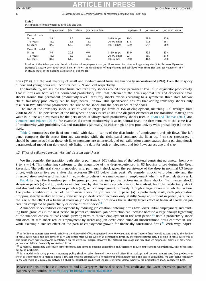
Table 2
Distribution of employment by firm size and age.
Employment Job creation Job destruction Employment Job creation Job destruction
Panel A: data
Births 2.8 18.5 0.0 1–19 emps 19.3 28.0 23.0
1–5 years 13.2 16.5 15.7 20–99 emps 17.8 17.5 18.1
6 + years 84.0 65.0 84.3 100 + emps 62.9 54.4 58.9
Panel B: model
Births 3.0 20.3 0.0 1–19 emps 18.9 33.8 23.4
1–5 years 13.1 15.2 16.5 20–99 emps 22.1 19.7 21.6
6 + years 84.0 64.5 83.5 100 + emps 59.0 46.5 55.0
Panel A of the table presents the distribution of employment and job flows over firm size and age categories % in Business Dynamics
Statistics database over 20 0 0–20 06. Panel B shows the distribution of employment and job flows over firms size and age categories in %
in steady state of the baseline calibration of our model.
firms (91%), but the vast majority of small and medium-sized firms are financially unconstrained (89%). Even the majority
of new and young firms are unconstrained: 70% and 77% respectively.
For tractability, we assume that firms face transitory shocks around their permanent level of idiosyncratic productivity.
That is, firms are born with a permanent productivity level that determines the firm’s optimal size and experience small
shocks around this permanent productivity level. Transitory shocks evolve according to a symmetric three state Markov
chain: transitory productivity can be high, neutral, or low. This specification ensures that adding transitory shocks only
results in two additional parameters: the size of the shock and the persistence of the shock.
The size of the transitory shock is set at 2.5% to target job flows of 15% of employment, matching BDS averages from
20 0 0 to 20 06. The persistence of the idiosyncratic shock is set at 0.6 (the diagonal elements of the transition matrix); this
value is in line with estimates for the persistence of idiosyncratic productivity shocks used in Khan and Thomas (2013) and
Clementi and Palazzo (2016) . For example, if current productivity is at its neutral level, the firm remains at the same level
of productivity with probability 0.6 and transitions (annually) to either high or low productivity with probability 0.2 respec-
tively.
Table 2 summarizes the fit of our model with data in terms of the distribution of employment and job flows. The left
panel compares the fit across firm age categories while the right panel compares the fit across firm size categories. It
should be emphasized that these job flows moments are untargeted, and our calibration demonstrates that a parsimoniously
parameterized model can do a good job fitting the data for both employment and job flows across age and size.
4.2. Effect of collateral, productivity and discount rate shocks
We first consider the transition path after a permanent 20% tightening of the collateral constraint parameter from χ =8 to χ = 6 . 4 . This tightening conforms to the magnitude of the drop experienced in US housing prices during the Great
Recession. The collateral shock is modeled as a permanent shock given the persistence of the drop in nominal US house
prices, with prices five years after the recession 20–25% below their peak. We consider shocks to productivity and the
intermediation wedge ω of sufficient magnitude to deliver the same decline in employment when the Frisch elasticity is 1.
Fig. 4 displays the transition paths for gross job creation and job destruction under these shocks. The financial shock,
shown in panels (a) and (b), reduces employment by sharply reducing job creation. In contrast, both the productivity shock
and discount rate shock, shown in panels (c)–(f), reduce employment primarily through a large increase in job destruction.
The partial equilibrium effect of the financial shock on job creation in panel (a) is particularly stark, with job creation
dropping sharply relative to steady state while job destruction increases only slightly. Wage adjustment in panel (b) reduces
the size of the effect of a financial shock on job creation but preserves the relatively larger effect of financial shocks on job
creation compared to productivity or discount rate shocks. 24
A financial shock reduces employment by reducing job creation; entering firms have lower initial employment and exist-
ing firms grow less in the next period. In partial equilibrium, job destruction can increase because a large enough tightening
of the financial constraint leads some growing firms to reduce employment in the next period. 25 Both a productivity shock
and discount rate shock reduce employment by increasing job destruction since all unconstrained firms contract in size,
while exerting a smaller effect on the path of employment growth for financially constrained firms. 26 With wage adjust-
24 A decline in interest rates would reinforce the differential effect em phasized here. Unconstrained firms (mature firms) would expand due to the decline
in rental rates, while the gap between MPK and rental rates would worsen at constrained firms. By increasing optimal size, a decline in rental rates would
also cause more firms to become constrained on the extensive margin. However, the patterns across age and size that we emphasize below are preserved—
job creation falls at financially constrained firms. 25 A financial shock may also cause some unconstrained firms to become constrained and, therefore, reduce employment. Quantitatively, this effect turns
out to be negligible. 26 In a model with sticky prices, a monetary policy shock or other demand shock would affect firm markups and the real interest rate. Our productivity
shock is isomorphic to a markup shock if retailers costless differentiate a homogenous intermediate good and sell to consumers. We also derive explicitly
in the appendix an equivalence between a shock to household credit that induces consumer deleveraging to the productivity shock considered here.
Please cite this article as: N. Mehrotra and D. Sergeyev, Financial shocks, firm credit and the Great Recession, Journal of
Monetary Economics, https://doi.org/10.1016/j.jmoneco.2020.01.008

N. Mehrotra and D. Sergeyev / Journal of Monetary Economics xxx (xxxx) xxx 11
ARTICLE IN PRESS
JID: MONEC [m3Gsc; February 12, 2020;3:33 ]
0 105years
-0.4
-0.2
0
0.2
% c
hang
e re
lativ
e to
SS
(a) Financial Shock (Frisch= )
Job DestructionJob Creation
0 105years
-0.04
-0.02
0
0.02
0.04
0.06
% c
hang
e re
lativ
e to
SS
(b) Financial Shock (Frisch=1)
Job DestructionJob Creation
0 105years
-0.4
-0.2
0
0.2
% c
hang
e re
lativ
e to
SS
(c) Productivity Shock (Frisch= )
Job DestructionJob Creation
0 105years
-0.04
-0.02
0
0.02
0.04
0.06
% c
hang
e re
lativ
e to
SS
(d) Productivity Shock (Frisch=1)
Job DestructionJob Creation
0 105years
-0.4
-0.2
0
0.2
% c
hang
e re
lativ
e to
SS
(e) Discount Rate Shock (Frisch= )
Job DestructionJob Creation
0 105years
-0.04
-0.02
0
0.02
0.04
0.06
% c
hang
e re
lativ
e to
SS
(f) Discount Rate Shock (Frisch=1)
Job DestructionJob Creation
Fig. 4. Job flows impulse responses. The figure displays the transition paths for gross job creation and job destruction after the financial, productivity, and
discount rate shocks. The numbers plotted display changes relative to the initial (steady state) levels. For example, job creation declines by 45% on impact
after the financial shock in case of infinite Frisch elasticity. The effects of the financial shock are shown in panels (a) and (b), the productivity shock effects
are shown in panels (c) and (d), and the discount rate shock effects in panels (e) and (f).
ment, job creation rises after a discount rate shock because the fall in the real wage dominates the effect of more costly
capital on asset accumulation for financially constrained, growing firms.
The differential behavior of job flows in response to financial shocks and the other two shocks fits the response of job
flows seen in the last two recessions as seen in Fig. 1 —the 2001 recession was characterized by a relatively sharp response
of job destruction, while the 2008 recession was characterized by a strong response of job creation. 27 Indeed, in 2008, job
destruction did not exceed the levels reached in a much milder recession in 2001. These findings are also consistent with
Foster et al. (2014) who use state level data to observe that total reallocation (sum of job creation and job destruction) fell
in the Great Recession in contrast to the three other recessions since 1980. As Fig. 4 illustrates, TFP and discount rate shocks
raise total reallocation while financial shocks cause a decline.
Age and size effects. Table 3 displays the effect of the shocks on the distribution of job creation and job destruction by
age and size categories. The table shows the average effect over the first three years after a shock with job flows expressed
as percentage changes from their initial level. The left-hand column displays the job flows effects of a financial shock, the
middle columns show the effect of a productivity shock, and the right hand columns show the effect of a discount rate
27 Job destruction rates (as opposed to levels) do increase more sharply after a financial shock.
Please cite this article as: N. Mehrotra and D. Sergeyev, Financial shocks, firm credit and the Great Recession, Journal of
Monetary Economics, https://doi.org/10.1016/j.jmoneco.2020.01.008

12 N. Mehrotra and D. Sergeyev / Journal of Monetary Economics xxx (xxxx) xxx
ARTICLE IN PRESS
JID: MONEC [m3Gsc; February 12, 2020;3:33 ]
Table 3
Effect of shocks on job flows.
Frisch elasticity Financial shock Productivity shock Productivity shock
α 0 1 α 0 1 α 0 1
Panel A: Job creation
Aggregate −0.24 −0.04 −0.05 −0.15 0.00 −0.01 −0.14 0.02 0.01
Age Births −0.12 −0.07 −0.07 −0.07 0.00 0.00 −0.06 0.01 0.01
1–5 years −0.47 −0.31 −0.32 −0.12 0.01 0.00 −0.09 0.05 0.04
6 + years −0.23 0.02 0.00 −0.18 0.00 −0.01 −0.18 0.01 0.00
Size 1–19 emps −0.07 0.05 0.04 −0.06 −0.01 −0.01 −0.07 0.00 −0.01
20–99 emps −0.33 −0.11 −0.12 −0.17 0.02 0.00 −0.15 0.04 0.02
100 + emps −0.35 −0.08 −0.10 −0.21 0.01 −0.01 −0.19 0.02 0.01
Panel B: Job destruction
Aggregate −0.04 −0.04 −0.04 0.06 0.00 0.01 0.08 0.02 0.03
Age 1–5 years −0.07 −0.06 −0.07 0.02 0.00 0.01 0.03 0.00 0.02
6 + years −0.04 −0.03 −0.03 0.07 −0.01 0.01 0.08 −0.03 0.03
Size 1-19emps 0.00 0.02 0.02 0.07 −0.01 0.01 0.07 −0.04 0.01
20–99 emps −0.07 −0.07 −0.07 0.06 0.00 0.01 0.07 −0.01 0.03
100 + emps −0.05 −0.05 −0.05 0.07 −0.01 0.01 0.08 −0.02 0.03
The table displays the effect of permanent negative financial shock (a 20% decline in collateral constraint parameter), permanent negative
productivity shocks (the size of the shock produces the same long-run decline in aggregate employment level as 20% financial shock), and
permanent increase in discount rate wedge (the size of the shock produces the same long-run decline in aggregate employment level as
20% financial shock) on the distribution of job creation and job destruction by firm age and size categories. The table shows the average
effect over the first three years after the shock with job flows expressed as changes relative to the initial (steady state) level. For example,
aggregate job creation declines by 24% on average over the first three years after the shock. The first three columns display the job flows
effects of a permanent financial shock, the next three columns display the job flows effects of a permanent productivity shock, the last
three columns show the effects of the wedge shock. Each column conforms to different values for the Frisch elasticity: an infinite Frisch
elasticity (rigid wages), zero Frisch elasticity (vertical labor supply), and the last column is our preferred specification.
shock. For each shock, we show how these responses depend on the Frisch elasticity: first column is the case of an infinite
Frisch elasticity (rigid wages), the second column is the case of a zero Frisch elasticity (vertical labor supply), and the last
column is our baseline specification.
The effect of a collateral shock on job creation is strongest at young firms followed by new firms, with mature firms
exhibiting the weakest response (as long as wages adjust). The job creation response is relatively stronger at young firms
as opposed to new firms due to the absence of any extensive margin response. An endogenous entry decision would likely
amplify the fall in job creation at new firms. General equilibrium effects are crucial for the finding that job creation at new
and young firms falls more than mature firms. In partial equilibrium, the financial shock has a large effect on job creation at
mature firms since the highest productivity firms remain financially constrained even after 5 years. However, when wages
adjust, the unconstrained mature firms create jobs offsetting the decline in job creation at financially constrained, mature
firms. In contrast, productivity shocks have more uniform effects on job creation across ages, while discount rate shocks
disproportionately impact mature firms. With wage adjustment, job creation turns positive in all age categories as lower
wages cause constrained firms to create more jobs. The difference in the age effect on job creation is a key difference
between productivity and discount rate shocks.
Across firm size categories, our model predicts that financial shocks will have the largest effect on job creation at
medium-size firms (20–99 employees) followed by large firms (100+ employees) and small firms (1–19 employees). This
perhaps counterintuitive result stems from the fact that the collateral constraint is most important for firms with relatively
higher productivity levels. Low productivity firms are largely unaffected by a tightening of constraints. When wages fall,
small firms create jobs since their optimal size rises with lower wages. Relatively high productivity firms that start small
transit through the medium-sized category; effectively, this size category is the best proxy for financially constrained firms.
Job creation falls less at large firms because unconstrained large firms create jobs that offset the decline in job creation
at the large constrained firms. Both productivity and discount rate shocks have their largest effect on job creation at large
firms; with GE effects, however, differences in job creation across size are less uniform for discount rate shocks versus
productivity shocks. Moreover, the GE effect of falling wages is sufficiently strong after a discount rate shock to raise job
creation across more size categories.
Our model predicts that job destruction after a financial shock falls at both young and mature firms with a relatively
larger response at young firms. On impact, job destruction rises at both young and mature firms since tighter financial
constraints lower capital and labor demand. After impact, destruction falls at young firms because they become smaller after
the collateral shock. Therefore, the jobs destroyed by these firms when they exit also fall. By contrast, for mature firms, there
are two competing effects after impact: given exogenous exit rates, fewer firms survive to their optimal size reducing job
destruction; however, as wages fall, optimal size increases for unconstrained firms leading to greater job destruction when
these firms exit. The job destruction patterns for a financial shock by firm age largely mirror the job creation patterns. Job
destruction falls at medium sized firms; these firms are smaller after the financial shock and destroy fewer jobs during exit.
By contrast, productivity and discount rate shocks generate much more uniform effects across firm size with both the sign
Please cite this article as: N. Mehrotra and D. Sergeyev, Financial shocks, firm credit and the Great Recession, Journal of
Monetary Economics, https://doi.org/10.1016/j.jmoneco.2020.01.008

N. Mehrotra and D. Sergeyev / Journal of Monetary Economics xxx (xxxx) xxx 13
ARTICLE IN PRESS
JID: MONEC [m3Gsc; February 12, 2020;3:33 ]
0 105years
-0.3
-0.25
-0.2
-0.15
-0.1
-0.05
0%
cha
nge
rela
tive
to S
S
Job Creation
ModelData (2008-2012)
0 105years
-0.3
-0.2
-0.1
0
0.1
0.2
% c
hang
e re
lativ
e to
SS
Job Destruction
ModelData (2008-2012)
Fig. 5. Job flows paths in the model and in the data. The figure displays the paths for gross job creation and job destruction after the shocks that occur in
period 1 in the model and in the data. The numbers plotted display changes relative to the initial (steady state) levels. The four shocks that drive model
dynamics are chosen to match the initial changes (between 2008 and 2009) in job flows in the data.
and ordering contrasting with a financial shock. Like the job creation patterns, a discount rate shock has somewhat less
uniform job destruction effects across age and size than productivity shocks.
4.3. Shocks decomposition
Given that financial, productivity, and discount rate shocks impact employment via distinct margins and have heteroge-
nous effects across firm age, we can use job flows to decompose the contribution of these factors to the decline in employ-
ment experienced in the US during the Great Recession. As seen in Fig. 4 , financial vs. productivity/discount rate shocks that
lead to the same long-run decline in employment have dramatically different effects on aggregate job flows. This differen-
tial behavior along with the differences in the effect of all three shocks across firm age allow us to determine their relative
contributions.
In addition to the financial shock, a shock to initial assets a 0 is also considered; like a shock to the leverage ratio χ , this
shock also impairs the ability of new and young firms to hire workers. On its own, a shock to a 0 is qualitatively similar to
the a shock to χ . In our estimation, the joint effect of shocks to χ and a 0 is labeled as the financial (or firm credit) shock.
A shock to a 0 is an admittedly abbreviated way to incorporate the effects of a financial shock on firm entry and we have
experimented with shock decompositions holding a 0 constant. 28
We nonlinearly estimate a financial, productivity, discount rate, and initial asset shock on a grid to best match initial
changes in aggregate job flows and job flows across firm age categories in the Great Recession in the US. 29 It is clear from
Fig. 1 that a sharp decline in aggregate job creation and sharp increase in job destruction occurred between 2007Q4 and
2009Q1. In the annualized data coming from the BDS, similar magnitudes of changes in job flows are observed between
March 2008 and March 2009. We focus on the initial difference between these two years because only annual data for the
job flows is available by firm categories.
To match the initial changes in job flows we estimate a productivity shock of -1.3%, a financial ( χ ) shock of −20.8%, a
discount rate shock of ω = 0 . 01 , and an initial asset ( a 0 ) shock of −23%. 30 Fig. 5 compares the behavior of aggregate job
28 In a microfounded model of entry, the entry decision depends on a comparison of the value of operating a business relative to the outside option.
Moreover, what matters for the estimation is the differential sensitivity of these values to the structural shocks. In particular, a financial shock may exert
a positive selection effect where high productivity entrepreneurs choose to enter mitigating the effect on job creation. 29 Formally, the following objective is minimized by choosing the four shocks on a grid:
O = ( � log JC model −� log JC data ) 2 + ( � log JD model −� log JD data )
2 + �∑
i
μi
(� log JC i model − � log JC i data
)2 + �∑
j
μ j
(� log JD
j
model −� log JD
j
data
)2 ,
where i ∈ { new, young, mature } and j ∈ { young , mature }, μi is the number of people employed by firms belonging to category i in stationary equilibrium
relative to aggregate employment, � = 0 . 05 indexes the importance of matching category specific job flows relative to aggregate job flows. As a result, we
pick four shocks to best match seven moments. The small value of � ensures an accurate match of the on-impact behavior of aggregate job flows. 30 The financial shock by itself generates a decline in measured TFP of 0.4% due to increased misallocation.
Please cite this article as: N. Mehrotra and D. Sergeyev, Financial shocks, firm credit and the Great Recession, Journal of
Monetary Economics, https://doi.org/10.1016/j.jmoneco.2020.01.008

14 N. Mehrotra and D. Sergeyev / Journal of Monetary Economics xxx (xxxx) xxx
ARTICLE IN PRESS
JID: MONEC [m3Gsc; February 12, 2020;3:33 ]
0 5 10-0.4
-0.2
0
chan
ge fr
om S
S Employment (births)
0 5 10-0.4
-0.2
0Employment (young)
0 5 10-0.1
0
0.1Employment (mature)
0 105years
-0.2
-0.1
0
chan
ge fr
om S
S JC (births)
0 5 10-0.4
-0.2
0JC (young)
0 5 10-0.5
0
0.5JC (mature)
ModelData (2008-2012)
0 105years
-0.5
0
0.5
chan
ge fr
om S
S JD (young)
0 105years
-0.2
0
0.2JD (mature)
Fig. 6. Job flows paths in the model and in the data across firm age categories. The figure displays the paths for gross job creation and job destruction
after the shocks that occur in period 1 in the model and in the data across new, young and mature firms. The numbers plotted display changes relative to
the initial (steady state) levels. For example, the on impact decline in job creation at new firms is 20%.
flows in the model and the data. Job flows in the model match the behavior of job flows in the data on impact. Our model
captures the initial dynamics of aggregate job flows but underestimates more recent job creation given the assumption of
a permanent shock. US job creation recovers somewhat by 2012 as financial conditions have normalized and employment
growth accelerated.
Fig. 6 compares employment and job flows in our model across different firm age categories to their data counterparts.
Our model matches the behavior of employment and job flows fairly well. Our model slightly overpredicts the fall on impact
in job creation at young firms, but this discrepancy may be related to the particularly stark nature of the financial shock
that impacts all young firms at the same time instead of more slowly impacting these firms over time as they seek to secure
fresh financing for expansion. The initial asset shock also does well in matching the fall in job creation and employment at
new firms. 31
Fig. 7 shows the model predictions about employment and job flows dynamics across firm size categories. The model
matches the data for employment and job flows dynamics for medium and large firms fairly well. These movements in
employment and job flows by size are not targeted by our estimation strategy; these overidentified moments provide addi-
tional confidence in our shock decomposition. Finally, our model also generates a decline in the ratio of external borrowing
to the capital stock of 10% on impact—in line with the decline in borrowing documented by Buera et al. (2015) .
Finally, because we use shocks in the model to match the initial changes in the job flows in the recent US recession, we
can study the relative importance of these shocks for explaining the employment decline. The ratio of the long-run decline
in employment driven only by the shock to χ and a 0 to the decline driven by all four shocks is 0.18; the same ratio for
the productivity shock is 0.26 and for the discount rate shock is 0.58. 32 Our decomposition indicates that, despite being
fairly large, the overall disruption to firm credit can explain only about 18% of the decline in employment in the Great
Recession. 33 The equivalent decomposition estimating three shocks and holding a 0 constant finds that 15% of the decline
in employment is explained by just the χ shock alone. Significant aggregate shocks including the discount rate shock are
31 If we hold a 0 constant, a three shock decomposition shows that the χ shock only captures about half the decline in job creation at new firms in the
Great Recession. 32 Observe that the three numbers may not sum up to one because of the nonlinear interaction effects. Also note that the on-impact break-down of the
effects of the shocks are 11% ( χ and a 0 ), 27% (productivity), 63% (discount rate). The initial impact of financial shocks χ and a 0 increases over time because
the distribution of firms across size shifts to the left. We focus on the long-run effect because it gives us an upper bound on the effect of χ and a 0 shocks. 33 In this respect, our findings are closer to the findings of Mian and Sufi (2014) or Greenstone et al. (2014) who argue that the credit supply channel
explains a relatively small part of the decline in US employment.
Please cite this article as: N. Mehrotra and D. Sergeyev, Financial shocks, firm credit and the Great Recession, Journal of
Monetary Economics, https://doi.org/10.1016/j.jmoneco.2020.01.008

N. Mehrotra and D. Sergeyev / Journal of Monetary Economics xxx (xxxx) xxx 15
ARTICLE IN PRESS
JID: MONEC [m3Gsc; February 12, 2020;3:33 ]
0 5 10-0.1
0
0.1
chan
ge fr
om S
S
Employment (small)
0 5 10-0.2
-0.1
0Employment (medium)
0 5 10-0.1
0
0.1Employment (large)
0 5 10-0.2
-0.1
0
chan
ge fr
om S
S
JC (small)
0 5 10-0.5
0
0.5JC (medium)
0 5 10-0.4
-0.2
0JC (large)
0 105years
-0.5
0
0.5
chan
ge fr
om S
S
JD (small)
0 105years
-0.5
0
0.5JD (medium)
0 105years
-0.5
0
0.5JD (large)
Fig. 7. Job flows paths in the model and in the data across firm size categories. The figure displays the paths for gross job creation and job destruction
after the shocks that occur in period 1 in the model (blue solid lines) and in the data (orange lines with dot markers) across small, medium and large
firms. The numbers plotted display changes relative to the initial (steady state) levels. For example, the on impact decline in job creation at small firms is
about 19%. (For interpretation of the references to color in this figure legend, the reader is referred to the web version of this article.)
needed to explain the overall decline in employment. 34 The productivity and discount rate shock used here may themselves
be driven by financial factors (productivity may proxy for declines in demand due to consumer deleveraging or the discount
rate shock may proxy for a flight to safety), but our estimation concludes that these shocks that broadly impact all firms
are needed for explaining the overall decline in US employment. 35
5. Empirical strategy and results
Our model delivers testable implications for effects of a financial shock on job flows. We can validate our model and
build confidence in the shock decomposition by examining whether these relationships hold in cross-city data on US job
flows.
5.1. Empirical strategy
Any test of the hypothesis that an increase in financial frictions diminishes job flows must overcome several challenges
of both measurement and causality. Our empirical strategy addresses these issues by using MSA-level variation in job flows
and financial conditions to determine the causal effect of firm credit shocks on job flows.
The first issue to confront is finding suitable proxy for financial conditions at the MSA level. Given the lack of detailed
data on firm balance sheets, we use data on the growth rate of MSA house prices as a proxy for financing conditions.
House prices are an appropriate proxy for firm financing conditions for two reasons. First, movements in housing prices
can directly affect the financing capacity of firms by impacting the net worth of entrepreneurs. 36 Second, falling house
prices may impair the ability of younger and medium-sized firms to post collateral for bank loans. Recent empirical work
34 The limited contribution of the financial shock to the decline in employment is due in large measure to general equilibrium effects. The decrease in
employment at financially constrained firms is offset by an increase in employment at financially unconstrained firms since wages fall and their optimal
size grows. This same offsetting effect does not occur with a productivity shock. 35 Our estimation is largely unchanged when we seek to match job flow rates (as opposed to levels); the importance of the discount rate shock is slightly
lessened with the estimation now increasing the role of the productivity shock. 36 Fairlie and Krashinsky (2012) provide direct evidence for changes in housing equity on entrepreneurship using data from the Current Population Survey,
while Schmalz et al. (2013) show in French data that higher house prices increase the probability of becoming an entrepreneur and, conditional on starting
a business, increase the initial scale of the firm. Adelino et al. (2013) also document the importance of the collateral channel in the employment at small
establishments.
Please cite this article as: N. Mehrotra and D. Sergeyev, Financial shocks, firm credit and the Great Recession, Journal of
Monetary Economics, https://doi.org/10.1016/j.jmoneco.2020.01.008

16 N. Mehrotra and D. Sergeyev / Journal of Monetary Economics xxx (xxxx) xxx
ARTICLE IN PRESS
JID: MONEC [m3Gsc; February 12, 2020;3:33 ]
by Chaney et al. (2012) shows that fluctuations in local house prices even affect larger public companies in Compustat by
reducing collateral values. 37 Lastly, changes in housing prices can affect the availability of local bank credit to firms via
losses/defaults on a bank’s mortgage portfolio. These losses, whether via the household or commercial loan portfolio, raise
the cost of bank credit.
In addition to finding a suitable proxy for financial frictions, the relative dearth of job flows data in the time series limits
any analysis of the effect of financial frictions on job flows in the aggregate data. Instead, we exploit MSA-level variation in
job flows and housing prices to improve the power of our estimates and increase useful variation from state and regional
housing booms.
The most significant challenge in establishing a causal effect of housing price movements on job flows is ruling out
an aggregate demand channel that drives a correlation between job flows and housing prices. We address this concern in
several ways. Firstly, location and time fixed effects are included to account for the business cycle and differences across
MSAs in job flows. Secondly, to control for MSA-specific demand shocks, controls are included for the local business cycle.
Our baseline regression takes the following form:
y it = αi + δt + γ ( L ) �GSP it + β( L ) �hp it + εit ,
where y it is job creation or job destruction for MSA i at time t . �GSP it represents the growth rate of the MSA-level business
cycle variable, while �hp it is the growth rate of MSA housing prices. Our coefficient of interest is the sum of the coefficients
β(1) on MSA housing prices. A positive coefficient indicates that falling house prices decrease job flows over a three-year
period (to facilitate comparison with the model responses).
Alternatively, we also consider two IV strategies following the methodology laid out in the empirical literature on the
effects of housing price shocks. Under the first approach, which we call “the dummy approach,” MSA-level house price
growth is instrumented with US house price growth interacted with an MSA dummy. This IV strategy is similar to the
methodology used in Nakamura and Steinsson (2014) in their study of government spending multipliers.
Our other IV strategy, which we call “the Saiz approach,” interacts the MSA-level land supply elasticities computed in
Saiz (2010) with national house prices. In both cases, the identifying assumption is that whatever causes movements in
national house prices are uncorrelated with MSA-specific aggregate demand shocks. Our IV regression takes the following
form:
y it = αi + δt + β( L ) �˜ hp it + εit (2nd stage)
�hp it = αi + δt + ρi (L )�hp t + u it (1st stage)
where �˜ hp it is the fitted value for MSA house prices obtained from the first-stage regression of MSA house prices on
national house prices interacted with an MSA dummy or with the Saiz land supply elasticity. As before, the coefficient of
interest is the sum of coefficients β(1) measuring the effect of housing prices on job flows.
We further decompose the effect of housing prices on job flows by firm size and firm age categories, utilizing both OLS
and IV specifications. In addition to MSA and time fixed effects, category fixed effects are included. In these regressions, both
the MSA business cycle variable and MSA house prices are allowed to have differential effects on job flows across categories,
and our coefficient of interest is the sum of coefficients of MSA house prices by category. The IV specification is analogous
to the IV specification for aggregate job flows, where the instrument is now national house price growth interacted with a
MSA-category dummy or the MSA land supply elasticity.
Importantly, it is worth stressing that our empirical strategy cannot rule out effects on job flows through the home-
equity channel emphasized by Mian and Sufi (2014) . Even if our IV approach successfully identifies exogenous housing price
shocks, the effect of these shocks on job creation and job destruction may be driven by a decline in consumer demand due
to a decline in household wealth. However, in the Appendix E, we compare the behavior of employment at new firms versus
employment at new establishments of existing firms; we argue that the fact that new establishments of existing firms do
not respond to house price shocks (after controlling for local business cycles) provides evidence in favor of the credit supply
channel. The patterns documented are also shown to hold within tradeable and non-tradeable industry classifications and
after excluding construction.
5.2. Data
Several distinct data sources are used for measures of job flows, house prices, and MSA measures of the business cycle.
Data on job flows comes from the Business Dynamics Statistics (BDS), which is drawn from the Census Bureau’s Longitudinal
Database (LBD), a confidential database that tracks employment at the establishment and firm level over time. Specifically,
data on gross job creation and job destruction at the MSA level from 1982 to 2012 are used for 366 MSAs resulting in a
panel of 31 x 366 observations.
House price data comes from the Federal Housing Finance Agency’s MSA house price indices. The all-transactions indexes
which provide a quarterly time series of housing prices from 1975 to present are utilized. MSA-level business cycle measures
37 One may be concerned that residential real estate prices are a poor proxy for commercial real estate. These authors use residential real estate prices
and show that their results hold in a subset of their data for which commercial real estate prices are available.
Please cite this article as: N. Mehrotra and D. Sergeyev, Financial shocks, firm credit and the Great Recession, Journal of
Monetary Economics, https://doi.org/10.1016/j.jmoneco.2020.01.008
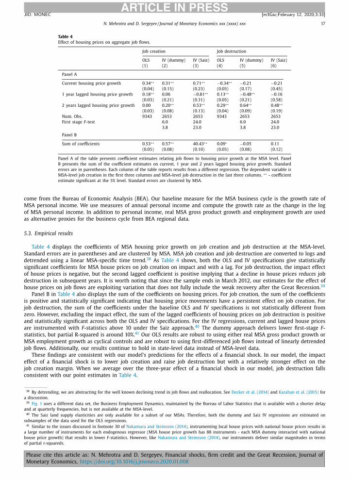
N. Mehrotra and D. Sergeyev / Journal of Monetary Economics xxx (xxxx) xxx 17
ARTICLE IN PRESS
JID: MONEC [m3Gsc; February 12, 2020;3:33 ]
Table 4
Effect of housing prices on aggregate job flows.
Job creation Job destruction
OLS IV (dummy) IV (Saiz) OLS IV (dummy) IV (Saiz)
(1) (2) (3) (4) (5) (6)
Panel A
Current housing price growth 0.34 ∗∗ 0.31 ∗∗ 0.71 ∗∗ −0.34 ∗∗ −0.21 −0.21
(0.04) (0.15) (0.23) (0.05) (0.17) (0.45)
1 year lagged housing price growth 0.18 ∗∗ 0.06 −0.81 ∗∗ 0.13 ∗∗ −0.48 ∗∗ −0.16
(0.03) (0.21) (0.31) (0.05) (0.21) (0.58)
2 years lagged housing price growth 0.00 0.20 ∗∗ 0.53 ∗∗ 0.29 ∗∗ 0.64 ∗∗ 0.48 ∗∗
(0.03) (0.08) (0.13) (0.04) (0.09) (0.19)
Num. Obs. 9343 2653 2653 9343 2653 2653
First stage F -test 6.0 24.0 6.0 24.0
3.8 23.0 3.8 23.0
Panel B
Sum of coefficients 0.53 ∗∗ 0.57 ∗∗ 40.43 ∗∗ 0.09 ∗ −0.05 0.11
(0.05) (0.08) (0.10) (0.05) (0.08) (0.12)
Panel A of the table presents coefficient estimates relating job flows to housing price growth at the MSA level. Panel
B presents the sum of the coefficient estimates on current, 1 year and 2 years lagged housing price growth. Standard
errors are in parentheses. Each column of the table reports results from a different regression. The dependent variable is
MSA-level job creation in the first three columns and MSA-level job destruction in the last three columns. ∗∗ - coefficient
estimate significant at the 5% level. Standard errors are clustered by MSA.
come from the Bureau of Economic Analysis (BEA). Our baseline measure for the MSA business cycle is the growth rate of
MSA personal income. We use measures of annual personal income and compute the growth rate as the change in the log
of MSA personal income. In addition to personal income, real MSA gross product growth and employment growth are used
as alternative proxies for the business cycle from BEA regional data.
5.3. Empirical results
Table 4 displays the coefficients of MSA housing price growth on job creation and job destruction at the MSA-level.
Standard errors are in parentheses and are clustered by MSA. MSA job creation and job destruction are converted to logs and
detrended using a linear MSA-specific time trend. 38 As Table 4 shows, both the OLS and IV specifications give statistically
significant coefficients for MSA house prices on job creation on impact and with a lag. For job destruction, the impact effect
of house prices is negative, but the second lagged coefficient is positive implying that a decline in house prices reduces job
destruction in subsequent years. It is worth noting that since the sample ends in March 2012, our estimates for the effect of
house prices on job flows are exploiting variation that does not fully include the weak recovery after the Great Recession. 39
Panel B in Table 4 also displays the sum of the coefficients on housing prices. For job creation, the sum of the coefficients
is positive and statistically significant indicating that housing price movements have a persistent effect on job creation. For
job destruction, the sum of the coefficients under the baseline OLS and IV specifications is not statistically different from
zero. However, excluding the impact effect, the sum of the lagged coefficients of housing prices on job destruction is positive
and statistically significant across both the OLS and IV specifications. For the IV regressions, current and lagged house prices
are instrumented with F -statistics above 10 under the Saiz approach. 40 The dummy approach delivers lower first-stage F -
statistics, but partial R-squared is around 10%. 41 Our OLS results are robust to using either real MSA gross product growth or
MSA employment growth as cyclical controls and are robust to using first-differenced job flows instead of linearly detrended
job flows. Additionally, our results continue to hold in state-level data instead of MSA-level data.
These findings are consistent with our model’s predictions for the effects of a financial shock. In our model, the impact
effect of a financial shock is to lower job creation and raise job destruction but with a relatively stronger effect on the
job creation margin. When we average over the three-year effect of a financial shock in our model, job destruction falls
consistent with our point estimates in Table 4 .
38 By detrending, we are abstracting for the well known declining trend in job flows and reallocation. See Decker et al. (2014) and Karahan et al. (2015) for
a discussion. 39 Fig. 1 uses a different data set, the Business Employment Dynamics, maintained by the Bureau of Labor Statistics that is available with a shorter delay
and at quarterly frequencies, but is not available at the MSA-level. 40 The Saiz land supply elasticities are only available for a subset of our MSAs. Therefore, both the dummy and Saiz IV regressions are estimated on
subsamples of the data used for the OLS regressions. 41 Similar to the issues discussed in footnote 30 of Nakamura and Steinsson (2014) , instrumenting local house prices with national house prices results in
a large number of instruments for each endogenous regressor (MSA house price growth has 88 instruments - each MSA dummy interacted with national
house price growth) that results in lower F -statistics. However, like Nakamura and Steinsson (2014) , our instruments deliver similar magnitudes in terms
of partial r-squareds.
Please cite this article as: N. Mehrotra and D. Sergeyev, Financial shocks, firm credit and the Great Recession, Journal of
Monetary Economics, https://doi.org/10.1016/j.jmoneco.2020.01.008

18 N. Mehrotra and D. Sergeyev / Journal of Monetary Economics xxx (xxxx) xxx
ARTICLE IN PRESS
JID: MONEC [m3Gsc; February 12, 2020;3:33 ]
Table 5
Effect of housing prices on job flow by firm age.
Job creation Job destruction
OLS IV (dummy) IV (Saiz) OLS IV (dummy) IV (Saiz)
(1) (2) (3) (4) (5) (6)
Panel A
Births 0.88 ∗∗ 0.66 ∗∗ 0.68 ∗∗
(0.07) (0.09) (0.13)
Young Firms, 0.48 ∗∗ 0.63 ∗∗ 0.55 ∗∗ 0.36 ∗∗ 0.20 ∗∗ 0.47 ∗∗
1–5 years (0.07) (0.11) (0.14) (0.07) (0.09) (0.13)
Mature Firms, 0.33 ∗∗ 0.31 ∗∗ −0.01 −0.06 −0.19 ∗∗ −0.03
6 + years (0.05) (0.09) (0.15) (0.06) (0.08) (0.12)
Num. Obs. 28,029 7959 7959 18,686 5306 5306
Panel B
H = Births - Mature 0.55 ∗∗ 0.36 ∗∗ 0.69 ∗∗ 0.43 ∗∗ 0.40 ∗∗ 0.50 ∗∗
or Young - Mature (0.08) (0.08) (0.14) (0.07) (0.07) (0.13)
The table presents the effect of housing price growth at the MSA level on job flows by firm age cate-
gories (births, 1–5 and 6+ years old). Each column in the table reports results from a different regres-
sion. The dependent variable is job creation in the first three columns and job destruction in the last
three columns. The numbers reported are the sum of the effects of current, 1 year and 2 years lagged
changes in house price growth on job flows by firms age. Standard errors are in parentheses. The first
three columns of panel B reports the difference in the effect of housing price changes on job flows
between new and mature firms. The last three columns of panel B present the difference in the effect
of housing price between young and mature firms. ∗∗ - coefficient estimate significant at the 5% level, ∗- coefficient estimate significant at the 10% level. Standard errors are clustered by MSA.
We now turn to job flows responses by firm age categories: new firms, young firms (1–5 years of age), and mature firms
(6+ years of age). Table 5 shows the sum of coefficients on MSA housing prices, βh (1) under the OLS and IV specifications.
The table shows that job creation at new firms exhibit the strongest response to housing prices followed by job creation
at young firms. Job creation at mature firms exhibits the least sensitivity to house prices and, in the case of column (3),
is not statistically different from zero. Our model predicts that job creation should fall for new and young firms, and that
young firms should fall relatively more than mature firms. These predictions are verified in Panels A and B respectively of
Table 5 . 42
Job destruction at young firms shows a positive and statistically significant coefficient on housing prices, while job de-
struction at mature firms moves inversely to housing prices (though statistically significantly negative only in column (5)).
The last row of Table 5 shows that the difference in the sensitivity of job destruction to house prices between young firms
and mature firms is statistically significant under all specifications. The fall in job destruction at young firms and differential
effect on job destruction between young and mature firms is in line with our model predictions. 43
In addition to age, we examine job flows by firm size, and consider three categories. 44 Table 6 displays the results from
the firm size job flows regressions. For job creation, middle and large sized firms exhibit the highest sensitivity to housing
prices, followed by small firms consistent with our model predictions. In the case of the IV specification, the coefficient of
housing prices on job creation for small firms is negative meaning a decrease in house price growth raises job creation at
small firms. Our model predicts this behavior for job creation at small firms due the effect of falling wages that induces
unconstrained firms to expand.
Job destruction for middle-sized firms display a positive coefficient on housing prices under all specifications also in line
with our model, though the coefficients are not statistically significant under IV specifications. However, our model does
miss on job destruction for large firms - our model predicts a positive coefficient but lower than the coefficient for medium-
sized firms. However, the large positive coefficient for large firms is influenced by a large positive impact coefficient. 45
Table 6 also shows that the difference in coefficients between middle-sized firms and small firms is statistically significant
across all specifications for both job creation and job destruction. In contrast, the difference for middle and large sized firms
for job creation is generally not significant. Our model predicts the right signs and relative ordering for both creation and
destruction at small and middle-sized firms.
42 The first stage F -stats are not included in Tables 5 and 6 as they are the same as in Table 4 . 43 Fort et al. (2013) find that gross job destruction increases after a decline in house prices using state level data. The difference with our findings is
explained by their use of job destruction rates as opposed to detrended levels. 44 Firm size assigns size categories based on an average of employment in the previous year and employment in the current year raising potential issues
of reclassification bias (see Moscarini and Postel-Vinay (2012) for a discussion). However, initial firm size data is not available at the MSA level, and our
results are unchanged in state level data using size categories based on initial firm size. 45 If we restrict our attention to the lagged response, the empirical pattern across firm size categories is consistent with our model. Also, large firms are
more likely to operate across multiple MSAs somewhat complicating comparison of model and data for large firms. Our state level regressions (not shown)
find a coefficient of housing price shocks on job destruction at large firms that is lower than middle-sized firms consistent with model predictions.
Please cite this article as: N. Mehrotra and D. Sergeyev, Financial shocks, firm credit and the Great Recession, Journal of
Monetary Economics, https://doi.org/10.1016/j.jmoneco.2020.01.008

N. Mehrotra and D. Sergeyev / Journal of Monetary Economics xxx (xxxx) xxx 19
ARTICLE IN PRESS
JID: MONEC [m3Gsc; February 12, 2020;3:33 ]
Table 6
Effects on housing prices on job flows by firm size.
Job creation Job destruction
OLS IV (dummy) IV (Saiz) OLS IV (dummy) IV (Saiz)
(1) (2) (3) (4) (5) (6)
Panel A
1–19 employees 0.37 ∗∗ 0.25 ∗∗ −0.13 −0.10 ∗∗ −0.34 ∗∗ −0.43 ∗∗
(0.04) (0.06) (0.11) (0.04) (0.07) (0.11)
20–99 employees 0.75 ∗∗ 0.73 ∗∗ 0.66 ∗∗ 0.28 ∗∗ 0.01 0.18
(0.06) (0.06) (0.09) (0.06) (0.07) (0.11)
100 + employees 0.58 ∗∗ 0.81 ∗∗ 0.83 ∗∗ 0.13 ∗ 0.23 ∗∗ 0.56 ∗∗
(0.06) (0.09) (0.13) (0.08) 0.09 (0.12)
Num. Obs. 28,029 7959 7959 28,029 7959 7959
Panel B
H = (20–99 emp) 0.38 ∗∗ 0.49 ∗∗ 0.79 ∗∗ 0.38 ∗∗ 0.35 ∗∗ 0.60 ∗∗
- (1–19 emp) (0.04) (0.04) (0.09) (0.04) (0.05) (0.09)
The table presents the effect of housing price growth at the MSA level on job flows by firms size
categories (1-19, 20-99 and 100+ employees). Each column in the table reports results from a differ-
ent regression. The dependent variable is job creation in the first three columns and job destruction
in the last three columns. The numbers reported are the sum of the effects of current, 1 year and 2
years lagged changes in house price growth on job flows by firms size. Standard errors are in paren-
theses. Panel B reports the difference in the effect of housing price changes on job flows between
medium (20-99 employees) and small firms (1-19 employees). ∗∗ - coefficient estimate significant at
the 5% level. Standard errors are clustered by MSA.
6. Conclusion
The contribution of the firm credit channel to the decline in employment and job flows experienced in the Great Reces-
sion is analyzed in this paper. Using a simple model of firm dynamics in the presence of a collateral constraint, we show
how shocks to firm credit operate disproportionately on gross job creation margin and have stronger effects on job creation
at young firms and medium sized firms (20–99 employees). By contrast, shocks to productivity or shocks that raise risk
premia operate primarily on the job destruction margin and have more uniform effects across firm age and size.
Our benchmark model is calibrated to match US employment by firm size and age prior to the Great Recession. We
estimate the combination of shocks to firm credit, productivity, and risk premia that rationalize the response of overall
job flows and job flows by firm age. Our estimation finds that, despite its large magnitude, shocks to firm credit explain
only 18% of the decline in employment in the Great Recession. The productivity and risk premia shock are much more
important in quantitatively explaining the magnitude of the decline in employment. Lastly, we empirically validate the job
flows responses to financial shocks predicted by our model.
Supplementary material
Supplementary material associated with this article can be found, in the online version, at doi: 10.1016/j.jmoneco.2020.
01.008 .
References
Adelino, M. , Schoar, A. , Severino, F. , 2013. House Prices, Collateral and Self-Employment. Technical Report. National Bureau of Economic Research . Bacchetta, P. , Benhima, K. , Poilly, C. , 2019. Corporate cash and employment. Am. Econ. J.: Macroeconomics 11 (3), 30–66 .
Baker, S.R. , Bloom, N. , Davis, S.J. , 2016. Measuring economic policy uncertainty. Q. J. Econ. 131 (4), 1593–1636 . Beraja, M. , Hurst, E. , Ospina, J. , 2016. The Aggregate Implications of Regional Business Cycles. Technical Report. National Bureau of Economic Research .
Buera, F.J. , Fattal Jaef, R.N. , Shin, Y. , 2015. Anatomy of a credit crunch: from capital to labor markets. Rev. Econ. Dyn. 18 (1), 101–117 . Buera, F.J., Shin, Y., 2011. Self-insurance vs. self-financing: a welfare analysis of the persistence of shocks. J. Econ. Theory 146 (3), 845– 862. doi: 10.1016/j.
jet.2011.01.003 .
Caballero, R.J. , Farhi, E. , 2018. The safety trap. Rev. Econ. Stud. 85 (1), 223–274 . Chaney, T. , Sraer, D. , Thesmar, D. , 2012. The collateral channel: how real estate shocks affect corporate investment. Am. Econ. Rev. 102 (6), 2381–2409 .
Chari, V. , Christiano, L. , Kehoe, P. , 2013. The Behavior of Large and Small Firms Over the Business Cycle. Technical Report. Mimeo. University of Minnesota . Chodorow-Reich, G. , 2014. The employment effects of credit market disruptions: firm-level evidence from the 20 08–20 09 financial crisis. Quarterly Journal
of Economics 129 (1), 1–59 . Christiano, L.J. , Eichenbaum, M. , Evans, C.L. , 2005. Nominal rigidities and the dynamic effects of a shock to monetary policy. J. Political Econ. 113 (1), 1–45 .
Christiano, L.J. , Eichenbaum, M.S. , Trabandt, M. , 2015. Understanding the great recession. Am. Econ. J. 7 (1), 110–167 .
Clementi, G.L. , Palazzo, B. , 2016. Entry, exit, firm dynamics, and aggregate fluctuations. Am. Econ. J. 8 (3), 1–41 . Cooley, T.F. , Quadrini, V. , 2001. Financial markets and firm dynamics. Am. Econ. Rev. 91 (5), 1286–1310 .
Davis, S.J. , Haltiwanger, J. , 1999. Gross job flows. Handbook Labor Econ. 3, 2711–2805 . Decker, R. , Haltiwanger, J. , Jarmin, R. , Miranda, J. , 2014. The role of entrepreneurship in us job creation and economic dynamism. J. Econ. Perspect. 28 (3),
3–24 . Eggertsson, G.B. , Krugman, P. , 2012. Debt, Deleveraging, and the liquidity trap: aFisher-Minsky-Koo approach. Q. J. Econ. 127 (3), 1469–1513 .
Please cite this article as: N. Mehrotra and D. Sergeyev, Financial shocks, firm credit and the Great Recession, Journal of
Monetary Economics, https://doi.org/10.1016/j.jmoneco.2020.01.008

20 N. Mehrotra and D. Sergeyev / Journal of Monetary Economics xxx (xxxx) xxx
ARTICLE IN PRESS
JID: MONEC [m3Gsc; February 12, 2020;3:33 ]
Evans, D.S. , Jovanovic, B. , 1989. An estimated model of entrepreneurial choice under liquidity constraints. J. Political Econ. 97 (4), pp.808–827 . Fairlie, R.W. , Krashinsky, H.A. , 2012. Liquidity constraints, household wealth, and entrepreneurship revisited. Rev. Income Wealth 58 (2), 279–306 .
Fort, T.C. , Haltiwanger, J. , Jarmin, R.S. , Miranda, J. , 2013. How firms respond to business cycles: the role of firm age and firm size. IMF Econ. Rev. 61 (3),520–559 .
Foster, L. , Grim, C. , Haltiwanger, J. , 2014. Reallocation in the Great Recession: Cleansing or Not? Technical Report. National Bureau of Economic Research . Gan, J. , 2007. Collateral, debt capacity, and corporate investment: evidence from a natural experiment. J. Financ Econ 85 (3), 709–734 .
Garcia-Macia, D. , Hsieh, C.-T. , Klenow, P.J. , 2016. How Destructive is Innovation? Technical Report. National Bureau of Economic Research .
Gavazza, A. , Mongey, S. , Violante, G.L. , 2016. Aggregate Recruiting Intensity. Technical Report. Mimeo. New York University . Greenstone, M. , Mas, A. , Nguyen, H.-L. , 2014. Do Credit Market Shocks Affect the Real Economy? Quasi-experimental Evidence from the Great Recession
and ‘Normal’ Economic Times. Technical Report. National Bureau of Economic Research . Greenwood, J. , Hercowitz, Z. , Huffman, G. , 1988. Investment, capacity utilization, and the real business cycle. Am. Econ. Rev. 78 (3), 402–417 .
Guerrieri, V. , Lorenzoni, G. , 2017. Credit crises, precautionary savings, and the liquidity trap. Q. J. Econ. 132 (3), 1427–1467 . Hall, R.E. , 2014. High Discounts and High Unemployment. Technical Report. National Bureau of Economic Research .
Haltiwanger, J. , 2012. Job creation and firm dynamics in the United States. Innov. Policy Econ. 12 (1), 17–38 . Hopenhayn, H.A. , 1992. Entry, exit, and firm dynamics in long run equilibrium. Econometrica 60 (5), 1127–1150 .
Hurst, E. , Pugsley, B. , 2011. What do small businesses do? Brookings Pap Econ Act 43 (2), 73–142 .
Ivashina, V. , Scharfstein, D. , 2010. Bank lending during the financial crisis of 2008. J. Financ. Econ. 97 (3), 319–338 . Jermann, U. , Quadrini, V. , 2012. Macroeconomic effects of financial shocks. Am. Econ. Rev. 102 (1), 238–271 .
Jo, I.H. , 2017. Firm Size and Business Cycles with Credit Shocks. Technical Report. Mimeo. National University of Singapore . Jones, C. , Midrigan, V. , Philippon, T. , 2011. Household leverage and the recession. No. w16965. National Bureau of Economic Research .
Kaplan, G. , Mitman, K. , Violante, G.L. , 2017. The Housing Boom and Bust: Model Meets Evidence. Technical Report. National Bureau of Economic Research . Karahan, F. , Pugsley, B. , Sahin, A. , 2015. Understanding the 30-year Decline in the Startup Rate: A General Equilibrium Approach. Technical Report. Mimeo.
Federal Reserve Bank of New York .
Kehoe, P. , Midrigan, V. , Pastorino, E. , 2014. Debt Constraints and Employment. Technical Report. Mimeo. New York University . Khan, A. , Thomas, J.K. , 2013. Credit shocks and aggregate fluctuations in an economy with production heterogeneity. J. Political Econ. 121 (6), 1055–1107 .
Liu, Z. , Wang, P. , Zha, T. , 2013. Land-price dynamics and macroeconomic fluctuations. Econometrica 81 (3), 1147–1184 . Luttmer, E.G.J. , 2011. On the mechanics of firm growth. Rev. Econ. Stud. 78 (3), 1042–1068 .
Mendoza, E.G. , 2010. Sudden stops, financial crises, and leverage. Am. Econ. Rev. 100 (5), 1941–1966 . Mian, A. , Sufi, A. , 2014. What explains the 20 07–20 09 drop in employment? Econometrica 82 (6), 2197–2223 .
Moll, B. , 2014. Productivity losses from financial frictions: can self-financing undo capital misallocation? Am. Econ. Rev. 104 (10), 3186–3221 .
Moscarini, G. , Postel-Vinay, F. , 2012. The contribution of large and small employers to job creation in times of high and low unemployment. Am. Econ. Rev.102 (6), 2509–2539 .
Nakamura, E. , Steinsson, J. , 2014. Fiscal stimulus in a monetary union: evidence from us regions. Am. Econ. Rev. 104 (3), 753–792 . Saiz, A. , 2010. The geographic determinants of housing supply. Q. J. Econ. 125 (3), 1253–1296 .
Schmalz, M. , Sraer, D. , Thesmar, D. , 2013. Housing Collateral and Entrepreneurship. Technical Report. Mimeo. Princeton University . Schott, I. , 2013. Start-Ups, House Prices, and Jobless Recoveries. Technical Report. Mimeo. European University Institute .
Siemer, M. , 2013. Firm Entry and Employment Dynamics in the Great Recession. Technical Report. Mimeo. Boston University .
Smets, F. , Wouters, R. , 2007. Shocks and frictions in US business cycles: a Bayesian DSGE approach. Am. Econ. Rev. 97 (3), 586–606 .
Please cite this article as: N. Mehrotra and D. Sergeyev, Financial shocks, firm credit and the Great Recession, Journal of
Monetary Economics, https://doi.org/10.1016/j.jmoneco.2020.01.008